3. Ecosystem Ecology - Energy Flux

H.J.B. Birks

BIO-201 ECOLOGY

Ecosystem Ecology - Energy Flux

Introduction

Some definitions

Global primary production

Patterns of terrestrial primary production

Patterns of aquatic primary production

Role of consumers on rates of primary production

Productivity – standing crop biomass relationships

Trophic levels

Interactions across ecosystems

Conclusions and summary

Pensum

The lecture, of course,

and

the PowerPoint handouts of this lecture on the BIO-201 Student Portal

Also ‘Topics to Think About’ on the Student Portal filed under projects

Topics to Think About

On the Bio-201 Student Portal filed under Projects, there are several topics to think about for each lecture. These topics are designed to help you check that you have understood the lecture and to identify important topics for discussion in the Bio-201 colloquia.

In addition, there are two or three more demanding questions at the sort of level you can expect in the examination question based on my 10 lectures. These can also be discussed in the colloquia.

Background Information

There is now a wealth of good or very good ecology textbooks but perhaps no excellent, complete, or perfect textbook of ecology.

Not surprising, given just how diverse a subject ecology is in space and time and all their scales.

This lecture draws on primary research sources, my own knowledge, experience, observations, and studies, and several textbooks.

Textbooks that provide useful background material for this lecture

Begon, M. et al. (2006) Ecology. Blackwell (Chapter 17)

Bush, M. (2003) Ecology of a Changing Planet. Prentice Hall (Chapter 5)

Krebs, C.J. (2001) Ecology. Benjamin Cummings (Chapters 25, 26)

Miller, G.T. (2004) Living in the Environment. Thomson (Chapters 3, 4)

Molles, M.C. (2007) Ecology Concepts and Applications. McGraw-Hill (Chapter 18)

Ricklefs, R.E. & Miller, G.L. (2000) Ecology. W.H. Freeman (Chapters 9, 10)

Smith, R.L. & Smith, T.M. (2007) Ecology and Field Biology. Benjamin Cummings (Chapter 24)

Townsend, C.R. et al. (2008) Essentials of Ecology. Blackwell (Chapter 11)

A Reminder

If you try to read Begon, Townsend, and Harper (2006) Ecology – From Individuals to Ecosystems, there is a 17-page glossary of the very large (too large!) number of technical words used in the book on the Bio-201 Student Portal. It can be downloaded from the File Storage folder.

Good luck!

BiosphereBiosphere

Ecosystems

Communities

Populations

Organisms

Biosphere

Biomes

ECOSYSTEMS & Landscapes

Communities

Species

Populations

Organisms

Today’s Ecological Scale

Introduction

Consider ecosystems and associated communities as functional units

Organisms and their environment are linked by energy flux, transformation of energy, and flux of matter (nutrients, etc.)

Solarradiation

Energy in = Energy out

Reflected byatmosphere (34%)

UV radiation

Absorbedby ozone

Absorbedby the earth

Visiblelight

Lower Stratosphere(ozone layer)

Troposphere

Heat

Greenhouseeffect

Radiated byatmosphere

as heat (66%)

Earth

Heat radiatedby the earth

The source of energy for all life

Solar energy – some is reflected, some is converted to heat energy, some is absorbed by chlorophyll in plants.

Infra-red radiation – absorbed by molecules in organisms, soil, and water, increasing their kinetic state, raising temperatures.

Community temperature affects the rate of biochemical reactions and rate of water loss by transpiration from vegetation.

Biosphere

Carboncycle

Phosphoruscycle

Nitrogencycle

Watercycle

Oxygencycle

Heat in the environment

Heat Heat Heat

Sustaining life on earth

Water & sun+ chlorophyll+ minerals+ CO2

Primary ProductionGives oxygen to plants and animalsPlants are the reason why Planet Earth is the only planet in the solar system with an oxygen-rich atmosphere

Plants use photosynthetically active radiation (PAR) to synthesize carbohydrate sugars.

Some of this fixed energy is used to meet plant's energy needs. Some goes into plant growth. Some is stored as non-structural carbohydrates which act as energy sources in roots, seeds, and fruits. Photosynthesis increases plant biomass.

Some of this fixed energy is consumed by herbivores, some by detritivores living on detritus, some ends up as soil organic matter.

Energy fixed by plants powers animal motion, bird flight, etc.

Plants are PRIMARY PRODUCERS (PHOTOAUTOTROPHS)

Vegetation is thus a system that absorbs, transforms, and stores solar energy.

In this, physical, chemical, and biological structures and processes cannot be separated.

Comprise ECOSYSTEM – a biological community (or several communities) plus all the abiotic factors influencing the community or communities.

Term ecosystem coined in 1935 by Arthur Tansley when he realised the importance of considering organisms and their environment as an integrated system.

"Though the organisms may claim our primary interest … we cannot separate them from their special environment with which they form one physical system. It is the system so formed, the ecosystem, which, from the point of view of the ecologist, are the basic units of nature on the face of the earth"

Tansley (1935)

Sir Arthur Tansley

Ecosystem ecologists study the flows of energy, water, and nutrients in ecosystems.

Physical and chemical processes as well as biological aspects.

Primary production and energy flux – this lecture

Nutrient cycling – Lecture 4 on ‘Ecosystem Ecology –Flux of Matter’

Ecosystem is, in some ways, an unsatisfactory term. System studied by ecologists, a biotic community and its abiotic environment but very difficult to define or delimit.

“Interaction or energy transformation between abiotic (climate, geology, soils), biotic factors (primary and secondary production), and humans”

Ecosystem includes primary producers (plants), decomposers, and detritivores, a pool of dead organic matter, herbivores, carnivores, and parasites plus the physiochemical environment that provides living conditions and acts as both a SOURCE and a SINK for energy and matter.

COMMON USE

SAVANNA ECOSYSTEMFOREST ECOSYSTEM

OR SPECIFIC: “San Francisco Bay ecosystem” Ecosystem as a unit for system analysis

We cannot see ecosystems, only landscapes.

Ecosystems are always open systems

We choose the interactive variables, and have to set arbitrary or practical boundaries in order to be able to study an ecosystem

Use of the term ecosystem

Aluminium (Al)

Holistic approach

Ecosystem ecology in practice involves the holistic approach and is usually very difficult because of numerous synergistic effects and interactions. Inevitably 'broad-brush' 'black-box' approach.

Some Definitions

Standing crop – living organisms within a unit area

Biomass – mass of living matter per unit area or unit volume of water (e.g. t ha-1, g cm-2)

Primary production – fixation of energy by autotrophs in an ecosystem

Rate of primary production – amount of energy fixed over some interval of time

Gross primary production (GPP) – measure of total amount of dry matter produced by autotrophs by photosynthesis in an ecosystem. Units of dry weight per unit area per unit time (e.g. kg ha-1 yr-1)

But all organisms respire and some of the GPP is converted back into CO2 and water by respiratory heat (RA – autotrophic respiration)

Net primary production (NPP) – overall gain of dry weight after autotrophic respiration. Same units as GPP. The amount of energy available to consumers in an ecosystem

GPP = Respiration (RA) + NPP NPP = GPP – Respiration (RA)

Terrestrial GPP 2.7 x NPP Ocean GPP 1.5 x NPP

GPP or NPP measured as rate of carbon uptake or by the amount of biomass produced or oxygen produced

Secondary productivity – rate of biomass production by heterotrophs (bacteria, fungi, and animals)

Net ecosystem productivity (NEP: units as for NPP and GPP) – recognises that C fixed in GPP can leave the system as inorganic C (e.g. CO2) via autotrophic respiration (RA) or consumption by heterotrophic respiration (RH)

Total ecosystem respiration (RE) = RA + RH NEP = GPP - RE = GPP - RA - RH

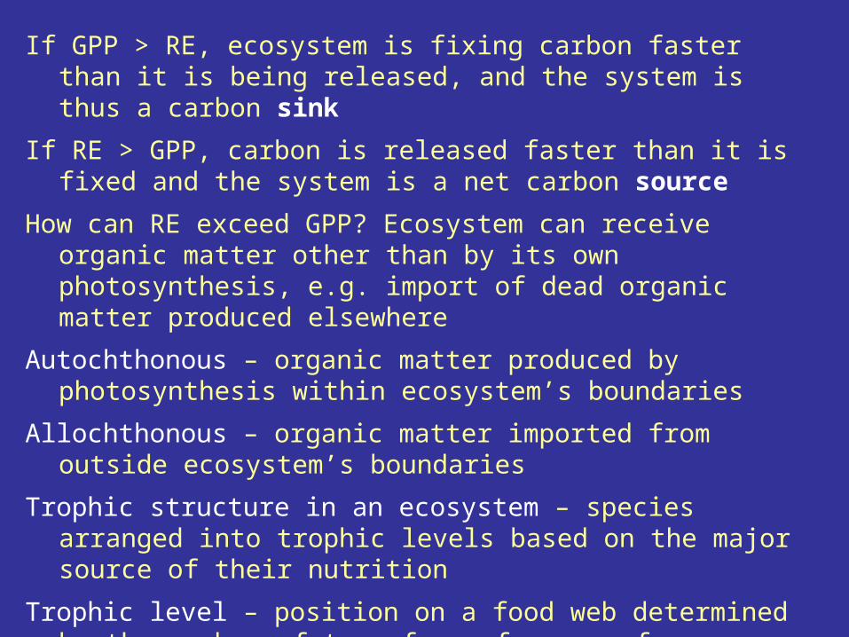
If GPP > RE, ecosystem is fixing carbon faster than it is being released, and the system is thus a carbon sink

If RE > GPP, carbon is released faster than it is fixed and the system is a net carbon source

How can RE exceed GPP? Ecosystem can receive organic matter other than by its own photosynthesis, e.g. import of dead organic matter produced elsewhere

Autochthonous – organic matter produced by photosynthesis within ecosystem’s boundaries

Allochthonous – organic matter imported from outside ecosystem’s boundaries

Trophic structure in an ecosystem – species arranged into trophic levels based on the major source of their nutrition

Trophic level – position on a food web determined by the number of transfers of energy from primary producers to that level

Trophic Levels

Fourth trophic level (large carnivores)

Third trophic level (carnivores)

Primary consumers (herbivores)

Primary producers (plants)

Inorganic energy (solar energy) plus water, CO2, etc.

Global Primary Production

NPP of Earth about 105 petagrams of carbon per year (1 petagram (Pg) = 1015 g)

Terrestrial ecosystems 56.4 Pg C yr-1

Aquatic ecosystems 48.3 Pg C yr-1

Although oceans 72% of Earth’s surface, account for 46% of Earth’s total NPP

On land, tropical rainforest and savannas account for 60% of terrestrial NPP and 32% of Earth’s total NPP

Forest biomes show trend of increasing GPP with decreasing latitude

Grassland biomes show similar trend in above-ground NPP (ANPP) and below-ground NPP (BNPP)

In aquatic systems, similar latitudinal gradient in GPP of lakes.

Not in oceans where GPP more limited by nutrients and is high where there are upwellings of nutrient-rich waters, even at high latitudes and hence low temperatures.

Terrestrial trends suggest that radiation (a resource) and hence temperature (a condition) may limit productivity. But other factors frequently constrain productivity, even within narrow limits.

Mainly determined by temp and moisture at biome scale.

Terrestrial biomes in World Vegetation Biomes (Lecture 6) differ in their NPP

BiomeNPP (g m-2 yr-1)

Mean RangeArea

(106 km2)World NPP

(109 dry ton yr-1)

Tropical forest 2000 1000-3500 25 50

Savanna 900 200-2000 15 14

Desert 40 0-250 42 2

Temperate forest 1250 600-2500 12 15

Temperate woodland & shrubland

700 250-1200 9 6

Temperate grassland 600 200-1500 9 5

Boreal forest 800 400-2000 12 10

Tundra 140 10-400 8 1

Cultivated land 650 100-3500 14 9

Patterns of Terrestrial Primary Production

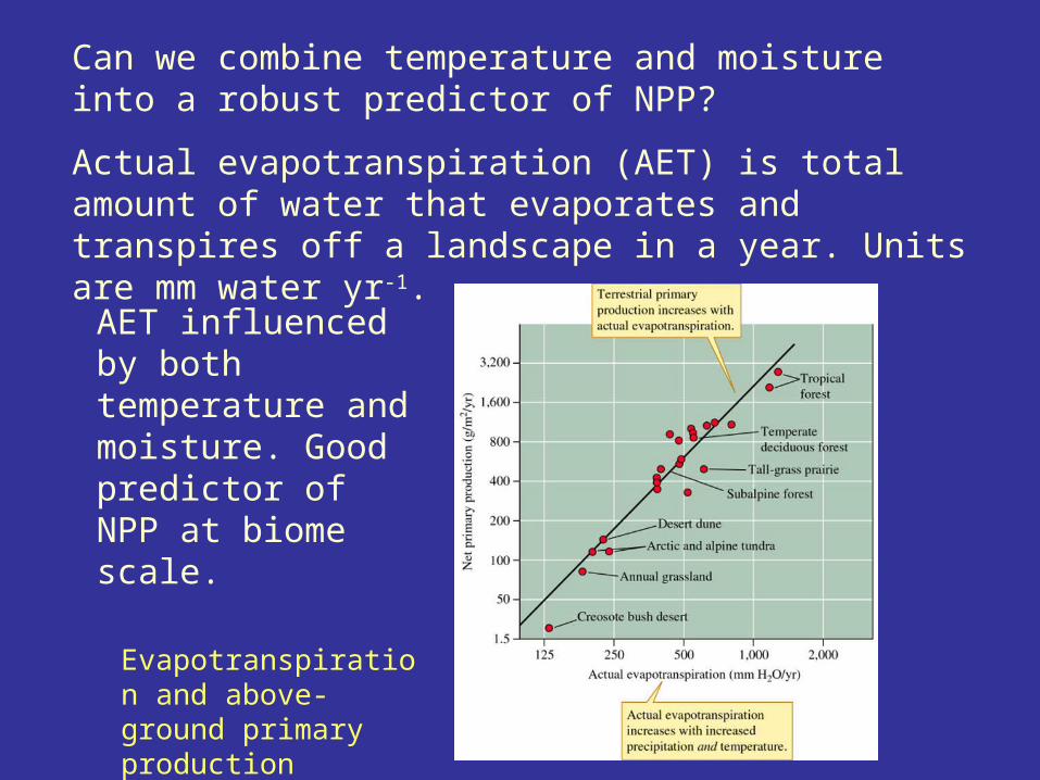
Can we combine temperature and moisture into a robust predictor of NPP?

Actual evapotranspiration (AET) is total amount of water that evaporates and transpires off a landscape in a year. Units are mm water yr-1.

AET influenced by both temperature and moisture. Good predictor of NPP at biome scale.

Evapotranspiration and above-ground primary production

Important to note that AET has not been measured. It is estimated from latitude, mean monthly temperature, and mean monthly precipitation.

Also AET is bound to be greater the more plant leaf area there is, as large leaves increase chances of water being transpired or evaporated rather than reaching the soil.

In addition, NPP will be greatest in communities with large leaf areas.

NPP and AET are not strictly independent variables – both are functions of leaf area, in particular leaf area index – number of leaves a typical vertical ray of sun-light passes through before hitting soil (range from <1 to >9 globally).

Major influence of annual precipitation

What determines variation in primary production within similar ecosystems?

Temperate grasslands in central US

Well known to farmers that productivity can be increased by adding fertilizers to soil.

Liebig (1840) nutrients limited plant growth.

At fine scale, soil fertility can influence productivity.

Addition of N, P, and K to Alaskan arctic tundra

2-4 years, NPP increased by 23-300% at all sites

Adding fertilizer to arctic tundra

Effect of fertilizers on wet and dry alpine tundra environments

Colorado alpine tundra

Added P, N, or N + P to dry and wet meadow tundra

Large effects (relative to control) in dry meadows

N may be limiting in dry meadow

N + P may be limiting in wet meadow.

How important is nitrogen-limitation on terrestrial net primary production?

Le Bauer and Treseder 2008 Ecology 89: 371-379

126 Nitrogen addition terrestrial experiments world-wide. Looked at effects on NPP ('meta-analysis')

Used response ratio

R = ANPPN/ANPPCTRL

where ANPP = above-ground NPP, N = nitrogen addition, and CTRL = control

R = 1.29 for all experiments

R

Temperate forests 1.19

Tropical forests 1.60*

Temperate grasslands 1.53

Tropical grasslands 1.26

Wetlands 1.16

Tundra 1.35

Deserts 1.11 not significant

*Tropical forests

Young volcanic soils (Hawaii)

2.13

'Old' soils 1.20 (very similar to temperate forests)

Are there any relationships between R (measure of N limitation) and latitude or climate?

Suggests that global N and C cycles interact strongly and that geography can influence ecosystem response to N within certain biome types (e.g. tundra, wetlands, grasslands).

Latitude Mean annual T

Mean annual pptn

All - - -Wetlands + - +Forests (all) + + +Forests (old soils only) - - -Grasslands + - -Tundra - + -

(+ significant at p < 0.05)

Seasonal and annual trends in terrestrial primary production (GPP)

Can vary in an ecosystem by a factor of 2, presumably due to annual fluctuations in temperature and rainfall

Within a year, GPP depends on seasonal variations in conditions, especially temperature and the length of the growing season

Period of high GPP longer in temperate forests than boreal forests

Summary of factors limiting primary production in terrestrial ecosystems

Resources: Solar radiation, CO2, Water, Soil nutrients

Condition: Temperature

Remember that

1. terrestrial systems use radiation inefficiently (self-shading)

2. photosynthetically active radiation may be limiting in some systems (e.g. C4 plants)

3. shortage of water is often a critical limiting factor

4. temperature and precipitation interact (‘energy-water’ model)

5. soil texture can influence productivity (dry vs. mesic)

6. length of growing season can be very important (tropics vs. boreal)

7. nutrient availability can also be limiting (N, P)

See Begon et al. (2006) pp. 505-511 for further details

72% world is covered by water, but only 46% of world's NPP is from aquatic systems.

TypeNPP (g m-2 yr-1)

Mean RangeArea

(106 km2)World NPP

(109 dry ton yr-1)

Swamps 2000 800-3500 2 4

Algal beds & coral reefs

1800 500-2000 2 4

Continental shelf 360 200-1000 27 10

Lakes & streams 250 100-1500 2 1

Oceans 125 2-400 332 42

Patterns of Aquatic Primary Production

Why lower NPP in aquatic systems?

Cannot be a shortage of water!

Some systems have high NPP (algal beds, swamps, coral reefs); ocean has low NPP (less than tundra!)

Why is the sea blue?

Physicist's answer – blue light with its short wavelength is less likely to be absorbed than red or green light. Light reflected back to our eyes is most likely to be blue.

Biologist's answer – it is blue because it is not green with plants!

So why are terrestrial systems mainly green and aquatic systems mainly blue?

Most aquatic systems are starved of nutrients.

What determines algal biomass?

Phosphorus concentration and algal biomass in lakes

What is the relation between algal biomass and rate of primary production?

Test ideas on aquatic productivity by whole-lake ecosystem manipulations.

Experimental Lakes Area, Ontario, Canada.

Lake 226 divided into sub-basins

C added to one basin

C, N, and P to other basin

1973-1980.

Measured phytoplankton biomass before, during, and after fertilization and in control lake.

Effect of nutrient additions

Clear that nutrient availability, especially phosphorus and nitrogen, controls rate of primary production in freshwater ecosystems.

What about marine ecosystems?

Much more difficult to study!

Main depth zones in the ocean – continental shelf, continental slope, abyssal plain

Main vertical life zones in the ocean. Almost all life depends on the phytoplankton growth in the epipelagic zone (0 - 150 m depth)

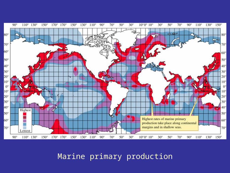
Marine primary production

Phytoplankton concentration in the Atlantic as shown in a satellite image. Note concentrations in northern half.

Highest production along continental shelves and in areas of upwelling.

Nutrients renewed by run-off from land and sediment redistribution.

Up-welling brings nutrient-rich water to surface.

These areas are not a clear blue but a murky green due to the high phytoplankton density. Start the aquatic food web. Great fishing areas of the world.

Main ocean has low nutrient availability and low rate of primary production.

Iron is limiting nutrient in about 30% of open ocean. Very insoluble in sea-water. Main input is wind-blown particulate material.

Nutrient renewal in open ocean is by vertical mixing. Such mixing is often blocked in open tropical oceans by a permanent thermocline.

Open tropical oceans thus have low nutrient concentrations and hence lowest rates of primary productivity (< arctic tundra!).

Some marine primary producers in phytoplankton – epipelagic zone

Coccolithophorid (Coccolithus pelagicus)

Diatom

Dinoflagellate

Zooplankton – epipelagic zone

Jellyfish (Pentachogon sp.)

Krill (Euphausia superba)Arrow worms (Chaetognatha)

Copepod

Squid (Chiroteuthis)

Mesopelagic animals

Deep sea jellyfish (Atolla sp.)

Shrimp (Systellaspis debilis)

Deep red shrimp (Acanthephyra sp.)

Mesopelagic and Bathypelagic animals

Hatchet fish (Argyropelecus aculeatus)

Lantern fish (Myctophum punctatum)

Deep-sea squid (Watsenia scintillans)

Is there any experimental evidence for nutrient limitation in marine systems?

Difficult to do an Experimental Lake Area-type experiment with an ocean!

Edna Graneli (1990) Baltic Sea.

Collected filtered sea-water from 5 sites

looked at algal growth in control

with P added

and with N added.

Nitrate control of primary production

In contrast to freshwater systems, N limitation appears to be most important in some coastal and marine systems.

Himmelfjärden, Sweden – brackish inlet of Baltic Sea with area of 195 km2

N limitation can shift to P limitation by altering N:P ratios.

Adding P reinforces N limitation

Decreasing P and adding N leads to P limitation.

Nature is never simple!

Global survey of estuaries and coastal marine phytoplankton in relation to nitrogen and phosphorus – Val Smith (2006) L & O 51: 377-384

Chlorophyll a and annual mean total N concentrations in coastal marine systems

log10 Chl a = -3.71 + 4.26 log10TN – 0.88 (log10 TN)2

r2 = 0.84

Total N and coastal systems

Chlorophyll a and annual mean total P concentrations in coastal marine systems

log10 Chl a = 0.39 + 0.71 log10 TP

r2 = 0.60

Total P and coastal systems

Which is more important - total N or total P – in coastal systems?Redfield ratio – particulate N:P in marine organisms = 16:1 by moles

Total N and total P in coastal systems

Data almost divided into 2 by Redfield ratio

log10 TN = 1.38 + 0.41 log10 TP

r2 = 0.55

Cumulative frequencies of TN:TP ratios

See 50% of sites show evidence for phosphorus limitation, with TN:TP ratio >16

Pristine marine environments (annual TP < 0.8 mol P l-1) tend to have TN:TP ratios > Redfield ratio of 16 and thus are likely to be consistently P limited

Heavily nutrient-enriched environments (annual TP > 8 mol P l-1) have TN:TP < Redfield ratio and thus are likely to be consistently N limited

Both N-limited and P-limited marine sites

P-limited sites: log Chl a = 0.99 log TP + 0.11 r2 = 0.74

N-limited sites: log Chl a = 1.48 log TP + 0.61r2 = 0.69

Comparisons between lakes □ and coastal sites

A: All sites

B: TN:TP < 20, only N limited sites

C: TN:TP > 20 sites, only P limited sites

Similarity in physiological response of freshwater and marine phytoplankton to nutrients probably a result of the shared evolutionary histories of freshwater and marine phytoplankton.

Nature is both complex (total N, total P, and N:P ratios) and simple (freshwater and marine phytoplankton have shared histories)!

What else can determine algal biomass?

Phosphorus concentration and algal biomass in lakes

Scatter of points around relationship between P concentrations and algal biomass.

Residual variation in algal biomass not explained by P concentrations.

What other factors can influence algal biomass?

Influence of physical and chemical abiotic factors – BOTTOM-UP CONTROLS

Influence of consumers – TOP-DOWN CONTROLS

Influences of evapotranspiration, precipitation, or nutrients on productivity are all bottom-up controls.

What about top-down controls?

Role of Consumers on Rates of Primary Production

Trophic-Cascade Hypothesis

A change in one of the trophic levels will have a cascading effect on the rest of the food web.

Similar to the keystone species hypothesis in community ecology except that the trophic-cascade hypothesis is concerned with ecosystem processes such as productivity rather than species diversity.

Important to distinguish between species cascades and ecosystem trophic cascades. Trophic-cascade is now an ambiguous concept.

Trophic-cascade hypothesis 1. Large fish feed on smaller

fish and invertebrates

2. Large fish therefore influence zooplankton and large zooplankton (eaten by planktivorous fish) dominate the zooplankton

3. This reduces phyto-plankton biomass and rate of primary production

Trophic cascade consistent with negative correlation between zooplankton body size and primary production

Predicted effect of piscivores

Experimental manipulations of fish in two small lakes plus a third control lake.

Lake with large-mouth bass (piscivorous)

Lake with no bass but abundant minnows (planktivorous)

Removed 90% of large-mouth bass and put them in the other lake

Removed 90% of minnows and put them in the other lake

Experimental manipulation of lakes and their responses

As predicted, reducing the planktivorous fish led to reduced primary production, as large zooplankton increased.

Adding planktivorous minnow fish led to increased primary production. By adding minnows, food for remaining bass, 50-fold increase in bass population that preyed on zooplankton, and phytoplankton increased.

Support for top-down controls in lakes.

What about marine systems?

Are long-term sustainable fish catches from the continental margin in marine ecosystems controlled by

(1) primary production rates (bottom-up controls)

or

(2) predator-prey interactions at higher trophic levels (top-down controls)?

Satellite derived estimates of chlorophyll-a concentrations to test hypothesis that fish production along the western North American continental shelf is mainly controlled by phytoplankton production (bottom-up controls)

Chlorophyll-a – a proxy measure for phytoplankton concentrations

Ware & Thompson 2005 Science 308: 1280-1284

Looked at two spatial scales (67,157 & 18,830 km2)

High correlation (r2 = 0.87) between fish yield and mean annual chlorophyll-a

concentrations at broad scale

Why are there spatial variations in the chlorophyll-a concentrations?

1. Negative correlation between chlorophyll-a and offshore winds and upwelling.

2. High correlation with year-round freshwater flux. Provides micronutrients and water column stability. Mainly in Washington – southern British Columbia regions, from Columbia and Fraser rivers.

At the finer, regional scale, correlation between fish yield and chlorophyll-a concentrations is high (r2 = 0.76)

Also high correlation (r2 = 0.85) between zooplankton productivity and chlorophyll-a concentrations

High correlation also between fish yield and zooplankton productivity (r2 = 0.79)

All consistent with bottom-up trophic control

Primary production by phytoplankton moved through the pelagic and benthic food-webs to the fish community.

Controlled by terrestrial nutrient supply and water column stability as a result of freshwater input from the major rivers.

Clear bottom-up trophic control and processes.

Is nature that simple?

Frank et al. 2005 Science 308: 1621-1623

Top-down trophic cascades (predator dominated) in a formerly cod-dominated ecosystem off Nova Scotia, Canada. 1963-2004

1. Collapse of benthic fish community (major predators) in mid 1980s. Mainly cod but also 10 other fish species.

2. Abundance of small pelagic fish and benthic macro-invertebrates increased markedly after benthic fish collapse. Correlations between benthic fish biomass and pelagic fish or macro-invertebrates all negative (r = -0.61 to -0.76)

3. With the removal of the top predator (cod and other large benthic fish) conspicuous indirect effects.

(a) herbivorous zooplankton declined as benthic fish declined (r = 0.45) and small fish increased (r = 0.52). Change from large to small size, resulting from size-selective predation on zooplankton by pelagic fish that increased with decline of cod.

(b) phytoplankton increased as benthic fish declined (r = -0.72) as less herbivorous zooplankton.

Cod decline

in 1980s

More small predators

Less large predators

Increase of small pelagic

fish & benthic macro-

invertebrates

Less herbivory

More nutrient

utilisation

Decline of herbivorous zooplankton

& size change;

large - small

Increase of phytoplankton as less

herbivorous zooplankton

Decrease of nitrate, major limiting factor,

due to increased

phytoplankton

Top-down cascading effects before and after the collapse of cod and other large predators on the Nova Scotia shelf in mid 1980s

Scheffer et al. 2005

Trophic cascade here involves four trophic levels and nutrients. Driven by changes in the abundance of top predator (primarily cod).

Top-down control with indirect effects and multiple links.

Change from benthic fish commercial fishery >100 x 103 metric tons (kt) to pelagic fish – macroinvertebrate system with poor benthic fishery of <50 kt. Attempts to reverse the trend have failed so far.

Shows strong non-linearities in community behaviour and regime shifts induced by over-exploitation.

Nature is never simple!

Are there any top-down trophic cascades on land or are 'top-down' trophic cascades all wet?

Grazing by Large Mammals

Serengeti-Mara grasslands (25 000 km2) on Tanzania-Kenya border

One of the last ecosystems where huge numbers of large mammals still roam

Photo: John Grimshaw

Grazers consume 66% of annual primary production

Complex interaction of abiotic and biotic factors

Soil fertility and rainfall stimulate plant growth, hence grazing mammals

Grazing mammals also affect water balance, soil fertility, and plant production

Compensatory plant growth in area grazed by wildebeest. Grazing increases the growth rate of many grass species. Possible mechanisms include lower rates of respiration due to lower plant biomass, reduced shelf-shading, and improved water balance due to reduced leaf area.

Growth response of grasses grazed by wildebeest

Compensatory growth highest at intermediate grazing intensities

"African ecosystems cannot be understood without close consideration of the large mammals. These animals interact with their habitats in complex and powerful patterns, influencing ecosystems for long periods."

Serengeti system is a terrestrial trophic cascade of top-down controls, with wildebeest influencing primary production.

Are trophic cascades widespread? What factors determine the occurrence of trophic cascades?

Factors and processes that may influence the occurrence of trophic cascades (based on 41 studies)

Factor Net effect

Factor Net effect

Self-regulation Landscape features Cannibalism - Disturbance patterns + or - Interference competition - Spatial variation + or - Territoriality - Refugia - Inter-guild predation -Regulation across trophic levels

Resource availability and quality

Omnivory + or - Low resource quality - Intra-guild predation + or - High resource quality + Predation-mediated

coexistence- Resource dominated by

few species+

Behavioural responses + or - Temporal heterogeneity + or - Positive interactions + or - Rapid nutrient cycling + Consumer age-structure + or - Food-web complexity -

Not all ecosystems will show trophic cascades. Effects of different factors are

negative (8)

positive (3)

either negative or positive (8) depending on other factors

Trophic cascades appear to be common in freshwater and marine systems but rare in terrestrial systems

Why are aquatic and terrestrial systems different?

Aquatic Terrestrial

Discrete, homogeneous habitats

Fuzzy, heterogeneous habitats

Prey populations dynamics rapid relative to predator dynamics (e.g. rapid algal turnover)

Variable prey population dynamics

Common prey are uniformly edible

Common prey not uniformly edible

Systems simple and trophically stratified

Systems complex and reticulate and species interactions weak and diffuse

But terrestrial agricultural systems may be the exception that proves the rule. Such systems tend to have the features of aquatic systems.

Suggests that more diverse systems are tied together by multiple trophic influences among species. Less likelihood of trophic cascades in diverse systems, including many natural or semi-natural terrestrial systems.

Nature is never simple!

What is the Relationship Between Productivity and Standing-Crop

Biomass?

Can think of standing crop as the biomass sustained by the productivity (capital resource sustained by earnings)

Can think of productivity as a function of the standing crop that produces it (interest rate on the capital)

Total biomass – land 800 Pgoceans 2 Pgfreshwater <0.1 Pg

Allowing for area – land 0.2 – 200 kg m-2

oceans <0.001 – 6 kg m-2

freshwater <0.1 kg m-2

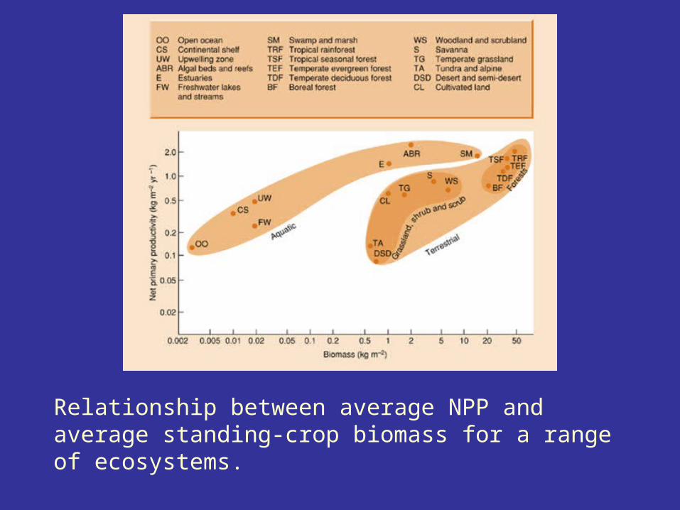
Relationship between average NPP and average standing-crop biomass for a range of ecosystems.

1. Higher NPP produced by a smaller biomass (B) in non-forest systems, and in aquatic systems

2. NPP:Biomass (kg dry matter produced per year per kg of standing crop) is

0.042 forests0.29 other terrestrial systems17 aquatic systems

3. Reason is that much of forest biomass is dead (and has been for some time) and much of supporting tissue (wood) is not photosynthetic

4. In grasslands, higher fraction of biomass is alive and is photosynthetic, but 50% of biomass may be roots

5. In aquatic systems, especially where NPP is dominated by phytoplankton, there is no support tissue, no roots, no accumulation of dead cells, and the photosynthetic output per kg of biomass is thus very high

6. High NPP:B ratios in aquatic systems also due to rapid turnover of biomass (aquatic systems 0.02-0.06 years turnover time of biomass, terrestrial systems 1-20 years)

In succession, NPP:B tends to decrease

1. Early successional pioneers (rapidly growing herbs) have little support tissue so NPP:B is high

2. Late successional plants (shrubs and trees) have much support tissue and NPP:B is low

3. Within trees, common pattern is for above-ground NPP to peak early in succession and then gradually decline by as much as 76%, with a mean reduction of 34% later in the succession

Shift from primarily photosynthetic to respiring tissues, along with nutrient limitation (N, then P)

Trees of different successional stages show different patterns of NPP with stand age

Early successional Pinus albicaulis (whitebark pine) –peak NPP about 250 yrs

Late successional Abies lasiocarpa (subalpine fir) – peak NPP after 400 yrs

200% more biomass in fir foliage than in pine, maintains high photosynthesis:respiration ratio to greater age than pine

Trophic Levels

Idea of energy transfer from one level to another –

primary producers

primary consumers

carnivores

etc.

Chapman & Reiss

In natural ecosystems, usually only 2-5 trophic levels.

What limits the number of trophic levels?

Raymond E. Lindeman, University of Minnesota. Died aged 27 in 1942

Cedar Bog Lake.

Proposed concept of trophic dynamics – transfer of energy from one part of an ecosystem to another.

Trophic levels - primary producers

primary consumers

secondary consumers

etc.

Each level feeds on the one immediately below it.

Energy enters the ecosystem by photosynthesis by primary producers, converting solar energy into biomass.

As energy is transferred from one trophic level to another, energy is lost due to limited assimilation, respiration by consumers, and heat production.

Forms pyramid-shaped distribution of energy between trophic-levels. 'Eltonian pyramids' named after Charles Elton, the great Oxford animal ecologist.

Annual production by trophic level in two lakes

Ecosystems thus consist of

1. Autotrophs - photoautotrophs or primary producers

- chemoautotrophs fixing atmospheric N

2. Decomposers

3. Herbivores and carnivores

4. Omnivores

5. Organic sink

6. Atmosphere, minerals, and water

7. Solar energy

Amount of dead organic matter in biomes

Major organic sinks in northern areas

Tropical forest 2 tons ha-1

Temperate forest 15-30 tons ha-1

Boreal forest 30-45 tons ha-1

Tundra 85 tons ha-1

Energy Flow in a Temperate Forest

Hubbard Brook Experimental Forest, Eastern USA

Quantified energy flow as kilocalories (k cal) per square metre per year

Gene Likens Herbert Borman

Energy budget for a temperate deciduous forest (%)

Biomass k cal m-2

Dead organic matter 122,442(88,120 soil)(34,322 plant litter)

Total living-plant biomass 71,420(59,696 above ground)(11,724 below-ground)

Energy Budget

Solar energy 15% reflected, 41% converted into heat, 42% absorbed in evapotranspiration

Only 2.2% fixed by plants as gross primary production

Plant respiration 1.2%

NPP 1.0%

Net primary production ca. 4800 k cal m-2

Plant growth 1199 k cal m-2

Herbivores 41 k cal m-2

Litter fall 3037 k cal m-2

Detritus, root exudates, etc. 437 k cal m-2

Net primary production 1%

96% of this available to consumers is lost by consumer respiration.

Little energy left for a third trophic level.

It is the losses with each transfer of energy in a food chain that limits the number of trophic levels.

As these losses between levels accumulate, insufficient energy to support viable populations at a higher trophic level.

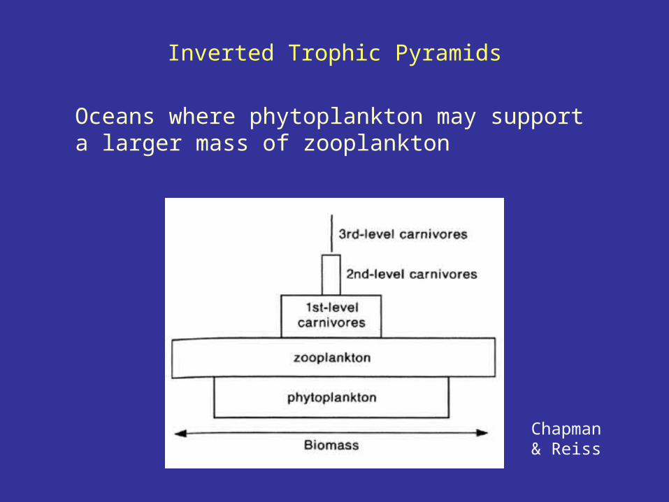
Inverted Trophic Pyramids

Oceans where phytoplankton may support a larger mass of zooplankton

Chapman & Reiss

Energy Flow Through Different Ecosystems

Three transfer efficiencies needed for quantitative comparison between systems

1. Consumption Efficiency (CE)

CE = In / Pn-1 x 100

Percentage of total productivity available at one trophic level (Pn-1) that is consumed by a trophic level one up (In)

5% in forests

25% in grasslands

50% in phytoplankton-dominated systems

2. Assimilation Efficiency (AE)

AE = An / In x 100

Percentages of food energy taken into guts of consumers at a trophic level (In) that is assimilated across the gut wall (An) and becomes available for growth, etc.

20-50% for herbivores

80% for carnivores

60-70% for seeds and fruits

50% for leaves

15% for wood

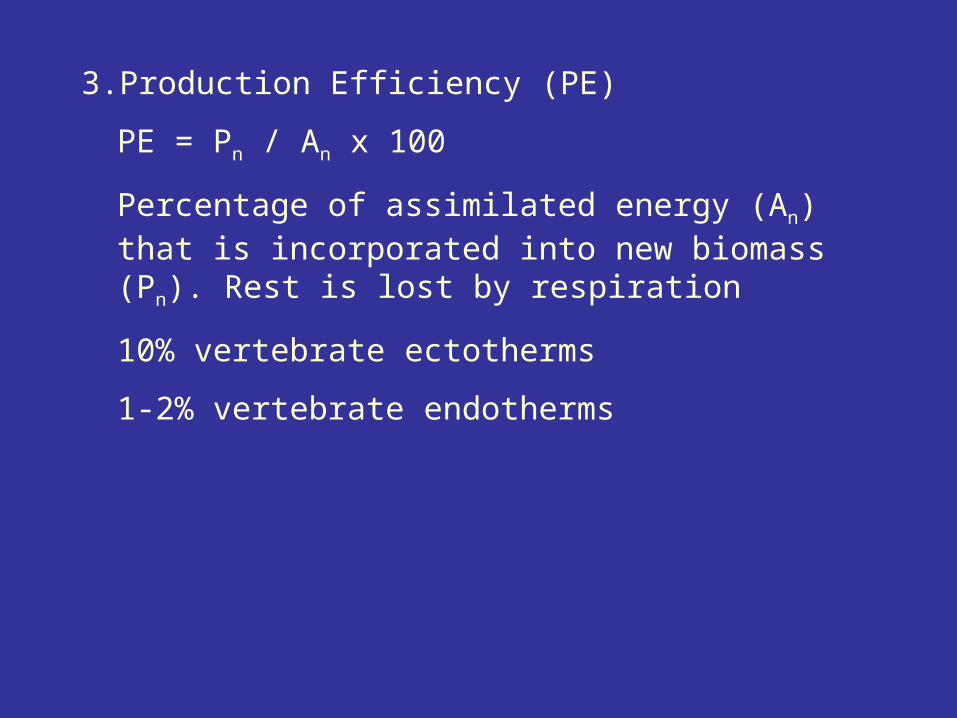
3. Production Efficiency (PE)

PE = Pn / An x 100

Percentage of assimilated energy (An) that is incorporated into new biomass (Pn). Rest is lost by respiration

10% vertebrate ectotherms

1-2% vertebrate endotherms

Overall trophic level transfer efficiency from one level to next is CE x AE x PE

Great variation in transfer efficiency

mean = 10.13%

SE = 0.49

No complete NPP, CE, AE, and PE data for any systems

Some general patterns for forests, grasslands, plankton-dominated systems, and freshwater streams

1. Decomposer system responsible for main ecosystem respiration (RE, mainly RH)

2. Grazers most important in plankton-system, least important in terrestrial and stream systems

3. Deep-ocean benthic system most like stream system, with low NPP, high dead organic carbon sinking from the euphotic zone above

DOM = dead organic matter; GS = grazer system

NPP for 9 systems (a) and estimates of how much NPP is consumed by herbivores (b), how much becomes detritus (c), how much persists as detritus (d), and how much is exported (e). See differences in herbivory, detritus production, long-lasting detritus production, and export.

Do Trophic Levels Exist?

1. How to decide to which level a particular species belongs?

2. Dead organisms, urine, and faeces are usually ignored but may represent a large amount of biomass.

3. Symbiotic bacteria in ruminant guts – are they herbivores or saprotrophs?

Can we use stable isotopes to identify energy sources?

Ribbed mussel Geukinsia demissa living in coastal salt-marshes on eastern coast of USA.

Primarily eats fine detritus as filter-feeder.

Detritus consists of:

1. Upland plant material brought in by rivers

2. Spartina salt-marsh grass

3. Phytoplankton

Using stable-isotope analysis of 13C, 15N, and 34S, could establish the isotope signature of potential food sources for the mussel.

Isotopic content of food sources for the ribbed mussel, Geukinisia demissa, in a New England salt-marsh

Upland C3 plants most depleted in 13C

Spartina (a C4 plant) least depleted in 13C

Plankton has highest concentrations of 34S

Variation in isotopic composition of ribbed mussels by distance inland

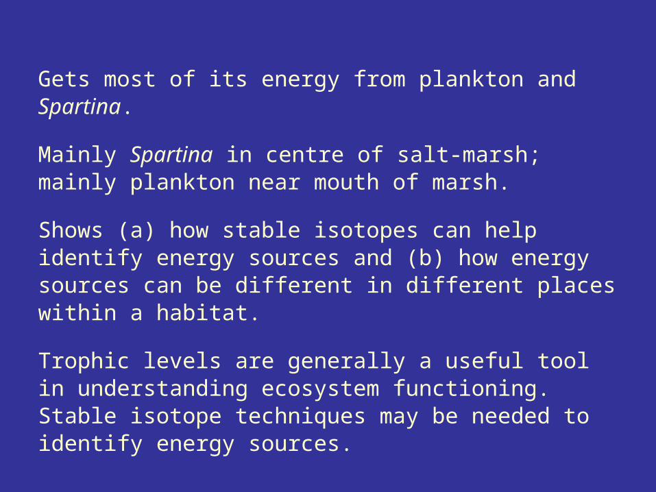
Gets most of its energy from plankton and Spartina.

Mainly Spartina in centre of salt-marsh; mainly plankton near mouth of marsh.

Shows (a) how stable isotopes can help identify energy sources and (b) how energy sources can be different in different places within a habitat.

Trophic levels are generally a useful tool in understanding ecosystem functioning. Stable isotope techniques may be needed to identify energy sources.

Why is the World Green?

Current estimates are that for every one plant species, there are at least five species of animal herbivore.

Why have grazing animals not consumed all the vegetation and reduced the Earth’s land to dust?

Hairston et al. (1960) hypothesise that herbivore numbers are controlled by predation by carnivores and by keeping herbivores in check, carnivores keep the world green and allow plant primary production to continue.

Difficult to test.

Terborough et al. 2006 J. Ecology 94: 253-263

Lago Guri, Venezuela formed by flooding of a broad valley for hydroelectric development

Lake is 4300 km2 and contains many islands of different sizes

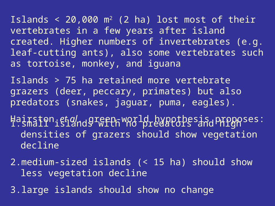
Islands < 20,000 m2 (2 ha) lost most of their vertebrates in a few years after island created. Higher numbers of invertebrates (e.g. leaf-cutting ants), also some vertebrates such as tortoise, monkey, and iguana

Islands > 75 ha retained more vertebrate grazers (deer, peccary, primates) but also predators (snakes, jaguar, puma, eagles).

Hairston et al. green-world hypothesis proposes:

1. small islands with no predators and high densities of grazers should show vegetation decline

2. medium-sized islands (< 15 ha) should show less vegetation decline

3. large islands should show no change

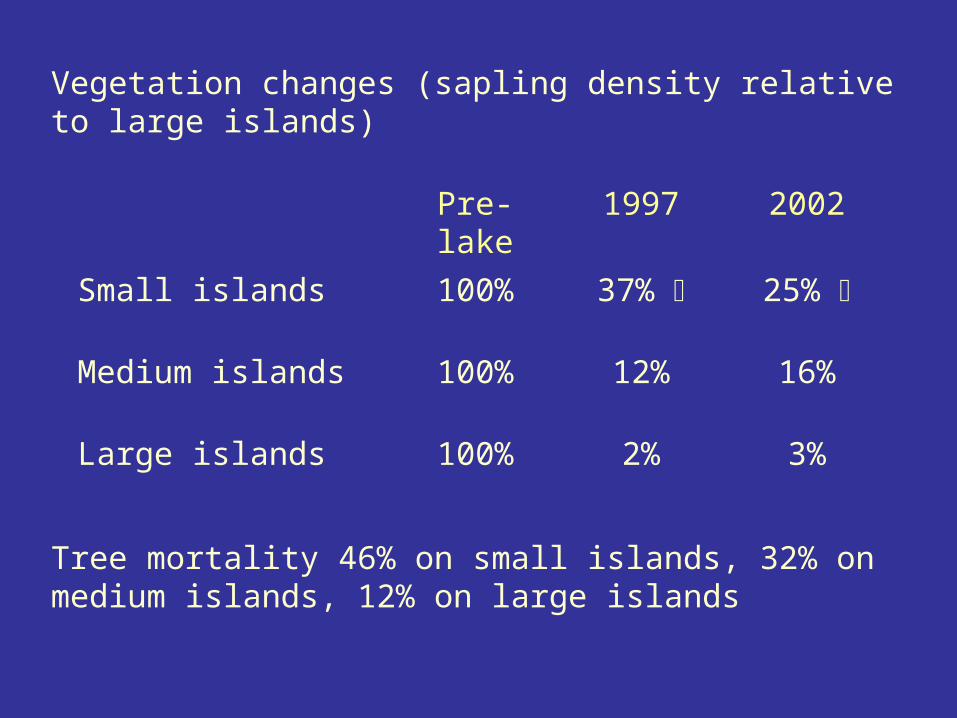
Vegetation changes (sapling density relative to large islands)

Pre-lake 1997 2002

Small islands 100% 37% 25%

Medium islands 100% 12% 16%

Large islands 100% 2% 3%

Tree mortality 46% on small islands, 32% on medium islands, 12% on large islands

Loss of predators on grazers and leaf-cutting ants on small islands resulted in a trophic cascade that destabilised food web.

Difficult to show in terrestrial systems (cf. Serengeti example above). Loss of wolf predators has resulted in increased grazers and overgrazing.

Will overgrazing on small islands in Lake Guri result in the total destruction of vegetation on these islands? Would this lead to an extinction of grazing herbivores? Would there then be re-invasion by different plant species and associated herbivores?

Importance of long-term ecological observations and regular monitoring to understand ecological processes.

Interactions Across EcosystemsA Complex Ecosystem with Marine-Terrestrial Links

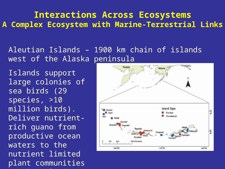
Aleutian Islands – 1900 km chain of islands west of the Alaska peninsula

Islands support large colonies of sea birds (29 species, >10 million birds). Deliver nutrient-rich guano from productive ocean waters to the nutrient limited plant communities on the islands.

Following collapse of the fur-hunting trade in late 19th and early 20th century, foxes were introduced to some but not all the islands as an extra source of fur.

Introduced foxes severely reduced the sea bird colonies on the islands where they were introduced.

Some islands remained free of foxes.

Large-scale natural experiment on the effects of top predators on sea bird numbers and hence on soil and plant nutrients, plant abundance, composition, and productivity, and nutrient flow.

Croll et al. 2005 Science 307: 1959-1961.

9 islands with foxes 9 islands without foxes

Sea bird density much greater (x2) on fox-free islands

Soil phosphorus x3 on fox-free islands

Grass biomass x3 on fox-free islands

Shrub biomass x10 LESS on fox-free islands

Nitrogen content on plants greater on fox-free islands

Vegetation on fox-free islands dominated by grasses

Vegetation on islands with foxes had more shrubs

Examined δ15N isotope values in soils, plants, and herbivores. Greater in soils on fox-free islands. Indicates that nutrients on fox-free islands are enriched by marine supply coming from sea-bird guano.

Introduction of foxes onto some islands has transformed islands from grasslands to shrub-tundra. Fox predation has reduced sea bird populations, thereby reducing nutrient transport from sea to land.

Trophic cascades are a series of strictly top-down interactions. Predators affect herbivore populations and alter the intensity of herbivory and hence the primary plant production at the base of the food web.

Aleutian Islands show that it is more complex because the predators have powerful indirect effects on the ecosystem by reducing the transport of nutrients between marine and terrestrial systems.

By preying on sea birds, foxes have reduced nutrient transport form ocean to land and have thus affected soil fertility and changed grasslands to dwarf-shrub dominated ecosystems.

Striking example of the complexity of nature and the interaction of different components in the ecosystem.

Nature is never simple!

Trophic Cascades Across Ecosystems

Knight et al. 2005 Nature 437: 880-883

Freshwater fish indirectly influence terrestrial plant reproduction through cascading trophic interactions across ecosystem boundaries.

Interaction web showing pathway by which fish facilitate plant reproduction

TOP-DOWN trophic cascades across ecosystems

8 ponds in northern Florida, 4 with fish, 4 without fish

Examined fish densities, larval and adult dragonfly densities and size, and plant pollinator visits by Diptera, Lepidoptera, and Hymenoptera insects.

Dragonflies were more abundant in and around ponds without fish than at ponds with fish. Predation of larvae by fish.

Large- and medium-sized dragonflies dominate by fish-free ponds; small-sized dragonflies at ponds with fish. Size-selection predation.

Pollinator visits much greater on Hypericum shrub by ponds with fish than by fish-free ponds. Ponds with fish mainly Hymenoptera (bees), ponds without fish mainly Diptera (flies).

Plant reproduction by fish-free ponds greatly limited by pollination compared to ponds with fish.

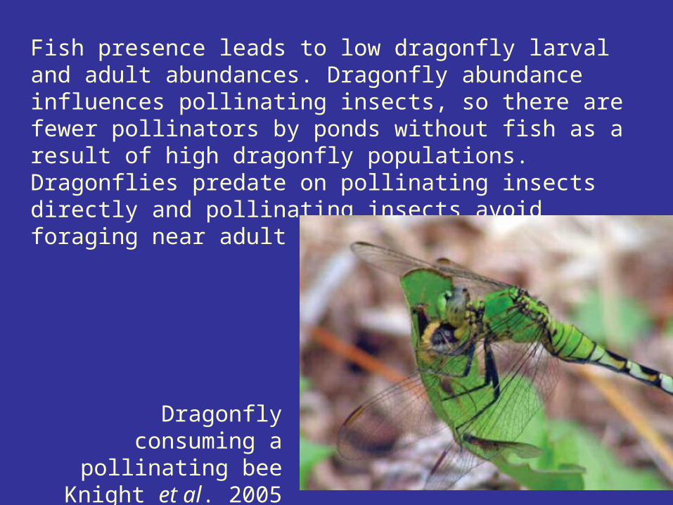
Fish presence leads to low dragonfly larval and adult abundances. Dragonfly abundance influences pollinating insects, so there are fewer pollinators by ponds without fish as a result of high dragonfly populations. Dragonflies predate on pollinating insects directly and pollinating insects avoid foraging near adult dragonflies.

Dragonfly consuming a pollinating bee

Knight et al. 2005

Clear example of interactions across ecosystem types. Many implications for conservation.

1. Deliberate fish introductions might have cascading effects on terrestrial systems, leading to increased reproductive success of insect-pollinated plants.

2. Could change competitive relationships between terrestrial plants, as insect-pollinated plants would be at an advantage.

3. Destruction of wetlands decrease dragonfly populations, with effects on terrestrial plants and their pollinators.

4. Decline in fish abundance (e.g. due to pollution) would affect dragonflies, and hence pollinating insects and plant reproduction.

Shows how predation in one system can affect another system and how local interactions can have community- and landscape-level effects.

Nature is never simple!

Conclusions and Summary1. An ecosystem is a biological community (or several

communities) plus all the abiotic factors influencing the community or communities.

2. Life on earth depends on primary production by plants.

3. Gross primary production (GPP) is the total amount of energy fixed by all the autotrophs in the ecosystem.

4. Net primary production (NPP) is the amount of energy left over after all autotrophs have respired and met their energy needs.

5. Ecosystems contain a small number of trophic levels and have a trophic structure.

6. GPP in terrestrial systems is about 2.7 x NPP, GPP in oceans is about 1.5 x NPP.

7. Tropical forest has the highest global NPP.

8. Terrestrial primary production is generally limited by temperature and moisture. Actual evapotranspiration (AET) is positively correlated with NPP in terrestrial systems. At finer scales within biomes, soil fertility can be important. NPP can vary from year to year.

9. Aquatic productivity is generally limited by nutrient availability.

10. Oceans have low NPP.

11. Phosphorus concentrations usually limit rates of primary production in freshwaters, whereas nitrogen concentrations usually limit rates in marine systems. Both systems can be limited either by N or P. Depends on N:P ratio.

12. Consumers can influence rates of primary production in aquatic and terrestrial systems.

13. Evidence for both bottom-up controls (abiotic) and top-down controls (biotic).

14. Trophic-cascade hypothesis proposes that a change in one trophic level may have a cascading effect on the rest of the trophic structure.

15. There is evidence for trophic-cascade hypothesis from both freshwater and terrestrial systems. Marine systems appear to be bottom-up or top-down systems. Trophic cascades are a result of many factors and interactions between factors.

16. There are some relationships between NPP:Biomass ratios within major systems (forests, other terrestrial systems, aquatic systems).

17. The number of trophic levels in an ecosystem is determined by the energy loss from one trophic level to the next level.

18. Trophic levels are a useful tool in understanding ecosystem functioning, but like guilds, plant life-forms, or plant functional-types, they are often abstractions.

19. Different ecosystems differ in their transfer efficiency between trophic levels.

20. Different ecosystems differ in the magnitude of herbivores, decomposers, and organic export.

21. Carnivores play an important role in influencing herbivore densities and hence grazing intensity and plant NPP.

22. Nature is never simple, only demanding and surprisingly complex!

EECRG Research Topics in this Lecture

Plant-animal interactions and their impact on growth in alpine environments

Primary productivity changes at tree-line in the Himalaya

www.eecrg.uib.no