3 lea valinsky , alexandra j. scupham1, gianluca della...
TRANSCRIPT

1
Oligonucleotide Fingerprinting of Ribosomal RNA Genes (OFRG) 1
2
LEA VALINSKY1, ALEXANDRA J. SCUPHAM1, GIANLUCA DELLA VEDOVA4, ZHENG 3
LIU2, ANDRES FIGUEROA2, KATECHAN JAMPACHAISRI3, BEI YIN1, ELIZABETH 4
BENT1, ROBERT MANCINI-JONES1, JAMES PRESS3, TAO JIANG2, and JAMES 5
BORNEMAN1 6
7
Departments of Plant Pathology1, Computer Science2, and Statistics3, University of California, Riverside, CA 92521 USA, Dipartimento di 8
Statistica4, Università degli Studi di Milano-Bicocca, via Bicocca degli Arcimboldi, 8, I-20126, Milano, Italy. 9
10
Introduction 11
12
Microorganisms are crucial components of ecosystems and human civilization. They play vital 13
roles in processes such as soil formation, nutrient cycling, detoxification of contaminated 14
environments, and the transformation of waste materials into useful commodities such as 15
compost [1, 16]. In the plant rhizosphere, they help decompose organic matter providing 16
essential nutrients required for plant growth [1, 8]. For biotechnology, microorganisms contain a 17
considerable resource of potentially useful compounds and enzymes, and provide vehicles for the 18
production of genetically engineered products [5, 7]. Despite these gains in basic knowledge and 19
biotechnology, the microbial contribution to ecosystem functioning and their potential for society 20
has yet to be fully realized, as thorough assessments of microbial diversity have been hindered 21
by technological limitations. 22
23

2
Oligonucleotide fingerprinting of ribosomal RNA genes (OFRG) is an array-based 1
method that enables extensive analysis of microbial community composition by sorting rRNA 2
gene clones into taxonomic clusters [17, 18]. Clone libraries are constructed using PCR primers 3
designed to selectively amplify ribosomal RNA genes from a specific taxonomic group. The 4
cloned rDNA fragments are arrayed on nylon membranes and then subjected to a series of 5
hybridization experiments, each using a single DNA oligonucleotide probe. For every 6
hybridization experiment, the signal intensities are transformed into three discrete values 0, 1, 7
and N, where 0 and 1 respectively specify negative and positive hybridization events and N 8
designates an uncertain assignment. This process creates a hybridization fingerprint for each 9
clone, which is a vector of values resulting from its hybridizations with all probes. The clones are 10
identified by clustering their hybridization fingerprints with those of known sequences and by 11
nucleotide sequence analyses of representative clones within a cluster. Alternative methods for 12
both transforming the hybridization data and clustering the hybridization fingerprints have also 13
been recently developed (see Tools for Data Analysis section). 14
15
Procedures 16
17
The OFRG process can be divided into six parts: (1) DNA extraction, (2) PCR of rRNA 18
genes, (3) Clone library construction, (4) Array construction, (5) Array hybridization, and 19
(6) Data analysis. 20
21
DNA extraction 22
23

3
Extract DNA from the sample of interest using an appropriate method. For soil, the Fast 1
DNA Spin Kit for Soil (Qbiogene, Carlsbad, CA, USA) or UltraClean Soil DNA Kit (Mo 2
Bio Laboratories, Carlsbad, CA, USA) work well. The inclusion of AlNH4(SO4)2 in the 3
extraction process may be useful to remove PCR inhibitors from the DNA [4]. Extract 4
DNA from replicate samples, pool an aliquot from each sample, and reduce the volume 5
of this pooled sample using a concentrator system such as the Savant Speed Vac 6
System. Purify the DNA by subjecting it to electrophoresis in an agarose gel, excising 7
the portion of the gel containing the larger fragments and isolating the DNA using a kit 8
such as the QIAquick Gel Extraction Kit (Qiagen, Valencia, CA, USA). PCR amplify 9
rRNA genes from this purified DNA as follows. 10
11
PCR amplification of rRNA genes 12
13
PCR optimization. Several factors need to be considered when optimizing PCR 14
conditions. (i) Template concentration may affect library composition [6]. (ii) Some DNA 15
samples contain substances that inhibit amplification. Gel isolation is an effective way to 16
purify DNA for PCR amplification. Diluting the template or adding BSA or other 17
components to the amplification reaction can also alleviate the inhibition [11, 14]. (iii) 18
The optimum number of PCR cycles is the fewest possible. We define this to be the 19
fewest number of cycles that produces a DNA band that is barely visible when 5 µl of an 20
amplification reaction is resolved on a 1% agarose gel and stained with ethidium 21
bromide. (iv) Zhou et al. present useful guidelines for reducing the number of chimeras 22
and heteroduplexes [13]. 23

4
1
PCR for library construction. Carry out 200 µl amplification reactions for each sample 2
using the optimized PCR conditions determined above. PCR reagents and cycling 3
parameters can vary. We typically perform 200 µl reactions that contain 50 mM Tris-HCl 4
(pH 8.3), 2.5 mM MgCl2, 500 µg/ml BSA, 250 µM of each dNTP, 400 nM each primer 5
(HPLC purified), and 10 U AmpliTaq DNA Polymerase (Applied Biosystems, Foster City, 6
CA, USA). The bacterial rRNA gene-selective primers are: 27fOFRG (forward), 7
AGRRTTTGATYHTGGYTCAG and 1492rOFRG (reverse), GBTACCTTGTTACGACTT, 8
which are modified versions of 27f and 1492r [12]. Given the high number of degenerate 9
positions in the 27fOFRG primer, amplification efficiency may be enhanced by 10
increasing its concentration to 4 µM. The fungal rDNA primers are: nu-SSU-0817-5’ 11
(forward), TTAGCATGGAATAATRRAATAGGA and nu-SSU-1536-3’ (reverse), 12
ATTGCAATGCYCTATCCCCA [3]. Cycling parameters for bacterial rRNA genes are: 13
94oC for 5 min; followed by x cycles at 94oC for 30 sec, 48oC for 30 sec, 72oC for 4 min; 14
followed by a 2 min incubation at 72oC. Cycling parameters for fungal rDNA are: 94oC 15
for 5 min; followed by x cycles at 94oC for 30 sec, 56oC for 30 sec, 72oC for 2 min; 16
followed by a 2 min incubation at 72oC. The number of cycles (x) is determined by 17
optimization experiments described in the previous section. (After these reactions have 18
been completed, an optional step can be performed to reduce the number of 19
heteroduplexes [15].) Use a concentrator system such as the Savant Speed Vac 20
System to reduce the volume of the amplification reactions to 5-10 µl. Resolve DNA on 21
a 1% agarose gel. Excise the bands containing the rRNA gene fragments and isolate 22
the DNA using a kit such as the Mini Elute Gel Extraction Kit (Qiagen). 23

5
1
rRNA gene clone library construction 2
3
Clone rDNA fragments using a T-vector system such as pGEM-T Vector System 4
(Promega, Madison, WI, USA) or other suitable vector following the instructions 5
provided by the manufacturer. Alternatively, preliminary experiments in our lab suggest 6
that the USER Friendly Cloning Kit (New England Biolabs, Beverly, MA) may be a 7
superior cloning system. It provides directional cloning and it appears to enhance 8
cloning efficiency. Note: if this system is used, additional nucleotides will need to be 9
added to the 5’ ends of the PCR primers (rDNA-selective) as described by the 10
manufacturer; in addition, new primers will need to be developed that specifically anneal 11
to the multiple cloning site of this vector for amplifying the rRNA genes for array printing. 12
13
Array construction 14
15
These instructions are for constructing arrays composed of 1536 rDNA clones. Note: 16
maintaining the orientation of the 384 well culture and PCR plates is very important. 17
Number the upper right corner of the plates (1-4). This helps keep the plates in a 18
uniform orientation throughout the procedure. 19
20
Colony selection and transfer. Transfer white colonies (those containing rRNA gene 21
inserts) into 384-well plates containing Luria-Bertani (LB) media (100 µg/ml ampicillin) 22
using toothpicks or another suitable transfer strategy. Each well should contain 30 µl of 23

6
medium except for the perimeter wells, which should contain 60 µl because the medium 1
in these wells evaporates more quickly. After inoculating a well, leave the toothpick 2
temporarily in the well. This directs the placement of the next inoculation. Do not leave 3
toothpicks in the wells for very long, because they absorb the medium. Toothpicks can 4
be reused after autoclaving. For two of the 384-well plates (plates 2 and 4 work best), 5
inoculate the column on the right side of the plate with positive and negative array 6
controls, which are clones that have defined nucleotide sequences. Note: for each 7
probe, there must be at least one control clone that will hybridize (positive control) and 8
one that does not hybridize (negative control). See the Data Analysis section for an 9
explanation of how these controls are used. 10
11
Clone library growth. Place the plates in an unsealed plastic bag with the open edge 12
folded under to prevent excessive drying. Grow the bacteria in this bag for 16-18 hours 13
at 37oC with shaking at 300 rpm. After this growth period, these bacteria are used for 14
the subsequent PCR step and are also stored for future use as described below. 15
16
PCR. PCR is performed by inoculating the reaction mix with the bacteria cultured in 17
384-well plates (as described above), which contain rRNA gene templates. PCR can be 18
performed using a thermocycler capable of holding 384-well plates or with water baths. 19
The water bath method has the advantage of allowing all PCR amplifications to be 20
performed simultaneously, which can reduce variation and therefore minimize error. 21
Note: the water bath method also requires that the 384-well plates be sealed using a 22
device such as the Combi Thermo-sealer (ABgene, Epsom, UK). 23

7
1
1. Clean a 384-pin, 0.5 µl slot pin replicator (VP 384S.5) (V&P Scientific, San 2
Diego, CA) with V&P Scientific Pin Cleaning Solution as described by the 3
manufacturer: add diluted cleaning solution (1 part cleaning solution, 4 parts 4
distilled water) to a pipette tip box lid (or other suitable container) until 1 cm deep. 5
Prepare three additional wash stations in pipette tip box lids: fill two with distilled 6
water and one with alcohol (95-100% EtOH, Isopropanol or Methanol) until 1 cm 7
deep. (i) Submerge replicator pins in cleaning solution. (ii) Blot on 8
chromatography paper (0.35 mm thick) or Lint-Free Blotting Paper (V&P 9
Scientific). (iii) Submerge replicator pins in distilled water. (iv) Blot on 10
chromatography paper (0.35 mm thick) or Lint-Free Blotting Paper. (v) Repeat 11
steps iii and iv using clean water. (vi) Submerge replicator pins in alcohol. (vii) 12
Dry the pins by using a hair drier or by flaming the alcohol. 13
2. Make reaction mix for four 384-well plates and store on ice. Combine 41 ml H2O, 14
6 ml 0.5 M Tris pH 8.3, 6 ml 25 mM MgCl2, 3 ml 10 µg/ml BSA, 3 ml dNTPs mix 15
containing 5mM each dNTP, 240 µl 100 µM primer T725, 16
GGCCCGACGTCGCATGCTC (HPLC purified), 240 µl 100 µM primer SP650, 17
TGGTCGACCTGCAGGCGGC (HPLC purified), and 3000 Units Taq DNA 18
Polymerase. Note: these primers anneal to the multiple cloning site of pGEM-T. If 19
another vector is used for cloning, different PCR primers will be needed. 20
3. Place four 384-well PCR plates on ice and add 35 µl reaction mix to each well. 21
To avoid bubbles at the bottom of the wells, which can lead to the displacement 22
of reaction mix when inoculated with the bacteria (Step 5), fill the wells by placing 23

8
the pipette tips at the bottom of the wells and then pull the pipette tips out of the 1
well while simultaneously dispensing the reaction mix. 2
4. If using the water bath method, turn on the Combi Thermo-sealer (ABgene, 3
Epsom, UK), which needs about 10 min to warm up. 4
5. Samples from the 384-well culture plates are transferred to the PCR reaction 5
plates using the 0.5 µl slot pin replicator. Inoculate the PCR plates with the 6
freshly grown bacteria described above. Pay attention to the plate numbers and 7
orientation. Inoculate 0.5 µl of each bacterial culture 2 to 4 times such that a total 8
of 1 to 2 µl is transferred to each well. Note: larger amounts (up to 10% of total 9
PCR volume) of bacteria may generate more PCR product, which typically 10
enhances the hybridization signal intensities and the overall performance of the 11
OFRG process. V&P Scientific will construct pin replicators that deliver a wide 12
range of volumes. It may be advantageous to use a 1 or 2 µl slot pin replicator 13
such that only one transfer is needed. If several inoculations are being performed 14
with a 0.5 µl replicator to transfer a total of 1-2 µl, dry the pins between 15
inoculations with alcohol and flaming to ensure accurate and consistent volume 16
transfers. 17
6. To prevent carry over from one 384-well plate to another, the replicator needs to 18
be cleaned between inoculating each different plate. Prepare three wash stations 19
in pipette tip box lids. The first station should contain 10% bleach, the second 20
distilled water, and the third alcohol (95-100% EtOH, Isopropanol or Methanol). 21
Blot the pins on chromatography paper (0.35 mm thick) or Lint-Free Blotting 22
Paper. Successively dip the pins in each wash station while blotting them on 23

9
chromatography paper (0.35 mm thick) or Lint-Free Blotting Paper between each 1
wash. Each successive station should contain slightly more solution to ensure 2
removal of the previous solution. After dipping the pins in alcohol, dry them using 3
a hair dryer or by flaming the alcohol. 4
7. If using the water bath method, seal the PCR plates using a Combi Thermo-5
sealer (ABgene, Epsom, UK) and Thermo-Seal foil (Marsh Bio Products, 6
Rochester, NY, USA) glossy side up. Press and hold the sealer on the plate for 7
exactly 3 sec, turn the plate 180o, press and hold the sealer on the plate for an 8
additional 1 sec. The plates will not seal properly if the top surface of the plate is 9
wet, which could occur for several reasons. First, care must be taken when filling 10
the wells with the PCR reaction mix. Second, if bubbles were introduced when 11
filling the wells, this mixture may overflow from the wells when the mix is 12
inoculated with the bacteria. If using a conventional thermocycler, use an 13
appropriate sealing material. 14
8. Perform thermocycling: 10 min at 94oC; 35 cycles of 1 min at 94oC then 2 min at 15
72oC; 5 min at 72oC. Store PCR products at 4oC. 16
17
Clone library storage. After the amplification reactions have been inoculated, the 18
bacteria are stored for future use. This can be done in three ways. (1) The original set of 19
culture plates can also be stored at -70 or -80oC after adding an equal volume of LB 20
medium containing 30% glycerol. (2) Replica plates can be made by filling four 384-well 21
plates with LB medium plus ampicillin (100 µg/ml). Each well should contain 30 µl LB 22
except for the perimeter wells, which should contain 60 µl because the medium in these 23

10
wells evaporates more quickly. Inoculate these plates with the bacteria using a 0.5 µl 1
slot pin replicator. The plates should be placed in an unsealed plastic bag with the open 2
edge folded under to prevent excessive drying. Grow for 16-18 hours at 37oC with 3
shaking at 300 rpm. Add 30 µl LB medium containing 30% glycerol to each well, briefly 4
mix by shaking at 300 rpm, and store at -70–80oC. (3) The original set of culture plates 5
can also be stored at -70–80oC without adding LB-glycerol. The bacteria stored by any 6
of these methods can be thawed and used as inoculum for subsequent PCR reactions, 7
if needed. Additional information on the storage and growth conditions of bacteria used 8
as inoculum for PCR has been described previously [9]. 9
10
Array printing. The arrays are printed by applying the PCR amplified rRNA gene 11
fragments to nylon membranes using a 0.5 µl slot pin replicator (VP 384S.5) with a 12
Multi-Print registration device (VP 382) (V&P Scientific, San Diego, CA) or equivalent 13
printing device. 14
15
1. After the thermocycling has been completed, unseal the PCR plates. To prevent 16
drying, open the plates only on the day the membranes will be printed. 17
2. To ensure the amplification reactions worked properly, resolve 1 µl each from 8 18
random wells from each plate on a 1% agarose gel, stain the gel with ethidium 19
bromide and view the results. (After collecting the 1 µl samples from the 384-well 20
plates, cover the plates with a lid or PCR plate sealing tape to prevent drying 21
during this gel electrophoresis step.) If the PCR products are the predicted size 22
and are of sufficient concentration, proceed with printing. Although the exact 23

11
concentration of PCR product needed to produce consistent hybridization signals 1
has not been precisely determined, low concentrations of DNA will result in 2
undetectable hybridization signals while high concentrations could result in large 3
and noncircular spots if the binding capacity of the membrane was exceeded. 4
We currently attempt to print PCR products that have a concentration between 5
10 and 100 ng/µl. 6
3. Clean the 0.5 µl slot pin replicator as described in Step 1 from the PCR 7
subsection of the Array Construction section. 8
4. Cut Hybond N+ nylon membrane (Amersham Biosciences) into 10 x 13.5 cm 9
pieces using scissors. 10
5. Find a stable, flat and relatively low surface for array printing. 11
6. Arrange membranes on two layers of chromatography paper (0.35 mm thick) on 12
this surface. 13
7. Arrange Multi-Print registration device (V&P Scientific) on membranes in the 14
orientation that allows four offset printing positions. Use double-sided tape to 15
adhere the registration devices to the membrane. 16
8. The arrays are made by printing the PCR products from four 384-well plates on 17
one membrane using the Multi-Print registration device. We recommend 18
performing this operation in the following manner: plate 1 (upper left position), 19
plate 2 (upper right position), plate 3 (lower left position), and plate 4 (lower right 20
position). 21
9. Using the 0.5 µl slot pin replicator, print PCR products onto Hybond N+ 22
membranes. Firmly press replicator pins on the nylon membrane for 5 sec using 23

12
your body weight to assist with the process. Repeat this printing one more time 1
such that 1 µl of each PCR product is applied to the membrane. (V&P Scientific 2
will construct pin replicators that deliver a wide range of volumes. It may be 3
advantageous to use a 1 µl slot pin replicator such that only one transfer is 4
needed.) Print the PCR products from all four plates on as many membranes as 5
possible, which is typically 25-30. Clean and dry the replicator between different 6
PCR plates as described in Step 6 of the PCR subsection of the Array 7
Construction section. Before the Multi-Print registration device is removed from 8
the membrane, ensure that all four plates were printed and number each 9
membrane with pencil in the bottom right corner for orientation and identification 10
purposes. Trim membranes, leaving approximately a 0.5 to 1 cm border around 11
the printed area. It may also be helpful to notch one corner to assist with 12
orientation for subsequent steps. The printed membranes are now called arrays. 13
(If the following hybridizations reveal inconsistent printing, try one the following to 14
remedy the situation for subsequent experiments: (i) clean the pins more 15
frequently throughout the process using the protocol described in Step 6 from the 16
PCR subsection of the Array Construction section, (ii) use a bristle brush when 17
washing the pins (VP 425, V&P Scientific), (iii) substitute the Lint-Free Blotting 18
Paper (V&P Scientific) for the chromatography paper throughout this protocol.) 19
10. UV crosslink the arrays (70 mJ/cm2). 20
11. The arrays can be stored dry between sheets of paper for at least 2-3 months at 21
room temperature. 22
23

13
Array hybridization 1
2
Array processing and hybridization. The rRNA genes fragments on the arrays are 3
denatured and then subjected to a series of hybridization reactions, each using a single 4
33P-labeled DNA probe. 5
6
1. Preheat water bath or block heater to 37oC for kinase reactions (Step 9). 7
2. Place a piece of chromatography paper (0.35 mm thick), which is large enough 8
to hold the arrays, on a layer of plastic wrap. 9
3. Place the arrays DNA side up on the chromatography paper (0.35 mm thick), 10
which has been saturated with Denaturation Solution (0.5 M NaOH, 1.5 M NaCl). 11
Incubate 5 min. Repeat. 12
4. Place the arrays on chromatography paper (0.35 mm thick) saturated with 13
Neutralization Solution (50 mM NaPhosphate, pH 7.2). Incubate 3 min. Repeat 14
two more times. For both the Denaturation and Neutralization steps, best results 15
are obtained when air pockets between the membrane and chromatography 16
paper are avoided and no solution puddles on the top surface of the membrane. 17
Note: Steps 2-4 are only done on newly printed arrays that have not been 18
hybridized. 19
5. Place arrays in pipette tip boxes (without the lattice that holds the tips) or other 20
suitable containers and add 100 ml boiling 0.1% SDS. (This step increases 21
hybridization signal intensities, presumably through further strand separation.) To 22

14
increase efficiency, two arrays can be placed in one box with their DNA sides 1
facing opposite directions. 2
6. Allow the arrays in SDS solution to cool for 5-10 min. 3
7. Put arrays, one array per bottle, in labeled hybridization bottles (35 x 150 mm) 4
containing 5 ml Hybridization Buffer (600 mM NaCl, 60 mM sodium citrate, 7.2% 5
Sarkosyl). 6
8. Incubate for 30 min at 11oC with rotation. 7
9. 5’-end-label the oligonucleotide probes with 33P using T4 Polynucleotide Kinase 8
(T4 PNK) (New England Biolabs). Kinase reactions (10 µl) contain 2 µM DNA 9
oligonucleotide, 1.5 µl gamma 33P–ATP (370 MBq/ml, 111 TBq/mmol), 1 µl 10X 10
T4 PNK buffer, 6.5 U T4 PNK and are incubated at 37oC for 30 min. Table 1 11
shows the nucleotide sequences of each probe. 12
10. Add kinase reactions (labeled primers) to the hybridization bottles, one reaction 13
per bottle, containing the Hybridization Buffer and arrays. 14
11. Incubate 16-18 hours at 11oC with rotation. 15
12. Store used hybridization solutions (Hybridization Buffer + kinase reaction) at 4oC 16
for future use (or discard in an appropriate manner). Although most but not all 17
hybridization solutions can be used twice, optimum results are obtained when 18
freshly made hybridization solutions are used. 19
13. Wash the arrays by adding 30 ml of the appropriate SSC solution (pre-chilled to 20
11oC) to hybridization bottles and rotate for X min at 11oC (see Table 1 for array 21
washing conditions). Discard washing solutions appropriately. Repeat. 22

15
14. Remove arrays with a forceps and remove excess solution by briefly placing the 1
arrays on chromatography paper (0.35 mm thick). This typically takes 2
approximately 1-3 min. The arrays should remain moist, but not have any visible 3
puddles of solution. Do not dry the arrays at this stage. If they dry, the probe will 4
be difficult to remove, making the array unusable for further hybridization 5
experiments. 6
15. Arrange the arrays neatly on plastic wrap. Place another layer of plastic wrap on 7
top of the arrays to prevent them from drying. If possible, avoid wrinkles and 8
folds in the portions of the plastic wrap that cover the membranes. Place the 9
arrays on a phosphorimaging screen or autoradiography film in an 10
autoradiography cassette. Expose for 5-6 hours. Note: different plastic wraps 11
have various thicknesses, which can influence the hybridization signal intensities 12
as thinner wraps produce higher signals. 13
16. Scan the screen with a phosphorimager at 100 dpi (or, if using film, develop the 14
film). Print and save the electronic image in TIF format. 15
17. Expose the phosphorimaging screen (or film) to the arrays overnight. 16
18. Scan the screen (or develop the film). Print and save the electronic image in TIF 17
format. 18
19. At this point, the arrays can be (i) stored in 1X SSC at 4oC, (ii) stripped and 19
stored (see below) or (iii) stripped and rehybridized (see below). 20
21
Array stripping. Arrays can usually be used more than once. To reuse them, the probe 22
must be removed or stripped from the array. 23

16
1
1. Place arrays in pipette tip boxes (without the lattice that holds the tips) or other 2
suitable containers and add 100 ml boiling Stripping Buffer (0.1% SDS, 1X SSC, 3
200 mM Tris, pH 7.5). To increase efficiency, two arrays can be placed in one 4
box with their DNA sides facing opposite directions. Allow solution and arrays to 5
cool for 5-10 min. 6
2. Remove arrays with a forceps and place on chromatography paper (0.35 mm 7
thick). Use a radioisotope monitor and measure counts per minute (CPM). 8
3. If greater than 250 CPM, repeat stripping procedure (Steps 1-2). 9
4. After successfully stripping the arrays, they can be rehybridized immediately or 10
dried and stored. To rehybridize, place the arrays in hybridization bottles and 11
either (i) perform Steps 7-19 from the Array Processing and Hybridization section 12
or (ii) add used hybridization solution (collected from Step 12 from the Array 13
Processing and Hybridization) and perform Steps 11-19 from the Array 14
Processing and Hybridization section. 15
16
Array rehybridization. Arrays that have been stored dry should be subjected to the 17
stripping process before they are rehybridized. This step increases hybridization signal 18
intensities, presumably through further strand separation. 19
20
1. Place arrays in pipette tip boxes (without the lattice that holds the tips) or other 21
suitable containers and add 100 ml boiling Stripping Buffer (0.1% SDS, 1X SSC, 22

17
200 mM Tris, pH 7.5). To increase efficiency, two arrays can be placed in one 1
box with their DNA sides facing opposite directions. 2
2. Allow solution and arrays to cool for 5-10 min. 3
3. Remove the arrays with a forceps, place them in hybridization bottles, and either 4
(i) perform Steps 7-19 from the Array Processing and Hybridization section or (ii) 5
add used hybridization solution (collected from Step 12 from the Array 6
Processing and Hybridization) and perform Steps 11-19 from the Array 7
Processing and Hybridization section. 8
9
Data analysis 10
11
In the data analysis section, the signal intensity data from the hybridization experiments 12
will be transformed into hybridization fingerprints, which are subsequently used to sort 13
the rDNA clones into taxonomic groups. The data analysis can be performed in several 14
ways and with numerous software packages. Below is a general description of the 15
process followed by brief descriptions of software tools we use to facilitate these 16
analyses. 17
18
Hybridization signal generation and processing. There are several ways in which the 19
signal intensity data can be generated and processed before the hybridization 20
fingerprints are produced. A) No processing- Hybridization signals are obtained by 21
performing a single hybridization experiment with each of the probes. B) Normalization- 22
(i) Hybridization signals are obtained by performing a single hybridization experiment 23

18
with each of the probes. (ii) These arrays are subsequently stripped and rehybridized 1
with a reference probe, which is a probe that should hybridize to all clones. The signal 2
intensity values from (i) are divided by those from (ii). This process should reduce error 3
due to variations in DNA concentration, PCR amplification efficiency, etc. C) Repetition- 4
Hybridization signals are obtained by performing multiple hybridization experiments with 5
each of the probes. The signal intensities from each probe are then averaged. D) Other- 6
Combinations of the above options may also be useful. 7
8
Hybridization fingerprints. In OFRG, a series of hybridization experiments, each using a 9
single DNA oligonucleotide, generates a hybridization fingerprint for each rRNA gene 10
clone. These fingerprints specify whether the probes hybridized or did not hybridize to 11
the clones. An example of a hybridization fingerprint created by 26 probes is 12
000101N001000N110101111000. The fingerprints are generated by transforming the 13
hybridization signal intensity data into three discrete values 0, 1, and N, where 0 and 1 14
respectively specify negative and positive hybridization events and N designates an 15
uncertain assignment. The signal intensity data from the unidentified rDNA clones are 16
transformed into 0, 1, and N based on the signal intensities from control clones, which 17
are clones with defined nucleotide sequences. Typical arrays contain 1504 unknown 18
rDNA clones and 32 control clones. For most probes, the control clones expected not to 19
hybridize with the probe (negative controls) have signal intensity values less than the 20
control clones expected to hybridize with the probe (positive controls); conversely, the 21
signal intensity values from the positive clones are higher that those from the negative 22
controls. For probes that function in this manner, clones with intensity values less than 23

19
or equal to x are given a 0 classification, where x is the highest intensity value 1
generated by a negative control. Clones with intensity values greater than or equal to y 2
are given a 1 classification, where y is the lowest value generated by a positive control. 3
All other clones are given an N classification. For some probes, not all of the control 4
clones will perform in the predicted manner; for example, some positive control clones 5
may have intensity values that are lower than some of the negative control values and 6
vice versa. For probes that function in this manner, clones with intensity values less 7
than x are given a 0 classification, where x is the lowest intensity value generated from 8
a positive control. Clones with intensity values greater than y are given a 1 9
classification, where y is the highest value generated by a negative control. All other 10
clones are given an N classification. Performing this analysis with all probes for all 11
clones creates a hybridization fingerprint for each clone. 12
13
Taxonomic assignments. Hybridization fingerprints from the unidentified rDNA clones 14
are clustered with fingerprints from identified rRNA gene sequences using UPGMA 15
(Unweighted Pair Group Method with Arithmetic Mean) from PAUP (Sinauer Associates, 16
Sunderland, MA, USA) with the default parameters. The unidentified rRNA gene clones 17
are taxonomically classified by their association with identified rRNA gene sequences in 18
the UPGMA tree. That is, unidentified clones whose fingerprints cluster with those from 19
identified rRNA gene sequences are likely to have high sequence identity with those 20
identified sequences. Previous work has shown that the bacterial probe set described in 21
Table 1 was capable of near species level resolution, as clones with average sequence 22
identities of 97% were grouped into the same cluster [18]; where, a cluster was defined 23

20
as a group of clones with the same fingerprint. A prior study with the fungal probe set 1
described in Table 1 showed that clones with average sequence identities of 99.2% 2
were grouped into the same cluster [17]. If the unidentified clones do not cluster with 3
identified rRNA gene sequences, these clones can be identified by a nucleotide 4
sequence analysis of a representative clone within that cluster. 5
6
Probe design. The OFRG probe sets (Table 1) were designed using a previously 7
described simulated annealing algorithm [2]. Simulated annealing is a popular heuristic 8
method for efficiently solving difficult optimization problems [10]. 9
10
Tools for data analysis. Software to facilitate data analysis are under development 11
including tools for data processing, algorithms to design probes, and several strategies 12
to generate and cluster the hybridization fingerprints. These software will be accessible 13
by linking to the OFRG website from the homepages of James Borneman (see faculty 14
listing at http://www.plantpathology.ucr.edu/), Tao Jiang (http://www.cs.ucr.edu/~jiang/), 15
or James Press (http://www.statistics.ucr.edu/press.htm). As new data analysis tools 16
and probe sets are developed, they will be posted on the OFRG website. 17
18
Application of the method 19
20
OFRG enables extensive analysis of microbial community composition by sorting rRNA 21
gene clones into taxonomic groups. Thus far, it has been used to examine bacterial and 22
fungal composition in soil [17, 18] and mouse intestines (Scupham et al., unpublished 23

21
results). These studies have shown that OFRG is an efficient method for identifying 1
large numbers of rRNA gene clones. However, as with most PCR-based rRNA gene 2
analysis methods, OFRG does not provide quantitative population data. Thus, if firm 3
conclusions concerning population trends are required, independent and quantitative 4
analysis should be performed to verify the results obtained by OFRG. 5
6
Acknowledgements 7
8
This work was funded in part by grants from the NSF BDI Program (J.B. and T.J.), the UC 9
Biotechnology Research & Training program (J.B.) and the NSF ITR Program (G.D.V. and T.J). 10
L.V. was supported by Vaddia-BARD Postdoctoral Award FI-306-00 from BARD, The United 11
States-Israel Binational Agricultural Research and Development Fund. G.D.V. was supported by 12
MURST grant “Bioinformatica e Ricerca Genomica.” 13
14
References 15
16
1. Atlas, RM, and Bartha, R (1998) Microbial Ecology Fundamental and Applications. 17
Benjamin/Cummings. 18
2. Borneman, J, Chrobak, M, Della Vedova, G, Figueroa, A, and Jiang, T (2001) Probe 19
selection algorithms with applications in the analysis of microbial communities. 20
Bioinformatics 17(Suppl. 1):S39-48. 21
3. Borneman, J, and Hartin, RJ (2000) PCR primers that amplify fungal rRNA genes from 22
environmental samples. Appl. Environ. Microbiol. 66:4356-4360. 23

22
4. Braid, MD, Daniels, LM, and Kitts, CL (2002) Removal of PCR inhibitors from soil 1
DNA by chemical flocculation. J. Microbiol. Methods (in press). 2
5. Bull, AT, Ward, AC, and Goodfellow, M (2000) Search and discovery strategies for 3
biotechnology: The paradigm shift. Microbiol. Mol. Biol. Rev. 64:573-606. 4
6. Chandler, DP, Fredrickson, JK, and Brockman, FJ (1997) Effect of PCR template 5
concentration on the composition and distribution of total community 16S rDNA clone 6
libraries. Molecular Ecology 6:475-482. 7
7. Chapela, IH (1997) Bioprospecting: Myths, Realities and Potential Impact on Sustainable 8
Development, p. 238-256. In M. E. Palm and I. H. Chapela (ed.), Mycology in 9
sustainable development: Expanding concepts, vanishing borders. Parkway Publishers, 10
Boone, North Carolina, USA. 11
8. Christensen, M (1989) A view of fungal ecology. Mycologia 81:1-19. 12
9. Gaspard, R, Dharap, S, Malek, J, Qi, R, and Quackenbush, J (2001) Optimized Growth 13
Conditions for Direct Amplification of cDNA Clone Inserts from Culture. Biotechniques 14
31:35-36. 15
10. Kirkpatrick, S, Gelatt, CD, and Vecchi, M (1983) Optimization by simulated annealing. 16
Science 220:671-680. 17
11. Kreader, CA (1996) Relief of amplification inhibition in PCR with bovine serum albumin 18
or T4 gene 32 protein. Appl. Environ. Microbiol. 62:1102-1106. 19
12. Lane, DJ (1991) 16S/23S rRNA Sequencing, p. 115-175. In E. Stackebrandt and M. 20
Goodfellow (ed.), Nucleic acid techniques in bacterial systematics. Wiley, New York. 21

23
13. Qiu, X, Wu, L, Huang, H, Mcdonel, P, Palumbo, A, Tiedje, J, and Zhou, J (2001) 1
Evaluation of PCR-Generated Chimers, Mutations, and Heteroduplexes with 16S rDNA 2
Gene-Based Cloning. Appl. Environ. Microbiol. 67:880-887. 3
14. Stommel, JR, Panta, GR, Levi, A, and Rowland, LJ (1996) Effects of Gelatin and BSA 4
on the Amplification Reaction for Generating RAPD. Biotechniques 22:1064-1066. 5
15. Thompson, JR, Marcelino, LA, and Polz, MF (2002) Heteroduplexes in mixed-template 6
amplifications: formation, consequence and elimination by 'reconditioning PCR'. Nucleic 7
Acids Res. 30:2083-2088. 8
16. Tuomela, M, Vikman, M, Hatakka, A, and Itavaara, M (2000) Biodegradation of lignin in 9
a compost environment: a review. Bioresource Technol. 72:169-183. 10
17. Valinsky, L, Della Vedova, G, Jiang, T, and Borneman, J (2002) Oligonucleotide 11
fingerprinting of ribosomal RNA genes for analysis of fungal community composition. 12
Appl. Environ. Microbiol. 68:5999-6004. 13
18. Valinsky, L, Della Vedova, G, Scupham, AJ, Alvey, S, Figueroa, A, Yin, B, Hartin, J, 14
Chrobak, M, Crowley, DE, Jiang, T, and Borneman, J (2002) Analysis of bacterial 15
community composition by oligonucleotide fingerprinting of rRNA genes. Appl. 16
Environ. Microbiol. 68:3243-3250. 17

24
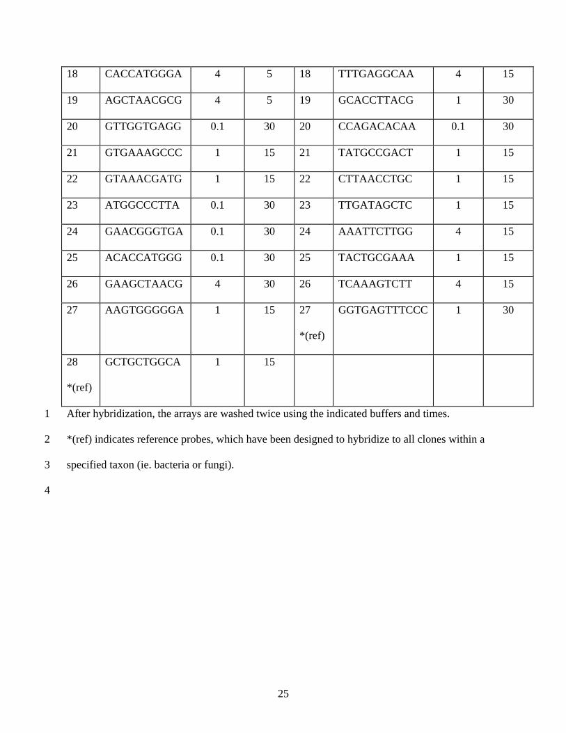
Table 1. Probe sequences and array washing conditions. 1
Bacteria Fungi
Probe
No.
Probe
Sequence
Washing
Buffer
(X SSC)
Washing
Time
(min)
Probe
No.
Probe
Sequence
Washing
Buffer
(X SSC)
Washing
Time
(min)
1 GTTGGGTTAA 0.1 30 1 ATAGGGATAG 1 30
2 GTAACCTGCC 1 30 2 CTGGCTTCTT 1 30
3 GAAAGCCTGA 1 30 3 GTCTTTGGGT 1 30
4 AATTCGATGC 1 30 4 GATTTGTCTG 4 15
5 TTCGGATTGT 1 30 5 AGGGATCGGG 0.1 30
6 CGAAAGCGTG 4 5 6 GCTACACTGA 0.1 30
7 CGGCCCAGAC 4 5 7 AAATAGCCCG 4 15
8 TTGATCCTGG 4 5 8 CGGTTCTATT 1 30
9 CACATGCAAG 1 30 9 TGATAGCTCT 1 30
10 GGTAATGGCC 1 30 10 CGCGCGCTAC 1 30
11 GGGCGCAAGC 1 30 11 GTTGGTGGAG 0.1 30
12 TGAAATGCGT 1 30 12 CTGGGTAATC 0.1 30
13 ATTCGATGCA 4 15 13 AATCAAAGTC 1 15
14 GCAAGCCTGA 4 30 14 GCCGTTCTTA 0.1 30
15 TCAGTTCGGA 1 30 15 GGCTTCTTAG 1 30
16 GAGGATGGCC 1 15 16 CAGAGCCAGC 0.1 30
17 GGGTAAAGGC 4 15 17 CAGACATAAC 1 15
25
18 CACCATGGGA 4 5 18 TTTGAGGCAA 4 15
19 AGCTAACGCG 4 5 19 GCACCTTACG 1 30
20 GTTGGTGAGG 0.1 30 20 CCAGACACAA 0.1 30
21 GTGAAAGCCC 1 15 21 TATGCCGACT 1 15
22 GTAAACGATG 1 15 22 CTTAACCTGC 1 15
23 ATGGCCCTTA 0.1 30 23 TTGATAGCTC 1 15
24 GAACGGGTGA 0.1 30 24 AAATTCTTGG 4 15
25 ACACCATGGG 0.1 30 25 TACTGCGAAA 1 15
26 GAAGCTAACG 4 30 26 TCAAAGTCTT 4 15
27 AAGTGGGGGA 1 15 27
*(ref)
GGTGAGTTTCCC 1 30
28
*(ref)
GCTGCTGGCA 1 15
After hybridization, the arrays are washed twice using the indicated buffers and times. 1
*(ref) indicates reference probes, which have been designed to hybridize to all clones within a 2
specified taxon (ie. bacteria or fungi). 3
4