3. Linear Regression With a Single Regressor

Econometrics: (I)

• Application of statistical methods in empirical research

• Testing economic theory with real-world data(data analysis)

56

Econometrics: (II)

• Econometric tasks:

1. Economic model

Specification:functional form (A assumptions)error term (B assumptions)variables (C assumptions)

2. Econometric model

Estimation

57

Econometrics: (III)

3. Model estimation

hypothesis testingprediction

Data:

• We need ”good” data in empirical economics

• Collecting data often poses practical problems(historical data vs. statistical experiments)

• No general (systematic) instructions

58

Types of data sets:

• Longitudinal data(observations on distinct entities at a given point of time)

• Time-series data(observations on a single entity observed at multiple pointsof time)

• Panel data(observations on distinct entities observed at multiple pointsof time)

59

Meaning of the notion ”regression”:

• Specification and analysis of a functional (parametric) rela-tionship between a dependent (endogenous) variable y and aset of independent (exogenous) variables

• 1 exogenous variable (x)

−→ regression with a single regressor

• k exogenous variables (x1, . . . , xk)

−→ regression with multiple regressors(see Section 4)

60

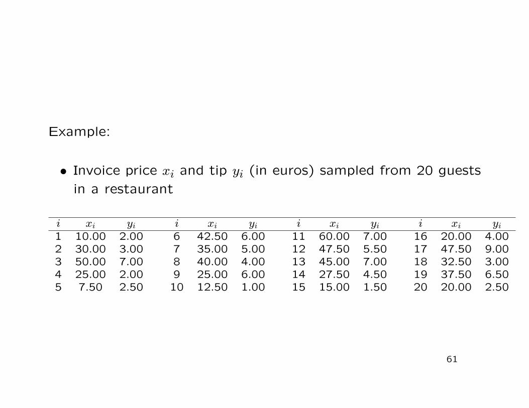
Example:

• Invoice price xi and tip yi (in euros) sampled from 20 guestsin a restaurant

i xi yi i xi yi i xi yi i xi yi1 10.00 2.00 6 42.50 6.00 11 60.00 7.00 16 20.00 4.002 30.00 3.00 7 35.00 5.00 12 47.50 5.50 17 47.50 9.003 50.00 7.00 8 40.00 4.00 13 45.00 7.00 18 32.50 3.004 25.00 2.00 9 25.00 6.00 14 27.50 4.50 19 37.50 6.505 7.50 2.50 10 12.50 1.00 15 15.00 1.50 20 20.00 2.50

61

3.1 Model Specification

1. Functional form (A assumptions)

Specification in 3 steps:

• Step #1: y = f(x), here: y = α + βx(’True’ relationship between invoice price x and tip y)

62

0

2

4

6

8

0 20 60 8040

Invoice price

Tip

Iy

x

20

20

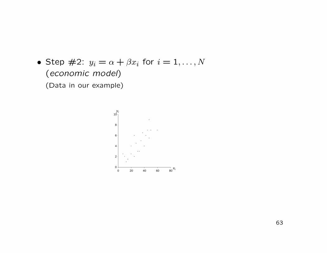
• Step #2: yi = α + βxi for i = 1, . . . , N(economic model)(Data in our example)

63

10y i

8

6

4

2

0 0 20 40 60 80 xi

• Step #3: yi = α + βxi + ui for i = 1, . . . , N(econometric model)

Remarks:

• We call α and β regression parameters or coefficients

• The random variable ui constitutes an error term

64

The A assumptions:

• Assumption #A1:Our econometric model does not lack of any further relevantexogenous variables beyond xi and the included exogenousvariable xi is not irrelevant

• Assumption #A2:The true relationship between xi and yi is linear

• Assumption #A3:The coefficients α and β are constant for all N observations(xi, yi)

65

2. Specification of the error term (B assumptions)

Rationale for the error term:

• Sampling and measurement errors

• Omitted exogenous variables

• Human behavior

66

The B assumptions:• Assumption #B1:

For i = 1, . . . , N we have

E(ui) = 0

• Assumption #B2:For i = 1, . . . , N we have

Var(ui) = σ2

• Assumption #B3:For i = 1, . . . , N and j = 1, . . . , N (i 6= j) we have

Cov(ui, uj) = 0

• Assumption #B4:The error terms ui are normally distributed, i.e. ui ∼ N(0, σ2)

67

Illustration of the B assumptions

68

3. Specification of the variables (C assumptions)

The C assumptions:

• Assumption #C1:The exogenous regressor xi is deterministic (not a randomvariable) and can be controlled in an experiment

• Assumption #C2:The regressor xi is not constant for all i = 1, . . . , N(i.e. there is variation among the xi’s)

69

3.2 (Point)Estimation

Until now:

• Specification of the econometric model

yi = α + βxi + ui

Now:

• Derivation of estimators α and β of the unknown parametersα und β via the Ordinary Least Squares (OLS) method

70

To this end:

• Distinction between ’true’ and ’estimated sphere’

• True econometric model

yi = α + βxi + ui

• Corresponding estimated model

yi = α + βxi

(after having derived ’appropriate estimators’ α and β)

−→ notion ’residual’

71

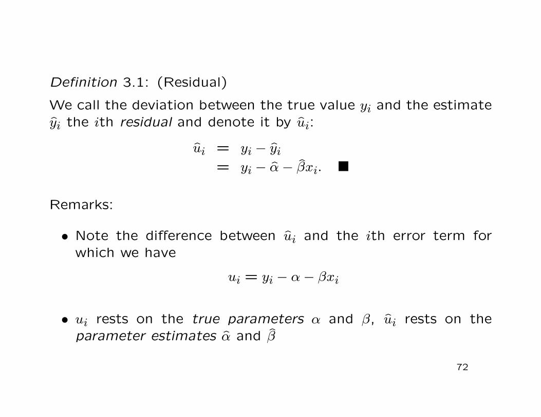
Definition 3.1: (Residual)

We call the deviation between the true value yi and the estimateyi the ith residual and denote it by ui:

ui = yi − yi= yi − α− βxi.

Remarks:

• Note the difference between ui and the ith error term forwhich we have

ui = yi − α− βxi

• ui rests on the true parameters α and β, ui rests on theparameter estimates α and β

72

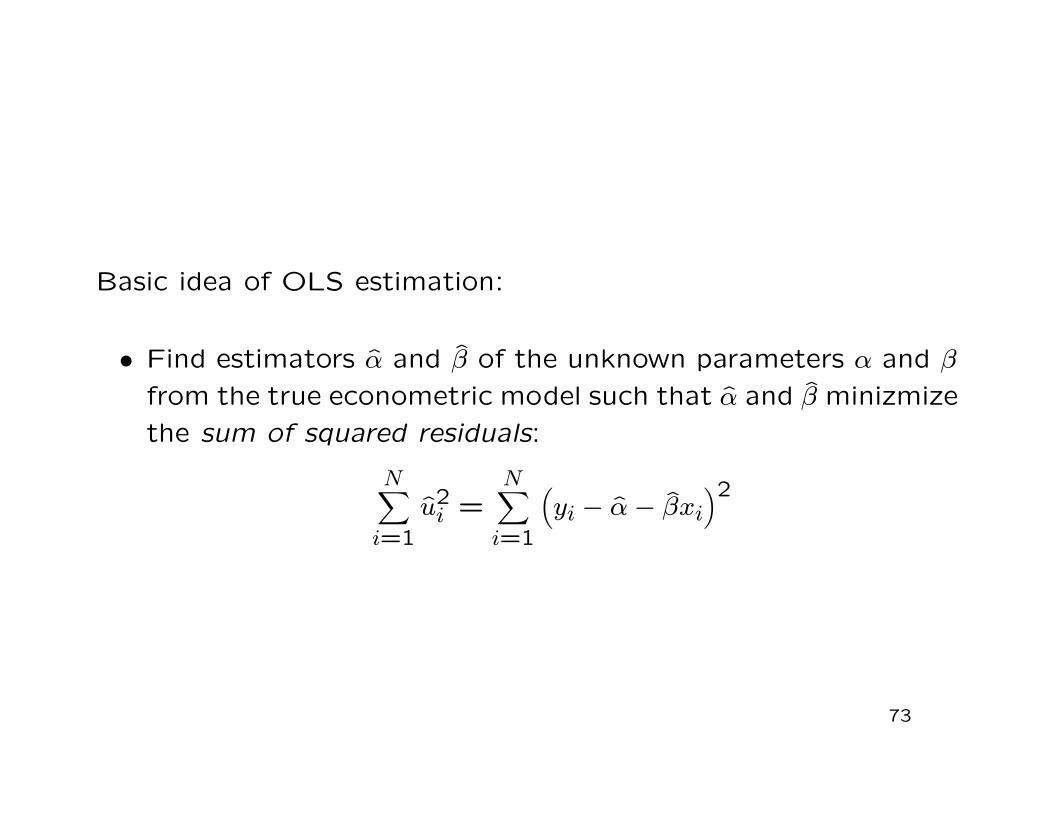
Basic idea of OLS estimation:

• Find estimators α and β of the unknown parameters α and βfrom the true econometric model such that α and β minizmizethe sum of squared residuals:

N∑

i=1u2

i =N∑

i=1

(

yi − α− βxi)2

73

Theorem 3.2: (OLS estimators)

In linear regression model with a single regressor

yi = α + βxi + ui, i = 1, . . . , n,

the Ordinary Least Squares (OLS) estimators are given by

β =

N∑

i=1(xi − x)(yi − y)

N∑

i=1(xi − x)2

,

α = y − βx.

(Proof: Class)

74

Remarks:

• The OLS estimators are formally derived by

partial differentiation of the sum of squared residuals withrespect to α, β

setting the partial derivatives equal to zero

solving the system of equations for α and β

• The assumption #B4, postulating normally distributed errorterms, is not needed in deriving the OLS estimators

75

Example: (Tip) (I)

• x =120

20∑

i=1xi = 31.50, y =

120

20∑

i=1yi = 4.45

•20∑

i=1(xi − x)2 = 4130,

20∑

i=1(xi − x)(yi − y) = 519

−→ β = 519/4130 = 0.125666

−→ α = 4.45− 0.125666 · 31.50 = 0.491521

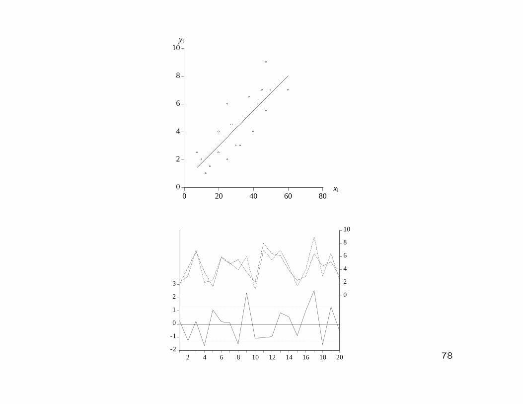
• Estimated model:

yi = 0.491521 + 0.125666 · xi

76

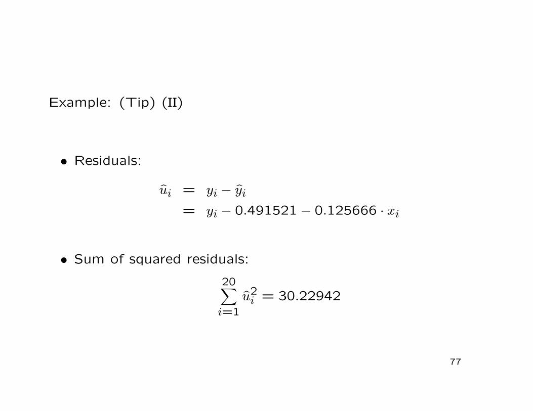
Example: (Tip) (II)

• Residuals:

ui = yi − yi

= yi − 0.491521− 0.125666 · xi

• Sum of squared residuals:

20∑

i=1u2

i = 30.22942

77

78

10yi

-2

-1

0

1

2

3

0

2

4

6

8

10

2 4 6 8 10 12 14 16 18 20

0

2

4

6

8

0 20 40 60 80xi

For the (true) econometric model we have

E(yi) = E(α + βxi + ui)

= E(α) + E(βxi) + E(ui)

= α + βxi

and

Var(yi) = E{

[yi − E(yi)]2}

= E{

[yi − α− βxi]2}

= E(u2i )

= Var(ui) = σ2

79

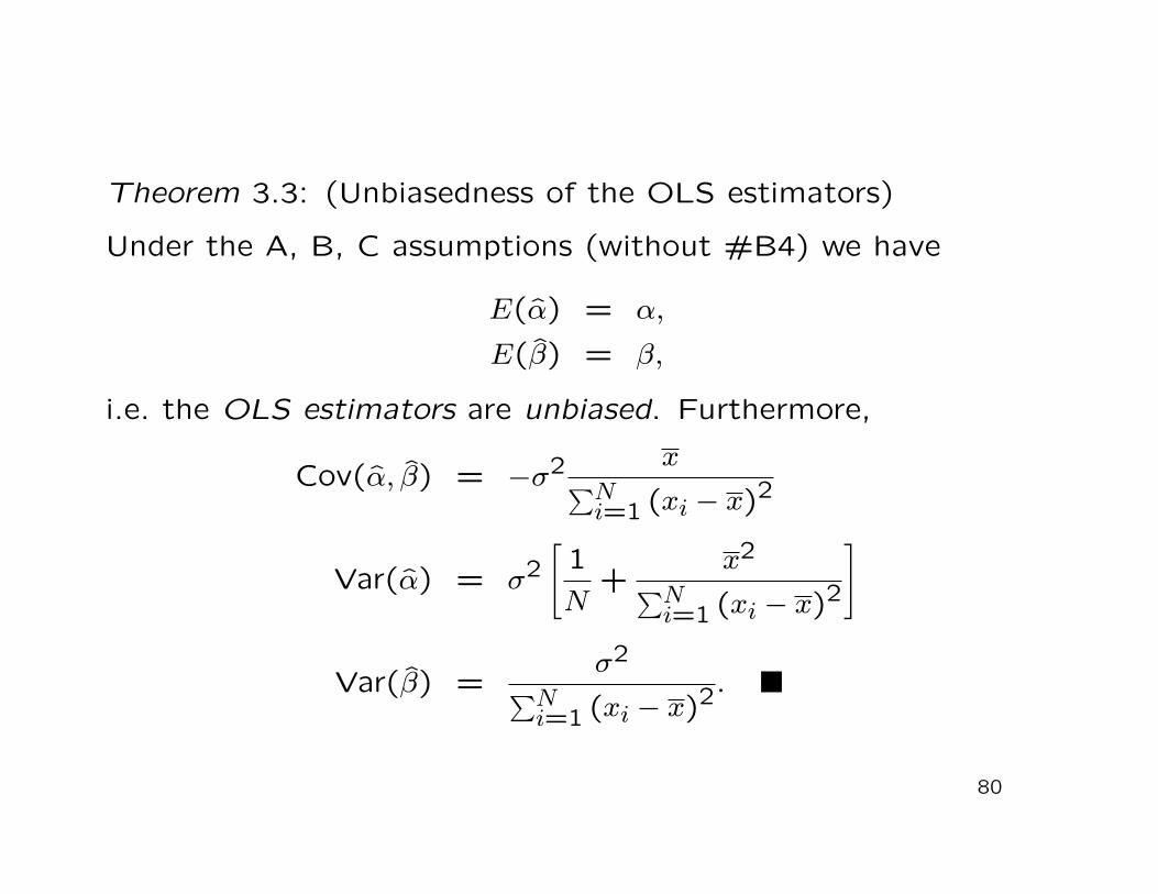
Theorem 3.3: (Unbiasedness of the OLS estimators)

Under the A, B, C assumptions (without #B4) we have

E(α) = α,

E(β) = β,

i.e. the OLS estimators are unbiased. Furthermore,

Cov(α, β) = −σ2 x∑N

i=1 (xi − x)2

Var(α) = σ2[

1N

+x2

∑Ni=1 (xi − x)2

]

Var(β) =σ2

∑Ni=1 (xi − x)2

.

80

Theorem 3.4: (Gauß-Markov-Theorem)

(a) Under the A, B, C assumptions (without #B4) the OLSestimators α and β have minimal variance among all linearand unbiased estimators of α and β.(BLUE = Best Linear Unbiased Estimators)

(b) Additionally, if the normality assumption #B4 for the errorterms ui holds, then the OLS estimators α and β have mini-mal variance among all unbiased estimators of α and β.(UMVUE = Uniformly minimum-variance unbiased estima-tors)

81

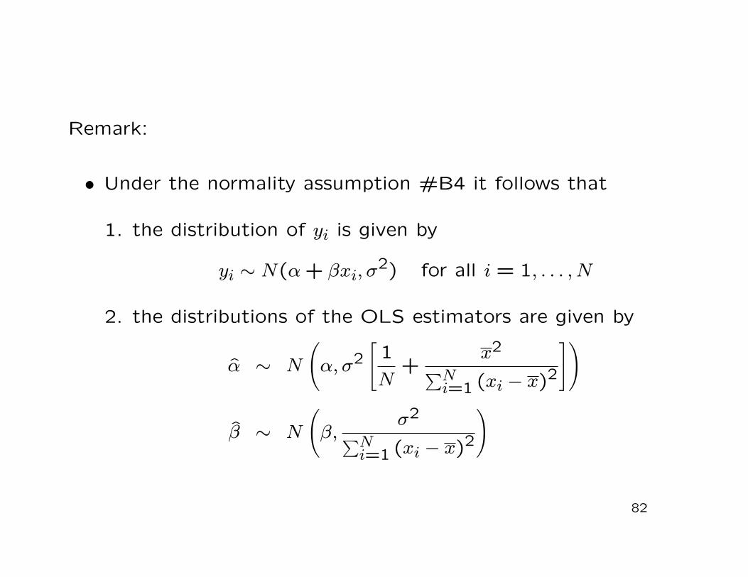
Remark:

• Under the normality assumption #B4 it follows that

1. the distribution of yi is given by

yi ∼ N(α + βxi, σ2) for all i = 1, . . . , N

2. the distributions of the OLS estimators are given by

α ∼ N

(

α, σ2[

1N

+x2

∑Ni=1 (xi − x)2

])

β ∼ N

(

β,σ2

∑Ni=1 (xi − x)2

)

82

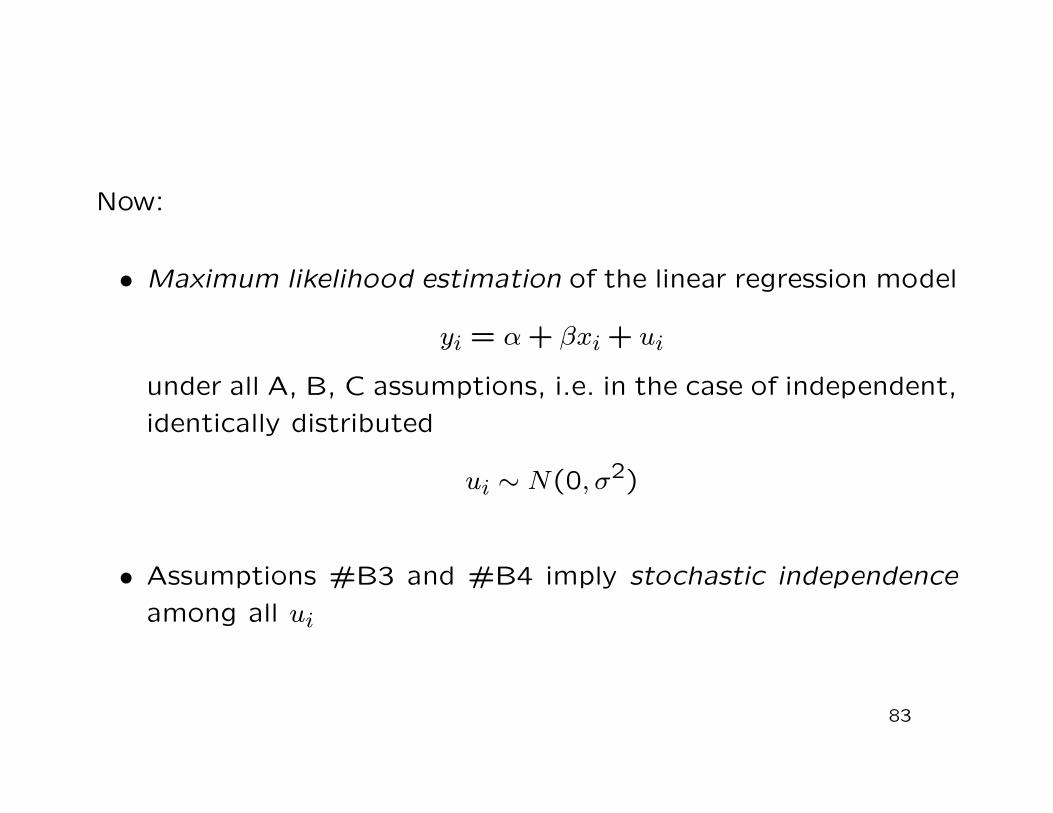
Now:

• Maximum likelihood estimation of the linear regression model

yi = α + βxi + ui

under all A, B, C assumptions, i.e. in the case of independent,identically distributed

ui ∼ N(0, σ2)

• Assumptions #B3 and #B4 imply stochastic independenceamong all ui

83

Derivation: (I)

• yi is a linear function of ui

−→ yi are independent with

yi ∼ N(α + βxi, σ2)

• The probability density function of yi is given by

fyi(y) =1√2πσ

exp

{

−12

[y − α− βxiσ

]2}

84

Derivation: (II)

• The joint density of the endogenous yi is given by

fy1,...,yN(y1, . . . , yN) =N∏

i=1fyi(yi)

=N∏

i=1

1√2πσ

exp

{

−12

[yi − α− βxiσ

]2}

=1

(2πσ2)N/2 exp

−1

2σ2

N∑

i=1(yi − α− βxi)

2

• The likelihood function is given by

L(α, β, σ2) =1

(2πσ2)N/2 exp

−1

2σ2

N∑

i=1(yi − α− βxi)

2

85

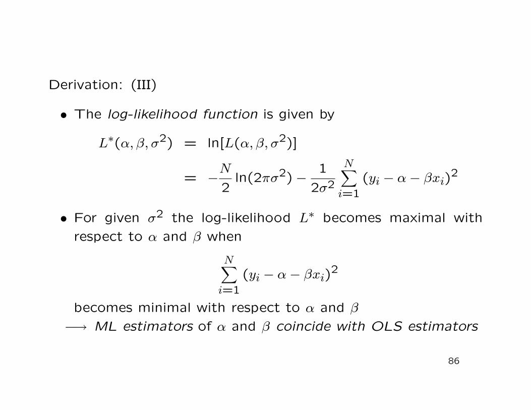
Derivation: (III)

• The log-likelihood function is given by

L∗(α, β, σ2) = ln[L(α, β, σ2)]

= −N2

ln(2πσ2)−1

2σ2

N∑

i=1(yi − α− βxi)

2

• For given σ2 the log-likelihood L∗ becomes maximal withrespect to α and β when

N∑

i=1(yi − α− βxi)

2

becomes minimal with respect to α and β−→ ML estimators of α and β coincide with OLS estimators

86

Derivation: (IV)

• Differentiating L∗ with respect to σ2 yields

∂ L∗

∂ σ2 = −N2

12πσ22π +

1(2σ2)2

2N∑

i=1(yi − α− βxi)

2

= −N

2σ2 +1

2σ4

N∑

i=1(yi − α− βxi)

2

• Setting the latter term equal to zero and inserting the MLestimators of α, β, we obtain

−N

2σ2ML

+1

2σ4ML

N∑

i=1

(

yi − αML − βMLxi)2

︸ ︷︷ ︸

= u2i

= 0

87

Derivation: (V)

• Solving for σ2ML, we find the ML estimator of σ2:

σ2ML =

1N

N∑

i=1u2

i

Remarks:

• The ML estimator σ2ML is biased:

E(

σ2ML

)

=N − 2

Nσ2

• Thus, an unbiased estimator of σ2 is given by

σ2 =N

N − 2σ2

ML =1

N − 2

N∑

i=1u2

i

88

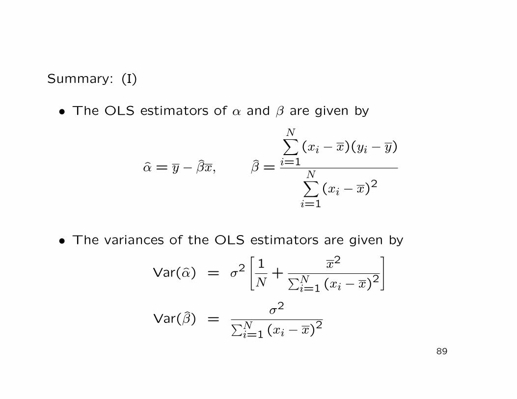
Summary: (I)

• The OLS estimators of α and β are given by

α = y − βx, β =

N∑

i=1(xi − x)(yi − y)

N∑

i=1(xi − x)2

• The variances of the OLS estimators are given by

Var(α) = σ2[

1N

+x2

∑Ni=1 (xi − x)2

]

Var(β) =σ2

∑Ni=1 (xi − x)2

89

Summary: (II)

• An unbiased estimator of σ2 is given by

σ2 =N

N − 2σ2

ML =1

N − 2

N∑

i=1u2

i

−→ standard errors of the OLS estimators

90

Definition 3.5: (Standard errors of the OLS estimators)

Replacing the unknown σ2 in the variance formulae of the OLSestimators α and β given in Theorem 3.3 (Slide 80) by the un-biased estimator

σ2 =1

N − 2

N∑

i=1u2

i

and taking the square root, we obtain the so called standarderrors of the OLS estimators:

SE(α) =

√

√

√

√σ2[

1N

+x2

∑Ni=1 (xi − x)2

]

,

SE(β) =

√

√

√

√

σ2∑N

i=1 (xi − x)2.

91

Remark:

• The standard error of an estimator is an estimator of thestandard deviation of the estimator and thus constitutes animportant measure of the precision of the estimator

92

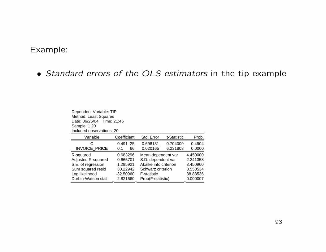
Example:

• Standard errors of the OLS estimators in the tip example

93

Dependent Variable: TIP Method: Least Squares Date: 06/25/04 Time: 21:46 Sample: 1 20 Included observations: 20

Variable Coefficient Std. Error t-Statistic Prob.

0.491 25 0.698181 0.704009 0.4904CINVOICE_PRICEICE 0.1 66 0.020165 6.231803 0.0000

4.4500002.2413583.450960

0.683296 Mean dependent var 0.665701 S.D. dependent var 1.295921 Akaike info criterion 30.22942 Schwarz criterion 3.550534

-32.50960 F-statistic 38.83536

R-squared Adjusted R-squared S.E. of regression Sum squared resid Log likelihood Durbin-Watson stat 2.821560 Prob(F-statistic) 0.000007

Question:

• How does our model estimated by OLS

yi = α + βxi

fit the data?

−→ How can we measure the fit of our regression line?

−→ Coefficient of determination R2

94

Derivation:

• Variation of the endogenous yi

Syy ≡N∑

i=1(yi − y)2

• Sum of squared residuals and explained variation

Suu ≡N∑

i=1u2

i and Syy ≡N∑

i=1

(

yi − y)2

=N∑

i=1(yi − y)2

95

Theorem 3.6:

If the true relationship between the endogenous yi and the ex-ogenous xi is linear (i.e. if Assumption #A2 is satisfied), thenafter OLS estimation the following result holds:

Syy = Syy + Suu.

Remark:

• Via OLS estimation the entire variation in the yi observationscan be divided into 2 components:

1. the variation explained by the estimated model (i.e. by theestimated regression line) Syy

2. the unexplained variation of the estimated model Suu

96

Definition 3.7: (Coefficient of determination)

The coefficient of determination of a regression model, R2, isdefined as that portion of the entire variation in the yi obser-vations that are explained by the model (i.e. by the regressionline):

R2 =explained variation

entire variation=

Syy

Syy.

Remarks: (I)

• It follows from Theorem 3.6 that

R2 =Syy

Syy=

Syy − SuuSyy

= 1−SuuSyy

97

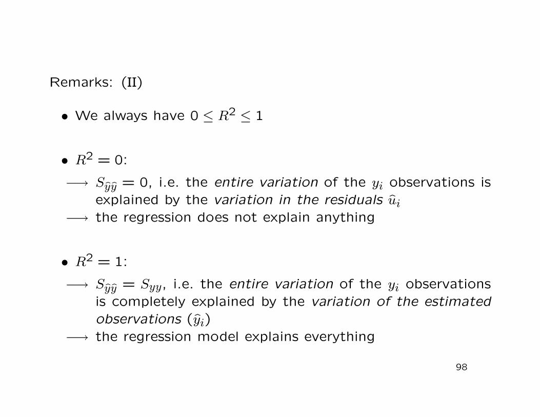
Remarks: (II)

• We always have 0 ≤ R2 ≤ 1

• R2 = 0:

−→ Syy = 0, i.e. the entire variation of the yi observations isexplained by the variation in the residuals ui

−→ the regression does not explain anything

• R2 = 1:

−→ Syy = Syy, i.e. the entire variation of the yi observationsis completely explained by the variation of the estimatedobservations (yi)

−→ the regression model explains everything

98

Remarks: (III)

• Direct computation of the R2 from the data (yi, xi):

R2 =βSxy

Syy=

S2xy

SxxSyy

=1

N2S2xy

1NSxx

1NSyy

=1

(N−1)2S2

xy1

N−1Sxx1

N−1Syy

(square of the sampling correlation coefficient)

99

3.3 Hypothesis Tests

Setting:

• Consider the linear regression model

yi = α + βxi + ui for i = 1, . . . , N,

with ui ∼ N(0, σ2)(Assumption #B4)

Now:

• Statistical hypothesis tests covering the parameter β

• One- and two-sided tests at the significance level a

100

Two-sided testing problem (q ∈ R):

H0 : β = q versus H1 : β 6= q

Appropriate test statistic:

T =β − qSE(β)

101

Reasoning: (I)• β − q is an estimator of the distance between β and q

• Estimator should be related to the dispersion (standard de-viation) of β:

SD(β) ≡√

Var(β) =

√

√

√

√

σ2∑N

i=1(xi − x)2

• Estimate SD(β) via the standard error SE(β)

SE(β) =

√

√

√

√

σ2∑N

i=1(xi − x)2

where

σ2 =1

N − 2

N∑

i=1u2

i

102

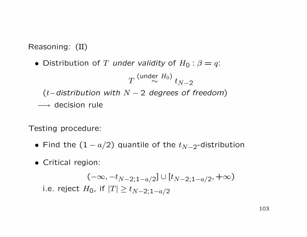
Reasoning: (II)

• Distribution of T under validity of H0 : β = q:

T(under H0)∼ tN−2

(t−distribution with N − 2 degrees of freedom)

−→ decision rule

Testing procedure:

• Find the (1− a/2) quantile of the tN−2-distribution

• Critical region:

(−∞,−tN−2;1−a/2] ∪ [tN−2;1−a/2,+∞)

i.e. reject H0, if |T | ≥ tN−2;1−a/2

103

104

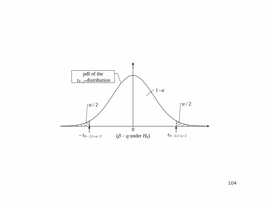
pdf of the tN 2-distribution

0 ( q under H0) tN ;1a

a / 2a / 2

a

tN ;1a

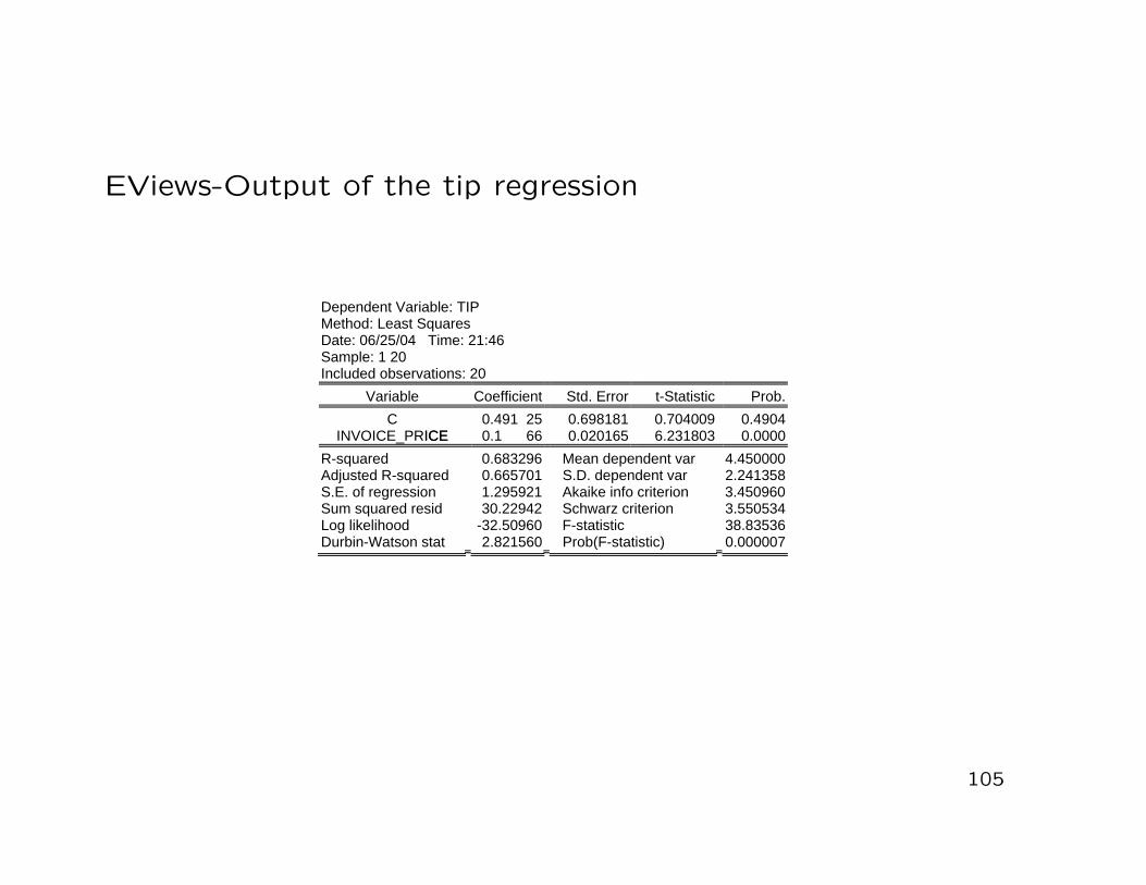
EViews-Output of the tip regression

105

Dependent Variable: TIP Method: Least Squares Date: 06/25/04 Time: 21:46 Sample: 1 20 Included observations: 20

Variable Coefficient Std. Error t-Statistic Prob.

0.491 25 0.698181 0.704009 0.4904CINVOICE_PRICEICE 0.1 66 0.020165 6.231803 0.0000

4.4500002.2413583.450960

0.683296 Mean dependent var 0.665701 S.D. dependent var 1.295921 Akaike info criterion 30.22942 Schwarz criterion 3.550534

-32.50960 F-statistic 38.83536

R-squared Adjusted R-squared S.E. of regression Sum squared resid Log likelihood Durbin-Watson stat 2.821560 Prob(F-statistic) 0.000007

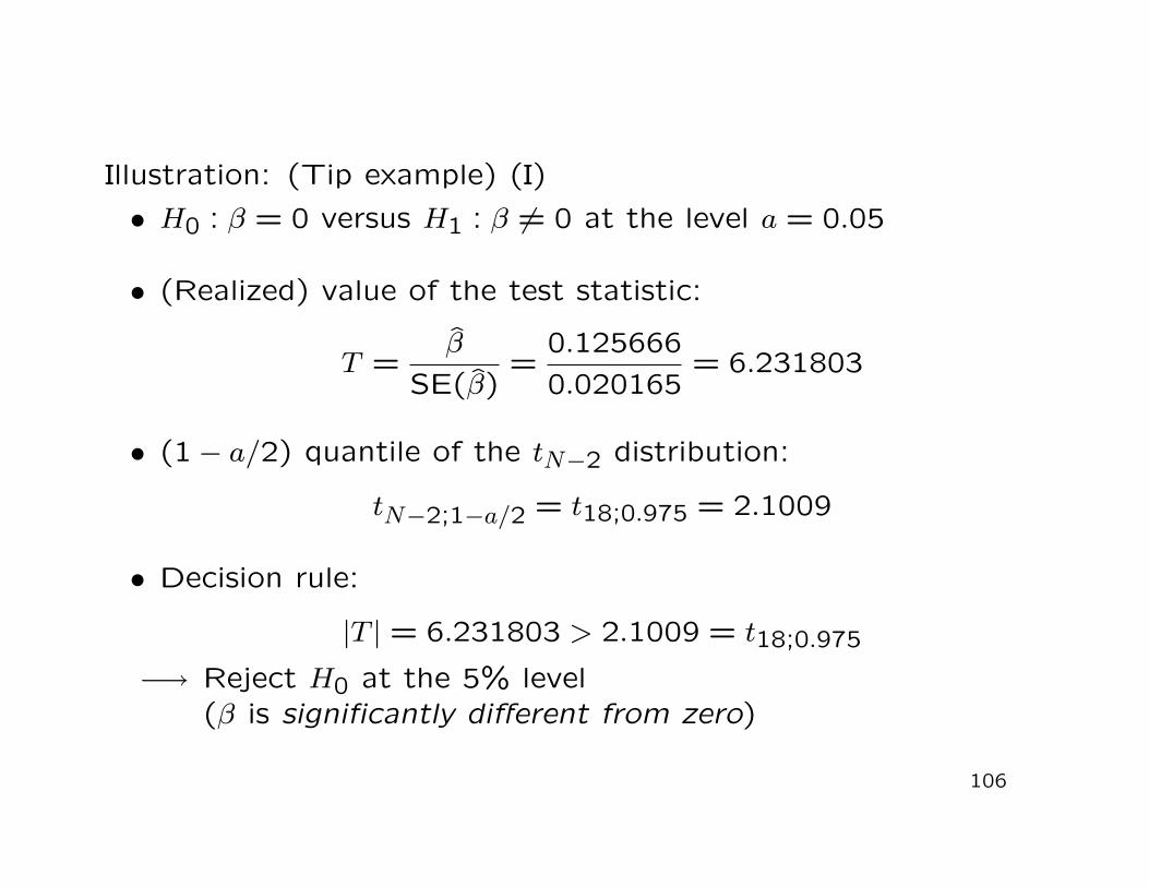
Illustration: (Tip example) (I)

• H0 : β = 0 versus H1 : β 6= 0 at the level a = 0.05

• (Realized) value of the test statistic:

T =β

SE(β)=

0.1256660.020165

= 6.231803

• (1− a/2) quantile of the tN−2 distribution:

tN−2;1−a/2 = t18;0.975 = 2.1009

• Decision rule:

|T | = 6.231803 > 2.1009 = t18;0.975

−→ Reject H0 at the 5% level(β is significantly different from zero)

106

Question:

• Is β significantly different from 0.1 (at the level a = 0.05)?

Testing procedure: (I)

• H0 : β = 0.1 versus H1 : β 6= 0.1 at the level a = 0.05

• (Realized) value of the test statistic:

T =β − 0.1SE(β)

=0.0256660.020165

= 1.272799

107

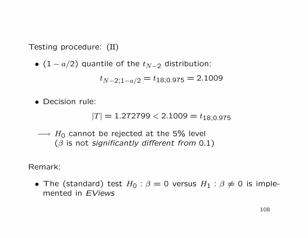
Testing procedure: (II)

• (1− a/2) quantile of the tN−2 distribution:

tN−2;1−a/2 = t18;0.975 = 2.1009

• Decision rule:

|T | = 1.272799 < 2.1009 = t18;0.975

−→ H0 cannot be rejected at the 5% level(β is not significantly different from 0.1)

Remark:

• The (standard) test H0 : β = 0 versus H1 : β 6= 0 is imple-mented in EViews

108

Now:

• One-sided hypothesis test at the level a

H0 : β ≤ q versus H1 : β > q

Conjecture behind this test:

• Invoice price has a positive impact on tip

Appropriate test statistic:

T =β − qSE(β)

109

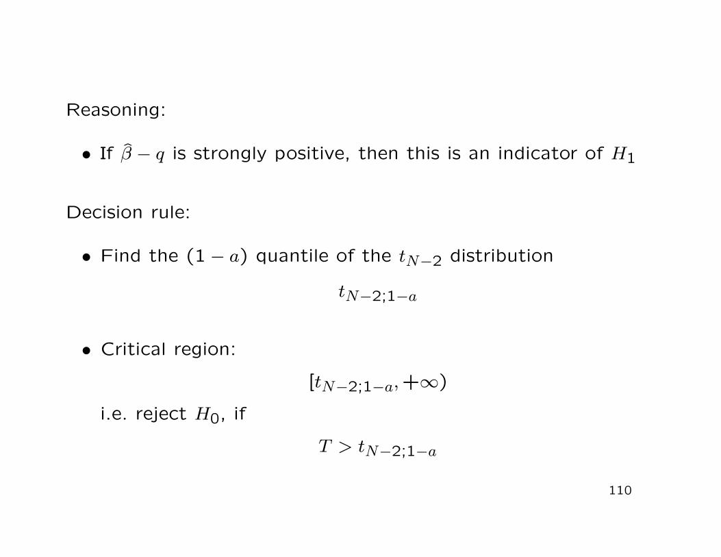
Reasoning:

• If β − q is strongly positive, then this is an indicator of H1

Decision rule:

• Find the (1− a) quantile of the tN−2 distribution

tN−2;1−a

• Critical region:

[tN−2;1−a,+∞)

i.e. reject H0, if

T > tN−2;1−a

110

Illustration: (Tip example)

• H0 : β ≤ 0.1 versus H1 : β > 0.1 at the level a = 0.05

• (Realized) test statistic:

T =β − 0.1SE(β)

=0.0256660.020165

= 1.272799

• (1− a) quantile of the tN−2 distribution:

tN−2;1−a = t18;0.95 = 1.7341

• Decision rule:

|T | = 1.272799 < 1.7341 = t18;0.95

−→ H0 cannot be rejected at the 5% level

111

Now:

• Important concept with regard to hypothesis testing witheconometric software−→ p-value

Classical procedure:

• Fix the significance level a (very often: a = 0.05)

• Find the critical region (i.e. find the quantiles of the H0-distribution of the test statistic) via the fixed significancelevel a

• Conduct this concrete test with a sample and decide at thelevel a between rejection and non-rejection of H0

112

Alternative procedure:

• Do not fix the significance level a, but instead consider a asvariable

• Conduct the concrete test with a sample and obtain therealization of the test statistic T

• On the basis of the critical region (i.e. use the quantiles ofthe H0-distribution of T ) find the lowest significance levelamin for which the concrete realization t just permits therejection of H0

113

Definition 3.8: (p-value)

The smallest significance level amin, for which the observed valuet of the test statistic T just permits the rejection of the nullhypothesis H0, is called the p-value.

114

Pdf of the tN 2-distribution

tN ;1a

T = t

0 ( q under H0)

a / 2a / 2

a

tN ;1a tN ;1amin

Example:

• Consider the test problem

H0 : β = q versus H1 : β 6= q

• Decision rule: reject H0 if

|T | ≥ tN−2;1−a/2

(cf. Slides 101–103)

• Assume that the realization of the test statistic T is t

• Find the p-value amin such that

|t| = tN−2;1−amin/2

115

Obviously:

• If H0 is rejected at the level amin, then H0 is also rejected atany other significance level a > amin−→ the lower the p-value amin, the higher the ’statistical jus-

tification’ of rejecting H0

• If the p-value amin < 0.05 then H0 can be rejected at the 5%level

• In our tip example the p-value of the coefficient β is

amin = 0.0000

(cf. Slide 105)−→ the null hypothesis H0 : β = 0 can be rejected at any

conventional significance level

116

3.4 Prediction

Now:

• Conditional prediction of the endogenous value y0 given theexogenous value x0

Forecast via the OLS estimators:

y0 = α + βx0

117

Illustration: (Tip example)

• Suppose that x0 = 20 euros

• Estimated model:

yi = 0.491525 + 0.125666xi

−→ conditional forecast

y0 = 3.004845

118

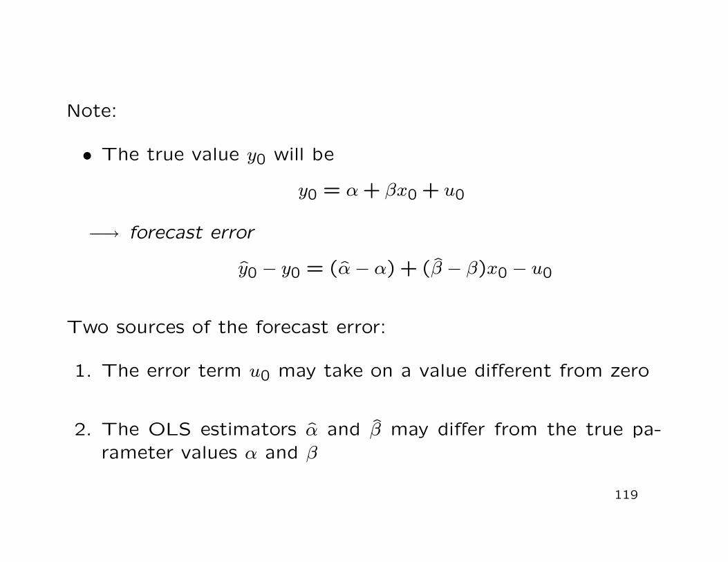
Note:

• The true value y0 will be

y0 = α + βx0 + u0

−→ forecast error

y0 − y0 = (α− α) + (β − β)x0 − u0

Two sources of the forecast error:

1. The error term u0 may take on a value different from zero

2. The OLS estimators α and β may differ from the true pa-rameter values α and β

119

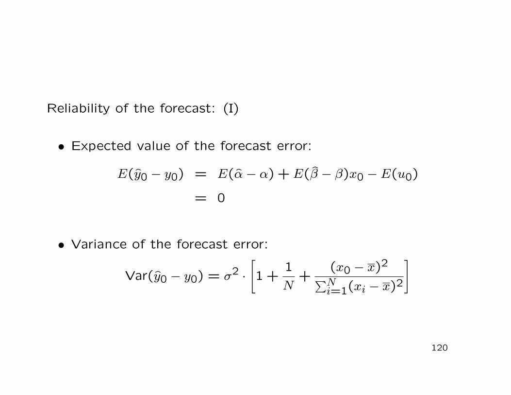
Reliability of the forecast: (I)

• Expected value of the forecast error:

E(y0 − y0) = E(α− α) + E(β − β)x0 − E(u0)

= 0

• Variance of the forecast error:

Var(y0 − y0) = σ2 ·[

1 +1N

+(x0 − x)2

∑Ni=1(xi − x)2

]

120

Reliability of the forecast: (II)

• Estimated variance of the forecast error:

Var(y0 − y0) = σ2 ·[

1 +1N

+(x0 − x)2

∑Ni=1(xi − x)2

]

where

σ2 = 1/(N − 2)N∑

i=1u2

i

(cf. Slide 91)

• Standard error of the forecast error:

SE(y0 − y0) =√

Var(y0 − y0)

121

Illustration: (Tip example) (I)

• For x0 = 20 the forecast is y0 = 3.004845

• The expected value of the forecast error is 0

• The OLS regression yields:

σ2 = (1.295921)2, x = 31.50,N∑

i=1(xi − x)2 = 4130

(cf. Output on Slides 105, 76)

122

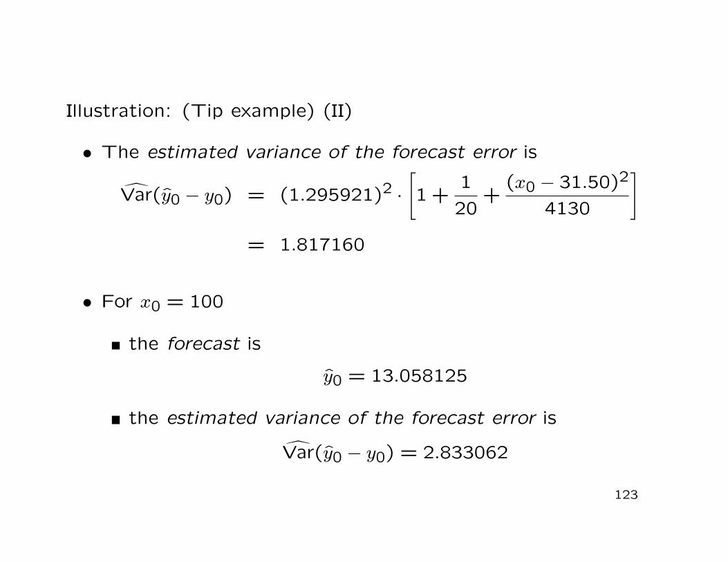
Illustration: (Tip example) (II)

• The estimated variance of the forecast error is

Var(y0 − y0) = (1.295921)2 ·[

1 +120

+(x0 − 31.50)2

4130

]

= 1.817160

• For x0 = 100

the forecast is

y0 = 13.058125

the estimated variance of the forecast error is

Var(y0 − y0) = 2.833062

123

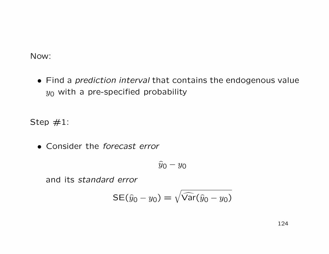
Now:

• Find a prediction interval that contains the endogenous valuey0 with a pre-specified probability

Step #1:

• Consider the forecast error

y0 − y0

and its standard error

SE(y0 − y0) =√

Var(y0 − y0)

124

Step #2:

• Standardization of the forecast error

T =(y0 − y0)−

=0︷ ︸︸ ︷

E (y0 − y0)SE(y0 − y0)

• It can be shown that

T ∼ tN−2

(t-distribution with N − 2 degrees of freedom)

125

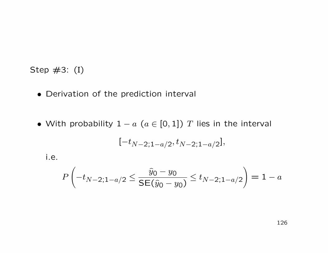
Step #3: (I)

• Derivation of the prediction interval

• With probability 1− a (a ∈ [0,1]) T lies in the interval

[−tN−2;1−a/2, tN−2;1−a/2],

i.e.

P

(

−tN−2;1−a/2 ≤y0 − y0

SE(y0 − y0)≤ tN−2;1−a/2

)

= 1− a

126

Step #3: (II)

• Solving for y0 we obtain

P{

y0 − tN−2;1−a/2 · SE(y0 − y0) ≤ y0

≤ y0 + tN−2;1−a/2 · SE(y0 − y0)}

= 1− a

• Thus, the prediction interval is given by

[y0 − tN−2;1−a/2 · SE(y0 − y0), y0 + tN−2;1−a/2 · SE(y0 − y0)]

127

Illustration: (Tip example)

• For x0 = 20 the forecast is

y0 = 3.004845

• The estimated variance is

Var(y0 − y0) = 1.402215

−→ for a = 0.05 the prediction interval is given by

[0.517061,5.492629]

128

Width of the prediction interval for y0 given x0

129

yi 0)y0 tN2;1a / 2 SE( y0 y

y0 tN 2;1a / 2 SE( y0 y0)

x0y0

x0