3. the rational expectations revolutionsweet.ua.pt/afreitas/aulas/notas...
TRANSCRIPT

Politicas macroeconomicas, handout, Miguel Lebre de Freitas ([email protected])
1
04/10/2017 http://sweet.ua.pt/afreitas/aulas/notas%20apoio/notasmacro.htm
3. The Rational Expectations Revolution
Index:
3. The Rational Expectations Revolution ......................................................................1
3.1 Introduction........................................................................................3 3.2 The worker misperception model ......................................................4
3.2.1 Main assumptions ......................................................................................4
3.2.2 Labour market equilibrium ........................................................................5
3.2.3 Aggregate supply .......................................................................................5
Box 3.1. The Phillips curve....................................................................................7
3.2.4 Equilibrium of the model ...........................................................................9
3.2.5 Inflation surprise ........................................................................................9
3.2.6 Short run and long run .............................................................................10
3.3 The model with backward looking expectations .............................11
3.3.1 Adaptive expectations..............................................................................11
3.3.2 Monetary surprise ....................................................................................12
3.3.3 Surprising and surprising again ...............................................................13
Box 3.2. Adaptive expectations and the accelerationist hypothesis ....................14
3.3.4 Summing up .............................................................................................15
3.4 Rational expectations .......................................................................16
3.4.1 Perfect foresight .......................................................................................17
3.4.2 Rational expectations and forecasting errors ...........................................17
3.4.3 The policy ineffectiveness proposition ....................................................18
Box 3.3: Only surprises matter! ...........................................................................19
3.4.4 The call for a Real Business Cycles Theory ............................................20
3.4.5 The slope of the supply curve ..................................................................21
Box 3.3. The Lucas critique.................................................................................22
3.4.6 Unpredictable outcomes...........................................................................23
3.5 Rules versus discretion ....................................................................25
3.5.1 The central banker’ objective function ....................................................25
3.5.2 Central bank’ optimum under discretion .................................................26
3.5.3 Inconsistency (under discretion) ..............................................................27
3.5.4 Consistency (under discretion) ................................................................28

Politicas macroeconomicas, handout, Miguel Lebre de Freitas ([email protected])
2
04/10/2017 http://sweet.ua.pt/afreitas/aulas/notas%20apoio/notasmacro.htm
3.5.5 Rules and other remedies .........................................................................29
3.5.6 The role of policy.....................................................................................29
3.6 The new Keynesian response...........................................................30
3.6.1 Staggered wages.......................................................................................30
3.6.2 Anticipated changes do matter.................................................................31
Box 3.4. The staggered wages model ..................................................................33
3.6.3 Policy implications...................................................................................34
3.7 Further reading.................................................................................35
Review questions and exercises...................................................................................36
Review questions .........................................................................................36 Problems ......................................................................................................36
Politicas macroeconomicas, handout, Miguel Lebre de Freitas ([email protected])
3
04/10/2017 http://sweet.ua.pt/afreitas/aulas/notas%20apoio/notasmacro.htm
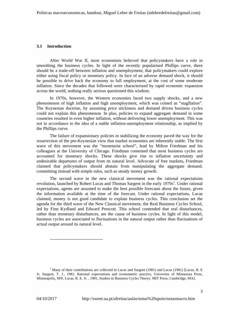
3.1 Introduction
After World War II, most economists believed that policymakers have a role in smoothing the business cycles. In light of the recently popularised Phillips curve, there should be a trade-off between inflation and unemployment, that policymakers could explore either using fiscal policy or monetary policy. In face of an adverse demand shock, it should be possible to drive back the economy to full employment, at the cost of some moderate inflation. Since the decades that followed were characterized by rapid economic expansion across the world, nothing really serious questioned this wisdom.
In 1970s, however, the Western economies faced two supply shocks, and a new phenomenon of high inflation and high unemployment, which was coined as “stagflation”. The Keynesian doctrine, by assuming price stickiness and demand driven business cycles could not explain this phenomenon. In plus, policies to expand aggregate demand in some countries resulted in even higher inflation, without delivering lower unemployment. This was not in accordance to the idea of a stable inflation-unemployment relationship, as implied by the Phillips curve.
The failure of expansionary policies in stabilizing the economy paved the way for the resurrection of the pre-Keynesian view that market economies are inherently stable. The first wave of this movement was the “monetarist school”, lead by Milton Friedman and his colleagues at the University of Chicago. Friedman contented that most business cycles are accounted for monetary shocks. These shocks give rise to inflation uncertainty and undesirable departures of output from its natural level. Advocate of free markets, Friedman claimed that policymakers should abstain from manipulating the aggregate demand, committing instead with simple rules, such as steady money growth.
The second wave in the new classical movement was the rational expectations revolution, launched by Robert Lucas and Thomas Sargent in the early 1970s1. Under rational expectations, agents are assumed to make the best possible forecasts about the future, given the information available at the time of the forecast. Under rational expectations, Lucas claimed, money is not good candidate to explain business cycles. This conclusion set the agenda for the third wave of the New Classical movement, the Real Business Cycles School, led by Finn Kydland and Edward Prescott. This school contended that real disturbances, rather than monetary disturbances, are the cause of business cycles. In light of this model, business cycles are associated to fluctuations in the natural output rather than fluctuations of actual output around its natural level.
1 Many of their contributions are collected in Lucas and Sargent (1981) and Lucas (1981) [Lucas, R. E Jr, Sargent, T. J., 1981, Rational expectations and econometric practice, University of Minnesota Press, Minneapolis, MN; Lucas, R. E. Jr. , 1981, Studies in Business Cycles Theory. MIT Press, Cambridge, MA].

Politicas macroeconomicas, handout, Miguel Lebre de Freitas ([email protected])
4
04/10/2017 http://sweet.ua.pt/afreitas/aulas/notas%20apoio/notasmacro.htm
The modelling innovations introduced by the New Classical School inspired a new generation of economists aligned with the Keynesian tradition. These economists developed macroeconomic models grounded with microeconomic foundations, but with different types of market failures, to argue that the price mechanism is too slow, even under rational expectations. Since the market mechanism fails in delivering full employment, it is argued, there is scope for the central bank to stabilize the economy.
This note briefly reviews these ideas, focusing on the key assumption of Rational Expectations. In Section 2, we introduce the workers’ misperception model, which will be used to explain how information failures may give rise to departures of output away from its natural level. In Section 3, we describe the case with backward looking expectations. In Section 4 we solve the same model assuming instead that agents are rational. In Section 5, we illustrate how rational expectations weighed on the debate “rules versus discretion”. In Section 6, we briefly explain how earlier New Keynesian theories, by adding price stickiness to the model, re-established the effectiveness of monetary policy, even under rational expectations. To keep things simple, the explanation is more intuitive than formal. Technical details are addressed in boxes.
3.2 The worker misperception model
3.2.1 Main assumptions
Consider a closed economy with perfect competition where prices and wages are flexible. In this economy, production takes place using two factors of production, labour and capital. The capital stock is pre-determined and equal to 1.
For simplicity, let’s consider a Cob-Douglass production function: 1zNQ (3.1)
Firms take productivity (z), the output price (P), and the nominal wage rate (W) as given and choose the number of workers so as to maximize profits. Assuming perfect competition, this problem delivers the well known optimality condition stating that the demand for labour is such that the marginal product of labour equals the real wage. Solving for N, this gives:
1
1
W
PzN d (3.2)
The implied supply function is obtained replacing (3.2) in (3.1):
1
1 1W
PzQs (3.3)
The novelty in this model is that workers do not observe the price level at the time they make their decisions: workers set their nominal wages taking into account the real wage they aim to receive, and the expected price level, eP .

Politicas macroeconomicas, handout, Miguel Lebre de Freitas ([email protected])
5
04/10/2017 http://sweet.ua.pt/afreitas/aulas/notas%20apoio/notasmacro.htm
For simplicity, let’s assume that the supply of labour is infinitely elastic at the desired real wage, . Formally, our labour supply function will be as follows:
ePW (3.4)
In this model, firms have an information advantage over workers: firms know the price at which they are selling their own output. Workers, however, are concerned with the consumer price index. The consumer price index is an average of all consumer prices, and hence not readily available. Thus, workers will not immediately notice when the price level changes. This is why nominal wages (in 3.4) are set based on an expectation of what the price level will be.
3.2.2 Labour market equilibrium
Given (3.2) and (3.4), the equilibrium in the labour market is given by:
1*
eP
PNN , with
1
* 1
zN (3.5)
Equation (3.5) reveals that the equilibrium employment in this economy depends on the gap between expected prices and actual prices. In case there are no information frictions ( ePP ), the economy will operate at its “natural rate of employment”, *N , just like in a classical world. When prices are higher than expected, workers will still supply labour at the agreed nominal wage, because they do not immediately acknowledge the fall in real wage. Firms, in turn, will demand more labour because they observe the real wage declining.
As long as the expected price does not change, equation (3.5) implies a positive relationship between employment and prices, which basically accords to the Phillips curve (see Box 3.1). The novelty in the model with expectations is that changes in the later destabilize the relationship between employment and prices.
3.2.3 Aggregate supply
In this model, the price level only influences output to the extent that it is different from expected. Replacing (3.5) in (3.1), the general expression of aggregate supply in this model is:
1
*eP
PQQ with
11
* 1zQ (3.6)
Where *Q refers to “natural output”.

Politicas macroeconomicas, handout, Miguel Lebre de Freitas ([email protected])
6
04/10/2017 http://sweet.ua.pt/afreitas/aulas/notas%20apoio/notasmacro.htm
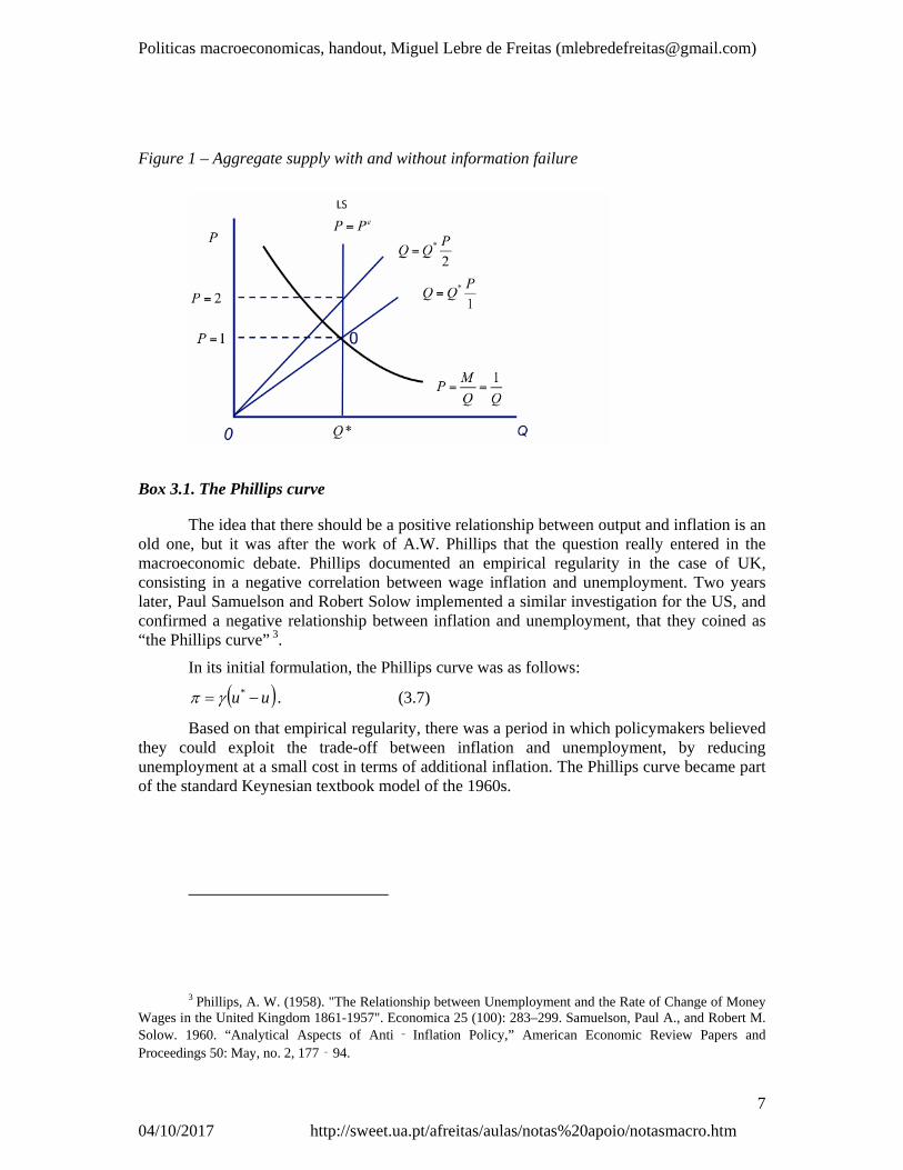
Equation (3.6) is known as the “Friedman-Lucas supply function”. It describes a family of aggregate supply curves, each one corresponding to a given expected price, eP . Along each curve, when the price level increases, firms produce more output because real wages decline2.
To illustrate the model with a simple numerical example, in what follows we refer to the following parameterization: 1z , 5.0 , and 5.0 . This delivers the convenient
benchmark: 1** QN , and the supply curve becomes simply:
eP
PQ (3.6a)
In Figure 1, we depict two aggregate supply curves (AS), corresponding to this parameterisation: one for 1eP and other 2eP . The frictionless case correspond to LS (for Long-term Supply), where output is at its natural level.
2 The split of the economy into firms and workers is a matter of expositional convenience. One could
instead think of different agents trading with each other different products. This was the approach followed by Lucas [Lucas, R. , 1972. Expectations and the neutrality of money. Journal of Economic Theory, 4, 103-24]. While the Friedman model - sketched out above - emphasises fooling workers, the Lucas version of the model emphasizes an information barrier shared by workers and firms alike: in the Lucas model all agents are labelled as “firms”, which sell different products in competitive markets and have no control over their own price. Firms observe changes in their own prices, but information barriers prevent them from correctly asserting how much of these are accounted for by industry-specific shocks or instead by aggregate demand shocks. Thus, depending on how firms expect the general price level to evolve, they will respond to price changes by producing more or less. Although the micro paradigm is different from the one use by Friedman, the implied aggregate supply function is the same. The advantage of the Lucas formulation is that it doesn’t rely on a negative correlation between output and real wages, which is empirically refuted.
Politicas macroeconomicas, handout, Miguel Lebre de Freitas ([email protected])
7
04/10/2017 http://sweet.ua.pt/afreitas/aulas/notas%20apoio/notasmacro.htm
Figure 1 – Aggregate supply with and without information failure
Box 3.1. The Phillips curve
The idea that there should be a positive relationship between output and inflation is an old one, but it was after the work of A.W. Phillips that the question really entered in the macroeconomic debate. Phillips documented an empirical regularity in the case of UK, consisting in a negative correlation between wage inflation and unemployment. Two years later, Paul Samuelson and Robert Solow implemented a similar investigation for the US, and confirmed a negative relationship between inflation and unemployment, that they coined as “the Phillips curve” 3.
In its initial formulation, the Phillips curve was as follows:
uu * . (3.7)
Based on that empirical regularity, there was a period in which policymakers believed they could exploit the trade-off between inflation and unemployment, by reducing unemployment at a small cost in terms of additional inflation. The Phillips curve became part of the standard Keynesian textbook model of the 1960s.
3 Phillips, A. W. (1958). "The Relationship between Unemployment and the Rate of Change of Money
Wages in the United Kingdom 1861-1957". Economica 25 (100): 283–299. Samuelson, Paul A., and Robert M. Solow. 1960. “Analytical Aspects of Anti ‐ Inflation Policy,” American Economic Review Papers and Proceedings 50: May, no. 2, 177‐94.

Politicas macroeconomicas, handout, Miguel Lebre de Freitas ([email protected])
8
04/10/2017 http://sweet.ua.pt/afreitas/aulas/notas%20apoio/notasmacro.htm
This view was strongly criticized by Milton Friedman. In his 1968 presidential address to the American Economic Association, Friedman criticized the Phillips curve on the grounds that it neglected the role of expectations 4.
Friedman then proposed the “expectations-augmented” Phillips curve, given as follows:
euu * . (3.7a)
In terms of the model above, the “expectations-augmented” Phillips curve corresponds to the supply function (3.6), but in a log-linear version of the model. Formally, one must first substitute (3.4) in (3.1) and take logs, obtaining:
wpzq
1ln
1ln
1 (3.3a)
where lowercase letters denote the logarithms of the corresponding uppercase variables.
The linear equation equivalent to (3.4) is: epw ln , (3.4a)
Replacing (3.4a) in (3.3a), we get:
eppqq
1* (3.6b)
where
ln1ln1ln1* zq .
Adding and subtracting 1p to the term in brackets in (3.6b) and defining 1 pp ,
and 1 ppee we get:
*
1qqe
(3.7b)
Mediating (3.7b) and the Phillips curve (3.7a) there is another stylized fact, known as the Okun’s Law. The Okun’s Law says that the distance between the actual and the “natural rate of unemployment” is a negative function of the distance between actual and natural output. Formally, this is ** uuqq . Replacing in the equation above, we get (3.7a).
As we can infer from the model, the initial formulation of the Phillips curve (3.7) would only be possible in a world in which workers were concerned with nominal wages (instead of real wages). In that case, it would be possible for monetary policy to change relative prices in a permanent manner, giving rise to real effects. In the more realistic case in
4 Milton Friedman (1968). “The Role of Monetary Policy”. American Economic Review, 58, 1-17.
Politicas macroeconomicas, handout, Miguel Lebre de Freitas ([email protected])
9
04/10/2017 http://sweet.ua.pt/afreitas/aulas/notas%20apoio/notasmacro.htm
which agents are concerned with real wages, nominal variables are set according to expected changes in the consumer price index. Thus, the entire Phillips curve shifts upwards when expected inflation increases (eq. 3.7a).
3.2.4 Equilibrium of the model
In line with the classical tradition, let’s assume that the quantitative theory of money holds, and that money velocity is equal to 1. Hence, aggregate demand is given by the money market equilibrium:
PQM (3.8)
The two main equations of the model are aggregate supply (3.6) and aggregate demand, (3.7). Solving these two equations together, one obtains the equilibrium levels of output and of prices:
*
1
Q
MPP e (3.9)
1*
eP
MQQ (3.10)
For instance, when M=1 and 1eP , we have P=1 and *QQ . This particular equilibrium is described by point 0 in Figure 1.
3.2.5 Inflation surprise
Returning to Figure 1, suppose that our economy is initially in a frictionless equilibrium, with M=1 and 1 ePP (point 0). Then, assume that the money supply unexpectedly shifts, once-and-for-all, to M=4. The increase in money supply gives rise to an increase in the price level, but workers are still expecting the price level to be equal to one. The fact that the price level increases ahead of expectations causes the real wage rate to decline, employment to increase, and output to expand above full employment.
The equilibrium in the output market following the monetary surprise is described by point 1 in Figure 2. This point corresponds to the intersection of the new aggregate demand,
PQ4 , with the aggregate supply with 1eP , PQ , implying .2QP

Politicas macroeconomicas, handout, Miguel Lebre de Freitas ([email protected])
10
04/10/2017 http://sweet.ua.pt/afreitas/aulas/notas%20apoio/notasmacro.htm
Figure 2 – Equilibrium in the output market following an inflation surprise
The reason underlying the shift in output ahead of full employment is that firms, observing the fall in real wage, optimally decide to hire more labour. This is illustrated in Figure 3: because the price level doubled, real wages halved. Hence, firms increased their demand for labour, hiring N=4 and therefore expanding production to Q=2.
Figure 3 – Equilibrium in the labour market following the inflation surprise
It is important to note that in point 1 workers are out of their labour supply. However, workers will only perceive this in a later stage, when the information regarding the price level becomes available. In this model, the labour market clears “ex ante”: wages are set such that the labour market is expected to clear. However, the labour market does not necessarily clear “ex post”. The labour market clears in expectations only. With this reasoning, one can generate departures from full employment, even in a context where prices are flexible.
3.2.6 Short run and long run
The main idea behind this model is that agents may lack all the information they need to accurately make their economic decisions. In particular, people may not perceive a change in the price level caused by a monetary shock. Thus, even if wages are inherently flexible,

Politicas macroeconomicas, handout, Miguel Lebre de Freitas ([email protected])
11
04/10/2017 http://sweet.ua.pt/afreitas/aulas/notas%20apoio/notasmacro.htm
agents may fail to adjust their labour contracts, departing from their optimal paths. In the aggregate, this results in fluctuations of output around its natural rate.
Note that the equilibrium described in point 1 can only occur in the short run. Sooner of later, workers will catch on to the fact that their purchasing power has declined. The expected price will be revised upwards and a higher nominal wage rate will be demanded. Hence, the aggregate supply curve shifts upwards. In the long run, information failures vanish and the economy returns to its natural level (point T in Figure 2, Point 0 in Figure 3).
This is why in this model we have a short run aggregate supply (AS) and a long run aggregate supply (LS): in the long run, there are no information failures and the implied aggregate supply is vertical, mimicking the classical case.
The critical question is how long it will take for workers to correctly guess the price level:
- If the adjustment in expectations is slow, the business cycle will be long-lasting.
- If the adjustment in expectations is fast, the business cycle will be short-lived.
As we will see in a minute, these two cases mark the distinction between the initial assumption of backward looking expectations made by Milton Friedman and that of rational expectations, introduced by Robert Lucas.
3.3 The model with backward looking expectations
In a seminal paper, developed as part of its Presidential Address to the American Economic Association in 1967, Friedman offered an explanation to the apparent trade-off between inflation and unemployment underlying the Phillips curve. He contended that, because of information failures, monetary expansions cause output to expand ahead of its “natural level”. In the long run, however, there will be no trade-off between inflation and unemployment5. With this theory, Friedman re-stated the effectiveness of monetary policy in the short run and the classical proposition of money neutrality in the long run.
3.3.1 Adaptive expectations
The assumption of adaptive expectations presumes that agents collect information on the past values of a given variable and use this information to guess the future values of that
5 The same conclusion was independently discovered by Friedman and the Keynesian economist
Edmund Phelps: Friedman, M., 1968. The role of monetary policy. American Economic Review 58, 1-17. Phelps, Edmund S. “Phillips Curves, Expectations of Inflation and Optimal Employment over Time.” Economica, n.s., 34, no. 3 (1967): 254–281

Politicas macroeconomicas, handout, Miguel Lebre de Freitas ([email protected])
12
04/10/2017 http://sweet.ua.pt/afreitas/aulas/notas%20apoio/notasmacro.htm
variable. In our case, workers are assumed to guess future prices based on the prices observed in the past. The simpler model in this category is as follows:
1 PPe (3.11)
That is, workers expect this period’ prices to be equal to the level observed in the last period6.
3.3.2 Monetary surprise
Consider again the monetary surprise at time t=1, from M=1 to M=4.
At t=1, workers were expecting 11 eP , because this was the price level observed at t=0. Thus, the monetary shock causes the economy to move to point 1 in Figure 4, just like in Figure 2.
In moment t=2 workers expect 22 eP , because this is the price observed in t=1. In
Figure 4, this is described by the upward shift in the short term aggregate supply to 2PQ .
The new short term equilibrium (t=2) occurs in point 2, with 5.02 8P , and 5.0
2 2Q (see 3.9
and 3.10). Then, in period t=3, the worker will expect 5.03 8eP , implying a further upward
move in the aggregate supply, and so on.
Thus, even if money supply shifted once-and-for-all, the backward looking worker will be fooled and fooled again, until the final point T is reached.
6 This case is known as “naïve”, and is a particular case of “adaptive expectations”. With adaptive
expectations, the expected price each year is equal to the previous year expectation plus a “partial-adjustment”
term, correcting for the previous year’ forecasting error: eee PPPP 111 , with 10 . When 1
adaptive expectations can equivalently be written as a distributed lag of previous years prices, with weights
declining exponentially at rate 1 : jj
j
e PP 11 . The lower the value of , the greater the inertia
in expectations. When 0 , expectations are “myopic” and never revised (as implied by the original Phillips curve). When 1 , we have the “naïve model” above.

Politicas macroeconomicas, handout, Miguel Lebre de Freitas ([email protected])
13
04/10/2017 http://sweet.ua.pt/afreitas/aulas/notas%20apoio/notasmacro.htm
Figure 4 – Adjustment under adaptive expectations
In sum: the fact that workers gradually adapt their expectations implies that following a once-and-for-all shift in the money supply, output will take time to return to its natural level. Friedman contended that the process through which workers adjust their expectations can be “surprisingly long”. Meanwhile, a business cycle was generated7.
In the long run, however, the Quantitative Theory will show up and output will be independent of the price level: in the long run, there is no trade off between inflation and output, Friedman claimed. The absence of a long-term trade-off between inflation and unemployment seems to accord better with the evidence during the inflation years of the 1970s and the 1980s.
An implication of the model with adaptive expectations is that it is difficult to reduce inflation quickly without a significant increase in unemployment. In terms of our model, a sharp contraction in the money supply would give rise to an increase in real wages and low employment. Because workers are slow in adjusting expectations, output losses will persist over time. Under adaptive expectations, a gradualist policy, like a slow decline in the rate of money growth, looks like being the best strategy to reduce inflation.
3.3.3 Surprising and surprising again
The previous exercise relies on the assumption that the increase in money was once-and-for all. If money was allowed instead to expand every year, would it be possible to keep the economy operating above its natural employment level on a permanent basis?
7 Together with Anna Schwartz, Friedman wrote “A monetary history of the United States, 1867-
1960”. In this volume, the authors contended that business cycles in the US were mostly accounted for by changes in monetary conditions. They also contend that the Great Depression was the result of a “tragic policy mistake”: the decline in the money supply caused by bank failures could have been avoided by the Federal Reserve, and it wasn’t.

Politicas macroeconomicas, handout, Miguel Lebre de Freitas ([email protected])
14
04/10/2017 http://sweet.ua.pt/afreitas/aulas/notas%20apoio/notasmacro.htm
To answer this question, let’s consider again the main equations of our model, aggregate supply (3.6) and aggregate demand (3.8). Also consider the simple case in which
1** QN . Suppose that the monetary authorities were targeting the output level Q=2. How much should be the amount of money each year? Replacing (3.8) in (3.8), and using the assumption of adaptive expectations (3.7), one obtains
111
QM
QM
P
QMQ
Setting Q=2 every year, this gives
12 MM
That is, it would be possible to maintain output systematically above full employment, if money supply doubled each period. With such rule, prices would be increasing systematically ahead of wages, fooling the worker continuously.
Figure 5 illustrates the successive equilibria under the assumption that the monetary authorities are doubling money every period, surprising workers again and again.
Figure 5 –Demand pull inflation under static inflation expectations
Note that points 1, 2, and 3 define a Phillips curve corresponding to an expected inflation equal to zero (agents expect the price level to be the same as last year). Along the equilibria 1, 2, 3, however, prices double each year, implying an inflation rate of 100%. Since actual inflation is higher than expected inflation, output is above full employment. In Box 3.2 we show that the inflationary impact of the policy is even higher if workers form expectations in terms of inflation, rather than in terms of the price level.
Box 3.2. Adaptive expectations and the accelerationist hypothesis
In the examples above, we examined the implications of changes in the quantity of money on the price level. In the real world, however, the money supply expands every year, and people are concerned with inflation, not with the price level. The right tool to think the inflation-output trade off is the Phillips curve.
Politicas macroeconomicas, handout, Miguel Lebre de Freitas ([email protected])
15
04/10/2017 http://sweet.ua.pt/afreitas/aulas/notas%20apoio/notasmacro.htm
Friedman argued that attempts to keep unemployment low at the expense of higher inflation would result in higher inflation expectations. Friedman assumed that inflation expectations are formed adaptively. The “naïve” case is:
1 e (3.11a)
Replacing this in (3.7a), we get:
uu *
This equation suggests that it is possible to keep unemployment systematically below its natural rate, with an ever increasing inflation rate. An increasing inflation rate would allow prices to outpace wages each moment in time, fooling the workers again and again. This implication of the model is labelled the “acceleracionist hypothesis”.
To see the difference relative to the model in levels, note that the “naïve” expectation in prices (3.11) corresponds to a “myopic” expectation in terms of inflation: in Figure 5, along points 1, 2 and 3 expected inflation is always zero. Had people guess inflation in period 2 to be equal to that observed in period 1 and the AS curve would have shifted from Q=P in t=1 to Q=P/4 in t=2, determining lower output gap. Hence, if the government wanted output to remain at Q=2, it would need to accept an ever-increasing inflation rate. This is the accelerationist proposition.
When however the inflation rate is constant, the model delivers *uu . Using this model, Friedman introduced the concept of the NAIRU – the non-accelerating inflation rate of unemployment, *u 8.
3.3.4 Summing up
Keynes contented that output may deviate from full employment because of sticky prices. Focusing in the Great Depression, Keynes advocated that monetary policy was ineffective and fiscal policy should have been used. Friedman showed that it is possible to generate business cycles in a model where prices are flexible, because of information failures. In the scope of this model, Friedman restored the effectiveness of monetary policy, vut only in the short run: in the long run, the classical dichotomy holds.
As for the role of policy, Friedman was rather conservative: although the central bank has the power to expand economic activity, a question arises as whether such power should be used at all. Indeed, in the absence of monetary surprises, the economy will operate at its natural level, with workers getting the real wage they want. In contrast, under monetary instability, agents will depart from their supply curves and there will be undesirable fluctuations of output around its natural level. This observation, together with the claim that
8 Note however that when the unemployment rate is below the natural rate the inflation rate is
increasing, not accelerating: what is accelerating is the price level.

Politicas macroeconomicas, handout, Miguel Lebre de Freitas ([email protected])
16
04/10/2017 http://sweet.ua.pt/afreitas/aulas/notas%20apoio/notasmacro.htm
policymakers may lack the knowledge or the will to rightly implement stabilization policies9 led Friedman to defend that central banks should follow simple money supply rules, such as a setting the money supply to grow at a constant rate over time (hence, the label “monetarism”). With rules, surprises would be minimized and the economy should operate close to full employment.
3.4 Rational expectations
The assumption of adaptive expectations proposed by Friedman is a strong one. With adaptive expectations, agents are not given the possibility of processing optimally the information and learn with past mistakes. Referring to the example in Figure 4, one may question whether it would be reasonable to believe that, following the once-and-for-all shift in money supply, workers engage in a sequence of systematic forecasting errors all the way from 1 to T.
In alternative, Robert Lucas and Thomas Sargent proposed that agents should be rational 10 . Under rational expectations, people are forward-looking and make the best possible forecast given the all information they have. This is more than just using the past information on the forecasting variable. Under rational expectations, forecasts have to take into account what agents expect to happen in the future (agents are forward-looking), and they have to be formulated in consistency with the model describing the economy (rational expectations are model-consistent). In our model, people do not know exactly how much the central bank will expand the money supply (there is uncertainty), but they are aware of the mechanics through which changes in money supply affect prices.
More precisely, people are assumed to understand Figure 4 and be aware of equation (3.9). Thus, people will know that M=1 and 1eP imply P=1 (point 0); that 1eP and
M=4 imply P=2 (point 1); and that 2eP and M=4 imply 5.08P (point 2). With this model
in mind, people will realize that there is no point in guessing 2eP when M=4, because
9 First, governments may lack relevant information, such as the true value of multipliers and the natural
level of output. If, for instance, the natural output is overestimated, there is a risk of policymakers to engage in futile expansionary policies which only result is inflation. This is likely to have been the case in the early 1970s. Second, policy actions are effected by different types of lags, such as in the decision-making process, in implementation, and in the transmission to the real economy. Hence, the risk exist that, once the government starts to act and the effects of the policy are transmitted to the economy, the later is already on its way to full employment, risking more instability. Third, policy makers are influenced by lobbies, election calendars and other pressures. Hence, their actions may deviate too much from the public interest.
10 Lucas, R. , 1972, op. cit. Forward looking expectations had already been accounted for in the work of Edmund Phelps, though without rational expectations. Rational expectations were first proposed by John Muth, in 1962 (Rational expectations and the theory of price movements, Econometrica 29, 315-35).
Politicas macroeconomicas, handout, Miguel Lebre de Freitas ([email protected])
17
04/10/2017 http://sweet.ua.pt/afreitas/aulas/notas%20apoio/notasmacro.htm
such prediction would imply frustrated expectations. If people expect the money supply to be 4eM , the only “consistent” expectation is 4eP .
3.4.1 Perfect foresight
To better understand how the model works under rational expectations, let’s consider first the extreme case with no uncertainty: suppose that people know exactly where the aggregate demand curve each moment in time is. This case is labelled “perfect foresight”.
Referring to our previous exercise, if agents know that M=1 at t=0 and M=4 at t=1, people will rightly guess that 10 P and 41 P . Thus, the economy will immediately move
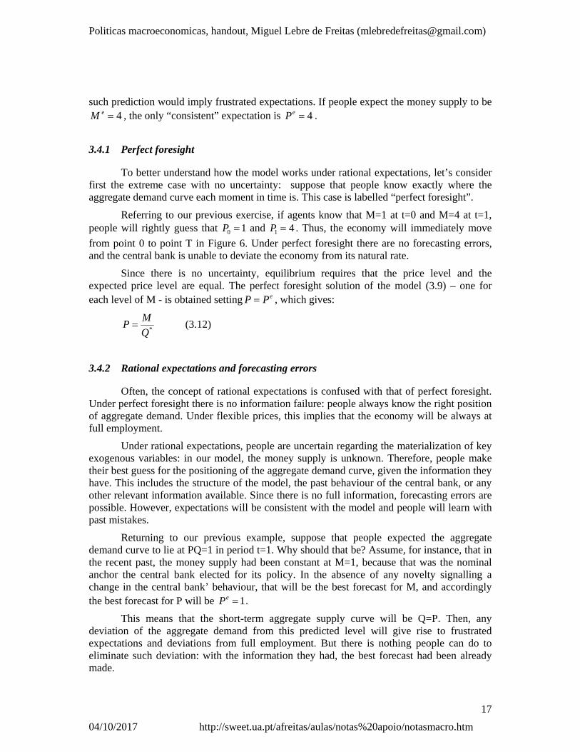
from point 0 to point T in Figure 6. Under perfect foresight there are no forecasting errors, and the central bank is unable to deviate the economy from its natural rate.
Since there is no uncertainty, equilibrium requires that the price level and the expected price level are equal. The perfect foresight solution of the model (3.9) – one for each level of M - is obtained setting ePP , which gives:
*Q
MP (3.12)
3.4.2 Rational expectations and forecasting errors
Often, the concept of rational expectations is confused with that of perfect foresight. Under perfect foresight there is no information failure: people always know the right position of aggregate demand. Under flexible prices, this implies that the economy will be always at full employment.
Under rational expectations, people are uncertain regarding the materialization of key exogenous variables: in our model, the money supply is unknown. Therefore, people make their best guess for the positioning of the aggregate demand curve, given the information they have. This includes the structure of the model, the past behaviour of the central bank, or any other relevant information available. Since there is no full information, forecasting errors are possible. However, expectations will be consistent with the model and people will learn with past mistakes.
Returning to our previous example, suppose that people expected the aggregate demand curve to lie at PQ=1 in period t=1. Why should that be? Assume, for instance, that in the recent past, the money supply had been constant at M=1, because that was the nominal anchor the central bank elected for its policy. In the absence of any novelty signalling a change in the central bank’ behaviour, that will be the best forecast for M, and accordingly the best forecast for P will be 1eP .
This means that the short-term aggregate supply curve will be Q=P. Then, any deviation of the aggregate demand from this predicted level will give rise to frustrated expectations and deviations from full employment. But there is nothing people can do to eliminate such deviation: with the information they had, the best forecast had been already made.
Politicas macroeconomicas, handout, Miguel Lebre de Freitas ([email protected])
18
04/10/2017 http://sweet.ua.pt/afreitas/aulas/notas%20apoio/notasmacro.htm
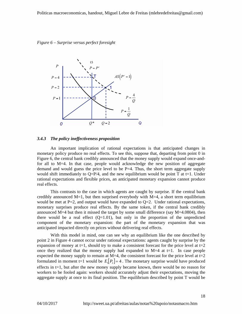
Figure 6 – Surprise versus perfect foresight
3.4.3 The policy ineffectiveness proposition
An important implication of rational expectations is that anticipated changes in monetary policy produce no real effects. To see this, suppose that, departing from point 0 in Figure 6, the central bank credibly announced that the money supply would expand once-and-for all to M=4. In that case, people would acknowledge the new position of aggregate demand and would guess the price level to be P=4. Thus, the short term aggregate supply would shift immediately to Q=P/4, and the new equilibrium would be point T at t=1. Under rational expectations and flexible prices, an anticipated monetary expansion cannot produce real effects.
This contrasts to the case in which agents are caught by surprise. If the central bank credibly announced M=1, but then surprised everybody with M=4, a short term equilibrium would be met at P=2, and output would have expanded to Q=2. Under rational expectations, monetary surprises produce real effects. By the same token, if the central bank credibly announced M=4 but then it missed the target by some small difference (say M=4.0804), then there would be a real effect (Q=1.01), but only in the proportion of the unpredicted component of the monetary expansion: the part of the monetary expansion that was anticipated impacted directly on prices without delivering real effects.
With this model in mind, one can see why an equilibrium like the one described by point 2 in Figure 4 cannot occur under rational expectations: agents caught by surprise by the expansion of money at t=1, should try to make a consistent forecast for the price level at t=2 once they realized that the money supply had expanded to M=4 at t=1. In case people expected the money supply to remain at M=4, the consistent forecast for the price level at t=2 formulated in moment t=1 would be 421 PE . The monetary surprise would have produced effects in t=1, but after the new money supply became known, there would be no reason for workers to be fooled again: workers should accurately adjust their expectations, moving the aggregate supply at once to its final position. The equilibrium described by point T would be
Politicas macroeconomicas, handout, Miguel Lebre de Freitas ([email protected])
19
04/10/2017 http://sweet.ua.pt/afreitas/aulas/notas%20apoio/notasmacro.htm
reached in moment t=2, and not after many periods, during which workers are systematically fooled by inconsistent guesses, as Friedman asserted.
The statement that anticipated changes in money have no effect on economic activity is known and the “policy ineffectiveness proposition” 11 . The policy ineffectiveness proposition does not rule out output effects from unexpected policy changes: monetary surprises will, in general, give rise to real effects. These real effects will be however short-lived, because people will rapidly adjust their expectations.
These conclusions have implications for the design of a disinflation programme. We saw that under adaptive expectations, a gradualist policy will in general come along with lower output costs than a policy that tries to reduce very sharply the inflation rate in a small period of time. With rational expectations, however, the story is different: what matters for the costs of a disinflation programme is the extent to which it is anticipated and people believe in it. This reasoning lead some authors to argue the society would be better off if the central bank followed a shock therapy (“cold turkey”), than trying to be smooth. The reason is that this would be credibility-enhancing, allowing agents to align faster their expectations with the policymaker intentions, delivering faster price adjustment and lower output costs.
Box 3.3: Only surprises matter!
To see how monetary surprises give rise to real effects in a model with inflation, let’s return to the linear version of our model, as described by equation (3.6b) plus a log version of (3.8):
pmq (3.8a)
Using (3.6b) and (3.8a), the log-linear equivalent to (3.9) and (3.10) are:
*11 qmpEp (3.9a)
pEmqq 1* 1 (3.10a)
In this formulation, we replaced ep by pE 1 to stress the fact that the expectation was formulated based on all the information available in the period before. Taking expectations based on the available information available at time t-1, we get:
*111 1 qmEpEpE
Solving for pE 1 , we obtain the rational expectations forecast:
*11 qmEpE (3.12a)
11 Sargent, Thomas & Wallace, Neil (1975). "'Rational' Expectations, the Optimal Monetary
Instrument, and the Optimal Money Supply Rule". Journal of Political Economy 83 (2): 241–254.

Politicas macroeconomicas, handout, Miguel Lebre de Freitas ([email protected])
20
04/10/2017 http://sweet.ua.pt/afreitas/aulas/notas%20apoio/notasmacro.htm
You may compare this equation to the solution of the model under perfect foresight (3.12): in the certainty case, the price level is proportional to money; in the case with imperfect information, the forecast of the price level has to be proportional to what people expect the money supply to be.
Substituting this back in (3.10a), one obtains:
mEmqq 1* 1 (3.13)
Denoting for the forecasting error, that is, the difference between the actual money supply and the expected money supply, we get:
1*qq
This equation shows that output only differs from its natural level to the extent that agents are surprised by unexpected increases in the money supply. When the money supply is correctly anticipated ( 0 ), then output will be at its natural level. Under rational expectations and flexible prices, only surprises produce real effects.
3.4.4 The call for a Real Business Cycles Theory
In our days, information lags regarding the consumer price index are very short-lived. Hence, any departure of actual output from its natural rate because of a monetary disturbance should be necessarily short-lived as well. With rational expectations and flexible prices, monetary policy can no longer be a good candidate to explain business cycles.
With such a conclusion, Lucas contended that economists should turn to explanations for the business cycles not relying on information failures and nominal shocks: If deviations from full employment output are so short-lived, economists should turn to explaining economic fluctuations in the context of flexible prices”. This was the agenda of the real business cycles theory12.
Proponents of the Real Business Cycles theory shifted the analysis away from information failures and monetary surprises, to focus on productivity shocks and other frictions that cause fluctuations of the natural rate of output, rather than fluctuations of actual output around its natural level. The real business cycles theory abstracts from information failures, postulating that the economy is always at full employment (the aggregate supply is vertical, even in the short run). Since productivity shocks tend to be persistent over time, the theory accounts for multiyear business cycles, without the need to rely on information lags.
12 “Kydland, Finn; E. C. Prescott (1982). "Time to Build and Aggregate Fluctuations". Econometrica
50 (6): 1345–1370. King, R. , Plosser, C., 1984. "Money, Credit, and Prices in a Real Business Cycle," American Economic Review, 74(3), 363-380.
Politicas macroeconomicas, handout, Miguel Lebre de Freitas ([email protected])
21
04/10/2017 http://sweet.ua.pt/afreitas/aulas/notas%20apoio/notasmacro.htm
3.4.5 The slope of the supply curve
As we just saw, once agents realize that the money supply shifted from a constant money rule at M=1 to a novel M=4 at moment t=1, they understand they need to revise their expectations. The best forecast implies, however, understanding the central bank’ intentions. Agents should ask: why did the central bank change the money supply? Was this a once-and-for-all move? Or instead this was marking a change in the monetary regime?
Consider for a moment that the announcement that the money supply shifted once-and-for-all to M=4 was credible. If agents get convinced that the central bank just adopted a new target at M=4, they will forecast 421 PE . In that case, the new AS curve will be
4PQ . Then, if the money supply M=4 actually materializes, there will be no more real effects.
For the central bank, this could constitute a lesson: looking at the initial AS curve, described by Q=P, the central bank might have acknowledged that this curve implied a given trade-off between inflation and output. The size of this trade-off relied however on a past experience of monetary stability: it is because money supply was stable until t=0 that the slope of the AS curve was as it was.
By unexpectedly expanding the money supply to M=4 at t=1, the central bank has explored the trade-off implied by the slope of the AS curve, producing P=2 and Q=2. In other words, an output gap amounting to 1* QQ was achieved with a price increase of 1P
(the relationship between *QQ and P can be interpreted as the slope of a Phillips curve). However, the real expansion lasted for one period only: once people realized that the new money supply had increased to M=4, they adjusted the expectations accordingly, rotating the AS curve upwards.
This example illustrates a key result in models with rational expectations: once policymakers try to explore the trade-off between inflation and unemployment implied by the slope of the aggregate supply, the slope changes. The initial slope of the AS curve reflected an earlier history of monetary stability. After the policy change, the AS supply curve became much steeper, implying that a higher inflation surprise will be needed to generate the same output expansion. In case people anticipate M to remain at M=4, the new AS curve will be
PQ 4 . Thus, the price level will need to increase from P=2 to P=8 ( 6P ) to generate a similar output expansion.
Of course, things will get even worse if people become suspicious about the intentions of the central bank: after all, it the central bank surprised everybody with M=4 when people were expecting M=1, why shouldn’t the central bank try to surprise again (setting M=16) after convincing everybody that M will remain equal to 4? Note in that case, in case people expect M=16, the aggregate supply curve jumps to Q=P/16, becoming even steeper: the lower the credibility of the central bank, the steeper will be the aggregate supply, implying that an even higher inflation will be needed to generate the same output expansion.
In sum: initially, the trust in monetary stability authorities created the potential for the central bank to explore the positive relation between prices and output implied by the short term aggregate supply curve. After this trade-off was explored, however, achieving the same output gap will require much higher increase in prices: as people learn with past mistakes, part of the monetary expansion will be anticipated and will impact directly on prices without

Politicas macroeconomicas, handout, Miguel Lebre de Freitas ([email protected])
22
04/10/2017 http://sweet.ua.pt/afreitas/aulas/notas%20apoio/notasmacro.htm
any real effect. Thus, a much higher inflation rate will be needed to achieve the same output gap. In other words, the Phillips curve becomes steeper.
With this reasoning, one may guess that an inflation surprise is likely to produce more real effects in the Euro Area than in Venezuela:
- In Venezuela, where inflation has been extremely volatile and high, a monetary expansion will hardly surprise agents, implying that the Phillips curve there is almost vertical.
- In contrast, in the Euro Area, where the past experience has been of monetary stability, the slope of the Phillips curve is moderate. This means that the ECB has the potential to expand output by creating an inflation surprise. The problem however is that once the monetary authorities try to explore the trade-off, the trade-off will dissipate: the Phillips curve will become steeper and steeper, approaching the limiting case of that in Venezuela.
All in all, although there is a potentially negative trade-off between inflation and unemployment, this trade-off rapidly disappears once the monetary authorities try to explore it.
Box 3.3. The Lucas critique
The changing slope of the Phillips curve is an illustration of a key implication of rational expectations: the statistical relationship between two variables may change when the policy changes, because expectations also change. This fact poses a serious limitation to the use of econometric models for policy formulation and forecasting. This argument is known as the Lucas Critique13.
To see this in terms of our model, let’s assume that the money supply has followed the stochastic process:
ttt mm 01 (3.14)
with being a white noise. In light of (3.14), the money supply has been increasing at the rate 0 (policy target), but there are unpredictable shocks, reflecting the central bank
inability to exactly control the money supply.
In that case, the best forecast for the money supply at moment t will be:
011 ttt mmE
13 Lucas, Robert (1976). "Econometric Policy Evaluation: A Critique". In Brunner, K.; Meltzer, A. The
Phillips Curve and Labor Markets. Carnegie-Rochester Conference Series on Public Policy 1. New York: American Elsevier. pp. 19–46.

Politicas macroeconomicas, handout, Miguel Lebre de Freitas ([email protected])
23
04/10/2017 http://sweet.ua.pt/afreitas/aulas/notas%20apoio/notasmacro.htm
People are aware that unpredictable shocks will cause the aggregate demand to vibrate around the expected position, given rise to real effects, but since these shocks are unpredictable this is the best forecast people can make.
Substituting this in (3.13), gives the following equation describing output:
10* 11 ttt mmqq (3.13a)
Note that (3.13a) is not different from (3.13): both say that only forecasting errors (materializations of ), produce deviations of output from full employment. In (3.13a), however, the equation for output is formulated in terms of the change in money supply, showing that the money rule together with the supply curve give rise to a statistical regularity involving the output gap, *qq , and the actual rate of money growth 1 tt mm .
If the central bank tried to estimate an equation for the output gap as a function of money creation, it would probably observe that changes in money have been associated to departures of output away from full employment. The estimated equation could be of the form:
tt mbaqq ˆˆ*
Based on the estimation results, the central bank could try to explore the relationship between output and money, changing the money rule to:
ttt mm 11 with 01 .
However, such a shift would only produce significant real effects at the very beginning. After people realize that the money rule has changed, they will guess
11 tt mm , and only the unpredictable error will matter again.
The important point to make is that the policy change altered a coefficient in the regression equation, in this case the intercept. With the change in expectations, the new relationship between output and money becomes 11
* 11 ttt mmqq ,
implying that the intercept of the regression equation changes to 11 a . Thus, once the policymaker used the econometric relationship for policy purposes, the econometric relationship has changed.
In sum: econometric estimates describe relationships between economic variables as they held in the past, under past policies. Whenever policy (the rules of the game) changes, the way people form expectations will also change. Hence, the parameters and elasticities estimated using past data will be a poor guide to what will happen in response to a policy change. This is the Lucas Critique.
3.4.6 Unpredictable outcomes
Under rational expectations, people learn with past mistakes. Hence, if the monetary authorities insist in expanding output ahead of its natural level, people will become aware of the central bank intentions, turning the central banks aim increasingly difficult to be achieved: in order to surprise and keep surprising, the central bank would need to be “incredibly imaginative”.

Politicas macroeconomicas, handout, Miguel Lebre de Freitas ([email protected])
24
04/10/2017 http://sweet.ua.pt/afreitas/aulas/notas%20apoio/notasmacro.htm
To illustrate this, we refer to Figure 7: will it be possible for a central banker facing rational agents to keep the economy operating at Q=2? In the figure, point 0 describes the initial situation in which 1 eMM , and point 1 describes the equilibrium after the
monetary authorities unexpectedly expanded money to M=4. The interesting question is what happens next period. Will people trust that the money expansion was once-and-for all? Of course, we don’t know. Now, the equilibrium will depend on how people interpret the words and actions of the central bank, and on how the central bank expects people to react to its words and actions. The result is uncertain.
For a moment, assume that the central bank, aiming to fool agents again, successfully convinced the public that the monetary expansion to M=4 was once-and-for all. Assuming that people believed and conjectured 4eM - implying a new AS curve with the slope
4PQ - the central bank could try to surprise again, setting M=16. The implied equilibrium is described by point 2 in Figure 7.
Now put yourself in the worker’ shoes at the time t=3. Suppose the central bank promises that money will stand at M=16. Of course, you will not believe. You would have learned with the past mistakes. Eventually, you will conjecture that the central bank wants you to expect M=16, to fool you again, setting M=32, achieving Q=2 (this case is described by point 2’ in Figure 7). But if you anticipate 32eM , the policy will not produce any effect
(point 3). Of course, the central bank can try to surprise you with M=64. But will that work?
Figure 7 – Under RE, people learn about the CB intentions
Under rational expectations, the central banker would need to be incredibly imaginative to keep surprising and surprising again. And most probably, the result of such attempt would be a highly destabilizing monetary policy.
In alternative, consider the case in which the central bank, finally concerned with inflation, decided to keep the money supply constant at M=16, but people were already guessing M=32. In that case, sticking with the promise M=16 would imply a recession (point 4). Would the central bank maintain the promise, setting M=16 despite 32eM and accept a

Politicas macroeconomicas, handout, Miguel Lebre de Freitas ([email protected])
25
04/10/2017 http://sweet.ua.pt/afreitas/aulas/notas%20apoio/notasmacro.htm
recession? Or would it instead accommodate the rising inflation expectations setting M=32, to avoid a recession but validating an ongoing inflation? (point 3).
This discussion illustrates how difficult it is to guess what the equilibrium under rational expectations will be. Expectations depend on the central bank policy, and the later depends on expectations. In order to solve this problem, we need game theory.
3.5 Rules versus discretion
Under rational expectations, policymakers cannot presume that economic agents are passive in regard to policy changes. Changes in policy alter people’ expectations and this in turn feeds back on the effectiveness of policy. Conventional macroeconomic models hardly account for these interactions. Game theory, in contrast, provides a powerful tool to think economic policy under rational expectations. The conduct of policy can be viewed as a game, in which the public tries to learn about the policymaker’ intentions and policymakers try to guess the public expectations.
A famous application of Game Theory to Rational Expectations is the time-inconsistency argument, put forward by Kydland and Prescott in 197714. This argument is analysed below.
3.5.1 The central banker’ objective function
Consider an economy where the Phillips curve is given by (3.7b), with 0* q and
21 . In that case, the Phillips curve becomes:
eq (3.7c)
Similarly, assume and the aggregate demand is described by:
q (3.8b)
Where m denotes for the rate of money growth. This equation implicitly assumes that the economy is departing from its natural level.
In this economy, the central banker tries to maximize the social welfare function, which we assume to be as follows:
2
2a
bqU a,b>0 (3.14)
14 Kydland, F, and E. Prescott, C. (1977). "Rules Rather than Discretion: The Inconsistency of Optimal
Plans". Journal of Political Economy: 473–492.
Politicas macroeconomicas, handout, Miguel Lebre de Freitas ([email protected])
26
04/10/2017 http://sweet.ua.pt/afreitas/aulas/notas%20apoio/notasmacro.htm
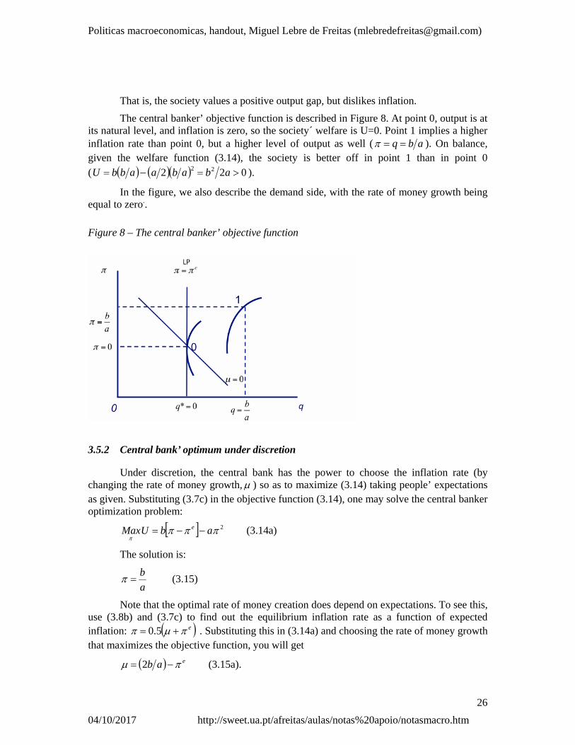
That is, the society values a positive output gap, but dislikes inflation.
The central banker’ objective function is described in Figure 8. At point 0, output is at its natural level, and inflation is zero, so the society´ welfare is U=0. Point 1 implies a higher inflation rate than point 0, but a higher level of output as well ( abq ). On balance, given the welfare function (3.14), the society is better off in point 1 than in point 0
( 022 22 ababaabbU ).
In the figure, we also describe the demand side, with the rate of money growth being equal to zero..
Figure 8 – The central banker’ objective function
3.5.2 Central bank’ optimum under discretion
Under discretion, the central bank has the power to choose the inflation rate (by changing the rate of money growth, ) so as to maximize (3.14) taking people’ expectations as given. Substituting (3.7c) in the objective function (3.14), one may solve the central banker optimization problem:
2
abUMax e (3.14a)
The solution is:
a
b (3.15)
Note that the optimal rate of money creation does depend on expectations. To see this, use (3.8b) and (3.7c) to find out the equilibrium inflation rate as a function of expected inflation: e 5.0 . Substituting this in (3.14a) and choosing the rate of money growth that maximizes the objective function, you will get
eab 2 (3.15a).
Politicas macroeconomicas, handout, Miguel Lebre de Freitas ([email protected])
27
04/10/2017 http://sweet.ua.pt/afreitas/aulas/notas%20apoio/notasmacro.htm
Thus, the optimal monetary expansion when 0e is ab2 , delivering
ab .
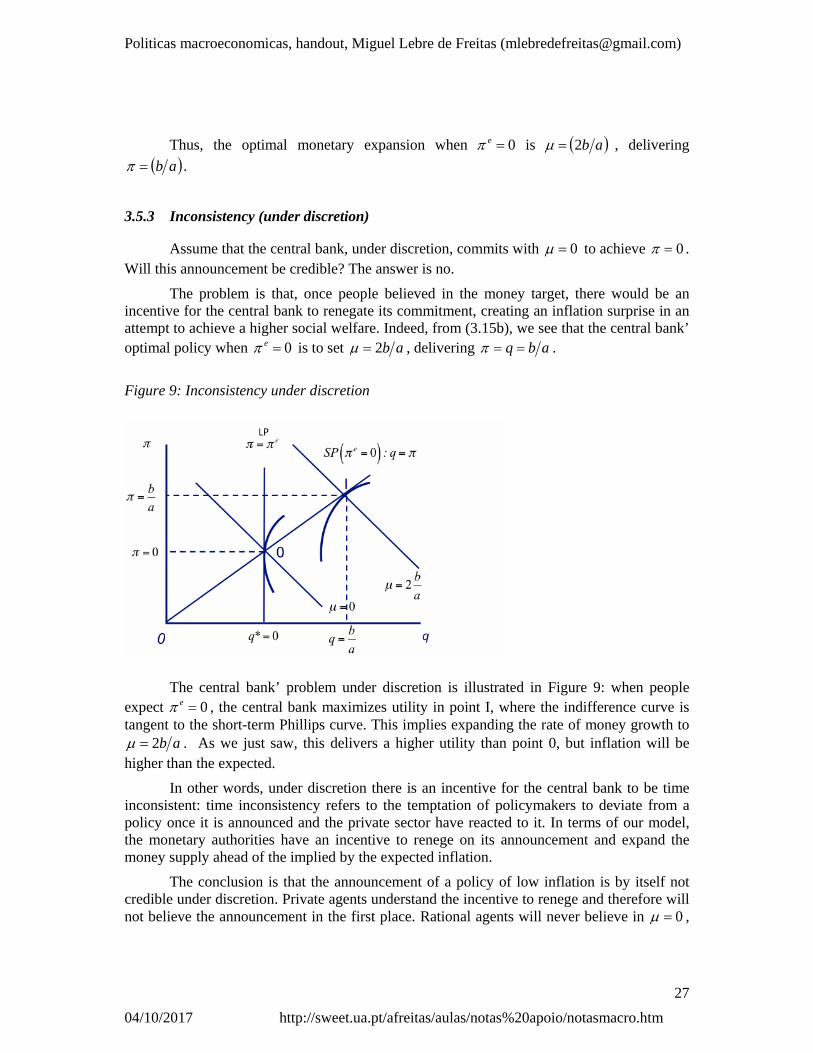
3.5.3 Inconsistency (under discretion)
Assume that the central bank, under discretion, commits with 0 to achieve 0 . Will this announcement be credible? The answer is no.
The problem is that, once people believed in the money target, there would be an incentive for the central bank to renegate its commitment, creating an inflation surprise in an attempt to achieve a higher social welfare. Indeed, from (3.15b), we see that the central bank’ optimal policy when 0e is to set ab2 , delivering abq .
Figure 9: Inconsistency under discretion
The central bank’ problem under discretion is illustrated in Figure 9: when people expect 0e , the central bank maximizes utility in point I, where the indifference curve is tangent to the short-term Phillips curve. This implies expanding the rate of money growth to
ab2 . As we just saw, this delivers a higher utility than point 0, but inflation will be higher than the expected.
In other words, under discretion there is an incentive for the central bank to be time inconsistent: time inconsistency refers to the temptation of policymakers to deviate from a policy once it is announced and the private sector have reacted to it. In terms of our model, the monetary authorities have an incentive to renege on its announcement and expand the money supply ahead of the implied by the expected inflation.
The conclusion is that the announcement of a policy of low inflation is by itself not credible under discretion. Private agents understand the incentive to renege and therefore will not believe the announcement in the first place. Rational agents will never believe in 0 ,

Politicas macroeconomicas, handout, Miguel Lebre de Freitas ([email protected])
28
04/10/2017 http://sweet.ua.pt/afreitas/aulas/notas%20apoio/notasmacro.htm
because they know that the central bank could be tempted to surprise them, setting ab2 once expectations are formed.
3.5.4 Consistency (under discretion)
Under rational expectations, the public is aware of the central banker’ preferences, and will form expectations accordingly. The consistent equilibrium under discretion is obtained when people formulate their expectations taking (3.15) into account. In this model, the only consistent expectation is:
a
be
In this equilibrium, the inflation rate is sufficiently high to deprive the central bank from any incentive to spring an inflation surprise. Under consistency, it is optimal for the central bank to exactly validate the public’ believes, setting ab .
Figure 10: Consistent equilibrium under discretion
The consistent equilibrium is described by point C in Figure 10. The problem with the consistent equilibrium, is that it delivers the same level of output as in point 0, but with higher inflation. The society pays the cost of inflation with no benefit at all. Note that the

Politicas macroeconomicas, handout, Miguel Lebre de Freitas ([email protected])
29
04/10/2017 http://sweet.ua.pt/afreitas/aulas/notas%20apoio/notasmacro.htm
utility level in point C is 022 abU , lower than in point 0. The consistent equilibrium is not efficient15.
3.5.5 Rules and other remedies
The surprising result of this model is that policymakers may better achieve their goals by having their discretionary power taken away from them. An obvious way the central bank can credibly commit with 0 is setting 0 as a rule. If the central bank abdicates from its discretionary power, adopting a legal rule from which it cannot deviate, then the resulting equilibrium will be superior. Once the central bank is constrained in its choices, citizens will not be exposed to the risk of “temptation”, enjoying a higher welfare than in the consistent equilibrium under discretion.
This is not, however, the only avenue. In practice, governments overcome this problem by choosing a central banker which personal tastes are more-anti-inflationary than those of the public at large, so that the central banker will lean against inflationary pressures. There are also experiences whereby the chairman of the central bank is offered a contract with payments that rewards low inflation.
3.5.6 The role of policy
How to minimize social losses when policy actions have to be taken frequently is a question that always concerned economists. Should policymakers act according to rules which dictate the choices to be made at any moment in time? Or should policymakers have instead the discretionary power to decide the best policy each moment in time, without being bounded by any constraint?
The case against activism had been already made by Milton Friedman. Friedman believed that market economies are inherently stable in the absence of unexpected fluctuations in the money supply. Even though monetary policy is a powerful tool, he argued, governments may lack the knowledge and the will to effectively stabilize the economy. Distrusting policymakers and the political process, Friedman defended that central banks
15 Extending this analysis to many periods, Barro and Gordon (1983) found out that a forward looking
policymaker will realize the value of building reputation. The reason is that after deviating from the target inflation, the policymaker will face a credibility loss and the economy will be driven to the bad equilibrium. Taking this into account, the policymaker will refrain from inflating. Still, the society will perceive that the central bank has incentives to cheat at any time, and that the incentives will be higher after reputations is built. Thus, in general, the society will expect a positive inflation. Still, the existence of reputation allows the consistent inflation rate under discretion to be lower than in the one period game [Barro, R. J. , Gordon, D., 1983. Rules, discretion and reputation in a model of monetary policy. Journal of monetary economics 12, 101-21].

Politicas macroeconomicas, handout, Miguel Lebre de Freitas ([email protected])
30
04/10/2017 http://sweet.ua.pt/afreitas/aulas/notas%20apoio/notasmacro.htm
should commit with steady money growth (hence, the label “monetarism”), rather than to follow discretionary policies.
It was however with the rational expectations revolution that the role of policy was seriously questioned. First, the monetary policy ineffectiveness proposition states that central banks may not be successful in expanding output. Second, under rational expectations the outcome of policy actions in uncertain, because we cannot be sure to what extent the policy is anticipated. Thus, an activist policy will have no predictable effect on output and cannot be relied on for stabilization purposes. Instead, it may create a lot of uncertainty about policy, translating into undesirable output fluctuations around the natural rate. Such an undesirable effect is exactly the opposite of what the activist stabilization policy is trying to achieve. Third, the time inconsistency argument states a policymaker entrusted with discretionary power may face a credibility problem. Incentives of policymakers to stick with the announced policy change once private agents adjust their expectations to the announced policy. Thus, economic performance may improve if private decision makers know for sure that the central bank will follow a rigid rule.
3.6 The new Keynesian response
The policy ineffectiveness proposition was challenged by a number of authors, who launched the New Keynesian School. The New Keynesian School is rooted on the Keynesian postulate that markets are imperfect and do not always clear. The NK school goes however beyond the Keynesian model, in trying to explain why prices and wages adjust slowly. The old Keynesian model had been discredited, because it was based on macroeconomic aggregates and ad-hoc assumptions, without taking into account individual optimization. The New Keynesian school overcame this criticism, coming up with new models, grounded on microeconomics and incorporating rational expectations. The appeal of the new school was trying to identify sources of frictions that prevent wages and prices from fully adjust to change in the price level, even when fully expected. The aim was to demonstrate that price stickiness is not incompatible with microeconomic foundations and rationality, and show how optimizing firms and workers make choices that may have adverse consequences to macroeconomics.
3.6.1 Staggered wages

Politicas macroeconomicas, handout, Miguel Lebre de Freitas ([email protected])
31
04/10/2017 http://sweet.ua.pt/afreitas/aulas/notas%20apoio/notasmacro.htm
The first wave of the new Keynesian school focused on labour contracts, to explain the sluggish adjustment of nominal wages16. Wages are set by multi-period contracts. Thus, even if new information becomes available making desirable a change in nominal wages, workers may find themselves locked into a wage agreement. Later, when the contract is renegotiated, both workers and firms are given the opportunity to incorporate the new information in the new contract. Meanwhile, however, they have to stick with what they agreed.
Another characteristic of wage revisions is that they are staggered over time: while some months are more popular than others for adjusting wage contracts, these adjustments are generally staggered throughout the year. Thus, when new information arises, instead of a sudden synchronized adjustment of wages - like in the neo-classical model - the model with staggered wages predicts a slow adjustment process, whereby a fraction of the existing contracts is revised each year, leapfrogging those that are still locked in their contract periods.
The central result of this theory is that wages don’t respond fully to changes in the expected price level. Hence, output will return slowly to its natural rate, even under rational expectations. Interesting enough, this recovers the Friedman’ claim that adjustment processes are long.
3.6.2 Anticipated changes do matter
To see how staggered wage contracts may change the conclusions of our model, let’s consider again the case with a monetary expansion from M=1 to M=4. This case is re-examined in Figure 11.
As before, the initial equilibrium is described by point 0, where M=1 and P=1. Then, the monetary authorities expand the money supply, driving the aggregate demand to 4=PQ. In the figure, three equilibria with rational expectations are considered:
Point 1 describes the case in which the monetary expansion is unexpected: irrespectively of how sticky wages are, when the move is not expected, there is no adjustment in the AS curve. The equilibrium following a monetary surprise is the same as in the case with flexible prices, either with adaptive or with rational expectations.
Point 1’ corresponds to the case in which the monetary shift is anticipated at t-1, and wages and prices are flexible. As we already saw, in this case there are no real effects and all money expansion is fully reflected in increasing prices. Since the money supply shifts from
1M to 4M , prices immediately adjust to P=4 and there are no real effects.
16 Phelps, E. S. (1968). "Money-Wage Dynamics and Labor Market Equilibrium". Journal of Political
Economy 76 (S4): 678–711. Fischer, S. (1977) Long-Term Contracts, Rational Expectations, and the Optimal Money Supply Rule Journal of Political Economy. Taylor, J. (1979), 'Staggered wage setting in a macro model'. American Economic Review, Papers and Proceedings 69 (2), pp. 108–13.

Politicas macroeconomicas, handout, Miguel Lebre de Freitas ([email protected])
32
04/10/2017 http://sweet.ua.pt/afreitas/aulas/notas%20apoio/notasmacro.htm
Point 1’’ describes the case in which the monetary shift is anticipated at time t-1, but some fraction of the labour contracts is locked into wage agreements that were set previous to the announcement. Even though all workers are now aware that money will expand from M=1 to M=4, some will face a real wage loss, because they are not allowed to reset their contracts. Hence, the short term aggregate supply adjusts only half-way, and output expands ahead of its natural level, even if the monetary expansion is announced at time 0. In the example in Figure 11, the “half-way” supply curve is described assuming that 314eP , implying a short term equilibrium at 314Q and 324P (see Box 3.4 for a more formal explanation).
Figure 11: Monetary shock under rational expectations and staggered wage contracts
Thus, just like in the new-classical model, an unanticipated monetary shift has a larger effect on output than an anticipated monetary change. The novelty with staggered wage contracts is that the ineffectiveness proposition does not hold: an anticipated monetary disturbance produces real effects, because some fraction of the agents in the economy cannot reset their wages17. This theory is grounded in empirical evidence, that anticipated monetary changes do have real effects18 .
17 Also note that, in case the policy is anticipated, the economy moves from point 0 to point 1’’ at t=1
and then to point 1’ in t=2. In contrast, when the change in money is not anticipated, all agents will be frustrated at time t=1, and final equilibrium in point 1’ will be reached at t=3, only.
18 Mishkin, Frederic S. 198a. ''Does Anticipated Monetary Policy Matter? An Econometric Investigation.'' Journal of Political Economy 90 (February 1982): 21– 51.

Politicas macroeconomicas, handout, Miguel Lebre de Freitas ([email protected])
33
04/10/2017 http://sweet.ua.pt/afreitas/aulas/notas%20apoio/notasmacro.htm
This finding has two implications: first, monetary policy can now be used to offset shocks and stabilize output. Second, since the adjustment to full employment is faster and less costly when the policy is anticipated, monetary authorities should be transparent in their intentions.
Box 3.4. The staggered wages model
To see how the model works with staggered wages, we have to amend it from the very beginning. In particular, let’s start out with equation (3.3), that describes the supply function, and (3.4) that describes the relationship between nominal wages and expected prices. As for the supply function, we already presented in the log form, (3.3a) – See Box 3.1. In respect to the equation (3.4), we now adapt the theory.
Suppose that in this economy wages are locked in two-period contracts. In each contract, workers and employees set the wage rates for two consecutive years, with the possibility of these wages being different each year. Thus, at time t-2 wages for periods t-1 and t are negotiated. Further assume that in this economy, half of the contracts are negotiated each year. This means that half of current wages were set in period t-2 and the other half were set in period t-1. In such framework, one needs to replace equation (3.4) by:
pEpEw 122
1ln (3.4b)
Replacing this in (3.3a), we get:
pEpEpqq 21
*
2
1
2
11
(3.6c)
where *q is the same as before. Now using (3.8a) to eliminate q, we get our new equilibrium solution, as a function of expectations:
*212
11 qmpEpEp (3.9b)
pEpEmqq 21* 1 (3.10b)
Equation (3.9b) describes the price formation in a world where labour contracts last for two years and half of labour contracts are negotiated each year. Note that in case
mEmE 21 equations (3.9b) and (3.10b) deliver (3.9a) and (3.10a)
If expectations are rational, they have to be consistent with this rule. Thus, the expectations formed at t-2 shall be:
*2222 2
11 qmEpEpEpE
Which solves for *
22 qmEpE (3.12b)
The expectation formed at t-1 is trickier, because it has to take into account that the earlier expectations are already materialized in labour contracts.

Politicas macroeconomicas, handout, Miguel Lebre de Freitas ([email protected])
34
04/10/2017 http://sweet.ua.pt/afreitas/aulas/notas%20apoio/notasmacro.htm
Replacing (3.12b) in (3.9b) we get the relevant equation describing the behaviour of prices for those agents negotiating at t-1:
**212
11 qmqmEpEp
Note that expectations at t-2 were already formed and cannot be changed. The expectations at t-1 are:
*1
*211 2
11 qmEqmEpEpE
Which solves for
*211 1
112
qmEmEpE
(3.12c)
Again, in case mEmE 21 equations (3.12b) and (3.12c) deliver (3.12a).
Finally, let’s replace (3.12b) and (3.12c) in (3.10b), to obtain:
mEmEmqq 21*
1
1
11
(3.13b)
Or, rearranging:
mEmEmEmqq 211
*
1
11
This equation differs from (3.13) in that a fraction 11 of unexpected changes in money between t-2 and t-1 pass into output at time t, even though workers at time t-1 were already aware of that change. This reflects the fact that not all wages are negotiated at t-1. Workers setting wages at t-1 have the opportunity to respond to changes in money supply that became known at t-1. But workers who have set their wages in period t-2 have to wait one period to adjust their labour contracts.
3.6.3 Policy implications
With the rational expectations revolution, economists became less confident in the success of activist stabilization policies than they were before. Since expectations change with the policy, the success of a particular policy will depend critically on the public's expectations about that policy. If the policy becomes unpredictable, the game between policymakers and the public may be highly destabilizing. To eliminate undesirable fluctuations of output around its natural rate, the monetary authorities should thus generate as few policy surprises as possible. Central bankers should abandon discretionary policy and follow clear and transparent rules. This includes a strong commitment with low inflation.
The New Keynesian School challenged the view that expected monetary actions only deliver price effects. The contention is that monetary policy can influence output, even under rational expectations. This recovers the stabilization role of monetary policy. In light of the

Politicas macroeconomicas, handout, Miguel Lebre de Freitas ([email protected])
35
04/10/2017 http://sweet.ua.pt/afreitas/aulas/notas%20apoio/notasmacro.htm
New-Keynesian model, monetary policy shall not be used to achieve short-term gains, but it can be used to offset unexpected shocks and stabilize output.
The finding that anticipated changes in money produce real effects has implications for the design of a disinflation programme. If prices were flexible, the central banks could respond to inflation surges with shock therapy, as this would enhance credibility, allowing agents to align faster their expectations with the policymaker intentions, and delivering faster price adjustment and lower output costs (“cold turkey” argument).
When however agents are locked in multi-year contracts, prices cannot adjust swiftly. Thus, there will be real costs even when the policy is credible. Therefore, the best policy will be a gradual adjustment, so as to give agents time to revise their contracts. Such policy should be smooth and communicated as much in advance as possible, so as to avoid agents to be taken by surprise: disinflation costs are unavoidable, but they are lower when the policy is credible. Of course gradual policies are inherently less credible than shock therapies. But the central bank may be able to overcome this by building up reputation. The new wisdom is that central banks may help stabilize the economy, but following clear rules, being transparent regarding their forecasts and committed with their intentions.
3.7 Further reading
Barbosa, A. P., 2011. Macroeconomia. Fundação Calouste Gulbenkian. Chapter 7.2.
Driscoll, John, 20013. Lectures in Macroeconomics. Brown University. Chapters 2.3, 2.4, 3.2, 3.3.
Gordon, R., 2012, Macroeconomics, 12th edition: Chapter 17.
Montiel, P., 2003. Macroeconomic in Emerging Markets. Cambridge University Press. Cambridge. Chapter 9.
Romer, D., 2001. Advanced Macroeconomics. McGraw-Hill. Chapter 10.4.
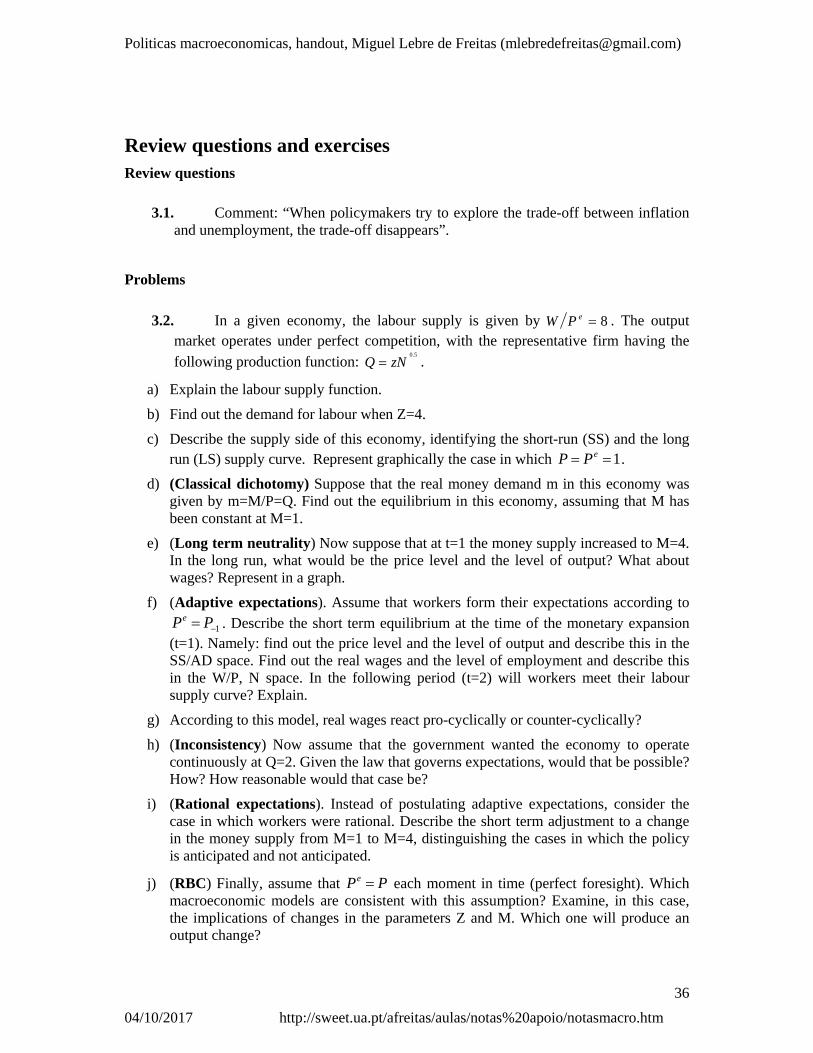
Politicas macroeconomicas, handout, Miguel Lebre de Freitas ([email protected])
36
04/10/2017 http://sweet.ua.pt/afreitas/aulas/notas%20apoio/notasmacro.htm
Review questions and exercises Review questions
3.1. Comment: “When policymakers try to explore the trade-off between inflation and unemployment, the trade-off disappears”.
Problems
3.2. In a given economy, the labour supply is given by 8ePW . The output market operates under perfect competition, with the representative firm having the
following production function: 5.0
zNQ .
a) Explain the labour supply function.
b) Find out the demand for labour when Z=4.
c) Describe the supply side of this economy, identifying the short-run (SS) and the long run (LS) supply curve. Represent graphically the case in which 1 ePP .
d) (Classical dichotomy) Suppose that the real money demand m in this economy was given by m=M/P=Q. Find out the equilibrium in this economy, assuming that M has been constant at M=1.
e) (Long term neutrality) Now suppose that at t=1 the money supply increased to M=4. In the long run, what would be the price level and the level of output? What about wages? Represent in a graph.
f) (Adaptive expectations). Assume that workers form their expectations according to
1 PPe . Describe the short term equilibrium at the time of the monetary expansion (t=1). Namely: find out the price level and the level of output and describe this in the SS/AD space. Find out the real wages and the level of employment and describe this in the W/P, N space. In the following period (t=2) will workers meet their labour supply curve? Explain.
g) According to this model, real wages react pro-cyclically or counter-cyclically?
h) (Inconsistency) Now assume that the government wanted the economy to operate continuously at Q=2. Given the law that governs expectations, would that be possible? How? How reasonable would that case be?
i) (Rational expectations). Instead of postulating adaptive expectations, consider the case in which workers were rational. Describe the short term adjustment to a change in the money supply from M=1 to M=4, distinguishing the cases in which the policy is anticipated and not anticipated.
j) (RBC) Finally, assume that PPe each moment in time (perfect foresight). Which macroeconomic models are consistent with this assumption? Examine, in this case, the implications of changes in the parameters Z and M. Which one will produce an output change?
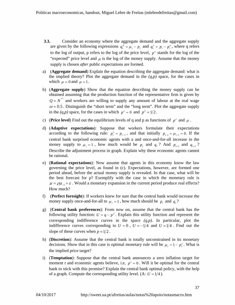
Politicas macroeconomicas, handout, Miguel Lebre de Freitas ([email protected])
37
04/10/2017 http://sweet.ua.pt/afreitas/aulas/notas%20apoio/notasmacro.htm
3.3. Consider an economy where the aggregate demand and the aggregate supply are given by the following expressions tt
dt pq and e
ttst ppq , where q refers
to the log of output, p refers to the log of the price level, ep stands for the log of the “expected” price level and is the log of the money supply. Assume that the money supply is chosen after public expectations are formed.
a) (Aggregate demand) Explain the equation describing the aggregate demand: what is the implied theory? Plot the aggregate demand in the (q,p) space, for the cases in which 0 and 1 .
b) (Aggregate supply) Show that the equation describing the money supply can be obtained assuming that the production function of the representative firm is given by
5.0
NQ and workers are willing to supply any amount of labour at the real wage 5.0 . Distinguish the “short term” and the “long term”. Plot the aggregate supply
in the (q,p) space, for the cases in which 0ep and 21ep .
c) (Price level) Find out the equilibrium levels of q and p as functions of ep and .
d) (Adaptive expectations): Suppose that workers formulate their expectations according to the following rule: 1 t
et pp , and that initially .011 ttp If the
central bank surprised economic agents with a and once-and-for-all increase in the money supply to 1t , how much would be tp and tq ? And 1tp and 1tq ?
Describe the adjustment process in graph. Explain why these economic agents cannot be rational.
e) (Rational expectations): Now assume that agents in this economy know the law governing the price level, as found in (c). Expectations, however, are formed one period ahead, before the actual money supply is revealed. In that case, what will be the best forecast for p? Exemplify with the case in which the monetary rule is
1 . Would a monetary expansion in the current period produce real effects? How much?
f) (Perfect foresight): If workers knew for sure that the central bank would increase the money supply once-and-for-all to 1t , how much should be tp and tq ?
g) (Central bank preferences): From now on, assume that the central bank has the following utility function: 2pqU . Explain this utility function and represent the corresponding indifference curves in the space (q,p). In particular, plot the indifference curves corresponding to 0U , 41U and 41U . Find out the slope of these curves when 21p .
h) (Discretion): Assume that the central bank is totally unconstrained in its monetary decisions. Show that in this case is optimal monetary rule will be e
tt p 1 . What is
the implied price target?
i) (Temptation): Suppose that the central bank announces a zero inflation target for moment t and economic agents believe, i.e, 0ep . Will it be optimal for the central bank to stick with this promise? Explain the central bank optimal policy, with the help of a graph. Compute the corresponding utility level. (A: 41U ).

Politicas macroeconomicas, handout, Miguel Lebre de Freitas ([email protected])
38
04/10/2017 http://sweet.ua.pt/afreitas/aulas/notas%20apoio/notasmacro.htm
j) (Inconsistency): Explain why the above equilibrium is inconsistent. Could this central bank credibly commit with the zero-inflation target under discretion?
k) (Consistency): If the public was aware of the central bank preferences, how much would be
ep ? In that case, what would be the central bank optimal choice for ? Explain why such equilibrium would be consistent. Compute the central bank utility level in this case. (A: 41U ).
l) (Rule) Finally, assume that the central bank is forced to follow the rule 0 . Assuming that this rule is fully enforced by law and that the public is aware of this, what would be the equilibrium? Compare the central bank utility level in this case to the case with discretion. (A: 0U ).
m) What does this exercise suggest regarding the optimal institutional design of a central bank?
3.4. Consider an economy where the aggregate demand and the aggregate supply are given, respectively, by M=PY and ePPY . In this economy, M has been constant at M=1
a) (Theory) Explain the two equations.
b) (Anticipated change) Suppose that, at t=1, the money supply changed from M=1 to M=9. If the policy was announced and it was credible, how much should output and prices be?
c) (Adaptive expectations). Assume that workers formed their expectations according to
1 PPe . Assuming that in the period before P=1, describe the short term equilibrium at the time of the monetary expansion (t=1), as well as the subsequent adjustment of the economy to the long run.
d) (Discretion): Suppose that the central bank’ preferences were given by 2114 PYU and well known by the public. Could the central bank under
discretion credibly commit with P=1? And with P=2?
3.5. Consider an economy where the mandate of the central bank includes ensuring price stability and an adequate level of employment in the economy. In this economy, agents are rational and perceive the central bank objective function to take the following form: 205.05 pppU e , where p refers to inflation and ep refers to expected inflation.
a) Explain the central bank objective function.
b) Suppose the central bank announced the inflation rate to be 5%. Will this announcement be credible?
c) Sticking to the case with discretion, which inflation target would be fully credible? Explain, with the help of a graph.

Politicas macroeconomicas, handout, Miguel Lebre de Freitas ([email protected])
39
04/10/2017 http://sweet.ua.pt/afreitas/aulas/notas%20apoio/notasmacro.htm
d) Suppose the parliament in this country was considering restricting the mandate of the central bank to pursue the objective of price stability only (inflation 5%). Would such change be welfare improving in this context?
e) Explain the policy implications of this model.
3.6. (Staggered wage contracts). Consider an economy where the supply function is tt
st wpq , and the aggregate demand is given by tt
dt pq , where q refers to
the log of output, to the log of the money supply, w to the log of wages, and p to the log of the price level.
a) (One-period ahead wages): Assume that workers set their wages one period in advance, implying ttt pEw 1 . Find out the equilibrium expressions for prices and
output as functions of expected prices and of actual money supply. Show that in this case, only unanticipated changes in money supply produce real effects, and only for one period.
b) (Two-period ahead wages): Sticking with the assumption of rational expectations, assume now that wages in this economy were set two-periods in advance, with half of the economy setting wages in even years and the other half in odd years, implying
ttttt pEpEw 215.0 . (b1) find out the equilibrium price level as a function of
p2 , p1 , and m. (b2) Find out the best forecast for p2 , as a function of m2 .
(b3) Find out the best forecast for p1 , as a function of m2 and m1 . (b4) Using
(b1), (b2), (b3), find out the expression for q as a function of m, m2 and m1 . (b5)
Assume now that the money supply followed a random walk, that is, 1 .
Prove that 13121 q . (b6) Discuss this result.