31301578 quantitative techniques 1

8/2/2019 31301578 Quantitative Techniques 1

http://slidepdf.com/reader/full/31301578-quantitative-techniques-1 1/37

Quantitative Techniques

inManagement

Dr. Gayatri V Singh, PhD,

AMITY University,

INDIA

http://images.google.co.in/imgres?imgurl=http://pages.cms.k12.nc.us/pictures/stephengilbert/goodnormalcurve.png&imgrefurl=http://pages.cms.k12.nc.us/stephengilbert/discretelesson.html&usg=__xJWc8Earg2pUQ1nEQwG1EMpdE7Q=&h=435&w=683&sz=58&hl=en&start=5&itbs=1&tbnid=-YhV2zghVufDlM:&tbnh=89&tbnw=139&prev=/images?q=what+is+statistics&hl=en&gbv=2&tbs=isch:1

http://images.google.co.in/imgres?imgurl=http://www.unesco.org/webworld/projects/image/statistic5.gif&imgrefurl=http://www.unesco.org/webworld/projects/statistics.html&usg=__xrnmFOV8LnXKN1bbUj2VTYyPZwE=&h=480&w=448&sz=34&hl=en&start=8&itbs=1&tbnid=NRwtQT3HbORIfM:&tbnh=129&tbnw=120&prev=/images?q=statistic&hl=en&gbv=2&tbs=isch:1

http://images.google.co.in/imgres?imgurl=http://dragonartz.files.wordpress.com/2008/12/_graphics-statistics-graph-preview3-by-dragonart.png?w=495&h=495&imgrefurl=http://dragonartz.wordpress.com/2008/12/05/&usg=__Ip1xvZQJSUflNbfQhzDOtwm5Ivo=&h=495&w=495&sz=68&hl=en&start=7&itbs=1&tbnid=3Pv_jFzGZ9IZYM:&tbnh=130&tbnw=130&prev=/images?q=statistics&hl=en&sa=G&gbv=2&tbs=isch:1



Today’s Highlights

• Introduction

• Application in Business and Management

• Classification of Data

• Graphical Presentation of Data

• Mean and Variance

•

Correlation Analysis• Regression Analysis



What is Statistics?

It is the science of collecting, organizing,presenting, analyzing, and interpreting data(quantitative or qualitative) for the purpose of assisting in making a more effective decision.

WHO USES STATISTICS?

Statistical techniques are used extensively bymarketing, accounting, quality control,

consumers, professional sports people, hospitaladministrators, educators, politicians,physicians, etc.



Applications

• For empirical inquiry

• Financial Decisions

• How is the economy doing?

• The impact of technology at work

• Compensation survey• Perfomance management

• Employee Satisfaction Survey

•

Training feedback evaluation• Human Resource Accounting

• HR Budgeting



Statistical Methods

Statistics

Descriptive Univariate

Analysis Multivariate



Statistical Methods Contd…

Descriptive

• Frequency Distribution

•Measurement of Central Tendency

•Measurement of Dispersion

•Graphical Presentationof Data

Analysis/Inferential

• Correlation andRegression Analysis

• Estimation Theory

•Hypothesis Testing

•Decision Theory•Operation Research



Data Classification

Data

Quantitativeor Numerical

Discrete Continuous

Qualitativeor Attribute

Nominal Ordinal

Number of students Temperature,Time taken for exam

Gender EducationRank of a performanc



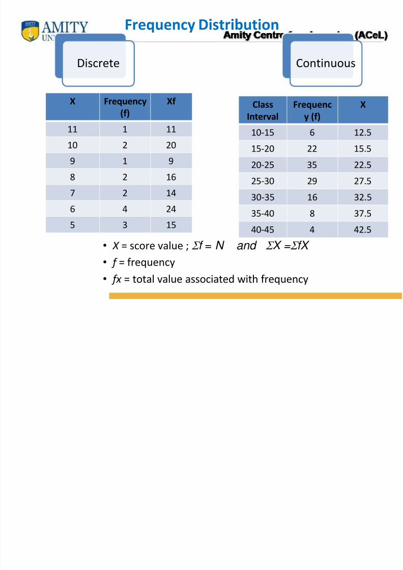
Frequency Distribution

Discrete Continuous

• X = score value ; f = N and X = fX

• f = frequency

•fx = total value associated with frequency

Class

Interval

Frequenc

y (f)

X

10-15 6 12.5

15-20 22 15.5

20-25 35 22.5

25-30 29 27.5

30-35 16 32.5

35-40 8 37.5

40-45 4 42.5

X Frequency

(f)

Xf

11 1 11

10 2 20

9 1 9

8 2 16

7 2 14

6 4 245 3 15



Graphs

Data

Qualitative

Or Numerical

Histogram

Frequency Polygon

Box Plot

Quantitative

Or Categorical

Bar Chart

Pie Chart



Histogram

A histogram is a bar graph that shows the frequency of data within

equal intervals. There is no space between the bars in a histogram



What is the most common age group for musicians?



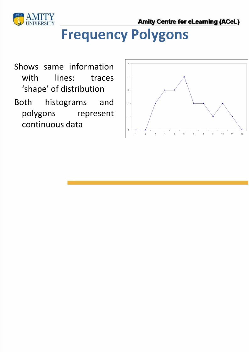
Frequency Polygons

Shows same information

with lines: traces

‘shape’ of distribution

Both histograms and

polygons represent

continuous data



A graph that uses a number line to show thedistribution of a set of data.

Second quartile: The median of the set of a data.Lower quartile: The median of the lower half of aset of data.Upper quartile: The median of the upper half ofthe set of data.Inter-quartile range: The difference between thelower and upper quartiles.

Box Plot



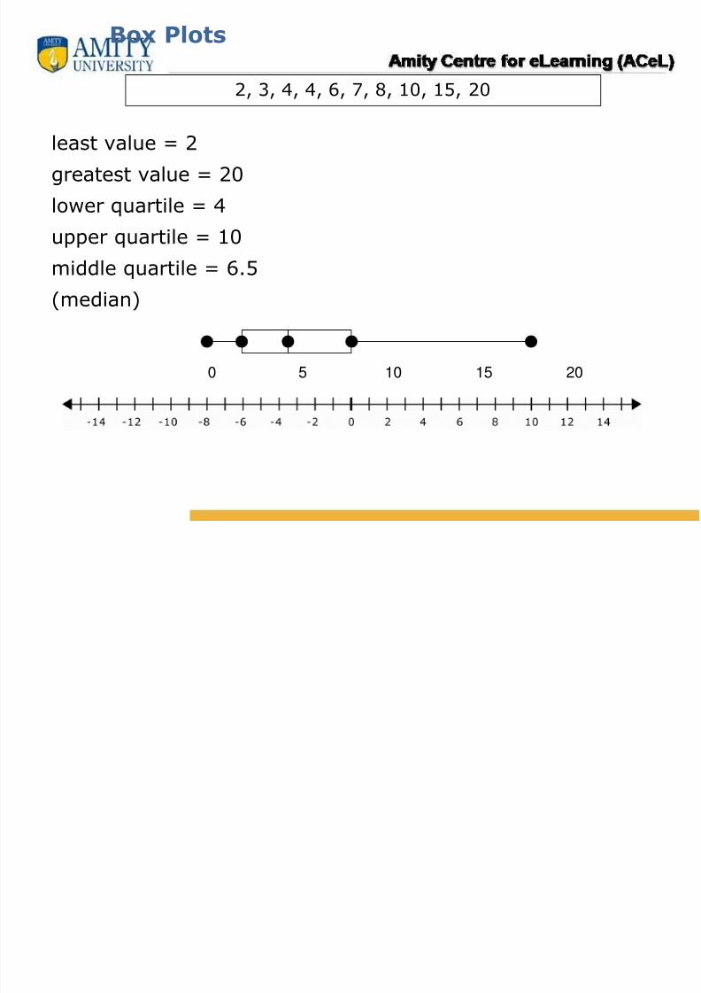
Box Plots

2, 3, 4, 4, 6, 7, 8, 10, 15, 20

least value = 2

greatest value = 20

lower quartile = 4

upper quartile = 10middle quartile = 6.5

(median)

0 5 10 15 20



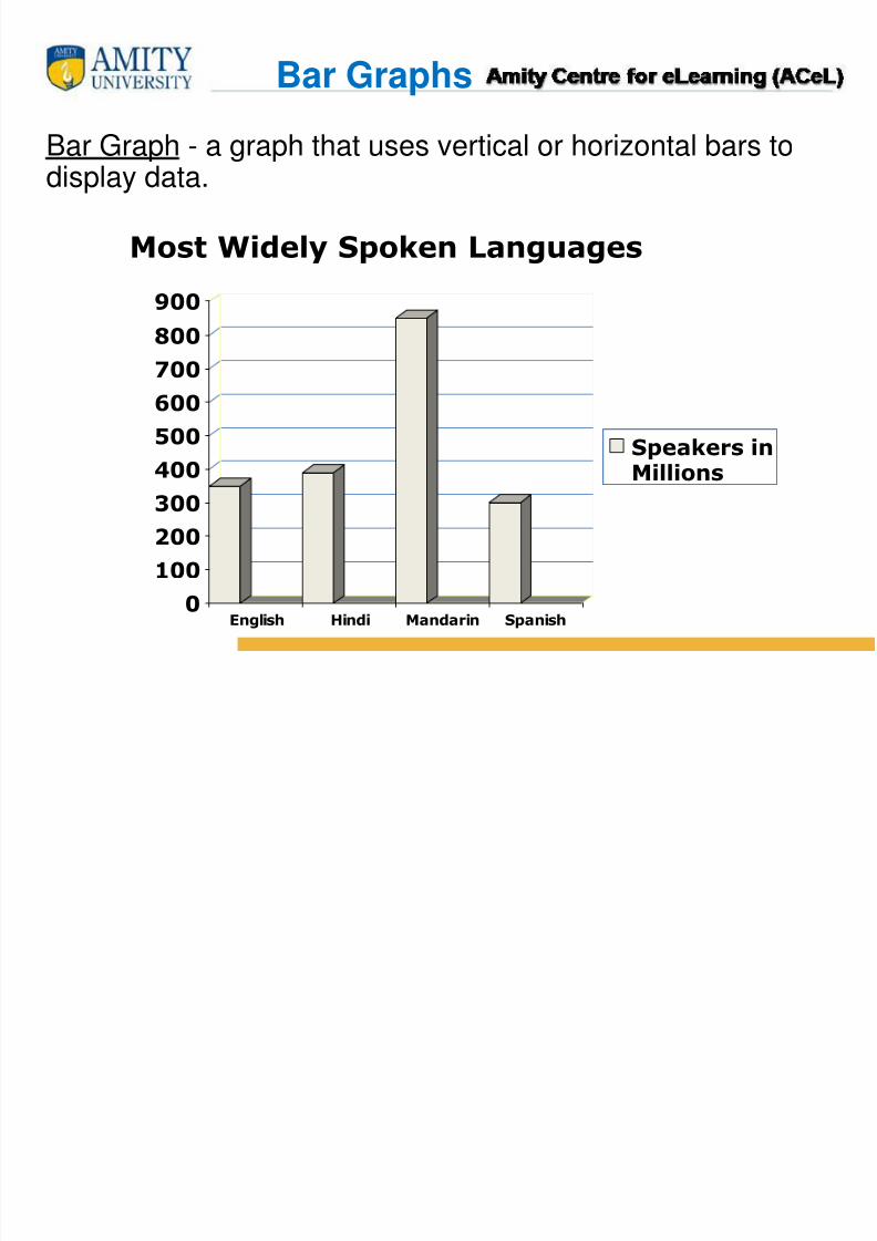
Bar Graphs

Bar Graph - a graph that uses vertical or horizontal bars todisplay data.

0

100

200

300

400

500

600

700

800900

English Hindi Mandarin Spanish

Speakers inMillions

Most Widely Spoken Languages



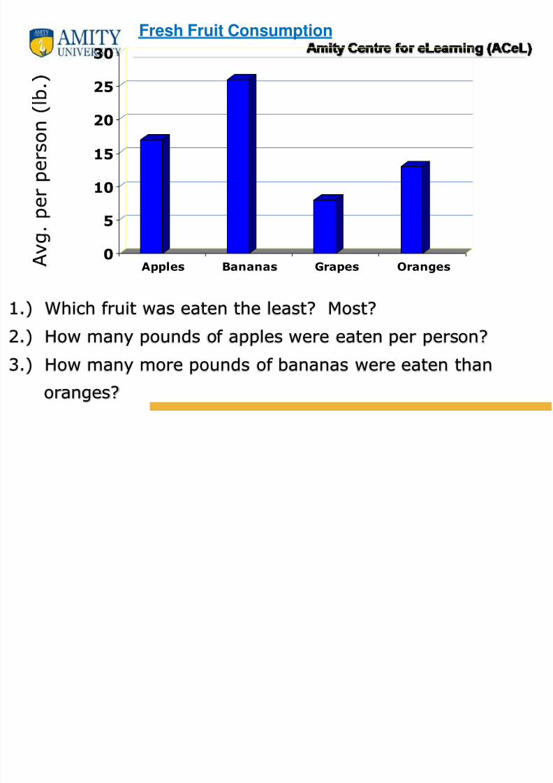
Fresh Fruit Consumption

0

5

10

15

20

25

30

Apples Bananas Grapes Oranges

1.) Which fruit was eaten the least? Most?

2.) How many pounds of apples were eaten per person?

3.) How many more pounds of bananas were eaten than

oranges?



Pie Chart

A pie chart (or a circlegraph) is circular chartdivided into sectors,illustrating proportion. In apie chart, the arc length ofeach sector (and

consequently its centralangle and area), isproportional to the quantityit represents.



Central Tendency

Mean, Median, Mode are measures of

central tendency. We can use them

to describe a set of data.



Mean: (Average)The sum of a set of numbers divided by the total

number of the set. To find the mean of the data set :

2, 1, 8, 0, 2, 4, 3, 4

Central Tendencies



Median: (Middle Value)

The number in the middle of a set of numbers that are

arranged in order from least to greatest.

To find the median of the data set : 2, 1, 8, 0, 2, 4, 3, 4



Mode: (Most frequent value)

The number that occurs most often in a set of numbers. There

can be 1 mode, more than 1 mode, or no mode.

To find the mode of the data set : 2, 1, 8, 0, 2, 4, 3, 4



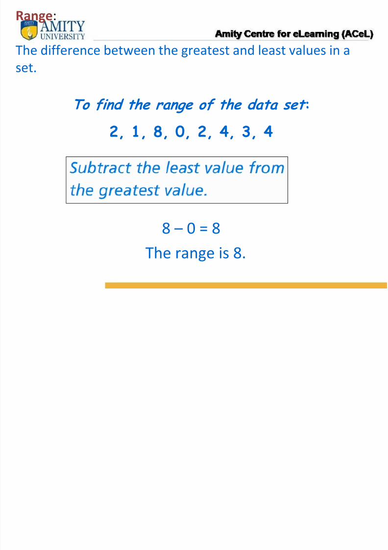
Range:

The difference between the greatest and least values in a

set.

To find the range of the data set : 2, 1, 8, 0, 2, 4, 3, 4

8 – 0 = 8

The range is 8.



Central Tendencies

Find the mean, median, mode and range of these numbers.

18, 21, 8, 12, 26

8, 12, 18, 21, 26

Mean = 8 + 12 + 18 + 21 + 26 = 85 = 17

5 5

Median = 8, 12, 18, 21, 26

Mode = NO MODE Range = 26 - 8 = 18



Central Tendencies

Find the mean, median, mode and range of these numbers.

80, 60, 76, 60, 90, 80, 70, 60

60, 60, 60, 70, 76, 80, 80, 90

Mean = 576 = 72

8

Median = 60, 60, 60, 70, 76, 80, 80, 90

Mode = 60 Range = 90 - 60 = 30

76 + 70 = 73

2



Measurement of Variability

• A certain amount of variability will naturallyoccur when a control is tested repeatedly.

•

Variability is affected by operator technique,environmental conditions, and theperformance characteristics of the assaymethod.

• The goal is to differentiate betweenvariability due to chance from that due toerror.



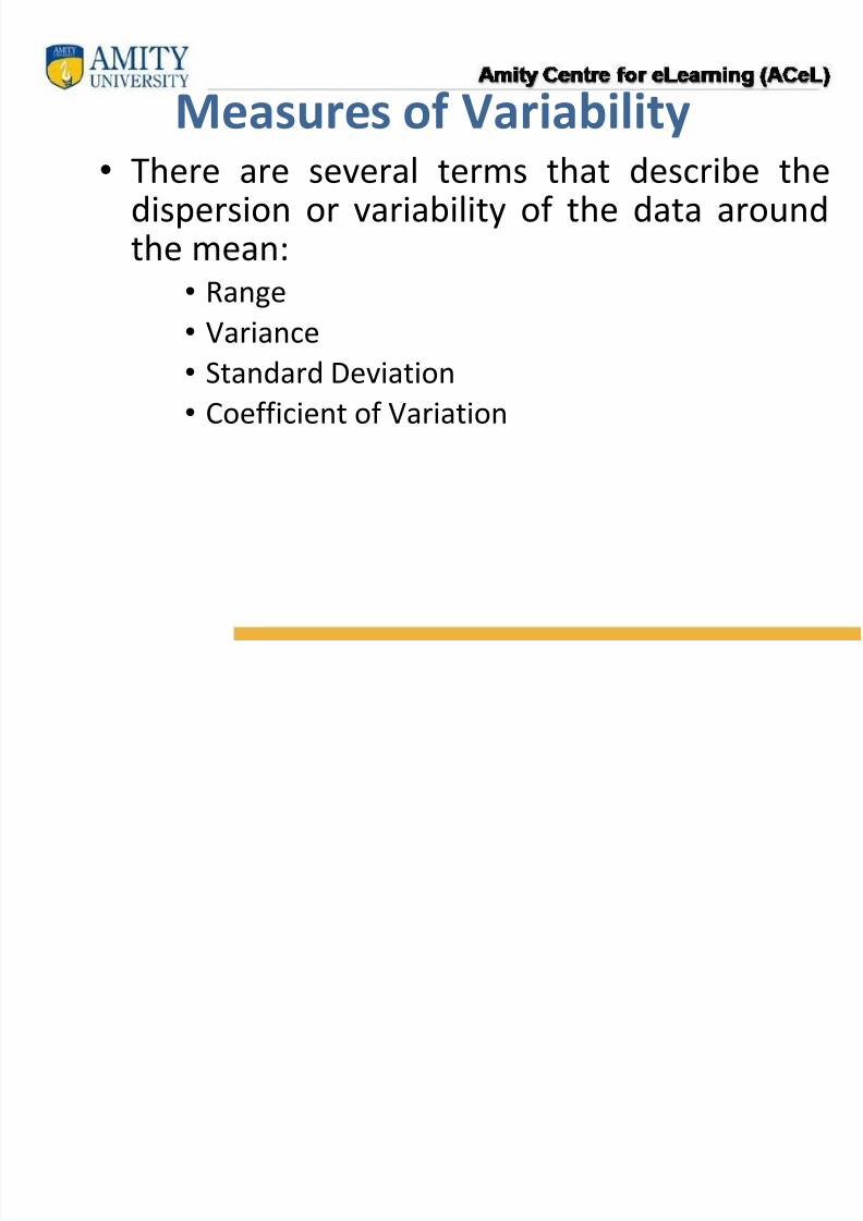
Measures of Variability• There are several terms that describe the

dispersion or variability of the data aroundthe mean:

•

Range• Variance

• Standard Deviation

• Coefficient of Variation



Calculation of Variance• Variance is the measure of variability about

the mean.

• It is calculated as the average squared

deviation from the mean. – the sum of the deviations from the mean,

squared, divided by the number of observations(corrected for degrees of freedom)



Correlation Analysis• the degree to which two variables are associated

• strength of the relationship (correlation)between two variables

• may be either positive or negative.• Its magnitude depends on the units of

measurement.

• Assumes the data are from a bivariate normalpopulation.

• Does not necessarily imply causation



Correlation Analysis

Data

Qualitative

Or Numerical

Karl PearsonCorrelationCoefficient

Quantitative

Or Categorical

Spearman’s

Rank Correlation



Correlation

• The value of r can range between -1 and +1.

• If r = 0, then there is no correlationbetween the two variables.

• If r = 1 (or -1), then there is a perfectpositive (or negative) relationship between

the two variables.



y1

y 2

-2 -1 0 1 2 3

- 2

- 1

0

1

2

3

y1

y 2

-2 -1 0 1 2 3

- 3

- 2

- 1

0

1

2

y1

y 2

-2 -1 0 1 2 3

- 4

- 3

- 2

- 1

0

1

2

r = + 1 r = - 1 r = 0

Scatter Plot



Calculation

CorrelationCoefficient

KarlPearson

Spearman

y x

xy

n y x xyr

/

n x x x / 22

n y y y /

22

)1(

61

2

2

nn

d

“d” is the difference between ranksof two variables



Regression analysis includes any techniques for modeling and analyzing

several variables, when the focus is on the relationship between a

dependent variable and one or more independent variables.

More specifically, regression analysis helps us understand how thetypical value of the dependent variable changes when any one of the

independent variables is varied, while the other independent variables

are held fixed.

Most commonly, regression analysis estimates the conditional

expectation of the dependent variable given the independent variables— that is, the average value of the dependent variable when the

independent variables are held fixed.

Regression Analysis

R i A l i



Regression Analysis

Purpose –

To determine the regression equation. It is used to predict

the value of one variable (Y , called the dependent

variable) based on another variable ( X , called the

independent variable). Procedure:

•Select a sample from the population, and list the paired data

( X , Y ) for each observation.

•Draw a scatter diagram to give a visual portrayal of therelationship.

•Determine the regression equation Y = a + bX .



Regression Analysis

x

y xy yx r b

y

x xy xy r b

xb ya yx

•Y is the average predicted value of Y for any X .

•a is the Y -intercept, or the estimated Y value when X = 0.

•b is called the slope of the line. It is the average change in Y for eachchange of one unit in X .

•The least squares principle is used to obtain a and b and are given by:



Example

• Develop a regression equation for the

information given in the EXAMPLE that can

be used to estimate the selling price based on

the number of pages.

• b = 0.01714, a = 16.00175.

• Y = 16.00175 + 0.01714X .

• What is the estimated selling price of a 650-

page book?

• Y = 16.00175 + 0.01714(650) = $27.14.



Thank you

You may send in your queries at

[email protected]

31301578 quantitative techniques 1

Documents