32. computationally manageable combinatorial - iiia - csic
TRANSCRIPT


MONOGRAFIES DE L’INSTITUT D’INVESTIGACIOEN INTEL·LIGENCIA ARTIFICIAL
Number XXXII
Institut d’Investigacioen Intel·ligencia Artificial
Consell Superiord’Investigacions Cientıfiques


Computationally Manageable Combinatorial
Auctions for Supply Chain Automation
Andrea Giovannucci
Foreword by Juan Antonio Rodriguez-Aguilar and Jesus Cerquides
2008 Consell Superior d’Investigacions CientıfiquesInstitut d’Investigacio en Intel·ligencia Artificial
Bellaterra, Catalonia, Spain.

Series EditorInstitut d’Investigacio en Intel·ligencia ArtificialConsell Superior d’Investigacions Cientıfiques
Foreword by Juan Antonio Rodriguez-Aguilara and Jesus Cerquidesb
a Institut d’Investigacio en Intel·ligencia ArtificialConsell Superior d’Investigacions Cientıfiques
b Departament de Matematica Aplicada y AnalisiUniversitat de Barcelona
Volume AuthorAndrea GiovannucciInstitut d’Investigacio en Intel·ligencia ArtificialConsell Superior d’Investigacions Cientıfiques
Institut d’Investigacioen Intel·ligencia Artificial
Consell Superiord’Investigacions Cientıfiques
c© 2008 by Andrea GiovannucciNIPO:653-08-087-XISBN:978-84-00-08666-4Dip. Legal: B-30348-2008
All rights reserved. No part of this book may be reproduced inany form or by any elec-tronic or mechanical means (including photocopying, recording, or information storageand retrieval) without permission in writing from the publisher.Ordering Information: Text orders should be addressed to the Library of the IIIA,Institut d’Investigacio en Intel·ligencia Artificial, Campus de la Universitat Autonomade Barcelona, 08193 Bellaterra, Barcelona, Spain.

I dedicate this piece of life to my father Alberto, mymother Carla, and my brother Marco.


Contents
Foreword xix
Abstract xxi
Acknowledgements xxiii
1 Introduction 11.1 A hypothesis for the future: Wikinomics . . . . . . . . . . . . . .. . . 11.2 With the feet in the air & the head on the ground . . . . . . . . . .. . . 31.3 Supply Chain and Supply Chain Management . . . . . . . . . . . . .. 61.4 The Problem . . . . . . . . . . . . . . . . . . . . . . . . . . . . . . . . 7
1.4.1 Optimising make-or-buy decisions . . . . . . . . . . . . . . . .71.4.2 Optimising make-or-buy-or-collaborate decisions .. . . . . . . 13
1.5 Contributions . . . . . . . . . . . . . . . . . . . . . . . . . . . . . . . 171.6 Dissertation Outline . . . . . . . . . . . . . . . . . . . . . . . . . . . . 20
2 Mathematical Background 232.1 Linear and Integer Programming . . . . . . . . . . . . . . . . . . . . .23
2.1.1 Linear Programming . . . . . . . . . . . . . . . . . . . . . . . 232.1.2 Integer Programming . . . . . . . . . . . . . . . . . . . . . . . 24
2.2 Multi-sets . . . . . . . . . . . . . . . . . . . . . . . . . . . . . . . . . 262.2.1 Operations on Multisets . . . . . . . . . . . . . . . . . . . . . 27
2.3 Petri Nets . . . . . . . . . . . . . . . . . . . . . . . . . . . . . . . . . 272.3.1 Reachability . . . . . . . . . . . . . . . . . . . . . . . . . . . 312.3.2 The state equation . . . . . . . . . . . . . . . . . . . . . . . . 322.3.3 State equation and reachability . . . . . . . . . . . . . . . . . .33
2.4 Preliminaries on binary relations and graphs . . . . . . . . .. . . . . . 342.4.1 Relations . . . . . . . . . . . . . . . . . . . . . . . . . . . . . 352.4.2 Graphs and Paths . . . . . . . . . . . . . . . . . . . . . . . . . 362.4.3 Order relations . . . . . . . . . . . . . . . . . . . . . . . . . . 37
3 Related Work 393.1 Auctions . . . . . . . . . . . . . . . . . . . . . . . . . . . . . . . . . . 39
3.1.1 Taxonomy of Auctions . . . . . . . . . . . . . . . . . . . . . . 40
ix

3.2 Combinatorial Auctions . . . . . . . . . . . . . . . . . . . . . . . . . . 413.2.1 Mechanism Design . . . . . . . . . . . . . . . . . . . . . . . . 423.2.2 Bidding Languages . . . . . . . . . . . . . . . . . . . . . . . . 423.2.3 Winner Determination Problem . . . . . . . . . . . . . . . . . 433.2.4 Test Suites . . . . . . . . . . . . . . . . . . . . . . . . . . . . 44
3.3 Supply Chain Scheduling and Supply Chain Formation . . . .. . . . . 453.3.1 Supply Chain Scheduling and Planning . . . . . . . . . . . . . 463.3.2 Supply Chain Formation . . . . . . . . . . . . . . . . . . . . . 47
3.4 Conclusions . . . . . . . . . . . . . . . . . . . . . . . . . . . . . . . . 49
4 MUCRAtR 514.1 Beyond Combinatorial Auctions . . . . . . . . . . . . . . . . . . . . .514.2 The problem . . . . . . . . . . . . . . . . . . . . . . . . . . . . . . . . 55
4.2.1 Communicating the RFQ . . . . . . . . . . . . . . . . . . . . . 564.2.2 Selecting the optimal decision . . . . . . . . . . . . . . . . . . 57
4.3 A first attempt: Place/Transition Nets . . . . . . . . . . . . . . .. . . 584.3.1 Modelling the internal production structure . . . . . . .. . . . 584.3.2 Incorporating Bids . . . . . . . . . . . . . . . . . . . . . . . . 62
4.4 Weighted Place Transition Nets . . . . . . . . . . . . . . . . . . . . .. 654.4.1 WPTNSs and WPTNs . . . . . . . . . . . . . . . . . . . . . . 664.4.2 Dynamics of WPTNs . . . . . . . . . . . . . . . . . . . . . . . 67
4.5 Representing auction outcomes with WPTNs . . . . . . . . . . . .. . 714.5.1 The Transformability Network Structure . . . . . . . . . . .. . 714.5.2 The Auction Net . . . . . . . . . . . . . . . . . . . . . . . . . 724.5.3 Constrained Maximum Weight Occurrence Sequence Problem . 74
4.6 The Winner Determination Problem . . . . . . . . . . . . . . . . . . .754.7 Solving the WDP by means of IP . . . . . . . . . . . . . . . . . . . . . 77
4.7.1 Solving the CMWOSP by means of IP . . . . . . . . . . . . . . 774.7.2 The IP Formulation in practise . . . . . . . . . . . . . . . . . . 794.7.3 Comparison with a traditional MUCRA IP solver . . . . . . .. 81
4.8 Conclusions . . . . . . . . . . . . . . . . . . . . . . . . . . . . . . . . 81
5 Mixed Multi unit Combinatorial Auctions 835.1 Beyond CAs for Supply Chain Formation . . . . . . . . . . . . . . . .845.2 The problem . . . . . . . . . . . . . . . . . . . . . . . . . . . . . . . . 875.3 Bidding Language . . . . . . . . . . . . . . . . . . . . . . . . . . . . . 89
5.3.1 Supply Chain Operation . . . . . . . . . . . . . . . . . . . . . 905.3.2 Valuations . . . . . . . . . . . . . . . . . . . . . . . . . . . . . 935.3.3 Atomic Bids . . . . . . . . . . . . . . . . . . . . . . . . . . . 955.3.4 Combinations of Bids . . . . . . . . . . . . . . . . . . . . . . 955.3.5 Representing Quantity Ranges . . . . . . . . . . . . . . . . . . 965.3.6 Expressive Power . . . . . . . . . . . . . . . . . . . . . . . . . 975.3.7 Examples of Bids . . . . . . . . . . . . . . . . . . . . . . . . . 98
5.4 Winner Determination . . . . . . . . . . . . . . . . . . . . . . . . . . 1005.4.1 Informal Definition . . . . . . . . . . . . . . . . . . . . . . . . 1015.4.2 Formal Definition . . . . . . . . . . . . . . . . . . . . . . . . . 101
x
5.4.3 Mechanism Design . . . . . . . . . . . . . . . . . . . . . . . . 1045.5 Subsumed Auction Models . . . . . . . . . . . . . . . . . . . . . . . . 1055.6 Conclusions . . . . . . . . . . . . . . . . . . . . . . . . . . . . . . . . 107
6 Solving the MMUCA Winner Determination Problem 1116.1 Mapping MMUCA to WPTN . . . . . . . . . . . . . . . . . . . . . . . 112
6.1.1 The intuitions behind the mapping . . . . . . . . . . . . . . . . 1126.1.2 Representing Bids . . . . . . . . . . . . . . . . . . . . . . . . 1156.1.3 The Mixed Auction Net . . . . . . . . . . . . . . . . . . . . . 1196.1.4 Expressing the MMUCA WDP as a CMWOSP . . . . . . . . . 1226.1.5 Solving the MMUCA WDP with IP . . . . . . . . . . . . . . . 1316.1.6 Advantages of the mapping to CMWOSP . . . . . . . . . . . . 133
6.2 Solving the WDP on Cyclic Mixed Auction Nets . . . . . . . . . . .. 1356.2.1 Modifying the representation . . . . . . . . . . . . . . . . . . . 1376.2.2 The general IP formulation . . . . . . . . . . . . . . . . . . . . 139
6.3 Computational Complexity . . . . . . . . . . . . . . . . . . . . . . . . 1426.4 Conclusions . . . . . . . . . . . . . . . . . . . . . . . . . . . . . . . . 142
7 Connected Component-based Solver 1457.1 Motivation and Example . . . . . . . . . . . . . . . . . . . . . . . . . 1467.2 SCO Dependencies and Solution Template . . . . . . . . . . . . . .. . 153
7.2.1 The SCO Dependency Graph (SDG) . . . . . . . . . . . . . . . 1537.2.2 Computing the equivalence classes . . . . . . . . . . . . . . . .1577.2.3 Order Enforcing Function . . . . . . . . . . . . . . . . . . . . 1577.2.4 Partial Sequences . . . . . . . . . . . . . . . . . . . . . . . . . 159
7.3 The improved IP formulation . . . . . . . . . . . . . . . . . . . . . . . 1617.3.1 The Model . . . . . . . . . . . . . . . . . . . . . . . . . . . . 1627.3.2 Eliminating some Equations . . . . . . . . . . . . . . . . . . . 1647.3.3 The CMWOSP-based solver is a special case of CCIP . . . . .1677.3.4 CCIP amounts to DIP when the SDG is connected . . . . . . . 168
7.4 Equivalence between solvers DIP and CCIP . . . . . . . . . . . . .. . 1687.4.1 Subsequences . . . . . . . . . . . . . . . . . . . . . . . . . . . 1687.4.2 Reordering Sequences . . . . . . . . . . . . . . . . . . . . . . 1707.4.3 Order Fulfilling Sequences . . . . . . . . . . . . . . . . . . . . 1727.4.4 Properties of partial sequences of SCOs . . . . . . . . . . . .. 1727.4.5 Equivalence between solvers . . . . . . . . . . . . . . . . . . 1767.4.6 Proof of theorem 7.1 . . . . . . . . . . . . . . . . . . . . . . . 1777.4.7 Proof of theorem 7.2 . . . . . . . . . . . . . . . . . . . . . . . 183
7.5 Conclusions . . . . . . . . . . . . . . . . . . . . . . . . . . . . . . . . 184
8 Empirical Evaluation 1878.1 Motivation . . . . . . . . . . . . . . . . . . . . . . . . . . . . . . . . . 1878.2 The Artificial Data Set Generator . . . . . . . . . . . . . . . . . . . .. 188
8.2.1 Bid Generator Requirements . . . . . . . . . . . . . . . . . . . 1888.2.2 An Algorithm for Artificial Data Set Generation . . . . . .. . 193
8.3 Empirical Evaluation . . . . . . . . . . . . . . . . . . . . . . . . . . . 198
xi

8.3.1 DIP versus CCIP . . . . . . . . . . . . . . . . . . . . . . . . . 1988.3.2 Performances of the CMWOSP-based solver . . . . . . . . . . 200
8.4 Conclusions . . . . . . . . . . . . . . . . . . . . . . . . . . . . . . . . 200
9 Conclusions and Future Work 2039.1 Conclusions . . . . . . . . . . . . . . . . . . . . . . . . . . . . . . . . 203
9.1.1 Make-or-Buy Decisions . . . . . . . . . . . . . . . . . . . . . 2039.1.2 Make-Or-Buy-Or-Collaborate . . . . . . . . . . . . . . . . . . 207
9.2 Future Work . . . . . . . . . . . . . . . . . . . . . . . . . . . . . . . . 212
A OPL models of the MMUCA WDP solvers 215A.1 The CMWOSP-based Solver . . . . . . . . . . . . . . . . . . . . . . . 215A.2 The DIP solver . . . . . . . . . . . . . . . . . . . . . . . . . . . . . . 217A.3 The CCIP Solver . . . . . . . . . . . . . . . . . . . . . . . . . . . . . 219
xii

List of Figures
1.1 Apple pie production flow. . . . . . . . . . . . . . . . . . . . . . . . . 8
2.1 Example of a Place Transition Net. . . . . . . . . . . . . . . . . . . .. 282.2 Example of a Place Transition Net Structure. . . . . . . . . . .. . . . . 292.3 Place Transition Net of figure 2.1 after firingt1. . . . . . . . . . . . . . 312.4 Example of a Graph . . . . . . . . . . . . . . . . . . . . . . . . . . . . 362.5 A graph and the corresponding SCCs . . . . . . . . . . . . . . . . . . .372.6 The strict order≺ . . . . . . . . . . . . . . . . . . . . . . . . . . . . . 38
4.1 PTNS associated to example 4.1. . . . . . . . . . . . . . . . . . . . . .594.2 PTNI associated to example 4.1. . . . . . . . . . . . . . . . . . . . . 604.3 PTNE. Incorporating bids into thePTNI of figure 4.2. . . . . . . . . 624.4 WPTNS associated to example 4.1. . . . . . . . . . . . . . . . . . . . .664.5 WPTN associated to example 4.1. . . . . . . . . . . . . . . . . . . . . 684.6 Incorporating bids into the WPTN of figure 4.5. . . . . . . . . .. . . . 694.7 Auction Net of the MUCRAtR in example 4.1. . . . . . . . . . . . . .72
5.1 TNS associated to example 5.1. . . . . . . . . . . . . . . . . . . . . . .90
6.1 Example of an SCO represented as a transition in a WPTN. . .. . . . . 1126.2 Example of bids in a MMUCA represented as a WPTN. . . . . . . . .. 1136.3 Bids on bundles of SCOs. . . . . . . . . . . . . . . . . . . . . . . . . . 1166.4 XOR of atomic bids . . . . . . . . . . . . . . . . . . . . . . . . . . . . 1186.5 XOR-of-OR of atomic bids . . . . . . . . . . . . . . . . . . . . . . . . 1346.6 Example of a MMUCA in form of WPTN. . . . . . . . . . . . . . . . . 136
7.1 Graphical representation for the SCOs in bids in equations 7.1 to 7.8 . . 1477.2 A PTN structure, the corresponding SDG, SCC, and Order Relation. . . 1557.3 J(z) is forwardly swappedwith J(m) in g. . . . . . . . . . . . . . . . 1737.4 Part of the SDG of example 7.1 . . . . . . . . . . . . . . . . . . . . . . 174
8.1 Components of a car engine. . . . . . . . . . . . . . . . . . . . . . . . 1908.2 Market SCOs for a car’s engine. . . . . . . . . . . . . . . . . . . . . . 1918.3 Modules of the bid generator and their interaction. . . . .. . . . . . . . 1938.4 Comparison between DIP and CCIP. . . . . . . . . . . . . . . . . . . . 199
xiii

8.5 Number of instances solved within the time limit (4800 sec.). . . . . . . 2008.6 Experiments with acyclic network topologies (reduced time scale). . . . 201
xiv

List of Tables
1.1 Summary of unfulfilled requirements. . . . . . . . . . . . . . . . .. . 121.2 Requirements associated tomake-or-buy-or-collaboratedecisions. . . . 17
4.1 Summary of requirements for themake-or-buydecision problem. . . . . 534.2 Request for quotes for different scenarios. . . . . . . . . . .. . . . . . 574.3 Execution of a manufacturing operation onPTNI. . . . . . . . . . . . 614.4 Applying the firing sequenceJ = 〈B1, makedough〉. . . . . . . . . . 644.5 Cost of executing a manufacturing operation on a WPTN. . .. . . . . . 694.6 Applying the firing sequenceJ = 〈B1, makedough〉. . . . . . . . . . 70
5.1 Requirements associated to themake-or-buy-or-collaborateproblem. . . 855.2 Requirements associated to themake-or-buy-or-collaborateproblem. . . 109
6.1 Resume of the IP formulation of solver DIP. . . . . . . . . . . . .. . . 141
7.1 Example of solution found by solver DIP. . . . . . . . . . . . . . .. . 1487.2 Solutions equivalent to the solution in table 7.1 with same relative order. 1487.3 Solutions equivalent to the solutions in table 7.1 with different order. . . 1497.4 Solutions equivalent to the solutions in table 7.3 pushing t1 ahead. . . . 1507.5 Solutions equivalent to the solutions in table 7.3 pushing t2 ahead. . . . 1507.6 Assigning positions tot0 within a solution sequence. . . . . . . . . . . 1517.7 Positions within the solution sequence assigned a-priori to SCOs. . . . . 1527.8 Positions assigned a-priori without constraints. . . . .. . . . . . . . . 1537.9 Interchanging the positions oft1 andt0. . . . . . . . . . . . . . . . . . 1567.10 D-bounded enforcing function for example 7.1. . . . . . . . . . . . .. 1587.11 Partial sequence fulfilling (K ′) and not fulfilling (K ′) S in table 7.10. . 1617.12 Resume of the IP formulation of solver CCIP. . . . . . . . . . .. . . . 1647.13 Example of solution found by solver DIP. . . . . . . . . . . . . .. . . 1687.14 Examples of S-fulfilling (K ′) and not S-fulfilling (K ′′) reordering ofK. 1707.15 Resume of the IP formulation of solver CCIP. . . . . . . . . . .. . . . 178
8.1 Artificial generator parameter values. . . . . . . . . . . . . . .. . . . . 198
9.1 Requirements of to themake-or-buyproblem. . . . . . . . . . . . . . . 2049.2 Requirements of themake-or-buy-or-collaborateproblem. . . . . . . . 207
xv

xvi

Nomenclature
δ The overall number of SCOs mentioned anywhere in the bids with their multi-plicities, page 102
ℓ Length of a valid solution sequence for a MMUCA, page 124
NG The set of multisets over the setG, page 102
D Themultisetof the overall SCOs submitted by all bidders with their multiplic-ities, page 101
Dij The multiset of SCOs offered in bidBidij , page 101
Iijk The input multiset of the SCOtijk, page 120
M Marking in a PTN, page 30
Mm The multiset indicating the resources available to the auctioneer at them − thstep of a production process, page 102
Oijk The output multiset of the SCOtijk, page 120
Uin The multiset indicating an auctioneer’s initial stock, page 102
Uout The multiset indicating an auctioneer’s final requirements, page 102
Σ It represents an allcation sequence, i.e. a sequence of SCOs, page 102
Bidij Thej − th bid submitted by thei − th bidder, page 101
CT A vector representing the functionCFS , page 77
CFS Cost associated to a firing sequence on a WPTN, page 68
G The set of goods at auction, page 102
Mk A vector representing a markingMk, page 77
pij The valuation associated to bidBidij , page 101
PTNE Place Transition Net representing bids and internal production structure,page 63
xvii
PTNI Place Transition Nets representing an auctioneer’s internal production struc-ture, page 60
T The set of the overall SCOs submitted by all the bidders disregarding theirmultiplicities, page 102
tijk Thek − th SCO in thej − th bid submitted by thei − th bidder, page 101
DIP Direct Integer Programming, page 138
CCIP Connected Component Integer Programming, page 145
Auction Net WPTN representing the MUCRAtR decision space, page 72
CA Combinatorial Auction, page 41
CMWOSP Constrained Maximum Weight Occurrence Sequence Problem, page 74
ILP Integer Linear Programming. An optimisation technique, page 24
IP Integer Programming. See ILP, page 24
MMUCA Mixed Multi-unit Combinatorial Auction, page 104
MUCA Multiunit Combinatorial Auctions, page 41
MUCRA Multiunit Combinatorial Reverse Auctions, page 41
MUCRAtR Multi-unit Combinatorial Reverse Auction with transformability Relation-ships among goods, page 51
OR OR Bidding Language, page 42
PN Petri Nets, page 27
PTN Place Transition Nets, page 28
PTNS Place Transition Net Structure, page 28
SCC Strongly Connected Component, page 36
SCF Supply Chain Formation, page 47
SCO Supply Chain Operation, page 90
TNS Transformability Network Structure, page 54
WDP Winner Determination Problem, page 43
WPTN Weighted Place Transition Net, page 67
WPTNS Weighted Place Transition Net Structure, page 66
XOR XOR Bidding Language, page 42
xviii

Foreword
Nowadays we are witnessing an important transformation of the way organizations op-erate to fulfill their objectives. We are moving from monolithic structures to collab-orative structures whose components tend to reduce their sizes. This means that weare moving toward the paradigm of virtual organizations. Inthis setting, the ability toquickly and efficiently collaborate to design, develop, produce and sell a new producthas become a key competitive advantage.
In this environment, enterprises face critical strategic decisions on whether to col-laborate with other firms to complete some tasks across its supply chain. In this settingthere is a need for an increased automation across the supplychain. Indeed, static andvertical integrated supply chains are quickly giving way tomore flexible value chainscomposed of partners that can be assembled in real time to meet unique requirements.
This thesis is the result of a pioneer work on automating the process of collaborativesupply chain network formation. At this aim, it proposes a novel combinatorial auctionmodel, the so-called Mixed Multi-Unit Combinatorial Auction, that supports not onlyto trade and exchange goods but also to trade and exchange manufacturing operations.This model has achieved international recognition, has opened a new line of research inour institute and shows a high potential for industrial application.
We have been lucky to work with Andrea Giovannucci along these years. Ourcollaboration has been very fruitful and enjoyable both scientifically and personally.Thanks to his enthusiasm, generosity, friendliness, ambition for knowledge and teammaking capabilities, Andrea has been the PhD student every advisor would like to workwith.
We wish the reader an experience as pleasant as the one we had while advising theauthor.
The supervisors
Juan Antonio Rodrıguez Aguilar and Jesus Cerquides
xix

xx

Abstract
The need for automating the process of supply chain formation is motivated by the ad-vent of Internet technologies supporting B2B and B2C negotiations: the speed at whichmarket requirements change has dramatically increased. Inthis scenario enterprisesmust become flexible in the process of product customisationand order fulfilment. Thiscan be only achieved if the supply chain formation process isagile, and thus the needfor automation.
The main goal of this dissertation is to provide computationally efficient market-based auction mechanisms for automating the process of optimal supply chain partnerselection. This is achieved by means of two progressive, non-trivial extensions of com-binatorial auctions (CA).
On the one hand, we extend CAs to determine optimal outsourcing strategies. Thus,we provide computational means, via the so-called Multi-unit Combinatorial Auctionswith Transformation Relationships (MUCRAtR), for an enterprise to optimise itsmake-or-buydecisions across the supply chain, namely to decide whetherto outsource someproduction processes or not. At this aim, we add a new dimension to the goods atauction. A buyer can express its internal production and cost structure. Firstly, weintroduce such information in the winner determination problem (WDP) so that an auc-tioneer/buyer can assess what goods to buy, from whom, and what internal operationsto perform in order to obtain the required resources. In thisway, an auctioneer can buildhis supply chain minimising its costs. Secondly, since the decision problem faced bythe auctioneer is extremely hard, we also provide a formal framework to analyse thecomputational properties of the WDP and to facilitate the classification of WDPs, andhence to provide guidance for developing efficient solutionalgorithms.
On the other hand, we propose a novel CA, the so-called Mixed Multi-unit Combi-natorial Auction (MMUCA), that automates the process of collaborative supply chainnetwork formation. The outcome of such a new auction is the coordinated plan of a to-tally integrated supply chain (the selection of a set of supply chain partners along withthe ordered set of operations that each partner must perform). We manage to providecomputational means to optimisemake-or-buy-or-collaboratedecisions, and thereforeto tightly link sourcing, outsourcing, and collaboration strategies. In this context, make,buy, and collaborate mean that a stakeholder of the supply chain decides whether to per-form a set of services or operations by himself (make), to outsource them (buy), or toperform them in collaboration with other stakeholders (collaborate). A MMUCA allowsagents to bid for bundles of goods to buy, to sell, and for bundles of (manufacturing)
xxi

operations across the supply chain. One such operation can be regarded as a step in aproduction process, and thus winner determination in a MMUCA amounts to choosingthe sequence in which the winning bids must be implemented while minimising totalcost. Furthermore, we introduce a bidding language for MMUCAs and analyse thecorresponding WDP. Finally, we succeed in providing very efficient optimisations tothe MMUCA WDP, based on a formal analysis of its topological structure, which canfound their practical application to actual-world scenarios.
xxii

Acknowledgements
Innanzitutto grazie a tutta la mia famiglia, Carla, Albertoe Marco, per tutto il loroappoggio sia affettivo che economico in questo lungo e tortuoso viaggio che e stato ilmio dottorato. Ai miei nonni, zii, zie e cugini che indirettamente hanno contribuito allamia educazione e cultura.
A mis directores Jesus y Juan Antonio por lo que me han ensenado, no solo desdeel punto de vista profesional y tecnico, sino tambien humano y moral. Gracias por suamistad y comprension a lo largo de los momentos dificıles que he tenido durante estosanos.
Thanks a lot to Ulle Endriss for his unsubstitutable help andcontribution to the coreof my PhD. In particular, thanks for his help in ideating and subsequently formalisingthe MMUCA auction and the associated bidding language.
A mi novia Ana, por el infinito apoyo moral y afectivo y por haber aguantado a unnovio fantasma a lo largo de algunos meses. Gracias tambiena Arnau, Charo, y Cristinapor el carino y las ensenanzas que me han proporcionado.
A Claudio Baccigalupo y Manuel Atencia por sus cuidadosas revisiones y sus ines-timables consejos. En general, un agradecimiento a todo el IIIA, por la ayuda ocasionalpedida y concedida en algunos temas difıciles. Por el tratoprofesional y amistosorecibidos. Gracias en particular a Carles Sierra, Adrian Perrau (Eidrien), Felix Bou,Pedro Meseguer, Ramon Lopez de Mantaras, Lluıs Godo, Enric Plaza, Dani Pollack,Jose Luis y Tito Cruz.
Gracias a Bruno Rossell y Meritxell Vinyals por al ayuda en eldesarrollo del soft-ware empleado en mis tesis y por los experimentos contenidosen esta tesis.
Many thanks to Gopal, Nick, Raj, Luke, Michelle, Sebastian,Xanna, Jiggar andmore people from Southampton. Thanks to their help, friendship, support and teachingI enjoyed a wonderful experience in Southampton.
Grazie a tutti i miei amici italiani, senza i quali non sarei arrivato ad essere la per-sona che sono. Grazie per le lunghe chiacchierate, per le avventure vissute, e per es-sermi sempre stati vicini anche nella distanza. Grazie a Max, Francesca, Seve, Perrito,Ele, Michi, Checco Totti Abele, Andrea Calvi, e molti altri insostituibili amici.
Gracias a todos mis amigos de Barcelona, por aguantar a un amigo inexistente du-rante algunos meses. Gracias tambien por la ayuda, los consejos, la amistad incondi-cionada que siempre me han proporcionado. Gracias a Lorenzo, Manu, Sofıa, Adrian,Tito, Francesca, Pablo, Becky, Nolwenn, Perrito, Juan Antonio, Jesus, Jordi, Ana, Mar-cos, Helena, Javier (maestro), y muchos mas.
xxiii

Este trabajo ha sido parcialmente financiado por los proyectos de investigacion(grants 2006-5-0I-099, TIN-2006-15662-C02-01, TIC-2003-08763-C02-01 and TIP-2003-08763-C02-01) y por una beca I3P (I3P-BDP2003 o BEC.09.01.04/05-164).
xxiv

Chapter 1
Introduction
The main goal of this dissertation is to provide computationally efficient market-basedauction mechanisms for automating the process of optimal supply chain partner selec-tion. This is achieved by means of two progressive, non-trivial extensions of combina-torial auctions (CA). On the one hand, we extend CAs to determine optimal outsourcingstrategies. Thus, we aim at providing a useful tool to optimise make-or-buy decisionsacross the supply chain. On the other hand, we propose a novelCA that automates theprocess of collaborative supply chain network design, planning1, and formation. Theoutcome of such a new auction is the coordinated plan of a totally integrated supplychain (the selection of a set of supply chain partners along with the ordered set of op-erations that each partner must perform). Analogously, in the latter case we aim atproviding a useful tool to optimise make-or-buy-or-collaborate decisions, and thereforeto tightly link sourcing, outsourcing, and collaboration strategies. In this context,make,buy, andcollaboratemean that a stakeholder of the supply chain decides whether toperform a set of services or operations by himself (make), tooutsource them (buy), orto perform them in collaboration with other stakeholders (collaborate).
This chapter is organised as follows. In section 1.1 we explain why some thinkthat our economy is undergoing profound changes in the next years. In section 1.2, wego back to reality and explain what is currently changing in our economy and what isrequired to adapt to such changes. In section 1.3 we recall some concepts and termi-nology related to supply chain management. In section 1.4, we specify and thoroughlyexemplify the problems we cope with in this PhD thesis. In section 1.5 we highlight thecontributions of this dissertation with respect to the state-of-the-art. Finally, in section1.6, we elaborate on the structure of this dissertation.
1.1 A hypothesis for the future: Wikinomics
In his recent article, Burkeman (Burkeman, 2005) summarises and discusses the eye-opening new book of Don Tapscott calledWIKINOMICS: How Mass CollaborationChanges Everything(Tapscott and Williams, 2006). According to Don Tapscott, aguru
1We remark thatsupply chain planningconsists in assessing who will do what and when in a supply chain.
1

2 Chapter 1. Introduction
of the Web, “we have barely begun to imagine how the Internet will change the way welive and work”. We are living a revolution that is undermining the very basis of tradi-tional economy. In his article, Burkeman recalls three examples of this transformationfrom theWikinomicsbook:
• Self-Organisers: China’s flourishing motorbike industry is not composed of bigorganised firms hiring thousand of employees and outsourcing tasks to small sub-contractors. Instead, a myriad of smaller companies collaborate and self-organisein order to share risks and profits. Their representatives meet in tea-shops or inon-line places and jointly plan a product, to which they contribute with the ser-vice they are best at. Even the final assembly is a service. A “self-organisedsystem of design and production” has emerged.
• Prosumers: when amateurs began to hack the computerised parts at the heart ofthe Lego Mindstorm range (Shaeffer, 2007), the company initially threatened tosue them. Then, perceiving the wind of change, Lego started to encourage themto beprosumers, consumers that have an active role in the design of a product.This lead to an increased satisfaction of customers withoutharming the enterpriseprofit.
• The new gold rush: the Gold mine at the Red Lake in Ontario, owned by Gold-corp, was in a terrible crisis in 1999. When the chief executive Rob McEwenheard a talk about Linus Torvald, the inventor of Linux, he came up with a revo-lutionary idea. If developers collaboratively code on the Web, why not share themining activity on the web? Then, he put Goldcorp secret geological data on theweb and set a 575,000 $ prize to reward the discovery of new gold veins in RedLakes’s mine. Around 80 valid targets were identified and thecompany valueturned from $100m to $9bn.
Those three cases above aim at showing that the collaborative structure, recentlyemerged in social and collaborative networks as Wikipedia (Lih, 2003) and Sourceforge(SourceForge, S.F., 2007), could be far more radical and change the way we think aboutmanufacturing. In his book, Tapscott introduces his revolutionary idea of “wikinomics”,an idea that originates in a work that dates back to 1937 (Coase, 1937). At that time,Ronald Coase, a Nobel prize economist, noticed something odd in capitalism. Capital-ism predicates the free market and exchange. If capitalist theory was correct Americanor British people should do business among them as individuals in an open market,and not organise themselves in firms, as it happens. The motivation (Coase, 1937) isthat making things requires collaboration, and that findingand linking up all the peoplewho need to collaborate costs money. Companies emerge when it is cheaper gatheringpeople, materials, and tools under the same roof, rather than going out looking for thebest deal every time a few hours’ work is required. However, the Internet is radicallylowering the cost of collaborating. Consequently, big companies are doomed to reducetheir size in order to leave space to more agile and flexible collaborative structures. Asymptom of this new collaborative reorganisation is that, for instance, large companies,from media outlets to clothes shops, are trying to make profitby incorporating finalcustomers in the creation of their products. However,Wikinomicsforecasts a further

1.2. With the feet in the air & the head on the ground 3
radical revolution: it is not given that the company will stay in the driving seat at all.Quoting Tapscott: “We are talking about a new means of production. Collaboration canoccur at an astronomical scale, so if you can create an encyclopedia with a bunch ofpeople, could you create a mutual fund, a motorcycle?”.
Tapscott is not the only one prohetising a wiki future. For instance, Laubaucher andMalone (Laubacher and Malone, 2003) claim that “The most radical new organisationalform, the virtual corporation, involves small firms and free-lancers, or even e-lancers— electronically connected free-lancers, who post their qualifications and find assign-ments on the Internet — joining forces on a temporary basis, working together on aproject, then disbanding when the work is completed. Virtual corporations of this sorthave long characterised film production and construction and are increasingly preva-lent in the most dynamic and fastest-growing sectors of the economy — computers andtelecommunications, entertainment, biotechnology.”
Other terms employed to indicate analogous concepts arevirtual corporation, vir-tual organisation(Mowshowitz, 2002), andextended enterprise(Dyer, 2000).
1.2 With the feet in the air & the head on the ground
The provocative title quotes The Pixies’ songWhere is my mind. It aims at highlight-ing the fact that wikinomics is a far goal. However, any revolution takes its time toentirely develop, and probably several intermediate stepsare required to approach thenew economy envisaged by Tapscott and Couse. Then, in this section we stay withthehead on the groundand we analyse what is going on in the business world now. Wewill summarise what is changing and why. At the same time we will comment on therequirements that originate from such changes.
We are witnessing an important transformation of the firm organisational structure.Today’s business world is experiencing a progressive disintegration of the traditionalvertical integrity2 of the enterprises’ organisational structure. This is witnessed by aheavy increment in the use of outsourcing. Quoting Greaver (Greaver, 1999), “Out-sourcing is the act of transferring some of an organisation’s recurring internal activitiesand decision rights to the outside providers, as set forth ina contract”. Outsourcing isone of the success keys of western economies and is widely employed. Indeed, a re-cent on-line news (DMReview.com online news, 2005) about outsourcing claims that,“According to a newly released IDC study, the worldwide BPO (Business Process Out-sourcing) market is vibrant and brimming with opportunity.The comprehensive BPOreport finds that worldwide BPO spending will experience a five-year compound annualgrowth rate (CAGR) of 10.9 percent, growing from $382.5 billion in 2004 to $641.2 bil-lion in 2009. This forecast covers eight BPO markets: human resources, procurement,finance & accounting, customer service, logistics, sales & marketing, product engi-neering, and training”. Another on-line news (DMReview.com online news, 2006) saysthat “According to a newly released IDC study, the business outsourcing market pro-gressed positively in 2005, experiencing a 33 percent increase in the volume of dealssigned. [...]. Small and mid-size deals are fuelling growth. Underlying this trend is
2In microeconomics and management the termvertical integrationdescribes the degree to which a firmowns its upstream suppliers and its downstream buyers.
4 Chapter 1. Introduction
an increase in the share of new deals versus extensions and renewals, which indicatesthat a growing number of new organisations are buying into the business outsourcingmodel. [...]. Manufacturing, financial services, and government verticals registered thestrongest adoption of business outsourcing overall”.
The trend is quite clear. We are moving from vertically integrated struc-tures to collaborative structures whose components tend toreduce their sizes(Lucking-Reiley and Spulber, 2001; Hammer, 2001). This means that we are slowlymoving towards the paradigm of virtual enterprises. This isa symptom endorsing theWikinomicstheory. Such transformation is due to many factors.
Firstly, today’s business environment is getting tougher and tougher. Indeed, nowa-days customers are increasingly demanding better and innovative goods, as well as pro-gressively more customised products. This new situation entails some implicit produc-tion requirements and constraints like timeliness, convenience, responsiveness, quality,and reliability. Moreover, ever lower prices are imposed bya fierce market competition.
Secondly, the rapid pace of innovation has entailed a shorter product and technologylife cycle (for instance, the PC or phone industries where new models are introducedeach 3 to 9 months), and an increased uncertainty in supply and demand. Notice thatthe presence of technology, in particular the Internet, hasalso made the work of modernorganisations placeless. This has forced an increased specialisation of the operationalactivities across an organisation.
Thirdly, we are experiencing a worldwide increment in competition (hyper-competition). We are fastly moving from a best-in-class to abest-in-world paradigm,barriers are dropping quickly, competition is just one click away from any customer.Companies that recently were in separate fields now compete in the same narrow mar-ket (for instance, Apple with the iPod efficiently entered into the MP3 player market).
Finally, we are witnessing a rapid commoditisation of goods3, due to the rapid pricedecline and to the increased pressure for improved performances.
Thus, the ability to quickly and efficiently design, develop, produce and sell a newproduct has become a key competitive advantage. That is why the structural integrityof organisations is breaking down; the traditional vertically integrated organisations,controlling as many of the production factors as possible, is being quickly replaced bybetter focused and more specialised organisations. An increased number of capableservice providers, the pressure deriving from the hypercompetitivity, and the pervasivepresence of technology impose a new strategic vision. As a result, new supply chainmanagement (Simchi-Levi et al., 2000) strategies are emerging, like strategic outsourc-ing (Quinn and Hillmer, 1995; Greaver, 1999; Corbett, 2004)and collaborative supplychain network design (Viswanadham, 2002).
Notice that the intersection between portions of supply chains of different firms isoften non empty. For instance,original equipment manufacturers(OEM) are typical inrapidly chaining markets. The termoriginal equipment manufacturer(OEM) refers to acompany that sells a manufacturing component to another company, that in turn resellsit as its own, usually as a part of a larger product.
3In essence, commoditisation occurs as a good or service becomes undifferentiated across its supply baseby the diffusion of the intellectual capital necessary to acquire or produce it efficiently. As such, manyproducts which formerly carried premium margins for marketparticipants have become commodities, suchas generic pharmaceuticals and silicon chips (Schrage, 2007).

1.2. With the feet in the air & the head on the ground 5
In this environment, the selection of the right business partners is critical, whichare quickly moving from the role of suppliers, manufacturers, customers, to the role ofcollaborators. Hence, many enterprises now face criticalmake-or-buy-or-collaboratestrategic decisions across their supply chain: different types of actors, as componentsuppliers, contract manufacturers, service purchasers, logistic providers, and final cus-tomers have to be efficiently integrated into the supply chain. In particular, one ofthe main objectives of current supply chain management (Simchi-Levi et al., 2000) isto integrate as much as possible theback-endof the supply chain (its production andmanufacturing portion) to thefront-end(the final customer).
Another fundamental requirement stemming from the business environmentalchanges explained above is a need for an increased automation across the supply chain.Indeed, static and vertically integrated supply chains arequickly giving way to moreflexible value chains composed of partners that can be assembled in real time to meetunique requirements. This phenomenon is being acceleratedby the Internet, that low-ered the communication barriers transforming a game that was firm against firm into agame that is supply chain network against supply chain network (Viswanadham, 2002).
A spectrum of possible solutions is possibly needed by enterprises. On the one ex-treme, companies must make decisions about whether to outsource part of their produc-tion processes (buy/make decisions) in business environments characterised by myriadsof possible partners (lower barriers caused an increment incompetition). On the otherextreme of the spectrum, virtual enterprises may need agiledecision support systems(DSSs) that allow them to automatically form self-organising supply chains.
Indeed, we do believe that nowadays firms, or group of firms, require DSSs thatallow them to nimbly and automatically select strategic business partners. With thisgoal, those DSSs should allow firms to:
• automate the process of partner selection, optimising critical make-or-buydeci-sions across the supply chain (i.e. trading off decisions ofinternal vs externalproduction) with myriads of potential partners. Clearly this entails a tight inte-gration of the procurement and outsourcing strategies.
• decide whether to collaborate with other firms to complete some tasks acrossits supply chain. In this case companies need to automatemake-or-buy-or-collaboratecritical decisions across the supply chain with myriads of potentialpartners.
• automate the process of collaborative supply chain networkdesign and planningwith a large number of potential partners. In particular, the decision supportshould allow them to self-organise by allowing to:
– integrate and coordinate all the supply chain stakeholders;
– include component suppliers, contract manufacturers, logistic providers andfinal customers into the supply chain design process;
– optimise the overall performance of the supply chain (i.e. not a local opti-misation);

6 Chapter 1. Introduction
– easily support mass customisation4; and
– integrate potential suppliers and final customers into new product develop-ments.
Obviously, decisions like the ones considered above can emerge as long as the sup-ply chain stakeholders collaborate and share information like capacity, schedule, andcost structures. However, full transparency and collaboration is rather unlikely. Then,all the previous requirements should come with the possibility to share only part of astakeholder’s internal information, without being forcedto reveal every piece of criticalproduction information.
With the above-mentioned requirements fulfilled, competitive companies could eas-ily cope with a wide range of difficult business decisions: from the selection of optimal,tightly connected procurement, outsourcing, and collaboration strategies, to the forma-tion of virtual enterprises.
In the next section, we briefly introduce the definition of supply chain and we pro-vide some terminology that will be useful in the remaining ofthe chapter.
1.3 Supply Chain and Supply Chain Management
According to (Simchi-Levi et al., 2000), “In a typical supply chain, raw materials areprocured and items are produced at one or more factories, shipped to warehouses, forintermediate storage, and then shipped to retailers and customers. [...] The supplychain, consists of suppliers, manufacturing centers, warehouses, distribution centers,and retail outlets.”.
Supply chain management (SCM) “is a set of approaches utilised to efficiently in-tegrate suppliers, manufacturers, warehouses, and stores, so that merchandise is pro-duced and distributed at the right quantities, to the right locations, and at the right time,in order to minimise system-wide costs while satisfying service level requirements”(Simchi-Levi et al., 2000). One of the core objectives of thesupply chain is to performa global optimisation across the supply chain. But many features of the way businessesare run today prevent this from happening: the uncertainty underlying the supply, thedemand, the transportation time, the vehicles and the toolsbreakdowns. Furthermorethe various stakeholders across the supply chain locally maximise their utility disre-garding the performances of the other elements within the supply chain. In fact, thedifferent components often have even conflicting objectives. Traditional SCM dealswith all these problems acting on different aspects of control: distribution network con-figuration, supply contracts, distribution strategies, supply chain integration and strate-gic partnering, inventory control, outsourcing and procurement strategies, informationtechnology and DSSs, etc.
In particular, aspects relevant to our work are:
(1) outsourcing and procurement strategies considered in the first part of this disser-tation; and
4According to (Simchi-Levi et al., 2000) “mass customisation involves the delivery of a wide variety ofcustomised goods or services quickly and efficiently at low cost”.
1.4. The Problem 7
(2) supply chain integration and strategic partnering, considered in the second partof the PhD thesis.
Since our work mainly focuses on outsourcing issues, in whatfollows we provide somebasic related terminology. Different operational aspectsof the supply chain can beoutsourced. More specifically, we classify the types of possible supply chain partnersinto four categories:
• component suppliers, also called providers, that supply raw or intermediate goodsacross the supply chain;
• contract manufacturers, that provide services or manufacturing operations acrossthe supply chain;
• service purchasers, that require services or manufacturing operations acrossthesupply chain;
• logistic providers, in charge of the transportation, distribution, and storage of raw,intermediate or manufactured goods; and
• final customers, at the end of the supply chain, be them either retailers, or,in thenew Internet era, final clients.
In this dissertation we narrow the focus of the investigation to the collaboration ofcomponent suppliers, contract manufacturers, service purchasers, and final customers.We deem necessary the incorporation of the logistic portioninto the problem. However,in this dissertation the collaboration with logistic providers is left out, and will be thor-oughly discussed as a path of future work in chapter 9. Therefore, in this dissertationwe assume that logistics are negotiated independently.
1.4 The Problem
Once outlined in section 1.2 the requirements originating from the vertiginous changesin today’s business world, we focus on the requirements thatwe tackle in this disserta-tion. In particular, we present two motivating examples concerning the main issues weintend to face in this thesis: the problem of efficiently solving make-or-buyandmake-or-buy-or-collaboratedecisions across the supply chain. Both examples consider animaginary company devoted to produce and sell apple pies called Grandma & co. Theexamples, along with the emerging implicit requirements, are thoroughly presented insections 1.4.1 and 1.4.2.
1.4.1 Optimising make-or-buy decisions
The first example aims at making explicit the requirements regarding the automation ofmake-or-buydecisions.

8 Chapter 1. Introduction
Example 1.1. Consider a company, namedGrandma & co, devoted to produce and sellapple pies. The internal production structure of the company, i.e. the way apple piesare prepared, is presented in figure 1.1. Each circle represents a raw, intermediate ormanufactured good. Squares connecting goods represent manufacturing operations. Anarc connecting a good to an operation indicates that the goodis aninput to the operation,whereas an arc connecting an operation to a good indicates that the good is anoutputof the operation. Then,butter, sugar, andflour are input goodsto theMake Doughoperation, whereasdoughis anoutput goodof theMake Doughoperation. The labelson the arcs connectinginput goodsto operations, and the labels on the arcs connectingoutput goodsto operations indicate the units required of eachinput goodto performan operation and the units generated peroutput goodrespectively. In our example, thepreparation of two units ofdoughrequires one unit ofbutter, three units ofsugar, andtwo units offlour.
Each operation has an associated cost every time it is carried out. We label eachoperation with a cost. In our example, theMake Doughoperation costs 5e .
butter
sugar
flour
apples
margarine
MakeDough
e 5
MakeFilling
e 6
1
3
22
1
8
2
dough
filling
2
2
Baking
e 14
4
4
ApplePies
4
Figure 1.1: Apple pie production flow.
Consider that the marketing department atGrandma & coforecasts that two hun-dred apple pies will be sold within a month. Therefore, the company starts an automatedsourcing (Minahan et al., 2002) process to acquire the basicingredients needed for pro-ducing pies, namelybutter, sugar, flour, apples, andmargarine.
However, the production management staff decides to test a new sourcing process.Instead of limiting the procurement to basic ingredients, they decide to incorporate inthe sourcing process intermediate and final goods as well, namely dough, filling, andapple piesin figure 1.1. More precisely, the production management wonders whether

1.4. The Problem 9
to outsourcepart of its production process. In fact, the executive staffnoticed that moreand more specialised enterprises are entering the organic food market. SinceGrandma& co is a well-known brand for pies, it decides that in order to reduce costs, it could besuitable to negotiate and collaborate with those new brands.
As an additional constraint, the production management knows that strong com-plementarities among the negotiated goods exist on the supplier side. For instance,suppliers often sell margarine and butter as indivisible bundles. Thus, it is required thatthose complementarities are taken into account.
Grandma & corealises that it faces a decision problem: shall it buy the required in-gredients and internally produce apple pies, or buy already-made apple pies (outsourceall its production), or opt for amixed purchaseand buy some ingredients for internalproduction and some already-made apple pies? This concern is reasonable since thecost of ingredients plus preparation costs may eventually be higher than the cost ofalready-made apple pies.Grandma & comust take a decision among many possiblemutually exclusive options:
• buy all the basic ingredients to internally produce all the pies;
• buy from suppliers all the pies and resell them under its name;
• buy already-made dough and filling from suppliers , and bake itself the cake;
• prepare part of the dough and part of the filling, and buy the rest from suppliers;
• buy part of the pies from suppliers and produce the rest itself;
• and so on.
Grandma & cois interested in quantitatively assessing what to buy and from whom, aswell as what to produce in house. Such assessment depends on many factors:
(1) the market cost of the basic ingredients (butter, sugar,flour, apples, and mar-garine);
(2) the market cost of dough, filling, and pies;
(3) the stock goods atGrandma & co;
(4) the finally required goods (the sales forecast);
(5) the cost for performing atGrandma & cothe operationsMake Dough, MakeFilling , andBaking(the internal cost structure);
(6) the number of units of each good either produced or required for each operation(the internal production structure); and
(7) the complementarity relationships among goods holdingon the suppliers’ side.
10 Chapter 1. Introduction
Hence,Grandma & corequires a complex decision support system along with a nego-tiation mechanism that helps it in detecting which is the revenue maximising buyingconfiguration and the internal operations to perform in order to obtain the finally re-quired goods. It is easy to understand from the example that the procurement and out-sourcing decisions are tightly linked. Notice that there isa mutual dependency amongthe outsourcing opportunity, the ingredients’ market prices (as Dough, Apples,etc.) andother factors. This kind of dependencies must be absolutelycaptured by any proposedsolution.
The literature on procurement has introduced combinatorial reverse auctions to dealwith the problem of complementarities among goods on the bidders’ side. In the fol-lowing section we briefly recall some knowledge about electronic sourcing and combi-natorial auctions.
The procurement phase
In the everyday business world, the sourcing process of goods and services usuallyinvolves complex negotiations. With the advent of the Internet, a plethora of commer-cial products to electronically support this process (e-sourcing tools) have started to becommercialised by a significant number of vendors (e.g. Ariba, Emptoris, Perfect, andiSOCO to name a few5). Thus, e-sourcing tools have become an established part ofthebusiness landscape (Team, 2001). Reverse6 auctions are at the heart of most of thesetools as the mechanism for buying companies to automate their negotiations with thequalified providers in their supply chains.
Although reverse auctions are certainly valuable to swiftly negotiate with providers,combinatorial (reverse) auctions may lead to more efficientallocations whenever com-plementarities among the goods at auction hold, as argued in(Sandholm, 2002). Acombinatorial (reverse) auction (Cramton et al., 2006) is an auction where bidders cansell (buy) entire bundles of goods in a single transaction. Although computationallyvery complex, selling (buying) items in bundles has the great advantage of eliminatingthe risk for a bidder of not being able to obtain (sell) complementary items at a rea-sonable cost (price) in a follow-up auction (think of a combinatorial auction for a pairof shoes, as opposed to two consecutive single-item auctions for each of the individualshoes).
In particular, connected with the introduction of combinatorial auctions arebidding languages (Nisan, 2006) and the winner determination problem (WPD)(Lehmann et al., 2006). Winner determination is the problem, faced by the auctioneer,of choosing what goods to award to which bidder so as to maximise its revenue. Thewinner determination for combinatorial auctions is a complex computational problem.In particular, it has been shown that the WDP is NP-complete (Rothkopf et al., 1998).Bidding is the process of transmitting one’s valuation function over the set of goods atoffer to the auctioneer (or rathersomevaluation function — the bidders are of coursenot required to reveal their true valuation —).
5We refer the reader to (Bartels et al., 2005) for an analysis of e-sourcing tools.6An auction is calleddirect when the auctioneer aims at selling goods, whereas we talk about reverse
auction when the auctioneer is interested in buying goods.

1.4. The Problem 11
SinceGrandma & coaims at dealing with the case in which complementaritiesamong goods hold at the bidder’s side, combinatorial auctions is for sure the moresuitable sourcing method. Then, in order to cope withGrandma & co’s problem, weemploy combinatorial auctions. Anyway, combinatorial auctions cannot be directlyemployed for the problem explained in example 1.1 due to someintrinsic limitations.
To the best of our knowledge, no author directly dealt with the make-or-buyde-cision problem employing reverse combinatorial auctions.On the one hand, combi-natorial reverse auctions solve the problem of procurementwhen complementaritiesamong goods exist on the supplier side. On the other hand, operations research hasstudied the bestmake-or-buydecisions based on past production information, sell fore-cast, providers’ offers, etc (Aissaoui et al., 2007)7. However, nobody embedded thedecision problem into the procurement problem when complementarities among goodshold, nobody analysed the procurement decisions in conjunction with the outsourcingdecisions in a combinatorial scenario. Then, in what follows, we analyse the require-ments associated with themake-or-buydecision problem that are not fulfilled by com-binatorial auctions, and we discuss the extensions required in order to deal with suchdecision problem.
Combinatorial Auction limitations
Say that Grandma & co opts for running a combinatorial reverse auction(Sandholm et al., 2002) with qualified providers for the procurement of all the requiredgoods. Unfortunately, traditional combinatorial reverseauctions cannot be applied tosolve such a problem for three reasons. Firstly, because of expressiveness limitations,namely an auctioneer (Grandma & co) cannot express:
• its internal manufacturing operations along with the producer/consumer relation-ships holding among them (for instance, in figure 1.1, the output ofMake Doughis an input ofBaking);
• the relationships between the manufacturing operations and the auctioned goods(for instance, in figure 1.1, the input to theMake Doughoperation is three unitsof sugar, two units offlour and one unit ofbutter, whereas its output is two unitsof dough);
• the relationships between the received bids and the internal manufacturing oper-ations;
• the requirements sent to bidders. This is clarified by observing that even thoughthe final requirements ofGrandma & coare two hundred apple pies, multiplerequest configurations fulfil such outcome, for instance:
– two hundred already-made apple pies
– the basic ingredients plus in-house production of two hundred apple pies
7For a general review on decision support to supply chain management refer to (Erenguc et al., 1999).

12 Chapter 1. Introduction
How canGrandma & coformally describe its requirements? What should be therequirements sent to bidders? In fact, the optimal requirements depends on thereceived offers, and therefore cannot be stated a priori.
• the cost associated to performing each internal operation or a set of internal op-erations.
The second problem is that the outcome of a combinatorial auction only providesinformation about what goods to buy and from whom. However, the information aboutwhich internal manufacturing operations to perform and theorder in which the auction-eer has to perform them (in the example of figure 1.1, the auctioneer cannot performtheBakingoperation beforeMake Doughor Make Filling) is not provided.
Table 1.1 summarises the requirements stemming from themake-or-buydecisionsthat are not supported by any state-of-the art solution.
TYPE LIMITATION
Expressiveness
(1) internal manufacturing operations and theproducer/consumer relationships amongthem
(2) specification of an auctioneer’s final re-quirements
(3) relationships among the manufacturingoperations, the auctioned goods, and thereceived bids
(4) specification of an auctioneer’s internalcost structure
WDP(5) information about which in-house opera-
tions to perform and in which order
Table 1.1: Summary of unfulfilled requirements.
Although combinatorial auctions help set the market price of each good, they donot incorporate the notion of internal manufacturing operations. This is why all theabove-mentioned difficulties arise.
Summarising,Grandma & corequires an extended combinatorial reverse auctionthat provides:
(1) a formal language to quantitatively express, analyse, and communicate its internalproduction structure and requirements; and
(2) an efficient cost minimising winner determination solver that not only assesseswhich goods to buy and from whom, but also the sequence of internal manufac-turing operations needed to obtain the finally required goods.

1.4. The Problem 13
1.4.2 Optimising make-or-buy-or-collaborate decisions
In what follows, we further increase the complexity of the scenario illustrated in exam-ple 1.1. Besides component suppliers,Grandma & cobrings contract manufacturers,service purchasers, and final customers into the auction. Weclarify what we statedabove by means of the following example.
Example 1.2. Consider again the example ofGrandma & co. The revolutionary pro-duction management (PM) staff decides that, besides all thegoods ,Grandma & cowillnegotiate all the operations along its supply chain. Thus, it invites to the auction sup-pliers of goods, suppliers of manufacturing operations (asMake Doughor Baking), andfinal customers/buyers of the final product (apple pies). SinceGrandma & cois oftenasked to perform some service operations (asBakingfor instance) for other companies,it decides to bring into the auction service purchasers as well. Summarising,Grandma& co, acting as auctioneer, receives offers from four types of bidders, namely:
(1) component suppliers:bidders that offer goods (for instance, two hundreds unitsof flour and a hundred units of sugar for 800e );
(2) contract manufacturers: bidders that offer manufacturing operations (for in-stance, perform the operationMake Doughat 4e );
(3) service purchasers:bidders that require manufacturing operations (for instance,willing to paye 42 for having the operationMake Fillingdone seven times); and
(4) final customers: bidders that ask for goods (for instance, two hundred units ofapple pies for 2400e ).
Resorting to example 1.2, in what follows we clarify what we intend formake-or-buy-or-collaboratedecisions. Say that there is a contract manufacturer that isveryable to efficiently and cheaply perform theBakingoperation, i.e. at a cost ofe 10.However, it performs very poorly theMake Fillingand theMake Doughoperations. Insuch a case, the way to optimally produce apple pies for both firms is tocollaborate:i.e Grandma & cowill be in charge of buying the basic ingredients to subsequentlytransform them intoDoughandFilling , whereas the other firm of theBakingoperation.Together they can offer a more competitive price.
Observe that it might be the case thatGrandma & coacts as a pure intermediary forsome or all the operations. Eventually, someone might perform theBakingoperationand someone else might require theBakingoperation. In this case the operation is per-formedby a bidderfor another bidder, andGrandma & coacts just as an intermediarythat makes profit by connecting the service provider and asker.
From example 1.2, we see that more stakeholders, besides component suppliers,have to be brought into the negotiation. In particular, we need to incorporate contractmanufacturers, service purchasers, and final customers. Hence, it is compulsory tointroduce a unified formal language for describing all the possible types of operationsthat supply chain stakeholder can negotiate upon. We classify such operations in fourtypes:

14 Chapter 1. Introduction
(1) Supply of manufacturing, assembly, disassembly operations. For instance, thecost of assembling a personal computer given a mother board,a CPU, two mem-ory units and a hard drive costse 12. This type of operation will typically de-scribe services offered by contract manufacturers.
(2) Demand of manufacturing, assembly, disassembly operations. For instance, abidder is willing to pay 5e to have his PC assembled given that he provides thecomponents (e.g. a mother board, a CPU, two memory units and an hard drive).
(3) Supply of goods. For instance, a supplier offers 100 units of RAM memoriesand 100 units of CPUs ate 4000. This type of operation will typically describeservices offered by component suppliers.
(4) Demand of goods. For instance, a customer is willing to paye 5000 for 20 PCs.This will typically describe operations associated to finalcustomers.
We will refer to any of the possible operations mentioned above with the termsupplychain operation(SCO).
Grandma & cofaces a decision problem more complex than the one explainedinsection 1.4.1. Although the use of combinatorial reverse auctions may allowGrandma& co to improve its supply chain, there are further limitations that prevent its use:
(1) Even though combinatorial auctions allow to express offers or requests on bun-dles of goods, there exists no language to express offers or requests of manu-facturing operations across the supply chain. Furthermore, along the lines ofexpressive commerce (Sandholm, 2006a)8, it is desirable to provide bidders witha language rich enough to compactly express several possible offer alternatives.
(2) Besides complementarities among goods, further relationships must be taken intoaccount. Those relationships link all the stakeholders of asupply chain by meansof producer/consumer relationships. For instance, there is a producer/consumerrelationship between any producer or supplier ofdoughand any supplier of theBakingoperation sincedoughis requested to perform theBakingoperation (seefigure 1.1). Those relationships have only been partially taken into account bycurrent combinatorial auction models despite being present in most real-worldscenarios. In fact, the inputs and outputs of a production process are stronglyconnected since a manufacturer may risk:
• to produce unsold goods, thus losing money; and
• to fail to produce already sold goods when no able to obtain the requiredinputs, thus losing credibility on the market.
Hence, a supply chain can be regarded as an intricate networkof suppliers, man-ufacturers (entities transforming input goods into outputgoods at a certain cost),and consumers interacting in a complex way. The complementarities arising
8Expressive commerce is a new sourcing paradigm in which supply and demand are expressed in greaterdetail than in traditional electronic commerce. A subsequent optimisation allows to discover the most prof-itable alternatives.

1.4. The Problem 15
in the scenario of example 1.2 are different from the ones we do find in CAs.They arise because of the preconditions and postconditionsof manufacturing pro-cesses: precedences and dependencies along the supply chain must be taken intoaccount. Hence, whilst in CAs the complementarities can be simply representedas relationships among goods, in supply chains the complementarities involvenot only goods, but also interrelated manufacturing relationships across severallevels of the supply chain.
(3) Similarly to the case discussed in section 1.4.1, the outcome of a combinatorialauction does not provide an ordered sequence of supply chainoperation to per-form. However, an auctioneer must know the sequence of operations to performin order to make its supply chain operate.
The most significant attempt to deal with the shortcomings exposed above hasbeen undertaken by Walsh et. al (Walsh et al., 2000). Although they mainly focus onanalysing the problem of distributed supply chain formation (SCF), in which no auc-tioneer is leading the formation process, the underlying problem is similar to a certaindegree. Quoting Walsh et al. (Walsh and Wellman, 2003), “Supply Chain Formationis the process of determining the participants in a supply chain, who will exchangewhat with whom, and the terms of the exchanges”. They define a new type of auction,the combinatorial auction for supply chain formation, which deals with scenarios inwhich multiple agents must form a supply chain. In order to cope with some of theabove-mentioned combinatorial auction limitations, Walsh et al. (Walsh et al., 2000)introduce the notion of task dependency network (TDN). TDNsoffer the means to ex-press:
• offers on bundles of goods;
• demands of bundles of goods; and
• offers on a single manufacturing operation (with only one output product andmultiple input components).
Furthermore, TDNs well describe the production complementarities we highlighted inpoint (2) of the combinatorial auctions shortcomings listed above, which is the possi-bility of expressing producer/consumer relationships.
Nonetheless, although TDNs are indeed valuable to model SCF, further require-ments must be addressed to fully support automated negotiations across the supplychain. In fact, Walsh et al. (Walsh et al., 2000) mainly focuson game theoretical andeconomical issues, and do not elaborate on computational and expressiveness issues.Hence, due to some intrinsic limitations, TDNs cannot cope with all the requirementswe exposed above. In particular, the requirements associated to themake-or-buy-or-collaboratedecision problem that TDNs do not support are the following:
(1) the ability to represent all possible supply chain network topologies (TDNs onlysupports acyclic networks);
(2) the possibility to express complementarities among supply chain operations (forinstance, ifMake Doughand Make Filling share some machine, they can becheaper if offered together) ;

16 Chapter 1. Introduction
(3) the possibility for bidders to require supply chain operations (TDNs only allowto offer them);
(4) the possibility to express resource sharing (for instance, an oven is a resource thatcan be shared);
(5) the possibility to express minimum/maximum capacity constraints on the numberof times each supply chain operation can be performed (for instance, in presenceof economies of scale9 there is a critical number of operations that drasticallyreduce the price of a manufacturing process);
(6) the possibility to express any type of manufacturing operation (for instance,TDNs only allow operations with a single output);
(7) providing a coordinated scheduling plan among the supply chain stakeholders;
(8) solvingMake-or-Buy-or-Collaboratedecisions (i.e. not only supply chain for-mation problems);
(9) the ability to specify the configuration an auctioneer aims to end up with (thesales forecast forGrandma & co).
Then, although TDNs are indeed valuable to model SCF, further requirements (re-gardingexpressivenessand computability) must be addressed to fully support auto-mated supply chain network design and planning.
As toexpressiveness requirements, we shall need:
(1) to support a wide range of supply chain topologies beyondacyclic nets;
(2) to provide bidders with means for expressing several types of preferences oversupply chain operations;
(3) the configuration to end up with (i.e. the sale forecast);
As tocomputational requirements, we must ensure;
(1) that the outcome of the optimisation problem is not only the set of winning bids,but also a coordinated and integrated plan of all the supply chain stakeholders;
(2) the computational tractability of supply chain networkdesign and planning whilepreserving optimality. This is an important requirement since, as explained insection 1.2, myriads of agents could potentially participate.
In table 1.2 we list the requirements associated to themake-or-buy-or-collaboratedecision problem that are not currently supported by any state of the art methodologyor tool. Summarising,Grandma & coneeds:
9Economies of scale characterise a production process in which an increase in the scale of the firm causesa decrease in the long run average cost of each unit.

1.5. Contributions 17
TYPE REQUIREMENTS
Expressiveness
(1) support any supply chain topology
(2) provide bidders with a language for ex-pressing several types of preferences oversupply chain operations
(3) configuration to end up with
Computational
(4) compute the scheduled sequence of sup-ply chain operations to perform
(5) computational tractability of supply chainnetwork planning while preserving opti-mality
Table 1.2: Requirements associated tomake-or-buy-or-collaboratedecisions.
(1) a language for expressing the offers/requests of the different actors involved in theauction. This language should be able to represent demands and offers of supplychain operation, and should be expressive enough to overcome the shortcomingsof TDNs.
(2) a scalable winner determination solver that not only assesses the supply chainpartners that maximise the auctioneer’s revenue, but also provides an integratedcoordination/scheduling plan for the emerging supply chain. That is, it shouldprovide information about the synchronised sequence of supply chain operationsthat must be performed.
In the previous two sections, we introduced the requirements connected with thesolution ofmake-or-buyand ofmake-or-buy-or-collaboratedecisions. In the followingsection we will outline the approach we employed to fulfil such requirements.
1.5 Contributions
In this dissertation we contribute with two generalisations of combinatorial auctionsproviding support to themake-or-buyandmake-or-buy-or-collaboratedecision prob-lems.
In the first part of this dissertation we present an extensionto combinatorial auctionsthat we shall refer to asMulti-Unit Combinatorial Reverse Auction with Transforma-bility Relationships Among Goods(MUCRAtR). MUCRAtR automatesmake-or-buydecision problems in scenarios characterised by combinatorial preferences. This newauction type provides an auctioneer with a framework to optimise its outsourcing andprocurement strategy. In particular, it allows an auctioneer:

18 Chapter 1. Introduction
• to formally express its internal production structure; and
• to automatically and efficiently assess which goods to buy and from whom, alongwith thesequenceof internal operations to perform in order to obtain some re-quired resources.
In order to provide a language to express the internal production structure of an auc-tioneer, we extend Petri Nets (refer to section 2.3 or to (Murata, 1989)), a well-knowngraphical and formal tool to analyse discrete dynamical systems. We call such extendedmodelWeighted Place Transition Nets(WPTNs). The semantics of WPTNs naturallycaptures:
• the producer/consumer relationships holding among manufacturing operations;and
• the relationships among goods at auction, auctioneer’s internal operations, andbids.
Next, in order to provide a formal definition to the auctioneer’s decision problem, wedefine a new optimisation problem on WPTNs, theConstrained Maximum WeightedOccurrence Sequence Problem(CMWOSP). The resulting optimisation problem per-fectly captures the nature of the auctioneer’s decision problem. We anticipate thatthe newly introduced optimisation framework allows to import a wide body of anal-ysis methods from Petri Nets theory and apply them to our decision problem, thusproviding methods and tools for its analysis. Subsequently, in order to practicallysolve the auctioneer’s decision problem, we exploit analysis methods imported fromPetri Nets theory and manage to provide an efficient Integer Linear Programming (ILP)(Hillier and Lieberman, 1986) formulation of the problem. However, this formulationonly works when an auctioneer’s internal production structure is acyclic. That is, thereare no cycles in a production process.
In the second part of the dissertation we present another extension of combinatorialauctions, namelyMixed Multi-Unit Combinatorial Auctions(MMUCA), that allows todeal with make-or-buy-or-collaboratedecisions. This new auction type provides anauctioneer with an automatic method to optimally select supply chain partners. Ourcontribution develops along three dimensions:
(1) Bidding Language. We provide a novel language that allows agents to expressa range of preferences over complementary operations across the supply chain.We build this language by extending and generalising previous languages forCombinatorial Auctions. In particular, we introduce the notion of supply chainoperation(SCO). The notion of SCO encompasses several types of operationsacross the supply chain. Then, we provide bidders an expressive language totrade SCOs.
(2) Winner Determination Problem. We provide a definition of the auctioneer’sdecision problem that selects, among the received bids, therevenue-maximisingordered sequenceof SCOs to perform. More precisely, this definition, besidesfulfilling the semantics of the newly introduced bidding language, provides a

1.5. Contributions 19
sequenceof SCOs that is feasible. A feasible sequence guarantees that everySCO can be performed whenever the preceding SCOs in the sequence are run.Moreover, the definition of WDP also allows to specify the quantity of goodsinitially available (the stock), and the quantity of goods the auctioneer aims toend up with.
(3) Winner Determination Problem Solvers. We provide three different ILP-basedsolvers to deal with the practical solution of the WDP for MMUCA.
(a) We succeed in mapping the auctioneer decision problem toa CMWOSP(analogously to the case of MUCRAtR). In this way, we can import a bodyof analysis tools. In this case as well, by relying on these analysis tools, weobtain a very efficient way of solving the decision problem. Nonetheless,this method can only be applied when the supply chain operations do notform a cycle within the production process (acyclic supply chain network).We shall refer to this as theCMWOSP-basedsolver.
(b) Afterwards, we show that limiting the supply chain network to be acyclicprevents MMUCA’s application to many significant scenarios. Thus, weprovide a new Integer Linear Programming solver, called DIP, that solvesthe winner determination problem in the general case.
(c) Although very general, the introduced method is computationally hard tosolve, and therefore hinders the applicability of MMUCA to small-size andmiddle-size scenarios. In order to overcome such a problem,we introducea new solver, called CCIP, that exploits some domain specificknowledge toreduce the search space.
Finally, we provide two empirical evaluations. The first oneempirically quanti-fies the scalability gain provided by the CCIP solver with respect to the DIP solverin terms of computational time and size of solvable instances. The second oneassesses the performances of the CMWOSP-based solver. We test such methodson acyclic instances and then we compare the obtained results with the results forDIP and CCIP of the former experiment.
Finally, we claim that MMUCA generalises and extends a wide range of auction types,namely:
• single-unit direct, reverse and double auctions (Krishna,2002);
• multi-unit direct, reverse, and double auctions (Krishna,2002);
• multi-unit combinatorial direct, reverse and double auctions(Sandholm et al., 2002);
• MUCRAtR (the first contribution of this dissertation); and
• Combinatorial Auctions for Supply Chain Formation(Walsh and Wellman, 2003).
Therefore, all the results that we can derive for MMUCA can bedirectly applied to theabove-listed auction types.

20 Chapter 1. Introduction
1.6 Dissertation Outline
The remaining of this dissertation is organised as follows.
Chapter 2. We provide some background knowledge on Integer Programming (IP),Place Transition Nets, order and graph theory. This chapteris needed for understandingthe concepts developed in chapters 3, 4, 6, and 7.
Chapter 3. We put in context our work with respect to the state of the art. Our workis placed at the intersection of two sub-areas, combinatorial auctions and supply chainmanagement. Thus, firstly we introduce auctions and combinatorial auctions. In partic-ular we elaborate on bidding languages, winner determination problem and test suites.Next, we explore some aspects related to supply chain management. In particular, theproblem of centralised supply chain formation and centralised supply chain schedulingand planning are thoroughly described.
Chapter 4. We present Multi-unit combinatorial auctions with transformability rela-tionships among goods (MUCRAtR). This is an extension to Combinatorial Auctionsthat allows to solve themake-or-buydecision problem. In this chapter, we also in-troduce Weighted Place Transition Nets (WPTN) and we define anew optimisationproblem on them, the Constrained Maximum Weighted Occurrence Sequence Problem(CMWOSP). Finally, we show that the CMWOSP on acyclic nets can be solved bymeans of IP. The material contained in this chapter has been published in:
• Giovannucci, A., Rodriguez-Aguilar, J. A. and Cerquides, J. Auctioning substi-tutable goods. Volume 131 ofLecture Notes in Artificial Intelligence, pages 381–388.
• Giovannucci, A., Rodrıguez-Aguilar, J. and Cerquides, J.Multi-unit combina-torial reverse auctions with transformability relationships among goods. Proc.Workshop on Internet and Networking Economics (WINE 2005), pages 858–867.Volume 3828/2005 of Lecture Notes in Computer Science. Springer-Verlag.
• Giovannucci, A., Rodrıguez-Aguilar, J. and Cerquides, J.Multi-unit combina-torial reverse auctions with substitutability relationships among goods. Proc. ofthe first Networking and electronic commerce research conference (NAEC 2005),pages 324–337. Riva del Garda, Italy, 2005.
• Giovannucci, A., Rodriguez-Aguilar, J. A. and Cerquides, J. Benefits of combi-natorial auctions with transformability relationships. Proc. of the 17th euro-pean conference on artificial intelligence (ECAI 2006), pages 717–718. Riva delGarda, Italy, 7/2006.
• Giovannucci, A., Rodriguez-Aguilar, J. A. and Cerquides, J. Savings in com-binatorial auctions through transformation relationships. In O. Sheory and M.Fasli, editors, The TADA AMEC joint workshop at aamas 2006 trading agentdesign and analysis & agent mediated electronic commerce VII, Lecture Notes

1.6. Dissertation Outline 21
in Computer Science. Hakodate, Japan, 5/2006, pages 17–30, volume 4452/2007of Lecture Notes in Computer Science.
• Giovannucci, A., Rodriguez-Aguilar, J. A. and Cerquides, J. Auctioning trans-formable goods. Proc. of the fifth international joint conference on autonomousagents and multi-agent systems (AAMAS 2006), pages 893–895. Hakodate,Japan, 5/2006.
Chapter 5. We provide a further extension of combinatorial auctions,theMixed Multi-unit Combinatorial Auction(MMUCA). By means of MMUCA, an auctioneer can au-tomatemake-or-buy-or-collaboratedecisions. In particular, we provide an expressivebidding language and a definition of the winner determination problem for MMUCA.The material contained in this chapter has been published in:
• Cerquides, J., Endriss, U., Giovannucci, A. and Rodriguez-Aguilar, J. A. Bid-ding languages and winner determination for mixed multi-unit combinatorialauctions. Proc. of the 20th intl. joint conferences on artif. intelligence (IJCAI2007), pages 1221–1226. Hyderabad, India, 1/2007.
Chapter 6. Analogously to chapter 4, we provide a mapping of the MMUCA WDPto CMWOSP. With this purpose we introduce theMixed Auction Net, a WPTN thatcompactly represents the whole search space associated to the MMUCA WDP. Weshow the equivalence between the MMUCAs WDP and a CMWOSP on the MixedAuction Net. As a consequence of this mapping, we obtain an IP formulation of theWDP for a wide class of supply chain network topologies (acyclic). After showingthat the hypothesis that the underlying supply chain is acyclic sometimes may not hold,we introduce a general IP model of the MMUCA WDP that deals with any networktopologies, namely the DIP. DIP is built applying a direct mapping of the definition ofthe WDP to IP. The result is a solver that can find a solution to any instance of WDP.The material explained in this chapter has been published in:
• Giovannucci, A., Rodriguez-Aguilar, J., Cerquides, J. andEndriss, U.Winnerdetermination for mixed multi-unit combinatorial auctions via petri nets. Twen-tieth International Conference on Autonomous Agents and Multi Agent Systems(AAMAS 2007). Hawaai, USA, 5/2007. To appear.
Chapter 7. We present the CCIP, an IP formulation of the MMUCA WDP that boostsDIP. The new model exploits the precedence relationships among the SCOs to enforcean a-priori ordering of the solution. In this way, we can prune a great part of the searchspace. In this chapter we formally prove that CCIP is correct.
Chapter 8. The aim of this chapter is to empirically evaluate and compare the solverspresented in chapters 6 and 7. For this purpose, firstly we describe the state-of-the-art methodology for generating an MMUCA benchmark (Vinyals, 2007b). Then, we

22 Chapter 1. Introduction
perform some preliminary experiments to compare the performances in terms of CPUtime of the three solvers.
Chapter 9. We draw some conclusions and thoroughly describe paths to future re-search.

Chapter 2
Mathematical Background
In this chapter we introduce some technical background knowledge in order to ease theunderstanding of this dissertation. In section 2.1 we summarise what Integer Program-ming is, why it is useful for our purposes, and we argue on its pros and cons. Next, insection 2.2 we briefly recall what multisets are, and we discuss some of their properties.Next, in section 2.3, we thoroughly describe Petri Nets (PNs), and in particular PlaceTransition Nets (PTNs), a formalism for analysing and simulating discrete dynamicalsystems. Finally, in section 2.4, we summarise some properties of graphs and binaryrelations from the perspective of order theory.
2.1 Linear and Integer Programming
In this section we introduce some basic concepts regarding linear and integer program-ming. Both are widely employed for solving complex optimisation problems. Theformer can solve bigger problems (in terms of decision variables) but is limited in itsexpressiveness (only linear function can be employed), whereas the latter is more com-plex but allows to solve a wider class of problems.
2.1.1 Linear Programming
Linear programming has been considered one of the technological breakthroughs ofthe mid-20th century (Hillier and Lieberman, 1986). This standard tool has saved thou-sands or even millions of dollars to companies that have employed it. At the heartof linear programming lies the problem of “allocatinglimited resourcesamongcom-peting activitiesin the best possible (i.eoptimal) way.” (Hillier and Lieberman, 1986).In particular, linear programming helps in determining thelevel of each resource thatis allocated to each activity. This pattern applies to several real-world problems suchas allocation of production facilities to products, portfolio selection, shipping partnersselection, etc.
Linear programming employs mathematical models to represent the above-mentioned problems. In particular, the adjectivelinear illustrates the fact that only
23

24 Chapter 2. Mathematical Background
linear functions can be employed to model problems. The wordprogrammingis in-tended as semantically equivalent toplanning. Hence,linear programming“involvesthe planning of activities to obtain an optimal result, i.e., a result that reaches the spec-ified best goal among all the feasible alternatives.” (Hillier and Lieberman, 1986).
A very interesting characteristic of linear programming isthat there exists a very ef-ficient solution method called theSimplex Method(Papadimitriou and Steiglitz, 1982).In particular, the simplex method can be applied to problemsof enormous size. No-tice that it has been shown that linear programming is in the class of the polynomialalgorithms (Papadimitriou and Steiglitz, 1982).
In what follows we present an example of linear programming model.
Example 2.1. A farmer has a piece of farm land, sayA square kilometres large, to beplanted with either wheat or barley or some combination of the two. The farmer hasa limited permissible amountF of fertiliser andP of insecticide which can be used,each of which is required in different amounts per unit area for wheat (F1, P1) andbarley (F2, P2). Let S1 be the selling price of wheat, andS2 the price of barley. Ifwe denote the area planted with wheat and barley byx1 andx2 respectively, then theoptimal number of square kilometres to plant with wheat vs barley can be expressed asa linear programming problem:
maximiseS1x1 + S2x2 revenue bound orobjective function (2.1)
subject tox1 + x2 ≤ A limit on total area (2.2)
F1x1 + F2x2 ≤ F limit on fertiliser (2.3)
P1x1 + P2x2 ≤ P limit on insecticide (2.4)
x1 ≥ 0, x2 ≥ 0 cannot plant a negative area (2.5)
The linear program in example 2.1 can be directly solved by commercial or freesolvers, like ILOG CPLEX (ILOG, 2007), LINDO (Lindo SystemsInc., 2007) (com-mercial), and GLPK (Makhorin, 2001) (free). The reader can understand the reasonsof the tremendous impact of linear programming in recent decades: even knowing littleof the technical details it is possible to solve massive and highly complex optimisationproblems.
2.1.2 Integer Programming
One key limitation of linear programming is the fact that variables are allowed to take onany fractional value. In some circumstances, this does not constitute a great problem.For instance, if the result of the optimisation is that we have to build 400.5 bicycles,rounding the result to 400 does not change the result a lot. Instead, if the result is toemploy 2.5 Boeing airplanes to perform a shipping, the rounding to 2 or 3 air planesis not an easy decision. Moreover, in some problems the solution makes sense onlyif some variables take on an integer value. Whenever the onlydeviation from a linearprogramming approach is the fact the variables can only holdinteger values, we havethe so calledInteger Programming.

2.1. Linear and Integer Programming 25
The modelling language underlying Integer Programming is exactly equivalent tothe one of linear programming, except that some variables are constrained to be integer.In particular, if all the variables involved in a problem have to be integer, then we talkaboutpure integer programming, whereas if both integer and fractional variables areallowed we talk aboutmixed integer programming.
Other problems for which the use of integer programming is fundamental are theproblems involving interrelated “yes-or-no decisions”. For instance, should we makean investment? Should we buy a new truck? And so on.
In what follows we present an example of integer program. It explains how to modelthe knapsack problem (Kellerer et al., 2004).
Example 2.2(Knapsack problem). Given a set of items, each with an associated costand value, theknapsack problemconsists in determining the subset of items to includein a collection so that the total cost is less than a given limit and the total value is aslarge as possible. It is a very typical combinatorial problem, and can be easily expressedby means of integer programming.
Say that there aren items. Each item is indexed byi ∈ [1, n]. Then, say that eachitem i has associated the valuevi and the costci. The problem is thus finding the set ofitems that costs less than a constantC and maximises the value. In order to model thisdecision we assign a variablexi to each itemi. xi takes on value1 if item i is selectedand0 otherwise. Then, the function that we have to maximise is thevalue associated tothe selected items, namely:
n∑
i=1
xivi (2.6)
this is called theobjective functionof the integer program.Additionally, we have to make sure that the cost of the selected items does not
exceed the permitted costC. Then, the following constraint must hold:
n∑
i=1
xici ≤ C (2.7)
These are called theside constraintsof the integer program.
In the previous example the decision variables can only takeon values 0 or 1 (itwould make no sense accepting 0.33 of an item). All the problems sharing this featureare calledbinary integer programmingproblems and the corresponding variables arecalledbinary variables. Analogously to linear programming, a lot of software packagesare available to solve integer linear programming problemsas well. For instance, Excel(Microsoft, 2007), ILOG CPLEX (ILOG, 2007), LINDO (Lindo Systems Inc., 2007)are commercial solvers, whereas GLPK (Makhorin, 2001) is a free solver.
The case presented in example 2.2 is very simple. However, integer program-ming models are often very difficult to formalise, since manydifferent type of deci-sion variables and constraints are required. Modelling languages are useful for easingthe implementation of such complex models. There exist a fewmodelling languages,

26 Chapter 2. Mathematical Background
the most famous being AMPL (Fourer et al., 1989), MathProg (Makhorin, ), and OPL(Van Hentenryck, 1999). For a survey on modelling languagesrefer to (Kallrath, 2004).
Solving Integer Programming Problems
It may be tempting to think that Integer Programming problems are easier to solvethan Linear Programming problems. In fact, one could argue that since the deci-sion variables can only hold few values instead of real values the search space is re-duced, that only a finite number of solutions have to be enumerated. It is possibleto demonstrate that this argument is not valid: solving integer programming prob-lems is much more difficult than solving linear programming problems in most cases(Papadimitriou and Steiglitz, 1982)1.
For this reason, most algorithms for solving Integer Programming incorporatethe simplex method as a solution step. We will not get into those details, fora detailed treatment of the subject refer to (Papadimitriouand Steiglitz, 1982) and(Hillier and Lieberman, 1986). The only aspect we aim at highlighting is that the twofactors determining the computational hardness of an integer programming probleminstance are (Hillier and Lieberman, 1986):
(1) the number of integer decision variables; and
(2) any special structure in the problems.
Current solution methods and commercial solvers can deal with problems rangingfrom hundreds to thousands of decision variables. The structure of the problem cansometimes make smaller problems much more difficult to solvethan bigger ones. Ingeneral, reducing the number of constraints can help as well, although with a minoreffect.
We briefly mention that huge instances of integer programming can not be solvedoptimally. For this reason, meta-heuristics have been recently employed to solve thosehuge problems non-optimally. Even if they can not guaranteeany bound on their per-formances, they usually perform quite well. For a review on meta-heuristics refer to(Blum and Roli, 2003).
2.2 Multi-sets
A multi-set(Blizard and File, 1988; Syropoulos, ) is an extension to thenotion of set,considering the possibility ofmultiple appearancesof the same element. An exampleof multiset is2 A = {a, a, a, b, b, c}.
In general, amulti-setA over a setX is a functionA : X → N mappingX to thecardinal numbers. In the example aboveX = {a, b, c}.
For anyx ∈ X , A(x) ∈ N is called themultiplicity of x. For instance, in theexample above, the cardinality of the elementa is 3 (A(a) = 3).
1There are some particular problems having a special structure that makes them as easy as a linear pro-gram.
2Henceforth we employ calligraphic letters to indicate multi-sets.

2.3. Petri Nets 27
There are different ways of denoting multisets. We will showthem by means of thethree representations below:
• A = {a, a, a, b, b, c}
• A = {(a, 3), (b, 2), (c, 1)}
• A = {3′a + 2′b + 1′c}
An elementx ∈ X belongsto the multi-setA if A(x) 6= 0 and we writex ∈ A.We denote the set of multi-sets overX by NX .
The total number of elements in a multiset, including the repetitions is thecardinal-ity associated to the multiset. The cardinality of multisets isdenoted in the same wayas in the case of sets. For instance,|A| = 6 in the example above.
2.2.1 Operations on Multisets
In what follows we list the operations between multisets. Given two multisetsA,B ∈NX , we have the following operations or relations among them:
• sum: A(x) ⊎ B(x) = A(x) + B(x) ∀x ∈ X
• intersection: A(x) ∩ B(x) = min(A(x),B(x)) ∀x ∈ X
• union: A(x) ∪ B(x) = max(A(x),B(x)) ∀x ∈ X
• subset:A(x) ⊆ B(x) → A(x) ≤ B(x) ∀x ∈ X
2.3 Petri Nets
In this section we introduce and describe carefully the Petri Nets formalism. PetriNets are a powerful mathematical and graphical tool for the description of discretedistributed systems. Petri Nets (PNs) were firstly introduced in 1962 by Karl AdamPetri in his seminal dissertation ((Petri, 1966) in Englishand (Petri, 1962) in German).In particular PNs are suitable for describing systems in which parallelism, concurrency,and synchronisation play an important role. For a very good review on Petri nets, referto (Murata, 1989).
Petri Nets can provide some distinctive advantages with respect to other approaches(Reisig, 1985) like finite state machines:
• Causal dependencies or independence among the different components of thesystem can be explicitly represented.
• They allow to describe a system that is not inherently sequential.
• They can represent different levels of abstraction withouthaving to change thedescription language. These abstraction levels range fromthe representation ofa single bit in a PC to the representation of the PC in its environment within thesame framework.

28 Chapter 2. Mathematical Background
p2 •p3
••p1
t1
2
12
Figure 2.1: Example of a Place Transition Net.
• They provide a set of formal tools useful to analyse and describe discrete dynam-ical systems. For instance, it is possible to verify severalsystem properties asdeadlock avoidance, boundedness, etc.
I will not get into the details of all those properties. We only remark that a vastamount of analysis tools (Murata, 1989) are available for Petri nets. Thus, everythingthat is modelled by means of Petri nets can directly employ all those tools.
An example of Petri net is shown in figure 2.1. A PN is a bipartite graph: it hasplacenodes,transition nodes, and directed arcs connecting places to transitions andtransitions to places. The places connected to a transitionby means of input arcs arecalled theinput placesof the transition, and the ones connected by outgoing arcs fromthe transition are theoutput placesof the transition. Places contain tokens. The graph-ical representation of a PTNS is composed of the following graphical elements: placesare represented as circles, transitions are represented asrectangles, arcs connect placesto transitions or transitions to places, and anarc expression functionE labels arcs withvalues.
Different classes of Petri Nets exist. A survey of the different existing types of Petrinets is made in (Bernardinello and de Cindio, 1992). In this work, three levels of Petrinets are identified:
(1) Level 1nets whose places can contain at most one token;
(2) Level 2nets whose places can contain more than one token; and
(3) Level 3nets whose tokens are labelled by a type (tokens of differenttype withinthe same place can be distinguished).
We will focus on a particularlevel 2 net called Place Transition Net (PTN).Place/Transition Nets are Petri Nets characterised by multiple tokens in the same placeand arc weights3. More formally, following (Murata, 1989),
Definition 2.1 (Place/Transition Net Structure). A Place/Transition Net Structure(PTNS) is a tupleN = (P, T, A, E) such that:
3Actually, there should be a limit on the capacity of each place in term of contained tokens. However, itis not crucial in our work and we can set it to infinite.

2.3. Petri Nets 29
(1) P is a set ofplaces;
(2) T is a finite set oftransitionssuch thatP ∩ T = ∅;
(3) A ⊆ (P × T ) ∪ (T × P ) is a set ofarcs;
(4) E : A → N+ is anarc expressionfunction (it represents the weights associatedto the arcs, standing for the number of input/output tokens consumed/producedby the transition).
Furthermore, we have thatt• = {p ∈ P | (t, p) ∈ A} are theoutput placesof t,and that•t = {p ∈ P | (p, t) ∈ A} are theinput placesof t.
p2 p3
p1
t1
2
12
Figure 2.2: Example of a Place Transition Net Structure.
Example 2.3. In figure 2.2 we illustrate a PTNS defined as:
(1) P = {p1, p2, p3} is the set ofplaces;
(2) T = {t1} is the set oftransitions;
(3) A = {(p1, t1), (t1, p2), (t1, p3)} is the set ofarcs;
(4) E(p1, t1) = 2; E(t1, p2) = 1; E(t1, p3) = 2; is thearc expression function.
Moreover, the input and output places oft1 are:
t•1 = {p2, p3} (2.8)•t1 = {p1} (2.9)
A distribution of tokens over the set of places is called amarking, and it stands forthe state of the Petri net.
Definition 2.2 (Marking). A markingM : P → N of a PTNS is a multiset overP .M(p) = k means that placep ∈ P containsk tokens for markingM.

30 Chapter 2. Mathematical Background
Example 2.4. The markingM0 of figure 2.1 is
M0(p1) = 2 (2.10)
M0(p2) = 0 (2.11)
M0(p3) = 1 (2.12)
or equivalently, employing the notation for multisets, we can represent marking in amore compact form:
M0 = 2′p1 + 1′p3 (2.13)
A PTNS S with a given initial markingM0 is called aPlace/Transition Net(PTN)and is noted(S,M0).
Given a markingM, we say that a transition isenabledif all its input places containat least as many tokens as required by the the transition’s input arcs. If the transitionis enable it canfire consuming tokens of the input places and producing tokens intheoutput places. Intuitively, a transition is enabled if enough tokens are present in its inputplaces. In what follows we state more formally the concepts of enabled transitionandfiring of a transition.
A transitiont ∈ T is said to beenabledif each input placep of t is marked with atleastE(p, t) tokens, whereE(p, t) represents the weight of the arc connectingp to t.More formally,
Definition 2.3 (Enabled Transition). Given a markingM, a transitiont ∈ T is enablediff:
M(p) ≥ E(p, t) ∀p ∈•t (2.14)
Example 2.5. For instance in figure 2.1 transitiont1 is enabled in markingM0 sinceE(p1, t1) = 2 andM0(p1) = 2, thusM0(p1) ≥ E(p1, t1).
An enabled transition may or may not fire. If it fires, it changes the current markingto a new marking by removing tokens from the input places and putting tokens into theoutput places. More formally
Definition 2.4 (Firing of an enabled transition). The firing of an enabled transitiontremovesE(pi, t) tokens from each input placepi and addsE(t, po) tokens to eachoutput placepo. The firing of a transitiont changes markingMk−1 to a markingMk.The new marking can be computed employing the following equation4:
Mk(p) = Mk−1(p) + Z(t, p) ∀p ∈ •t ∪ t• (2.15)
whereZ(t, p) = E(t, p) − E(p, t). In this case we writeMk−1[t > Mk for denotingthat the firing of transitiont changes theMk−1 marking into theMk marking.
4Henceforth, for simplicity, we implicitly assume thatE(p, t) = 0 if (p, t) 6∈ A andE(t, p) = 0 if(t, p) 6∈ A.

2.3. Petri Nets 31
Example 2.6. Consider figure 2.1, the firing oft1 in markingM0 leads to markingM1 = 1′p2 + 3′p3. We illustrate in figure 2.3 the state of the PTN of figure 2.1 afterthatt1 fires.
• p2 •••p3
p1
t1
2
12
Figure 2.3: Place Transition Net of figure 2.1 after firingt1.
2.3.1 Reachability
An important property we are interested in is whether we can reach a particular state ofa PTN departing from a given initial state. This leads to the definition of reachability.Reachability is a fundamental concept that will be widely employed in this dissertation.In this section, we will introduce several concepts relatedto reachability. Intuitively,given an initial markingM0, and a final markingMd, the reachability problem consistsin deciding if there exists a sequence of firings leading fromM0 toMd.
The firing of an enabled transition changes the token distribution (marking) in a netaccording to the firing rule of definition 2.4. Then, a sequence of firings will result in asequence of markings.
Definition 2.5 (Reachability). A markingMn is reachablefrom a markingM0 in aPTN structureS if there exists a sequence of firings that transformsM0 intoMn. M0
is called thestart marking, whileMn is called theend marking.
All the markings reachable fromM0 in a PTN StructureS are noted asR(S,M0),and are called thereachable setof a PTN.
Definition 2.6. (Firing Sequence) Given a PTN structureS and a markingM0, afiringor occurrence sequenceJ : N → T is a sequence of transitions:
J = 〈t1, t2, . . . , tn〉
that changes the markingM0 into the markingMn. In this case we writeM0[J > Mn
as a shorthand to represent that the firing sequenceJ leads fromM0 toMn.

32 Chapter 2. Mathematical Background
Notice that in afiring sequenceall the transitions must be enabled and fire with theorder established by the very same sequence.
It can be shown that the start and end markings are related by the following equation:
∀p ∈ P Mn(p) = M0(p) +∑
t∈J
Z(t, p). (2.16)
Definition 2.7. Thefiring count multi-setassociated to afiring or occurrence sequenceJ is a multisetKJ ∈ NT such that the multiplicity of each transition stands for thenumber of times it appears in the firing sequence. That is:
KJ (t) = |J−1(t)| ∀t ∈ T (2.17)
where|J−1(t)| is the number of times transitiont is fired in the firing sequenceJ .
2.3.2 The state equation
In this section we aim at providing an algebraic representation of Petri nets. Suchrepresentation will allow us to compactly represent the reachability set in some cases.
For a Petri NetN with r transitions andn places, theincidence matrixA = [aij ]is anr × n matrix of integers. Each entry is given byaij = a+
ij − a−ij , wherea+
ij =E(ti, pj) stands for the weight of the arc connecting theti transition to its output placepj , anda−
ij = E(pj , ti) stands for the weight of the incoming arc connecting placepj
to transitionti.
Example 2.7. In the example of figure 2.2, the incidence matrix is:
a− = [2 0 0] (2.18)
a+ = [0 1 2] (2.19)
A =[−2 1 2
](2.20)
It is straightforward thata+ij , a
−ij , andaij represent the number of tokens added to,
removed from, and changed in placej when transitioni fires once.Notice that in this new representation a transitionti is enabled in a markingM iff
a−ij ≤ M(pj) j = 1, 2, . . . , n
Example 2.8. In the example of figure 2.1, transitiont1 is enabled in markingM0
sincea−11 = 2 ≤ M0(p1).
In order to obtain an algebraic representation of a Petri net, we can represent amarkingMk as ann×1 column vectorMk such that thej− th entry ofMk representsthe number of tokens present in placepj after thek − th firing in some firing sequence

2.3. Petri Nets 33
(Mk[j] = Mk(pj)). For instance, the markings of the nets in figures 2.1 and 2.3canbe represented as
M0 =
201
and
M1 =
013
Finally, we define thefiring vectoruk as anr × 1 column vector ofr − 1 zeros andone nonzero entry. By setting a a1 in thei − th position (uk[i] = 1), we indicate thattransitionti fires at thek-th firing. We can now express equation (2.15) in matrix form:
Mk = Mk−1 + AT uk k = 1, 2, ... (2.21)
Example 2.9. The state equation associated to the firing of transitiont1, transformingthe PTN in figure 2.1 into the one in figure 2.3, is:
M1 = M0 + AT u1 =
201
+
−212
· 1 =
013
(2.22)
u1[1] takes on value1 because transitiont1 is fired once.
Say thatMn is reachable fromM0 via the firing sequenceJ = 〈t1, t2, . . . , tn〉. Werepresent the transitions inJ by means of their firing vectors〈u1, u2, . . . , un〉. Then,by applying recursively equation (2.21), we obtain:
Mn = M0 +
n∑
k=1
AT · uk = M0 + AT
n∑
k=1
uk = M0 + AT KJ (2.23)
whereKJ is anr × 1 vector representing the firing count multisetKJ , defined in equa-tion (2.17), namely:
KJ [i] = KJ (ti) = |J−1(ti)| ∀i ∈ [1, r] (2.24)
KJ is thefiring count vectorassociated to the firing sequenceJ .
2.3.3 State equation and reachability
All the results that we report from here to the end of the chapter are taken from(Murata, 1989). Say thatMd is reachable fromM0, then there exists a firing se-quence〈u1, u2, ..., ud〉 bringing fromM0 to Md. Therefore, anecessary conditionon reachabilitycan be expressed in terms of a matrix equation:

34 Chapter 2. Mathematical Background
Theorem 2.1. If Md is reachable fromM0, then the following equation has a non-negative integer solutionx:
Md = M0 + ATx (2.25)
wherex =∑d
k=1 uk is ther × 1 column vector of non-negative integers we calledfiring count vector.
Notice that thei − th entry of vectorx encodes the number of times a transitiontimust be fired to transformM0 intoMd.
Equation (2.25) is called theState Equation, since it describes the states that a Petrinet would reach if the transitions encoded inx were fired. However, notice that notall the states encoded by the state equation are actually reachable. That means thatthere may exist solutions to equation (2.25) that are not reachable states of a Petri net.However, it can be shown that sometimes all the states reachable by a Petri net aredescribed by the state equation. In particular, this happens when the net is acyclic.
Before defining the concept of acyclicity, we have to explainwhat is a cycle. Sincea Petri Net is a bipartite graph, a cycle in a Petri net is a sequence of
Definition 2.8. A directed cyclein a Petri Net Structure(P, T, A, E) is a sequence ofplaces and transitions〈p1, t1, p2, t2, . . . , pn, tn, p1〉 such that∀i ∈ [1, n] (pi, ti) ∈ Aand(ti, pi+1) ∈ A.
Definition 2.9 (Acyclicity). A PTNS is said to be acyclic if it does not contain anydirected circuit.
In (Murata, 1989), it is shown that in anacyclicPetri Net, the condition expressedby theorem 2.1 is not only necessary, but also sufficient.
Theorem 2.2. In an acyclic PTNS,Md is reachable fromM0 iff the following equationhas a non-negative integer solution inx:
Md = M0 + ATx (2.26)
That is, if there exists a solution to equation (2.26), a firing sequence reachingMd
fromM0 is guaranteed to exist, andx represents its firing count vector.Moreover, Murata further extends the class of Petri nets forwhich the condition is
still sufficient. These particular nets (trap-circuit and syphon-circuit nets) have specialtopologies with particular types of circuits. For such nets, the state equation representsall the reachable states if the initial markingM0 satisfies some constraints. Furtherefforts have been made for extending the validity of the state equation to more classesof Petri nets (Tarek and Lopez-Benitez, 2004).
2.4 Preliminaries on binary relations and graphs
In this section we recall some definitions about binary relations, graphs, and order re-lations. In section 2.4.1 we will recall binary relations and some of their properties. In

2.4. Preliminaries on binary relations and graphs 35
section 2.4.2 we will recall the definition of directed graphs, directed acyclic graph, andwe will summarise some concepts and properties related to graphs. In section 2.4.3 werecall some concepts related to order relations, and we connect them to graphs.
All the definitions and theorems contained in this section are taken from(Cormen, 2001), where the interested reader can find the the corresponding proofs.
2.4.1 Relations
In this section we will recall what a binary relation is alongwith the properties of suchrelations that we are interested in.
A binary relationR on two setsA andB is a subset of the Cartesian productA×B.If (a, b) ∈ A × B we writeaRb and we say thata is in relation withb. We say thatRis a binary relation onA if it is a subset ofA × A.
Example 2.10.The less thanis a binary relation defined onN as follows
{(a, b) ∈ N × N : a < b} (2.27)
There are special features that are particularly importantfor binary relations. Thus,a binary relationR ⊆ A × A is:
• reflexive: if ∀a ∈ A aRa. For instance, “=” and “≤” are reflexive onA, while“<” is not.
• symmetric: if aRb ⇒ bRa. For instance, the “=” relation is symmetric, while“≤” is not.
• transitive: aRb andbRc impliesaRc. For instance, “=” is transitive.
• antisymmetric: if aRb andbRa thena = b. For instance, “≤” is antisymmetric.
Equivalence classes
A binary relation that isreflexive, symmetricand transitive is called anequivalencerelation. For instance, “=” is an equivalence relation, whereas “<” is not. If R is anequivalence relation on a setA, then for alla ∈ A we denote with[a] the set of elementin relation witha, and we call it theequivalence classof a.
A well known result about equivalence classes is
Theorem 2.3 (An equivalence relation is the same as a partition). The equivalenceclasses of any equivalence relationR on a setA form a partition ofA, and any partitionof A determines an equivalence relation onA for which the sets in the partition are theequivalence class.

36 Chapter 2. Mathematical Background
2.4.2 Graphs and Paths
In this section, we introduce the definition of graph, path ina graph, and strongly con-nected components of a graph.
A directed graphG is a pair(V, E), whereV is a finite set, andE ⊆ V × V is abinary relation onV . The setV is called thenodesor vertexesset, whileE is the set ofarcsor edges. If (u, v) ∈ E we say thatv is adjacentto u. Each edge of the type(u, u)is called aself-loop. In figure 2.4 we show the graphical representation of a graph.
u v
z
x y
Figure 2.4: Example of a Graph
Definition 2.10(Path in a graph). A pathof lengthk from a vertexv to a vertexv′ in agraph(V, E), is a sequence〈v0, . . . , vk〉 of vertexes such thatv = vo andv′ = vk, and(vi, vi+1) ∈ E for i = {1, . . . , k}. There is always a0-length path fromv to v. Thepath is said to besimpleif all the vertexes in the path are distinct.
For instance, in the graph of figure 2.4,〈x, y, v〉 is a path fromx to v.
Definition 2.11 (Cycle in a Graph). In a directed graph a path〈v0, . . . , vk〉 is a cycleif v0 = vk and the path contains at least one edge. A cycle issimpleif all the vertexes〈v1, . . . , vk〉 are distinct. Aself-loopis a cycle of length one.
For instance, in the graph of figure 2.4,〈u, u〉 is a self-loop.
Strongly Connected Components
A directed graph isstrongly connectedif for every pair of vertexesu andv there is apath fromu to v and a path fromv to u, i.e. if every two vertexes are connected by adirected path. Thestrongly connected components(SCC) of a graph are theequivalenceclassesof the vertexes under the “are mutually reachable” relation, or equivalently itsmaximal strongly connected sub-graphs (Cormen, 2001), (Harary, 1999). Figure 2.5(b)shows the SCCs of the graph in figure 2.5(a).

2.4. Preliminaries on binary relations and graphs 37
t2
t4t5 t9
t3
t6
t7
t8
t0 t1
t10
scc234
scc67
scc0 scc1
scc9scc5
scc8
scc10
t2
t4 t9t5
t3
t6
t7
t8
t0 t1
t10
(a) A graph (b) SCCs of the graph
Figure 2.5: A graph and the corresponding SCCs
More formally, given a graph(V, E), we define a relationR ⊆ V ×V such thatuRviff there exists a directed path fromu to v and a path fromv to u. It is easy to check thatthis relation is reflexive5, transitive, and symmetric. Thus, it is anequivalence relation.The equivalence class associated to an elementu is such that:
[u] = {v ∈ V : exists a path from u to v and a path from v to u} (2.28)
2.4.3 Order relations
A relation that is antisymmetric, reflexive and transitive is apartial order, and we calla set on which a partial order is defined apartially ordered set. In a partial order it ispossible to have some elements that are not in relation amongthem. Then, a partialorder R on a setA is a total or linear order if for all a, b ∈ A we haveaRb or bRa.Notice that, given a directed acyclic graph, we can define a partial order. The partialorder is such that a nodeu comes beforea nodev if there exists a directed path fromuto v. The relation is a partial order since it is trivially transitive and reflexive. It is alsoantisymmetric since the acyclicity hypothesis implies that if there is a path from a nodeu to a nodev there cannot be a path fromv to u without having a cycle.
Example 2.11. Consider the graph of figure 2.4 without the self-loop, it represents apartial order such that:
u < z u < v (2.29)
x < y y < z (2.30)
y < v x < z (2.31)
x < v (2.32)
5Recall that there exists always a 0-length path from a node toitself.
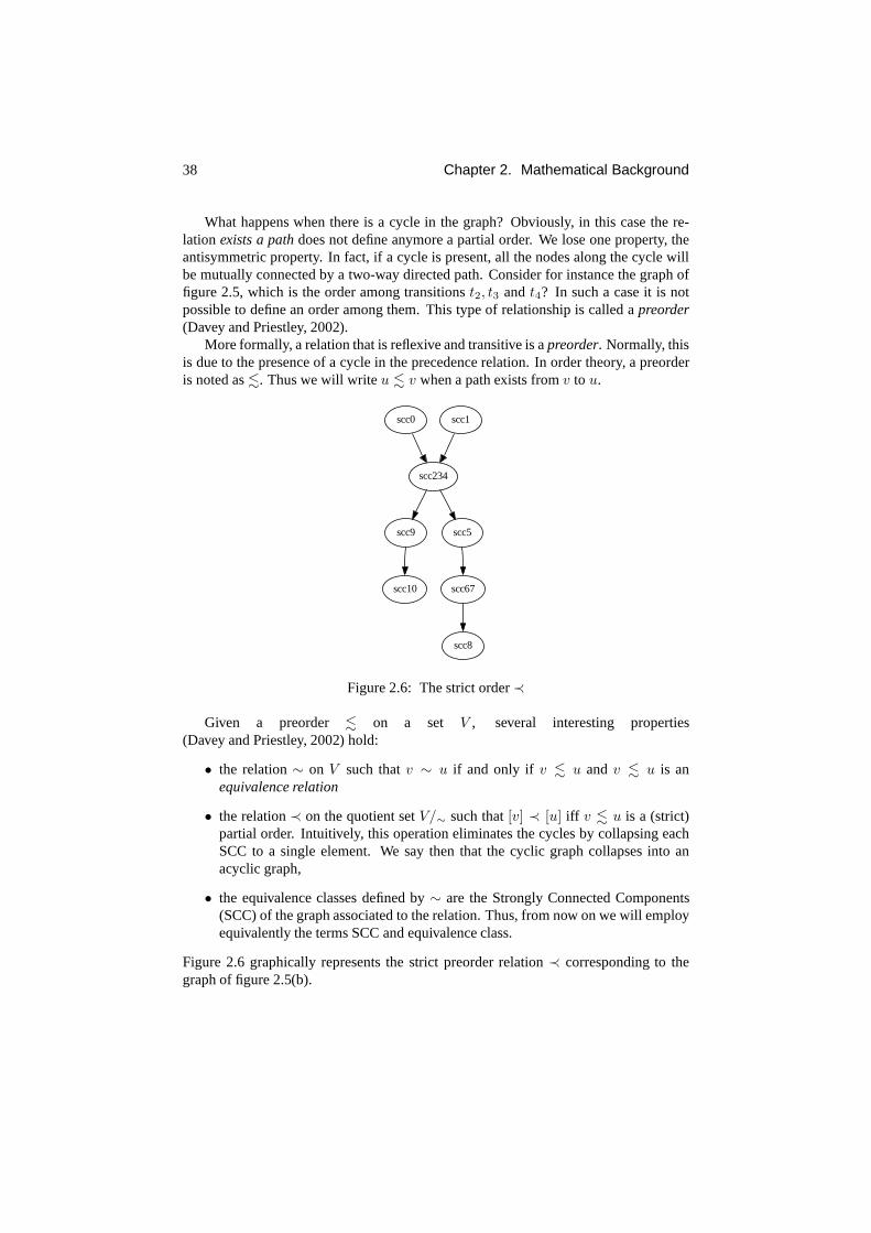
38 Chapter 2. Mathematical Background
What happens when there is a cycle in the graph? Obviously, inthis case the re-lation exists a pathdoes not define anymore a partial order. We lose one property,theantisymmetric property. In fact, if a cycle is present, all the nodes along the cycle willbe mutually connected by a two-way directed path. Consider for instance the graph offigure 2.5, which is the order among transitionst2, t3 andt4? In such a case it is notpossible to define an order among them. This type of relationship is called apreorder(Davey and Priestley, 2002).
More formally, a relation that is reflexive and transitive isapreorder. Normally, thisis due to the presence of a cycle in the precedence relation. In order theory, a preorderis noted as.. Thus we will writeu . v when a path exists fromv to u.
scc0
scc234
scc9 scc5
scc1
scc10 scc67
scc8
Figure 2.6: The strict order≺
Given a preorder . on a set V , several interesting properties(Davey and Priestley, 2002) hold:
• the relation∼ on V such thatv ∼ u if and only if v . u andv . u is anequivalence relation
• the relation≺ on the quotient setV/∼ such that[v] ≺ [u] iff v . u is a (strict)partial order. Intuitively, this operation eliminates thecycles by collapsing eachSCC to a single element. We say then that the cyclic graph collapses into anacyclic graph,
• the equivalence classes defined by∼ are the Strongly Connected Components(SCC) of the graph associated to the relation. Thus, from nowon we will employequivalently the terms SCC and equivalence class.
Figure 2.6 graphically represents the strict preorder relation ≺ corresponding to thegraph of figure 2.5(b).
Chapter 3
Related Work
In this chapter, we recall some related work. The problem dealt within this dissertationis indeed original, and, to the best of our knowledge, has been only marginally treatedby different disciplines like operations research, artificial intelligence, manufacturingengineering, and economics. Although a massive amount of work has been devotedto cope with different aspects of themake-or-buyor make-or-buy-or-collaborateprob-lems, to the best of our knowledge nobody has entirely treated them. In this chapter wewill summarise the literature close to our problem.
The chapter is organised as follows. In section 3.1, we will recall some basic con-cepts about auctions. Next, in section 3.2, we will thoroughly explain combinatorialauctions, a particular type of auctions. Then, in sections 3.3, we will introduce theproblems of supply chain scheduling and supply chain formation respectively. Next, insection 3.4, we will put in relation the work presented in this dissertation with respectto the state of the art.
3.1 Auctions
The most employed definition of auction is due to McAfee et. al(McAfee and McMillan, 1987): ”An auction is a market institution with an ex-plicit set of rules determining resource allocation and prices on the basis of bids fromthe market participants”.
Auctions play an important role in economics. In their most basic form, they areone of the ways in which various commodities, financial assets and concession rightsare allocated to individuals and firms, particularly in a market-oriented setting. Somevery famous examples of auction houses are Sotheby’s (Sotheby’s, 2007), Christie’s(Christie’s, 2007), and Ebay (Ebay, 2007).
The introduction and use of auctions is motivated by the factthat the value of anitem (or of a set of items) is often not known a-priori. Then, an auction is a way to“let the market decide” the value associated to the item. It is a very flexible mechanismthat is employed with several different variations. Furthermore, it is dynamic, since itallows a meaningful interaction between buyers and sellers. From our point of view,
39
40 Chapter 3. Related Work
the distinguishing feature of auctions is that they supportfull automation. In fact, theyare a mechanism with predetermined rules. Hence, they are ideal for computer imple-mentation. Finally, they are in most cases economically efficient (Milgrom, 2004).
3.1.1 Taxonomy of Auctions
Klemperer (Klemperer, 2004) classifies auctions in four basic groups based both on themodality the auction is run with and on the associated payment rule:
(1) theascending-bidauction, also known as English or Open-outcry;
(2) thedescending-bidauction, also known as Dutch;
(3) thefirst-price sealed-bidauction; and
(4) thesecond-price sealed-bidauction, also known as Vickrey auction.
In the ascending-bid auction, the price is raised successively until only one bidder re-mains. Such bidder wins the object and pays the final price.There are two variants ofthis auction. One (called Japanese) considers that the price is raised by the auctioneer,and the bidders that are not willing to pay the correspondingprice at a given round quitthe auction. The other one, known as English, let the bidderscall out the prices.
The descending auction works in exactly the opposite way, the price starts at a veryhigh price and it is successively decremented until some bidder expresses his willing-ness to accept that price.
In the first-price sealed-bid auction, all the bidders submit their offer without seeingthe other bidders’ offers. The bidder offering the highest bid wins paying his bid (thatis the highest price, whereby the namefirst-price).
In the second-price sealed-bid, the process is similar, with the exception that thebidder pays the price offered in the second highest bid, whereby the namesecond price.
Another classification can be done based on the number of buyers and sellers,namely:
• direct auction when there is one seller and multiple buyers;
• reverseauction when there is one buyer and multiple sellers. In thiscase the itemat auction is bought and not sold; and
• doubleauction when there are multiple buyers and multiple sellers.
Finally, a classification can be done based on the quantity ofitems sold/bought andon the features of the items (i.e. price is not the only discriminant of the value associatedto an item). In this case we shall refer tomultidimensional auctions. There are differenttypes of multidimensional auctions:
• multi-unit auctions when multiple identical items are bought/sold;
• multi-attributeauctions when the value associated to an object is determined bya set of features (shipping time, quality, and so on); and

3.2. Combinatorial Auctions 41
• multi-item or combinatorialauctions when multiple distinguishable items arebought/sold.
There exists a lot of hybrid auctions joining the features ofdifferent auction classes.In particular, very relevant to our work are (Cramton et al.,2006):
• combinatorial reverse auctions;
• multi-unit combinatorial reverse auctions.; and
• multi-unit combinatorial auctions.
Since combinatorial auctions (CAs) are of central importance in our work, in whatfollows we provide a detailed account on the state-of-the-art in CAs.
3.2 Combinatorial Auctions
A combinatorial (reverse) auction. (Cramton et al., 2006) is an auction where bidderscan sell (buy) entire bundles of goods in a single transaction. Although computation-ally very complex (Sandholm et al., 2002), the fact that bidders can express their prefer-ences over bundles of goods may help an auctioneer obtain better deals. In fact, buyingitems in bundles has the great advantage of eliminating the risk for a bidder of not be-ing able to sell/buy complementary items at a reasonable price in a follow-up auction(think of a combinatorial auction to acquire a pair of shoes,as opposed to two con-secutive single-item auctions for each of the individual shoes). Indeed, combinatorialauctions may lead to more efficient allocations whenever complementarities among thegoods at auction hold. For a detailed survey on CAs refer to (Cramton et al., 2006;de Vries and Vohra, 2003; Kalagnanam and Parkes, 2003).
CAs have a high potential to be employed as an allocation mechanism in a widevariety of real-world domains. They have been proposed to beemployed for allo-cating loads to trucks in the transportation market (Caplice and Sheffi, 2006), routesto buses (Cantillon and Pesendorfer, 2006), goods/services to buyers/providers in in-dustrial procurement scenarios (Bichler et al., 2006), airport arrival and departure slots(Ball et al., 2006), and radio-frequency spectrum for wireless communications services(Pekec and Rothkopf, 2003). Walsh in (Walsh et al., 2000) employed them for supplychain formation.
The study of the mathematical, game-theoretical and algorithmic properties of com-binatorial auctions has recently become a popular researchtopic in AI. This is not onlydue to their relevance to important application areas such as electronic commerce orsupply chain management, but also to the range of deep research questions raised bythis auction model.
In the last decades, different topics related to CAs have been considered, namelythe design of auction mechanisms, bidding languages, and algorithms for the WinnerDetermination Problem. In the following sections, we summarise the most relevantcontributions on those topics.

42 Chapter 3. Related Work
3.2.1 Mechanism Design
Auction theory studies the formal properties of auctions asshown in the sur-veys of (Krishna, 2002) and (Milgrom, 2004). Nonetheless CAs have recentlyattracted the attention of economists and game theorists. Associated to auc-tion theory is also the design of auctionmechanisms, devoted to studyhow torun an auction in order to guarantee some economic properties such as, for in-stance, efficiency, incentive compatibility, individual rationality, etc. For instance,(Ausubel and Milgrom, 2006b), (Parkes, 2006), (Ausubel andMilgrom, 2006a),(Cramton, 2006), (Ausubel et al., 2006), and (Land et al., 2006) describe somemechanisms for CAs.
3.2.2 Bidding Languages
Bidding is the process of transmitting one’s valuation function over the set of goods onoffer to the auctioneer (or rathersomevaluation function — the bidders are of coursenot required to reveal their true valuation —). In principle, it does not matter how thevaluation function is being encoded, as long as sender (bidder) and receiver (auctioneer)agree on the semantics of what is being transmitted,i.e. as long as the auctioneer canunderstand the message(s) sent by the bidder. Indeed, it is possible to fully specifyan auction mechanism (allocation and pricing rules) without reference to a concretebidding language. In practice, however, the choice of a bidding language is of centralimportance.
Early work on combinatorial auctions has typically ignoredthe issue of bidding lan-guages. The standard assumption used to be that if a particular bidder submits severalatomic bids (a bundle together with a proposed price), then the auctioneer may acceptany set of bids from that bidder for which the bundles do not overlap, and charge thesum of the specified prices. This is now sometimes called theOR language. But otherinterpretations of a set of atomic bids are possible. For instance, we may take it to meanthat the auctioneer may accept at most one bid per bidder; this is now known as theXOR language.
The first systematic study of bidding languages is due to Nisan (Nisan, 2006) (anearly version (Nisan, 2000) appeared in 2000). Nisan’s papers provide an excellentintroduction to the topic and clarify a number of issues thathad previously remainedsomewhat fuzzy. Nisan classifies several types of bidding languages, providing expres-siveness results for each of them. At the basis of his exposition lies the concept ofatomic bid. Formally, an atomic bid is a pair(S, p), whereS is a subset of the items atauction, andp is the price a bidder is willing to pay to obtain the goods inS. By com-bining in different ways atomic bids we obtain several bidding languages. The mostwidely employed are:
• OR. Each bidder submits an arbitrary number of atomic bids. Theauctioneer isallowed to accept any disjoint subset of them.
• XOR. Each bidder submits an arbitrary number of atomic bids. Theauctioneer isallowed to accept at most one among them.

3.2. Combinatorial Auctions 43
• OR-of-XOR. Each bidder can submit any number of XOR bids. The auctioneer isallowed to accept any subset of these bids.
• XOR-of-OR. Each bidder can submit an arbitrary number of OR bids. The auc-tioneer is allowed to accept at most one of these bids.
Consider the following example explaining the semantics ofOR andXOR bids.
Example 3.1. Say that the set of goods at auctions is{A, B, C}. Then, we have:
• OR: ({A}, 3) OR ({B, C}, 3) means that if the bidder is allocated{A, B, C},then he will pay 6.
• XOR: ({A}, 3) XOR ({B}, 3) XOR ({A, B}, 5) means that if he is allocated{A, B} he will pay 5 (not 6).
Another interesting paper about bidding languages is (Boutilier and Hoos, 2001),where Boutilier et al. present a logical bidding language that allows the expressionof complex utility functions in a natural and concise way. Inthis language bids aregiven by propositional formulae whose sub-formulae can be annotated with prices, thusallowing for a natural and concise formulation of bidders’ utility functions.
To the best of our knowledge, no bidding language has considered so far services ormanufacturing operations as entities that can be traded. Asexplained in chapter 1, in or-der to apply combinatorial auctions to themake-or-buyof make-or-buy-or-collaboratedecisions, it is required to predicate about manufacturingoperations and services acrossthe supply chain.
3.2.3 Winner Determination Problem
Connected with the introduction of combinatorial auctionsis the winner determina-tion problem (WDP). Winner determination is the problem, faced by the auction-eer, of choosing which goods to award to which bidder so as to maximise its rev-enue. The winner determination for combinatorial auctionsis a complex computa-tional problem. Indeed, one of the fundamental issues limiting the applicability of CAsto real-world scenarios is the computational complexity associated to the winner de-termination problem. In particular, it has been proved thatthe WDP is NP-complete(Rothkopf et al., 1998). General IP solvers (Andersson et al., 2000) and special pur-pose algorithms (Sandholm, 2002; Fujishima et al., 1999; Leyton-Brown et al., 2000)have been employed to solve the WDP, but it is well known that ageneral solver thatperforms well in all situations does not exist. For an extended review on the winnerdetermination problem and related issues refer to (Lehmannet al., 2006; Muller, 2006;Sandholm, 2006b).
Here we aim at presenting the traditional ILP (see section 2.1.2) formulation em-ployed to model the combinatorial auction winner determination problem, given that itscomprehension is required to understand the remaining of the dissertation.

44 Chapter 3. Related Work
ILP formulation for the Combinatorial Auction WDP
Say that an auctioneer wants to selln goods. Each good is denoted asgi, where1 ≤ i ≤n. In a combinatorial auction bidders can sendall-or-nothingoffers over a set of goods.Say that each of them bidders participating in the auction only submits one bid1 bj ,1 ≤ j ≤ m. Each bid is represented by a pairbj = (Sj , pj) such thatpj is the price thatthe bidder is willing to pay for obtaining the set of goodsSj . How can the auctioneerselect the bids that maximise his revenue? This problem can be easily modelled bymeans of Integer Programming (refer to section 2.1.2 for a detailed explanation). Weassociate to each bidbj a binary decision variablexj ∈ {0, 1} that takes on value1if bid bj is selected, and0 otherwise. Then, the function that the auctioneer wants tomaximise is his revenue, namely:
m∑
j=1
xjpj (3.1)
that is theobjective functionof the integer program.Additionally, we have to make sure that each good is sold to atmost one bidder
since the auctioneer only owns one copy of each good. Thus, weemploy coefficientscij to model that either goodgi is required in bidbj (cij = 1), or not (cij = 0). Then,the following constraints must hold:
m∑
j=1
cijxj ≤ 1 1 ≤ i ≤ n (3.2)
In what follows we list some attempts carried out in the past to deal with the gener-ation of benchmarks for testing combinatorial auctions WDPalgorithms.
3.2.4 Test Suites
No real-world benchmark of CAs has been reported in the literature. Many effortshave been done so far to generate plausible data sets to be employed to test WDP al-gorithms. Some experiments have been run with human bidders(Banks et al., 1989).Nonetheless, as pointed out in (Leyton-Brown and Shoham, 2006), such data sets arenot useful for assessing the WDP computational complexity.In the absence of testsuites, it is common practice to artificially generate data sets. Some examples are(Fujishima et al., 1999; Boutilier et al., 1999; de Vries andVohra, 2003) for single-unitCAs, and (Leyton-Brown et al., 2000) for multi-unit CAs. Multi-unit CAs have alsobeen tested employing multidimensional knapsack problem benchmarks, borrowedfrom the operations research community. A more realistic approach to generate bidsis presented in (Leyton-Brown and Shoham, 2006), where complementarity relation-ships among goods are made explicit at bid generation time. Another realistic approachis taken in (An et al., 2005), where the authors design bidding strategies that efficiently
1We do this simplified hypothesis for the sake of comprehension. The extension to the OR or XOR biddinglanguage is easy (Lehmann et al., 2006).

3.3. Supply Chain Scheduling and Supply Chain Formation 45
identify desirable bundles in the framework of the transportation industry domain (fo-cusing therefore on single-round, first-price, sealed-bidforward CAs).
Finally, a master student has elaborated on subjects related to this thesis. Vinyals(Vinyals, 2007b; Vinyals et al., 2007a; Vinyals et al., 2007b) has implemented a verypowerful simulator of the behaviour of agents bidding in an MMUCA, and has testedthe performances of some of the algorithms presented in thisdissertation.
In what follows we change of subject and introduce the work inthe state-of-the-artrelated to supply chain scheduling and supply chain formation.
3.3 Supply Chain Scheduling and Supply Chain For-mation
In this section, we will talk about supply chain scheduling and planning, and supplychain formation. On the one hand, the problem of supply chainformation concerns theselection of the participants to the supply chain and the terms of the exchange, withthe purpose of maximising the efficiency of the supply chain.Informally, supply chainformation is the problem of decidingwho will supply what, who will do what, andwho will buy what. On the other hand, the problem of supply chain scheduling andplanning is more focused on the coordination among the different operations acrossthe supply chain with the purpose of minimising the cost of performing operations andtransportation, and the time required to perform all the operations. Informally, supplychain scheduling and planning is the problem of decidingwheneach agent within thesupply chain has to perform a given operation or job in order to finish all the operationsbefore a given deadline.
There is a fundamental difference between the problem of supply chain formationand the problem of supply chain scheduling and planning. Theformer deals with findinga set of supply chain partners, whereas the latter deals withthe problem of coordinatingthem. Nevertheless, the two problems are tightly connected. In fact, in order to ef-fectively select the participants to the supply chain, agents should make sure that thereexists a feasible scheduling of their operations. This is needed since each stakeholderalong the supply chain:
• provides resources subsequently employed by other stakeholders; or
• employs or consumes resources previously produced by otherstakeholders; or
• produces resources subsequently employed by other stakeholder, requiring as in-puts resources previously supplied by other stakeholders.
Then, the selection of partners can be greatly improved if the feasibility of the schedul-ing is taken into account.
In the literature there have been many attempts to solve the problem of supply chainplanning and scheduling and some attempts dealing with the supply chain formationproblem. However, to the best of our knowledge, no attempt tosolve the problem ofsupply chain formation taking into account the feasibilityof the scheduling has beendone so far.
46 Chapter 3. Related Work
3.3.1 Supply Chain Scheduling and Planning
There exist two approaches to supply chain planning and scheduling (Lau et al., 2006):centralisedanddistributed.
The Centralised Approach
The centralised approach to supply chain scheduling has been investigated for manyyears. In this approach a central authority collects all theinformation from the peersand then computes the optimal planning (Cohen and Lee, 1988;Ertogral et al., 1998;Sabri and Beamon, 2000; Jayaraman and Pirkul, 2001; Lee et al., 2002). A good sur-vey on centralised planning can be found in (Erenguc et al., 1999).
The information required to optimise the scheduling may either be centralised ordistributed, according to the nature of the problem. For instance, inside an enterprisethere may be a central repository of information, whereas ina consortium of enterpriseseach firm holds its private information. The information that must be provided in or-der to compute the planning concerns the production features of the participants (therequired time to perform an operation, the associated cost,the precedence relationshipsamong operations, and so on). One of the firm acts as a coordinator, and, after receivingthe production data, computes an optimal plan, that is subsequently communicated tothe other supply chain stakeholders. In this approach, there must be information sharingamong the supply chain stakeholders in order to obtain an efficient plan.
Many methods have been proposed to solve the underlying plan-ning problem, for instance metaheuristics (Kallrath, 2002), stochasticalgorithms (Alonso-Ayuso et al., 2003), or mixed-integer programming(Gaonkar and Viswanadham, 2001).
The centralised approach suffers from some drawbacks. Firstly, some firms may bereluctant to share very sensitive internal information. Secondly, the computational timerequired to solve even small instances is huge. Finally, thecentralised approach makesit difficult to react to fails and breakdowns across the supply chain. In case some ofthese events occur, the scheduled plan must be recomputed from scratch.
The Distributed Approach
In the distributed approach, the decisions about the scheduling are taken locally. Thatis, a supply chain stakeholder builds its schedule relying on the communications with itsneighbours along the supply chain. The decision is based on the local information andobjectives of each supply chain stakeholder. The interactions among the supply chainparticipants continue until a global scheduling is found orsome termination conditionis met.
The major advantages of the distributed approach versus thecentralised one are:
• the information is shared only at a local level;
• the computational complexity of the problem is reduced, since the problem solvedlocally by each supply chain stakeholder is by far less difficult than the globaloptimisation problem; and

3.3. Supply Chain Scheduling and Supply Chain Formation 47
• since enterprises act locally, the capacity of reacting to breakdowns or shortcom-ings is increased with respect to the centralised approach.
Many methods have been proposed to solve the scheduling problem with a decen-tralised approach. For a good review, refer to (Lau et al., 2006). The most celebrateddistributed approach for centralised supply chain scheduling and planning has beenthe Contract Net Protocol (CNP), along with all its variants. In his original formula-tion, the CNP specifies a bidding approach that enables task allocation among mul-tiple agents (Smith, 1980). The multi agent system (Wooldridge and Jennings, 1995)based approach has been widely employed in the past as well (Collins, 2002;Zhang, 2002; Reis et al., 2001; Lee et al., 2003; Wagner et al., 2003; Lau et al., 2006;He et al., 2003; Norman et al., 2004).
The distributed approach suffers as well from some drawbacks. The main short-comings regard the feasibility and optimality of solutions. It has been shown(Jennings and Wooldridge, 1998) that, since agents act and reason locally, they disre-gard the other agents’ constraints and the global performance of the supply chain.
To conclude, choosing between a centralised or a distributed approach strongly de-pends on the problem to be solved and on the availability of computational resources.
3.3.2 Supply Chain Formation
Very little work has been devoted to the problem of automating supply chain forma-tion. In this chapter, we will not consider the literature onnon-automated supply chainformation because its contributions stem from the areas of economics and negotiationrather than from optimisation. Thus, it is out of the scope ofthe dissertation.
Supply chain formation studies the problem of automating the process of determin-ing the supply chain partners, under the assumption that theinformation required by thedecision making process is decentralised.
In the area of supply chain formation two approaches have been considered as well,namely the centralised and the distributed approach.
The Centralised Approach
As far as we are concerned, little effort has been devoted to the centralised approach tothe supply chain formation problem.
A significant attempt to provide a mechanism to select the right business partners ina supply chain has been undertaken by (Gaonkar and Viswanadham, 2005). This workis probably at the edge between supply chain planning and supply chain formation.This very interesting paper focuses on the problem from a real-world point of view:what happens when there is a roll-over of products in a market? Should a firm maintainthe same business partners? Should it change them? The authors provide a mixedinteger programming formulation of the underlying decision problem. This approachsuffers from some limitations:
(1) it is not completely automated, because the interactionbetween the supply chainstakeholders is performed through an Internet-enabled platform;

48 Chapter 3. Related Work
(2) there is no communication language among the supply chain stakeholders (like,for instance, a bidding language); and
(3) it has a high computational cost and subsequent poor scalability.
However, it substantially differs from our approach, sinceit is not based on a marketmechanism. It is more a static decision support system to help strategic decision makingunder particular market conditions.
In (Walsh, 2001; Walsh et al., 2000), Walsh et. al introduce combinatorial auctionsfor supply chain formation. These represent an extension ofcombinatorial auctions inwhich a whole supply chain is negotiated via an auction. In such a context, askers,sellers and manufacturers participate and submit bids within the same auction. In orderto cope with this new auction Walsh et. al introduce the Task Dependency Network(TDN), a network representing all the producer/consumer relationships among the bid-ders. We consider that this work has dealt with a problem verysimilar to ours. In factboth our and their work:
• are built upon a market-based mechanism, namely combinatorial auctions;
• explicitly represent producer-consumer relationships holding across the supplychain; and
• model resource contention (i.e. the fact that in the system there are less resourcesavailable than the overall required ones).
However, as explained in section 1.4.2, Task Dependency Networks and combinatorialauctions for Supply Chain Formation are limited along several dimensions: they do notpossess the expressiveness, computational, and formal analysis tools required to dealwith themake-or-buy-or-collaboratedecision problem.
Collins et. al in (Collins, 2002; Babanov et al., 2003) deal with a problem similarto the supply chain formation introducing time and precedence constraints. Howeverthey do not explicitly model the multiple levels within a supply chain and the resourcecontention across it. They also provide a bidding language including information aboutthe time required to perform operations.
Finally, Norman et. al (Norman et al., 2004) describe a combinatorial auction toform virtual organisations. They also provide an advanced bidding language for ex-pressing offers in which the time dimension is considered aswell. Although very in-novative, we find that its applicability to the problem of supply chain formation is lim-ited since neither resource contention nor the producer-consumer relationships presentacross a supply chain can be modelled.
The Distributed Approach
Distributed approaches to supply chain formation are not soclosely related to our work.However, we will point out the two most relevant works in the field that employ a marketbased mechanism.
Rosenschein and Zlotkin in (Rosenschein and Zlotkin, 1994;Zlotkin and Rosenschein, 1996) introduce Task Oriented Domains (TODs). A

3.4. Conclusions 49
TOD is a set of tasks that must be completed, and a cost function over bundles of tasks.They fix a set of negotiation rules and provide some theoretical results on the propertiesof the negotiation outcome.
Walsh and Wellman in (Walsh and Wellman, 2003) provide a decentralised versionof the auction mechanism provided in (Walsh et al., 2000), which is based on a variationof the Contract Net Protocol.
We stress that both approaches suffer from limitations. On the one hand, TODsdo not incorporate nor implicitly neither explicitly the dependencies among operationsacross a supply chain, whereas the model in (Walsh and Wellman, 2003) suffers fromthe same expressiveness, computation and formal analysis shortcomings as combinato-rial auctions for supply chain formation do.
3.4 Conclusions
Little work has been done so far to solvemake-or-buyor make-or-buy-or-collaboratedecisions with a centralised market-based approach. Many papers have focused on sim-ilar problems though none of them captures all the requirements expressed in sections1.4.1 and 1.4.2.
Our work is placed somewhere in betweencentralised supply chain planningandcentralised supply chain formation. Our work is not entirely included in the field of sup-ply chain formation because we do not only assess the participants to a supply chain,but we also provide a feasible sequence of supply chain operations to perform. Anal-ogously, our work is not completely included in the field of supply chain schedulingsince the participants to the supply chain are not fixed a-priori, but determined on thefly based on a market mechanism. Furthermore, we do not need toinclude the timedimension into the problem to provide a feasible schedule. In fact, the precedence rela-tionships among operations are implicitly represented in the formalism that we employto model resource contention at each level of the supply chain.
Summarising, in the state of the art we find solutions to both supply chain schedul-ing and planning and to supply chain formation problems. However, none of the solu-tions we are aware of possesses all the features required to solve bothmake-or-buyandmake-or-buy-or-collaboratedecision via a market-based approach.
(1) As thoroughly explained in sections 1.4.1 and 1.4.2,combinatorial auctionslackof the possibility to express manufacturing operations, orequivalently productionrelationships among the goods at auction. However, they provide a good modelto build upon because they allow to express complementarities among the goodsat auction (Cramton et al., 2006); they can count on theoretically well-foundedbidding languages (Nisan, 2006), and there have been significant contributions tothe study of their winner determination problem (Lehmann etal., 2006).
(2) As detailed in section 1.4.2, combinatorial auctions for supply chain formationand the associated Task Dependency Networks help negotiating manufacturingoperations. However, they suffer fromformal, computational, andexpressivenesslimitations.

50 Chapter 3. Related Work
(3) We deem that distributed approaches are not suitable to our problem. In fact,to the best of our knowledge, they do not guarantee nor optimality nor feasi-bility. The literature in combinatorial auctions has thoroughly demonstrated theefforts in finding optimal solutions to the winner determination problem. In to-day’s business world, to provide methodologies that sacrifice optimality when bigquantities of money are in play is a risky business.
Chapter 4
MUCRAtR
In this chapter we deal with themake-or-buydecision problem when complementaritiesamong goods hold at the bidders’ side. With this aim, we introduce a new type of com-binatorial auction, theMulti-unit Combinatorial Reverse Auction with transformabilityRelationships among goods (MUCRAtR), extending traditional combinatorial auctions.We also provide a mapping of the MUCRAtR winner determination problem to an opti-misation problem on Place/Transition Nets (PTN). Such a mapping allows to efficientlysolve the WDP for some problem classes, and provides a set of powerful formal toolsfor describing the underlying optimisation problem.
This chapter is organised as follows. In section, 4.1 we introduce the problem weaim at solving and informally outline the proposed solution. In section 4.2, by meansof some examples and intuitions, we introduce the limitations associated to CAs withrespect to themake-or-buydecision problem in a combinatorial scenario. In section4.3, we introduce a formalism, based on PTN, that overcomes part of such problems.In section 4.4 we extend PTN in order to amend the expressiveness shortcomings of thePTN model. In particular, we introduce a new type of PTN called Weighted Place Tran-sition Net(WPTN). Moreover, we define a new reachability problem over WPTN, theConstrained Maximum Weight Occurrence Sequence Problem(CMWOSP). In section4.5, relying on WPTNs, we succeed in formally representing an auctioneer’s internalproduction and cost structure along with the set of receivedoffers from bidders under aunified formalism. Building upon such framework, we formally define the WDP for thenew auction as a particular CMWOSP. In section 4.7, we prove that the CMWOSP, andthus the WDP formalised in section 4.6, can be solved by meansof IP under suitableconditions. Finally, section 4.8 draws some comments and concluding remarks.
4.1 Beyond Combinatorial Auctions
In the introductory chapter we mentioned that we are dealingwith two main issuesin this dissertation. The first one is the automation ofmake-or-buydecisions across thesupply chain, and the second is the automation ofmake-or-buy-or-collaboratedecisionsacross the supply chain. In this chapter we focus on themake-or-buydecision problem,
51

52 Chapter 4. MUCRAtR
namely the problem of selecting what to produce in-house andwhat to outsource inorder to obtain some required goods. We argued in section 1.4.1 that this concern isreasonable because the cost of the raw materials plus the cost of the manufacturingoperations could eventually be higher than the cost of already-made goods. As an ad-ditional constraint, we require that the complementarities among goods on the bidders’side are taken into account: bidders should be allowed to composeall-or-nothingoffersover bundles of goods.
In section 1.4.1, through the example of theGrandma & cofirm, we showed thatthemake-or-buydecision problem represents a challenging problem in a scenario withcomplementarities among the goods. We highlighted thatGrandma & corequires acomplex decision support system along with a combinatorialnegotiation mechanismthat helps it in detecting the cost-minimising buying configuration and the internal op-erations to perform in order to obtain the finally required goods.
For this reason, we decided to build upon combinatorial auctions to cope with themake-or-buydecision problem. We recall that the distinguishing feature of combinato-rial auctions is that bidders can submitall-or-nothingoffers over bundle of goods. Thisallows to mitigate the risks connected with markets with strong complementarities, likefor instance depressed bidding1.
Unfortunately, as we thoroughly showed in section 1.4.1, some limitations preventthe application of combinatorial auctions to themake-or-buydecision problem. Thatis mainly due to two types of limitations:expressivenessand winner determinationproblem. We recall in table 4.1 the limitations of combinatorial auctions thoroughlyexplained in section 1.4.1.
Hence, in this chapter we extendMultiunit Combinatorial Reverse Auctions(MU-CRA)2 in order to overcome the intrinsic limitations of CAs for dealing with themake-or-buy decision problem. The resulting auction model is calledMulti-unit Combina-torial Reverse Auction with transformability Relationships among goods (MUCRAtR).This new auction type allows a buyer/auctioneer to express and communicate to biddersits internal production structure and its final requirements. Bidders can then formulateappropriate offers and send them back to the auctioneer. Upon receiving the offers,an auctioneer can determine, by means of a public selection rule, the cost minimisingcombination of bids along with the internal operations leading to its final requirements.
Then, firstly we try to model an auctioneer’s internal manufacturing operations bymeans of Place Transition Nets (PTNs, thoroughly describedin section 2.3). They per-fectly represent the manufacturing operations by specifying the quantity of resourcesboth required an produced by each manufacturing operation.Furthermore, they natu-rally model the producer/consumer relationships holding among them. Then, the PTNrepresenting the internal manufacturing operations fulfills requirement (1) in table 4.1.
Next, we incorporate the offers received by the auctioneer into the PTN encodingthe auctioneer’s production structure. This idea is based on the intuition that the selectedoffers inject goods into the auctioneer production process: without ingredients it is notpossible to produce pies. This solves issue (3) in table 4.1.
1Depressed bidding is a phenomenon associated to the fact that bidders may risk to obtain only a part ofa set of complementary goods, and therefore bid less aggressively.
2We recall that a MUCRA is simply a combinatorial reverse auction in which multiple copies of each itemare auctioned3 (Sandholm, 2002).

4.1. Beyond Combinatorial Auctions 53
TYPE REQUIREMENTS
Expressiveness
(1) specification of the internal manufactur-ing operations and the producer/consumerrelationships among them
(2) specification of an auctioneer’s final re-quirements
(3) relationships among the manufacturingoperations, the auctioned goods, and thereceived bids
(4) specification of an auctioneer’s internalcost structure
WDP(5) information about which in-house opera-
tions to perform and in which order
Table 4.1: Summary of requirements for themake-or-buydecision problem.
More in details, we build two PTNs: one representing the internal manufacturingoperations of an auctioneer, that we namePTNI (I from Internal), and another oneextendingPTNI to incorporate offers, calledPTNE (E from Extended).
The dynamic behaviour of PTNs serves to describe the set of possible outcomes ofa MUCRAtR. In particular, PTNs can naturally model:
(1) the preconditions of each manufacturing operation (therequired inputs must bepresent);
(2) the resources consumed and produced by each manufacturing operation;
(3) the quantity of resources injected into the system when an offer is selected; and
(4) the quantity of resources available to an auctioneer after performing a given man-ufacturing operation.
According to item (4) in the list above, an auctioneer can model its resource availabilityat any step of its manufacturing process. Consequently,PTNE can compactly encodethe outcomes (in terms of finally available resources) of allthe possible decisions anauctioneer may take4. The encoded information concerns the level of resources avail-able at the end of a production process fed by a set of offers and composed of a sequenceof internal operations. Furthermore, the rules governing the dynamics of PTNs enforcethat each of the possible decisions is implementable, i.e. all the manufacturing opera-tions are run in the correct order and only if the required input resources are provided.
4Notice that by decision we mean the selection of a set of offers and of a set of internal manufacturingoperations.

54 Chapter 4. MUCRAtR
However, an auctioneer is not simply interested in choosingthe bids and the internaloperations leading to a satisfactory level of available resources. Above all he is inter-ested in minimising its costs while doing this. Unfortunately, PTNs allow to expressneither the cost associated to performing manufacturing operations nor the cost asso-ciated to selecting a set of bids. Due to this expressivenesslimitation, we decided toextend the notion of PTN to incorporate the cost associated to a manufacturing opera-tion and the cost associated to a bid. Such extension, calledWeighted Place TransitionNets (WPTN), allows associating a cost to each transition of a PTN.
With this tool at hand, we firstly associate a cost to each transition ofPTNI . Thiscreates a WPTN allowing to reason about the manufacturing operations internal to anauctioneer. I name such WPTNTransformability Network Structure(TNS). It incor-porates the following information about an auctioneer’s internal manufacturing opera-tions:
(1) the required input goods;
(2) the produced output goods;
(3) the cost associated to each operation; and
(4) the eventual producer/consumer relationships with other operations.
By means of a TNS, an auctioneer can also compactly communicate to bidders all thepossible RFQ configurations leading to its final requirements. Summarising, the infor-mation contained in a TNS along with the auctioneer’s finallyrequired goods provideto bidders sufficient information to compose meaningful offers. This overcome require-ment (2) of table 4.1.
As mentioned above, our strategy shall be to map the internalmanufacturing op-erations and the received offers into a PTN (PTNE). If we associate a cost to eachof its transitions, we obtain a WPTN that provides a unified description framework forthemake-or-buydecision problem. I call such extensionAuction Netbecause it permitsto encode the information about an auctioneer’s internal production and cost structuresand about the offers it receives. The formal language offered by anAuction Nethelpsfulfill expressiveness requirements (1), (3) and (4) of table 4.1.
By means of anAuction Netan auctioneer can compactly express the outcome ofany of its possible decisions (acceptance of some bids and execution of some internaloperations), and also quantify the cost associated to each of such outcomes. Further-more, theAuction Netallows to incorporate the information about an auctioneer’s initialstock.
We recall that the goal of the auctioneer is selecting a cost minimising outcomefulfilling its final requirements. This can be achieved only if he can express constraintsover possible outcomes. Then, the last requirement for expressing the decision problemis allowing an auctioneer to express constraints over the set of possible outcomes.
Against this background, the MUCRAtR winner determinationproblem can bestated as a problem over anAuction Net(a WPTN), where the goal is minimising thecost associated to a sequence of steps that brings to a final state fulfilling some con-straints. Then, we define a new optimisation problem on WPTNs: the Constrained

4.2. The problem 55
Maximum Weighted Occurrence Sequence Problem(CMWOSP). The objective of aCMWOSP is finding a cost minimising sequence of steps leadingto a final state fulfill-ing a set of constraints. This provides a solution to requirement (5) in table 4.1.
Notice that the result of a CMWOSP is afiring sequence, i.e. an ordered sequence oftransitions. This reflects a critical feature of themake-or-buydecision problem. An auc-tioneer cannot run its internal manufacturing operations in a random order. Because ofproducer/consumer relationships among manufacturing operations, an auctioneer mustbe aware of the implementation order. For instance, ifGrandma & codecides to onlybuy the basic ingredients and to perform all the manufacturing operations internally, itcannot perform theBakingoperation before theMake Doughor Make Filling opera-tions, since the latter ones provide the inputs to the formerone (cf. figure 1.1).
Then, the definition of the winner determination problem does not only assess theoptimal set of goods to buy, but also the optimal ordered sequence of in-house opera-tions to perform in order to obtain the goods finally requiredby the auctioneer.
Two direct benefits stem from the mapping of the MUCRAtR WDP toWPTNs.Firstly, it is possible to directly import all the PTNs analysis tools and theoretical re-sults and apply them to our problem. This provides the techniques for dealing withrequirement (5) in table 4.1. In fact, we manage to model, fora wide class of problems,the WDP via integer programming (see section 2.1.2), and efficiently solve it by meansof black-box solvers as ILOG CPLEX (ILOG, 2007) or GNU GLPK (Makhorin, 2001).
4.2 The problem
In what follows we further specify the extensions to CAs needed for dealing with themake-or-buydecision problem. With this aim we extend example 1.1 in chapter 1. Werecall that the example was aboutGrandma & co, a company devoted to produce andsell apple pies. According to the example, the marketing department atGrandma &co has forecast a sale of two hundreds apple pies within the nextmonth, and thereforeGrandma & costarts an automated sourcing process.Grandma & coopts for runninga combinatorial auction to source the required ingredients. However, as explained insection 1.4.1, besides inviting providers of basic ingredients (butter, sugar, flour, apples,margarine), Grandma & coinvites providers of intermediate goods (dough, filling),and even of final goods (apple pies). The production management department aims atevaluating the opportunity to outsource part of the production process.
Unfortunately,Grandma & cofaces a decision problem that cannot be solely treatedby means of combinatorial auctions because of the intrinsiclimitations listed in table4.1. In example 4.1 we provide an extended version of example1.1 that explicitlyillustrates such limitations.
Example 4.1. The data characterising theGrandma & co’s decision problem are:
(1) The cost of its internal manufacturing operations:
(a) A Make Doughoperation costse 5 each time it is carried out. It requiresone unit ofbutter, three units ofsugar, and two units offlour as inputs; andit produces two units ofdoughas output.

56 Chapter 4. MUCRAtR
(b) A Make Fillingoperation costse 6 each time it is carried out It requires oneunit of flour, eight units ofapple, and two units ofmargarineas inputs; andit produces two units offilling as output.
(c) A Bakingoperation costse 14 each time it is carried out. It requires fourunits ofdoughand four units offilling as inputs; and it produces four unitsof apple pieas output.
(2) A sale forecast of 200 apple pies. This represents the final requirements ofGrandma & co.
(3) A stock of one hundred units offloor and two hundreds units ofsugar.
Then, if Grandma & cointends to run a combinatorial auction and to invite all itsproviders, it must be able to
• send them a request for quotes (RFQ) containing the number ofrequired units foreach good; and
• once received all bids, it must be able to determine which bids to accept andwhich internal manufacturing operations to perform in order to obtain the 200apple pies.
Unfortunately, life is not that easy forGrandma & co. Firstly, it is not possible to apriori establish how many units of each good the auctioneer (Grandma & co) requires.In fact, this depends on the production plan, that can only bedecided upon receivingthe offers. Secondly, once received all bids,Grandma & coneeds a winning rule for theoptimal, efficient and automatic selection of the best set ofbids and in-house operations.In the two following sections we illustrate the first and second problem.
4.2.1 Communicating the RFQ
In a traditional Multi-Unit Combinatorial Reverse Auction(MUCRA) scenario, aRe-quest for Quotation(RFQ) (Reyes-Moro et al., 2003) expresses the number of requiredunits for each good. However, whenever an auctioneer (Grandma & co) facesmake-or-buydecision problems, it happens that the requirement sent to bidders (the RFQ) is notequivalent to the quantity of goods that the auctioneer actually requires (the 200 applepies). When internal manufacturing operations are taken into account, an auctioneerhas to distinguish between the objective quantity of goods at the end of its productionprocess and what to ask providers for. This occurs because anauctioneer (Grandma &co) can opt for several, possible buying options and several, possible levels of internalproduction. All these options differ in the number of required units and in the level ofinternal production. For instance,
• if Grandma & codecides to buy only already-made pies without producing any-thing, then it must ask providers offers for two hundred units of apple pies. Thisresults in the RFQ expressed in table 4.2(a) and in the internal operations quanti-fied in table 4.2(b).

4.2. The problem 57
Resource Required Unitsbutter 0sugar 0flour 0
apples 0margarine 0
dough 0filling 0
apple pies 200
Resource Required Unitsbutter 100sugar 500flour 300
apples 800margarine 200
dough 0filling 0
apple pies 0
(a) Request for quotes for apple pies only. (c) Request for quotes for basic ingredients only.
Operation QuantityMake Dough 0Make Filling 0
Baking 0
Operation QuantityMake Dough 100Make Filling 100
Baking 50
(b) Internal operations to perform. (d) Internal operations to perform.
Table 4.2: Request for quotes for different scenarios.
• if Grandma & codecides to produce everything in house, then it must requirefor each ingredient the quantity needed for producing 200 apple pies, and mustperform theMake Dough, Make Filling,andBakingoperations as many timesas required. This corresponds to the RFQ expressed in table 4.2(c) and in theinternal operations quantified in table 4.2(d).
It is easy to understand whyGrandma & cocannot completely specify its exact require-ments a-priori (limitation (2) in table 4.1). The number of acquired units will dependon the received offers.
In order to overcome such difficultyGrandma & coshould be able to communicateto bidders its internal production relationships along with the producer/consumer rela-tionships among them (limitation (1) in table 4.1). When bidders have this informationavailable,Grandma & cosimply has to communicate to bidders the quantity of eachgood it aims at obtaining at the end of the production process(in our case two hundredapple pies). The bidders can then infer the required quantity for each good (limitation(2) in table 4.1).
4.2.2 Selecting the optimal decision
Even under the hypothesis thatGrandma & cowas able to uniquely communicate itsrequirements to bidders, once received the bids it would notbe able to decide whichbids to accept and which internal operations to perform in order to minimise its costsand to obtain the 200 apple pies. More importantly, it would not have any public rulestating how to win in the auction. How can bidders participate and submit bids if they

58 Chapter 4. MUCRAtR
are not aware of the winning bids’ selection mechanism? IfGrandma & cocannotdetermine who the winners are, there can be no auction.
In order to express all the possible outcomes of any of its possible decisions, anauctioneer must be able to link its internal production and cost structure, the receivedoffers, and its final requirements (the 200 apple pies).
If it also wants to select the best among those possible decisions, then it must beable to quantify the cost associated to each of the above-mentioned decision outcomes.
Then, in the following section, we make a first attempt at solving the above-mentioned problems relying on PTNs (section 2.3). In this way, we will succeed inmodelling all the possible decisions an auctioneer may take.
4.3 A first attempt: Place/Transition Nets
PTNs (see section 2.3) are a very powerful tool to describe discrete dynamical systems,like for instance operating systems, workflows, finite statemachines, parallel activities,data-flow computation, producers-consumers systems with priority, and so on. Thefiring of a transition in PTNs represents a state change in a discrete system. Such astate change can only take place if some preconditions occur(i.e. the transition must beenabled). For instance, if we model manufacturing operations by means of transitions ina PTN, the execution of a manufacturing operation changes the state of the productionsystem: some goods are consumed, while other goods are produced, whenever enoughinput goods are available.
In this section we try to model the problem ofGrandma & coby means of PTNs. Insection 4.3.1 we model via PTNs the internal production structure of an auctioneer, andin section 4.3.2, we complement such PTN model by incorporating the offers receivedby the auctioneer.
4.3.1 Modelling the internal production structure
In this section we model an auctioneer internal production structure by means of PTN.Consider the following example.
Example 4.2. In figure 4.1, we associate a Place/Transition Net Structure(PTNS5) tothe internal production structure ofGrandma & co, characterised in example 4.1. Indoing this we associateplaces(P ) to goods,transitions(T ) to manufacturing opera-tions, and input/output arcs (A) and their weights (E) to the quantity of goods con-sumed/produced by each manufacturing operation. Formally,
• The set of places isP = {butter, sugar, f lour, apples, margarine, dough,filling, applepie}
• The set of transitions isT = {makedough, makefilling, baking}
• The set of arcs isA = {(butter, makedough), (sugar, makedough),(flour, makedough), (sugar, makefilling), (flour, makefilling),
5Refer to definition 2.1.

4.3. A first attempt: Place/Transition Nets 59
butter
sugar
flour
apples
margarine
MakeDough
MakeFilling
1
3
22
1
8
2
dough
filling
2
2
Baking
4
4
ApplePies
4
Figure 4.1: PTNS associated to example 4.1.
(apples, makefilling), (margarine, makefilling), (makedough, dough),(makefilling, filling), (filling, baking), (dough, baking),(baking, applepie)}.
• The arc weight functionE is:
E(butter, makedough) =1 E(sugar, makedough) = 3
E(flour, makedough) =2 E(sugar, makefilling) = 2
E(flour, makefilling) =1 E(apples, makefilling) = 8
E(margarine, makefilling) =2 E(makedough, dough) = 2
E(makefilling, filling) =2 E(filling, baking) = 4
E(dough, baking) =4 E(baking, applepie) = 4
Then, with this tool at hand, we can quantitatively represent the input resourcesneeded and consumed by each manufacturing operation, the output resources produced,and the producer consumer relationships among the manufacturing operations.
We recall that a PTN is a PTNS with associated an initial markingM0 (see section2.3). The initial marking in a PTN usually represents the initial state of a discretedynamic system. In the case ofGrandma & cowe can provide a similar semantics. Thefollowing example clarifies this point.
Example 4.3. The initial markingM0 stands for the initial stock atGrandma & co.Indeed, the stock of a firm represents the “initial state” of its supply chain. The initial

60 Chapter 4. MUCRAtR
stock atGrandma & cois two hundreds units of sugar and a hundred units of flour (seeexample 4.1). The multiset (refer to section 2.2) representation of the initial state wouldbe:
M0 = 200′sugar + 100′flour
Thus, in figure 4.2, we graphically depict the initial marking of the PTN by meansof numbers within places (circles). We call the resulting PTN PTNI (I stands forInternal).
butter0
sugar200
flour100
apples0
margarine0
MakeDough
MakeFilling
1
3
22
1
8
2
dough0
filling0
2
2
Baking
4
4
ApplePies
0
4
Figure 4.2:PTNI associated to example 4.1.
Recall from section 2.3 that a transition in a PTN is enabled only if its input placescontain enough tokens. For instance, in figure 4.2, transition Make Doughis enabledonly if at leastone unit ofbutter, three units ofsugar, and two units offlour are withinits input places. This is exactly what we require for a manufacturing operation to beenabled: it can not be performed unless the required goods are available. Moreover,looking at theBakingoperation in figure 4.2, we observe that the producer/consumerrelationships betweenMake DoughandBakingon one side, and betweenMake FillingandBakingon the other side, is quantitatively described by the PTN. Notice that theenabling condition guarantees that a producer/consumer relationship is not only quan-titatively represented, but also it is constrained to be implemented in its dynamics.
If a transition is enabled in a marking it canfire (see definition 2.4). If a transitionfires it consumes some input goods and produces some output goods. Once more, thisis the semantics we require for a manufacturing operation: amanufacturing operationconsumes a set of input resources and produces a set of outputresources.

4.3. A first attempt: Place/Transition Nets 61
Example 4.4. In table 4.3 we show what happens when theMake Doughtransitionfires. In the left imageMake Doughis enabled. The execution ofMake Doughprovidessome inputs to theBakingoperation, as shown in the image on the right, thus perfectlydescribing the producer/consumer relationship among them.
• •
• •• •
• •• •
MakeDough
MakeFilling
1
3
22
1
8
2
2
2
Baking
4
4
4
•
•
• •
MakeDough
MakeFilling
1
3
22
1
8
2
• •2
2
Baking
4
4
4
Table 4.3: Execution of a manufacturing operation onPTNI .
What does it happen when there is a sequence of firings? As explained in section2.3.1, the PTN will pass through a succession of markings (states). What does a markingrepresent in the case ofGrandma & co? We recall that amarking is a distribution oftokens over the set of places. It associates an integer valueto each place. What is themeaning of associating value100 to flour? The answer is that amarkingstands for thestate of a production process, i.e. it describes the resources available at each state of thetransformation process. In fact, it associates to each state the number of units of eachgood available to the auctioneer in that state. Accordingly, a manufacturing operationcan be performed in a given state only if enough tokens are available in its input placesin that state. The firing of a transition adds tokens into its output places likewise amanufacturing operation produces new available resourcesto the auctioneer.
If markingsdescribe the level of resources currently available to an auctioneer, theynaturally apply to describe the requirements of an auctioneer as well. An auctioneeraims atreachinga marking that fulfils its requirements (at least two hundreds tokensin the applepieplace). This helps linking an auctioneer’s requirements toits internalproduction structure.
In section 2.3.1, we illustrated the problem of reachability, i.e. the problem ofreaching a given markingMd departing from an initial markingM0. We explainedthat it is a well studied problem in the PTN literature. The reader can imagine that theauctioneer is dealing with a similar problem: reaching amarkingthat fulfils its needs.
Summarising, by means of the PTN representation we partially fulfill requirements(1) and (2) in table 4.1. However, we still need to express:
• the relationships between the internal manufacturing operations and the receivedoffers (limitation (3) in table 4.1); and

62 Chapter 4. MUCRAtR
• the information about the cost associated to bids’ selection and to manufacturingoperations’ carrying out (limitation (4) in table 4.1).
Then, in the next section we incorporate the description of the received offers intoPTNI .
4.3.2 Incorporating Bids
In this section we cope with limitation (3) in table 4.1. Thatis, to establish a relation-ship among an auctioneer’s internal production structure,the goods at auction, and thereceived offers. This entails relating the PTN descriptionof section 4.3 (PTNI) withthe bidders’ offers and the goods at auction.
Firstly, notice that the relation between the auctioned goods and the manufacturingoperations is already accounted byPTNI . It quantitatively specifies the goods requiredand produced by each manufacturing operation. Hence, it only remains linking thereceived combinatorial offers to thePTNI . In fact, the utility ofPTNI is very limitedif an auctioneer cannot link it to the received bids. For instance, the PTN (productionprocess) described in figure 4.2 cannot work: there are not enough tokens (goods) tofire (run) any of the transitions (manufacturing operations). The problem is that theauctioneer (Grandma & co) needs tobuygoods to feed its production process. Buyinggoods is equivalent to injecting tokens into the corresponding places. For instance, ifGrandma & codecides to accept a bid offering 100 units ofbutter, this will inject 100units into thebutterplace and will correspondingly increment the marking of thePTN.The counterpart of this operation would be putting a100 into thebutterplace of figure4.2.
butter0
sugar200
flour100
apples0
margarine0
MakeDough
MakeFilling
1
3
22
1
8
2
dough0
filling0
2
2
Baking
4
4
Apple Pie0
4
• B1
100
200
1
• B2 200
300
1
• B3
800
1
•
B4
200
200
1
•
B5
200
1
Figure 4.3:PTNE. Incorporating bids into thePTNI of figure 4.2.
As a consequence, incorporating bids into the PTN is quite natural. Indeed, they can

4.3. A first attempt: Place/Transition Nets 63
be easily modelled by means of transitions as well. If a bid isselected, it must increasethe amount of some available resources. Correspondingly, atransition adds tokens intoits output places when fired. However, two features distinguish bids from manufactur-ing operations. Firstly, bids do not consume any resource. Secondly, bids can be runonly once (it is not possible to accept a bid twice in our semantics). Therefore, each bidwill be represented by a special type of transition, whose single input place will not bea good, but a sort of controller. Such a controller, namedbid place,will enforce that atransition representing a bid is selected at most once. We will call this type of transitionsbid transitions. In contrast, we will call the transitions corresponding tomanufacturingoperationsoperation transitions, and the places representing goodsgood places. Wemake clear the process of bid incorporation by means of an example.
Example 4.5. Say thatGrandma & coreceives the combinatorial offers in equations(4.1) to (4.5) below from bidders. We represent an offer sentby a provider as a multiset6
B ∈ NG, whereG is the set of goods (in our case represented by places in figure4.2),along with a cost. The multiplicity associated to each element of the multiset stands forthe number of offered units for the element.
B1 → 100′butter + 200′margarine ate 200 (4.1)
B2 → 200′flours + 300′sugar ate 100 (4.2)
B3 → 800′apples ate 200 (4.3)
B4 → 200′dough + 200′filling ate 1300 (4.4)
B5 → 200′apple pies ate 2400 (4.5)
For instance,B4 → 200′dough + 200′filling ate 1300 stands for a combinatorial bidoffering two hundred units ofdough andtwo hundred units offilling ate 1300.
In figure 4.3 we intuitively show how to incorporate bids in equations (4.1) to (4.5)into thePTNI on figure 4.2.PTNI is shadowed, whereas the incorporated bids are indark black. We will refer to the PTN in figure as thePTNE (E from Extended). Noticethat:
(1) The input places ofbid transitions(transitions associated to bids and representedby B1,B2,B3,B4,B5 in figure 4.3) only contain one token and their input arcsweigh one. Therefore, a bid transition can fire once at most.
(2) A bid transitiondoes not have any other input place except from abid place.Thus, it does not consume any resources.
(3) The output places ofbid transitionsare the goods offered in the correspondingbids, whereas the output arcs’ weights are the number of offered units.Therefore,they increase the number of tokens present on the net if fired.
In table 4.4 we graphically depict the evolution of the PTN infigure 4.2 when ap-plying the firing sequenceJ = 〈B1, makedough〉. The upper picture shows the initial
6Refer to section 2.2.

64 Chapter 4. MUCRAtR
butter0
sugar200
flour100
apples0
margarine0
MakeDough
MakeFilling
1
322
1
82
dough0
filling0
2
2
Baking
4
4
ApplePie0
4
• B1100
200
1
• B2 200
300
1
• B3
8001
•
B4
200200
1
•
B5
200
1
(a) Initially.
butter100
sugar200
flour100
apples0
margarine200
MakeDough
MakeFilling
1
322
1
82
dough0
filling0
2
2
Baking
4
4
ApplePie0
4
B1100
200
1
• B2 200
300
1
• B3
8001
•
B4
200200
1
•
B5
200
1
(b) After selecting bidB1.
butter99
sugar197
flour98
apples0
margarine200
MakeDough
MakeFilling
1
3
22
1
82
dough2
filling0
2
2
Baking
4
4
ApplePie0
4
B1100
200
1
• B2 200
300
1
• B3
8001
•
B4
200200
1
•
B5
200
1
(c) After performingMake Dough.
Table 4.4: Applying the firing sequenceJ = 〈B1, makedough〉.
markingM0 = 100′butter + 200′margarine (the stock atGrandma & co). The cen-tral picture shows the marking obtained after firing transitionB1 (i.e. after accepting bidB1). Finally, the lower picture shows the marking obtained after firingmakedough (af-

4.4. Weighted Place Transition Nets 65
ter performing theMake Doughoperation). Notice that in both cases transitionsB1 andMake Doughare enabled. Notice also that transitionB1 cannot fire anymore, whereasMake Doughcan.
Summarising, with the PTN in figure 4.3Grandma & cocan express:
(1) its internal manufacturing operations along with the producer/consumer relation-ships among them (requirement (1) in table 4.1);
(2) the relations among the auctioned goods, the received offers, and the manufac-turing operations (rquirement (2)); and
(3) its final requirements (requirement (3)).
Furthermore, it can obtain all the possible production states reachable by meansof any legal combination of bids and internal operations. That is, it characterises thecombinatorial problem by providing a formalism to enumerate all the possible solutions.This can be achieved thanks to the dynamics of PTN (the firings). This is a crucial point:thePTNE in figure 4.3 compactly represents all the possible decisions thatGrandma& co can take.
Unfortunately,Grandma & cois not interested insimplyreaching a state that fulfilsits final requirements, it wants tominimiseits costs as well. How can we quantify thatperforming manufacturing operations costs money? How can we quantify that buyinggoods costs money? It is under this point of view that PTNs lack of the necessaryexpressiveness and need to be extended. In the next section,we explain how to dealwith such extension.
4.4 Weighted Place Transition Nets
There is a feature of some discrete systems (in particular the one we consider) that, tothe best of our knowledge, has never been considered so far inthe PTN literature, andthat we deem fundamental. A change in the state of a system mayhave an associatedcost. For instance, in our case, a manufacturing operation has a cost associated to eachtime it is carried out. Thus, in order to model manufacturingoperations, we need toextend Place Transition Nets to incorporate the notion oftransition cost. Such extensionwill allow us not only to represent the fact that a cost is associated to each transitionfiring, but also to easily compute the cost associated to afiring sequence.
The extension of PTN to incorporate the costs of operations and bids is quite naturaland consistent with all the properties of PTN. If we aim at representing the fact thatperforming a manufacturing operation costs money, we simply have to associate a costto the firing of anoperation transition. Similarly, if we aim at representing that buyinggoods costs money, we have to associate a cost to the firing of eachbid transition. Ingeneral, since both bids and manufacturing operations can be represented by means ofPTNs, we have to associate a cost to each transition in a PTN.

66 Chapter 4. MUCRAtR
4.4.1 WPTNSs and WPTNs
We extend the notion of Place Transition Net (see section 2.3) by associating acostto each transition. This leads us to the definition ofWeighted Place Transition NetStructure(WPTNS) andWeighted Place Transition Net(WPTN).
Definition 4.1 (WPTNS). A WPTNS is a a tuple(P, T, A, E, C) where:
• P, T, A, E are defined exactly like in a PTNS.
• C : T → R is a cost function that associates a cost to each transition.
butter
sugar
flour
apples
margarine
MakeDough
-e 5
MakeFilling
-e 6
1
3
22
1
8
2
dough
filling
2
2
Baking
-e 14
4
4
ApplePies
4
Figure 4.4: WPTNS associated to example 4.1.
Example 4.6. Let us associate a WPTNS to the internal production structure ofGrandma & cospecified in example 4.1. At this aim we associateplaces(P ) togoods,transitions(T ) to manufacturing operations, transition costs (C) to manufac-turing costs, and input/output arcs (A) and their weights (E) to the quantity of goodsconsumed/produced by each manufacturing operation. A WPTNS employs the samegraphical representation as a PTN (see section 2.3), the only difference being that acost labels each transition. We depict in figure 4.4 the resulting WPTNS, formally de-fined as:
• The set of places isP = {butter, sugar, f lour, apples, margarine, dough,filling, applepie}
• The set of transitions isT = {makedough, makefilling, baking}

4.4. Weighted Place Transition Nets 67
• The set of arcs isA = {(butter, makedough), (sugar, makedough),(flour, makedough), (sugar, makefilling), (flour, makefilling),(apples, makefilling), (margarine, makefilling), (makedough, dough),(makefilling, filling), (filling, baking), (dough, baking),(baking, applepie)}.
• The arc weight functionE is:
E(butter, makedough) =1 E(sugar, makedough) = 3
E(flour, makedough) =2 E(sugar, makefilling) = 2
E(flour, makefilling) =1 E(apples, makefilling) = 8
E(margarine, makefilling) =2 E(makedough, dough) = 2
E(makefilling, filling) =2 E(filling, baking) = 4
E(dough, baking) =4 E(baking, applepie) = 4
• The cost functionsC is defined as7:
C(makedough) = − e 5
C(makefilling) = − e 6
C(baking) = − e 14
In figure 4.4, the values ofC and the values ofE label respectively transitions andarcs.
Analogously to a PTNS, we define a WPTN by associating to a WPTNS an initialmarkingM0.
Definition 4.2 (WPTN). A WPTN is a pair(N,M0), whereN is s WPTNS, andM0isa multiset of places that stands for its initial marking.
The initial marking in a PTN represents the initial state of adiscrete dynamic sys-tems. The very same semantics is inherited by WPTNs.
Example 4.7. The initial markingM0 for the WPTNS in figure 4.4Grandma & cois:
M0 = 200′sugar + 100′flour
In figure 4.5, we graphically depict the initial marking of the WPTNS in figure 4.4.
4.4.2 Dynamics of WPTNs
WPTNSs and WPTNs preserve all the properties of PTNSs and PTNs respectively, butallow the quantitative representation of the cost of a transition. Therefore, we can natu-rally extend to them all the concepts employed for PTNs. Those include the concepts of
7The sign convention employed is negative values each time anauctioneer incurs in a cost.

68 Chapter 4. MUCRAtR
butter0
sugar200
flour100
apples0
margarine0
MakeDough
-e 5
MakeFilling
-e 6
1
3
22
1
8
2
dough0
filling0
2
2
Baking
-e 14
4
4
ApplePies
0
4
Figure 4.5: WPTN associated to example 4.1.
enabling of a transition, firing of a transition, marking, firing sequence, and so on (referto section 2.3).
In a PTN, if a transition is enabled in a marking it canfire. If a transition fires itconsumes some input goods and produces some output goods. Ina WPTN, somethingmore happens. If a transition fires it carries out a cost, the cost associated to the firedtransition.
Example 4.8. In table 4.5 we show what happens when theMake Doughtransitionfires. The transition generates a cost ofe 5. In the upper right corner we show thequantity of money spent by the auctioneer in the corresponding state.
What does it happen when there is a sequence of firings? Firstly, the WPTN willevolve through a succession of markings (states); and secondly, a cost will be associatedto such a sequence of transitions (firing sequencein section 2.3.1). Considering this,we can define the notion ofcost of a firing sequence(CFS) as:
Definition 4.3 (Cost of a firing sequence). The costCFS associated to a firing sequenceJ = 〈t1, t2, ..., td〉 is the sum of all the costs of the transitions contained in thesequence:
CFS(J) =
d∑
i=1
C(ti) (4.6)
If a transition fires more than once, sayk times, then its cost will be addedk times.

4.4. Weighted Place Transition Nets 69
COST=e 0• •
• •• •
• •• •
MakeDough
-e 5
MakeFilling
-e 6
1
3
22
1
8
2
2
2
Baking
-e 14
4
4
4
COST=-e 5•
•
• •
MakeDough
-e 5
MakeFilling
-e 6
1
3
22
1
8
2
• •2
2
Baking
-e 14
4
4
4
Table 4.5: Cost of executing a manufacturing operation on a WPTN.
Example 4.9. In figure 4.6, analogously to figure 4.3, we incorporate into aWPTNthe bids expressed in equations (4.1) to (4.5). Notice that the costs labellingbidtransitions is the cost associated to the bids. Furthermore, in table 4.6, we repeatthe firing sequence of table 4.4 (J = {B1, makedough}) when a cost is associ-ated to each transition. In this case, the cost associated tothe firing sequence isCFS(J) = C(B1) + C(makedough) =-e 200− e 5 =- e 205. In upper right cor-ner of each frame of table 4.6 we highlight the cost associated to the correspondingfiring.
butter0
sugar200
flour100
apples0
margarine0
MakeDough
-e 5
MakeFilling
-e 6
1
3
22
1
8
2
dough0
filling0
2
2
Baking
-e 14
4
4
Apple Pie0
4
• B1
-e 200100
200
1
• B2
-e 100
200
300
1
• B3
-e 200
800
1
•
B4 -e 1300
200
200
1
•
B5 -e 2400
200
1
Figure 4.6: Incorporating bids into the WPTN of figure 4.5.

70 Chapter 4. MUCRAtR
COST=e 0butter0
sugar200
flour100
apples0
margarine0
MakeDough
-e 5
MakeFilling
-e 6
1
322
1
82
dough0
filling0
2
2
Baking
-e 14
4
4
ApplePie0
4
• B1
-e 200100
200
1
• B2
-e 100
200
300
1
• B3
-e 200
8001
•
B4 -e 1300
200200
1
•
B5 -e 2400
200
1
(a) Initially.
COST=-e 200butter100
sugar200
flour100
apples0
margarine200
MakeDough
-e 5
MakeFilling
-e 6
1
322
1
82
dough0
filling0
2
2
Baking
-e 14
4
4
ApplePie0
4
B1
-e 200100
200
1
• B2
-e 100
200
300
1
• B3
-e 200
8001
•
B4 -e 1300
200200
1
•
B5 -e 2400
200
1
(b) After selecting bidB1.
COST=-e 205butter
99
sugar197
flour98
apples0
margarine200
MakeDough
-e 5
MakeFilling
-e 6
1
3
22
1
82
dough2
filling0
2
2
Baking
-e 14
4
4
ApplePie0
4
B1
-e 200100
200
1
• B2
-e 100
200
300
1
• B3
-e 200
8001
•
B4 -e 1300
200200
1
•
B5 -e 2400
200
1
(c) After performingMake Dough.
Table 4.6: Applying the firing sequenceJ = 〈B1, makedough〉.
4.5. Representing auction outcomes with WPTNs 71
4.5 Representing auction outcomes with WPTNs
In the previous section we introduced WPTNs and showed theirpowerful modellingfeatures. The examples tried to give the intuitions behind the application of WPTN toour problem. In fact, we saw that the auctioneer faces amake-or-buydecision prob-lem, and decides to solve it by means of combinatorial auctions. In this section, weaim at representing each of the outcomes of such auction given a description of theinternal manufacturing operations, of the received bids, and of the auctioneer’s finalrequirements . However, since an auctioneer is mostly interested in assessing the costassociated to each of such outcomes, we also associate an auctioneer’s cost to each ofthe outcomes.
Then, firstly we introduce theTransformability Network Structure(TNS), a WPTNfor modelling and communicating the internal manufacturing operations of an auction-eer. Secondly, we extend the TNS in order to incorporate the information regarding thereceived bids. This will result in the introduction of theAuction Net. This structurecompactly expresses all the possible decisions an auctioneer may take, and quantifiesthe cost associated to each of such decisions. With those formal tools at hand, we canthen define what a MUCRAtR is by providing an operational definition of valid auctionoutcome.
4.5.1 The Transformability Network Structure
In what follows we formally define theTransformability Network Structure. This cor-responds to the net presented in figure 4.4. TNSs are useful for expressing the internalmanufacturing operations of an auctioneer. This tool will have to quantitatively rep-resent the input resources needed and consumed by each manufacturing operation, theoutput resources produced, the producer consumer relationships among the manufactur-ing operations, and the cost associated to each manufacturing operation. Summarising,a TNS describes the different ways in which goods can be transformed and at whichcost. More formally,
Definition 4.4 (TNS). A transformability network structureis a WeightedPlace/Transition NetN = (P, T, A, E,M0, C) such that we associate:
(1) theplacesin P to a set of goodsG to negotiate upon8.
(2) thetransitionsin T to a set of internal manufacturing operations;
(3) thedirected arcsin A along with their weightsE to the specification of the num-ber of units of each good that are either consumed or producedby a manufactur-ing operation.
(4) theinitial markingM0 to the quantity of each good initially available to the auc-tioneer (the stock). We indicate this particular initial marking with the multisetUin ∈ NP . Then,M0 = Uin.
8Notice that a place represents a good. Thus, in what follows we will talk indifferently ofgood placesandgoods. That is, P and G are employed indifferently.

72 Chapter 4. MUCRAtR
(5) a costC : T → R+ to each manufacturing operation.
In the next section we show how to incorporate the received bids into the TNS. Theresulting WPTN is calledAuction Net.
Example 4.10. The WPTN introduced in example 4.7 is the TNS associated to theproblem ofGrandma & co, previously described in example 4.1.
Notice that if an auctioneer communicates to the bidders itsTNS along with someconstraints on the final marking (for instance, at least 200 tokens in the apple pie place),the bidders have all the information for composing meaningful offers. This completelyfulfills the CAs expressiveness limitation in communicating to bidders an auctioneer’srequirements (issue (2) in table 4.1).
4.5.2 The Auction Net
In this section, we will thoroughly explain how to transforma TNS (figure 4.4) into anAuction net(figure 4.6). In the remaining of the chapter it is assumed that B is the setof received bids. Each bid is represented by a multisetB ∈ NP and has associated acost encoded by functionCB : B → R+ ∪ {0}.
butter0
sugar200
flour100
apples0
margarine0
MakeDough
-e 5
MakeFilling
-e 6
1
3
22
1
8
2
dough0
filling0
2
2
Baking
-e 14
4
4
Apple Pie0
4
OvenpB1 tB1
-e 200100
200
1
pB2 tB2
-e 100
200
300
1
pB3 tB3
-e 200
800
1
pB4
tB4 -e 1300
200
200
1
pB5
tB5 -e 2400
200
1
Figure 4.7: Auction Net of the MUCRAtR in example 4.1.
Definition 4.5 (Auction Net). Given a set of bidsB, and a TNS N =(P, T, A, E,Uin, C), an Auction Netis a WPTN S∗ = (P ∗, T ∗, A∗, E∗,M∗
0, C∗)
where:
P ∗ = P ∪ PB
T ∗ = T ∪ TB
A∗ = A ∪ AB

4.5. Representing auction outcomes with WPTNs 73
(1) PB is the set ofbid places. That is, for each bidB ∈ B add a placepB.
(2) TB is the set ofbid transitions. That is, for each bidB ∈ B add a transitiontB.
(3) AB is the set ofbid arcs. It is built as follows:
AB = AiB ∪ Ao
B
where
AiB = {(pB, tB) ∈ PB × TB | ∀B ∈ B} (4.7)
AoB = {(tB, p) ∈ TB × P | p ∈ B} (4.8)
are theinput bid arcsandoutput bid arcsrespectively.
(4) The arc expressionE∗ function is built as follows:
E∗(x, y) = E(x, y) (x, y) ∈ A (4.9)
E∗(tB, p) = B(p) (tB, p) ∈ AoB (4.10)
E∗(pB, tB) = 1 (pB, tB) ∈ AiB (4.11)
(5) The cost functionC∗ : T ∪ TB → R is built as follows:
C∗(t) = C(t) t ∈ T
C∗(tB) = CB(B) tB ∈ TB
(6) The initial marking is defined as
M∗0(p) =
{
Uin(p) p ∈ P
1 p ∈ PB
(4.12)
Example 4.11. We extend theTNSof example 4.6 with the bids listed in equations(4.1) to (4.5). This gives raise to theAuction Netin figure 4.7. (P, T, A, E,M0, C)have been defined in example 4.6. Then,S∗ = (P ∗, T ∗, A∗, E∗,M∗
0, C∗) is defined as
follows:
(1) P ∗ = P ∪ {pB1, pB2 , pB3 , pB4 , pB5}
(2) T ∗ = T ∪ {tB1 , tB2 , tB3 , tB4 , tB5}
(3) A∗ = A ∪ AiB ∪ Ao
B where
AiB = {(pB1 , tB1), (pB2 , tB2), (pB3 , tB3), (pB4 , tB4), (pB5 , tB5)}
AoB = {(tB1 , butter), (tB1 , margarine), (tB2 , sugar), (tB2 , f lour), . . .}

74 Chapter 4. MUCRAtR
(4) E∗(x, y) = E(x, y) if (x, y) ∈ A. When(x, y) ∈ AB we have:
E∗(tB1 , butter) = 100 E∗(tB1 , margarine) = 200
E∗(tB2 , sugar) = 300 E∗(tB2 , f lour) = 200
. . . . . .
E∗(pB1 , tB1) = 1 E∗(pB2 , tB2) = 1
. . . . . .
(5) C∗(t) = C(t) whent ∈ T . Whent ∈ TB we have:
C∗(tB1) = -e 200 C∗(tB2) = -e 100
C∗(tB3) = -e 200 C∗(tB4) = -e 1300
C∗(tB5) = -e 2400
Recall that by means of the PTN defined in example 4.5, an auctioneer was able tocompactly represent all the possible outcomes associated to any of its decisions. How-ever, he had the problem to assess the cost associated to eachof such outcomes. Noticethat by means of the auction net, the auctioneer can now express both the outcomes ofits decisions and the cost associated to each of them.
In order to define the winner determination problem for MUCRAtR one furtherstep is required. We have to define an optimisation problem whose solution retrievesthe optimal firing sequence to apply to the auction net in order to obtain a desired finalmarking (in the case ofGrandma & comore than 200 tokens in the apple pie place).This is the purpose of the following section.
4.5.3 Constrained Maximum Weight Occurrence Sequence Prob-lem
Since there is a cost associated to each transition, one may be interested in finding amaximum (minimum9) cost firing sequence leading from an initial marking to somefinal marking. More importantly, one may be interested in finding a maximum costfiring sequence leading from an initial markingM0 to a final markingMd that fulfilsa set of inequality constraints. For instance, we may want to impose that in a finalmarkingMd each place contains exactly one token (Md(p) = 1, ∀p ∈ P ), or atleast 200 tokens in a given place (for instance, theApple Pieplace in example 4.1Md(applepie) ≥ 200). With this aim we define theConstrained Maximum WeightOccurrence Sequence Problem(CMWOSP).
Definition 4.6 (CMWOSP). Given a WPTNN = (P, T, A, E,M0, C), a set of in-equality/equality constraints that a final markingMd must fulfil, expressed as:
∀p ∈ P Md(p)∆php (4.13)
9In any optimization problem maximising and minimising are two dual representations of the very sameproblem. We will talk about maximisation in what follows, but all the results can be easily applied to aminimisation.

4.6. The Winner Determination Problem 75
where∆p ∈ {<,≤, =,≥, >} andhp ∈ N ∪ {0}, find an occurrence sequenceJopt =〈u1, u2, ..., ud〉 that brings the initial markingM0 to a final markingMd such that: (1)Md fulfils all the constraints in equation (4.13); and (2)Jopt maximises the total costCFS .
We can express the inequations (4.13) in matrix form:
Md∆h (4.14)
whereMd is a vector whosei− th component represents the number of tokens in placei, ∆ is a vector whosei−th element contains{<, >,≤,≥, =}, andh is a vector whosei − th element containshp. We will call the constraints in equation (4.13) or (4.14) thefinal marking constraints.
Proposition 4.1. CMWOSP is at least EXPSPACE-hard.
Proof. The reachability problem for PTN can be reduced to a CMWOSP. It has beenproved that the reachability problem is EXPSPACE-hard (Lipton, 1976).
4.6 The Winner Determination Problem
In this section, we formally define thewinner determination problemfor MUCRAtR.Informally, given a TNS expressing the internal manufacturing operations of an
auctioneer over a set of goodsG, an auctioneer’s final requirementsUout ∈ NG, and aset of received bidsB, thewinner determination problemamounts to finding the set ofbids and internal operations that minimise the auctioneer’s cost and produce at least therequired goods.
The formal definition of the WDP relies on theAuction Net.
Definition 4.7 (Winner Determination Problem). Given an auction expressed as〈N,Uout, B〉, where N = (P, T, A, E,M0) is a TNS, Uout ∈ NG expressesthe auctioneer final requirements, andB is the set of received bids. LetS∗ =(P ∗, T ∗, A∗, E∗,M∗
0, C∗) be the correspondingAuction Net. The Winner Determi-
nation Problemamounts to selecting the set of bidsB∗ and the sequence of internaloperationsJ∗ that both minimise the auctioneer’s cost and satisfy the thefollowingfinal marking constraintson theAuction Net:
Md(p) ≥ Uout(p) ∀p ∈ P (4.15)
Md(p) ≥ 0 ∀p ∈ PB (4.16)
Proposition 4.2. The WDP for a MUCRAtR〈N,Uout, B〉 can be reduced to a CM-WOSP on the corresponding auction net. Such a CMWOSP is characterised by thefollowingfinal marking constraints:
Md(p) ≥ Uout(p) ∀p ∈ P (4.17)
Md(p) ≥ 0 ∀p ∈ PB (4.18)
Proof. The proof is by construction:

76 Chapter 4. MUCRAtR
(1) Solve the CMWOSP on theAuction NetNB. We name the CMWOSP solutionJmin.
(2) The set of winning bidsB∗ corresponds to thebid transitionscontained inJmin:
B∗ = {B ∈ B|tB ∈ Jmin} (4.19)
(3) The sequenceJ∗ of internal manufacturing operations that an auctioneer has toperform internally is obtained by removing fromJmin all the transitions that arenotoperation transitions. We denote this as follows:
J∗ = Jmin|T (4.20)
Notice carefully that in a CMWOSP the sum of the weights associated to the overalltransitions is maximised. However, since negative costs are associated to both bid tran-sitions and operation transitions, maximising the sum of the weights implies minimisingthe auctioneer’s costs.
Example 4.12. If Grandma & coreceives the bids in equations (4.1) to (4.5), the deci-sion minimising its costs and allowing it to obtain the 200 apple pies is:
(1) to select bidB4 to obtaindoughandfilling; and
(2) to subsequently bake them atGrandma & coafter running fifty times theBakingoperation.
If we look at it on the WPTN, this corresponds to the firing sequence
J = 〈B4, Baking, Baking, Baking, . . . , Baking︸ ︷︷ ︸
〉 (4.21)
50 times
Then, the cost of this decision is assessed as follows:
cost(B4) + 50 · cost(Baking) = −e 1300 − e 700= −e 2000. (4.22)
The reader can check that this is the best possible option forthe auctioneer: it exploitsthe initial stock, it brings to a marking that fulfilsGrandma & corequirements, it min-imises the costs.
Finally, the optimisation problem of the auctioneer is clearly stated, and there is arule for selecting the winners. Thus, we have solved issue (4) in table 4.1 as well. Sincewe obtained this result by directly employing place transition nets, we can import allthe techniques employed for them. As a first example, we show how to solve the winnerdetermination problem by means of Integer Programming (seesection 2.1). With thisaim, we just show that some particular CMWOSP can be solved bymeans of IntegerProgramming.

4.7. Solving the WDP by means of IP 77
4.7 Solving the WDP by means of IP
In this section, firstly we show that the CMWOSP can be solved by means of IntegerProgramming under some special conditions. Then, we show that those conditions arefulfilled when the underlying PTN is acyclic. Finally, we explicitly state the IP solvingthe WDP.
4.7.1 Solving the CMWOSP by means of IP
In section 2.3.2, we showed that under some hypothesis on a PTN, it is possible toexpress its overall reachability set by means of an equation, the state equation (seesection 2.3.3). The state equation describes all the statesthat an acyclic PTN can reach,and it is a linear equation. That is all we need to generate ourinteger program.
We recall also that, by means of thestate equation, it is possible to represent inmatrix form the firings and markings of a PTN (see section 2.3.2):
• Let us associate to each placepi ∈ P a positioni in a vectorMk ∈ N|P |.The integer contained in thei − th position of theMk vector corresponds tothe number of tokens contained in a a placepi afterk firings in some sequence.Then,M0 is the initial marking,M1 is the marking obtained after the firing ofsome transition, and so on.
• Let us associate to each transitiontj ∈ T a positionj in a vector of integersx ∈ N|T |. The integer contained in thej − th position ofx encodes the numberof times transitiontj has been fired.
With this representation, the state equation can be writtenas:
M = M0 + ATx (4.23)
The very same formalism holds for WPTN. In fact, the only difference is that thereis a cost associated to each transition. Then, can we represent in matrix form the costof a sequence bringing fromM0 to M via the transitions encoded inx as well? Theanswer is quite easy. Notice thatx in equation (4.23) stands for the number of timeseach transition is fired for transforming markingM0 into markingM . Then, if weknow the cost of each transition, according to definition in equation (4.6), we have tomultiply the cost of each transition by the number of times itis fired. Then, we define avectorCT ∈ R|T | whosej − th position represents the cost associated to transitiontj(CFS(tj)). Hence, the cost associated to the firing sequence represented byx, noted asJx, is:
CFS(Jx) = xT CT (4.24)
The idea behind the mapping to IP is finding a set of linear equations that:
(1) constrains the decision variables associated to transitions to hold a value encodinga valid firing sequence;
(2) constrains the marking obtained by firing the selected transitions to fulfil a set ofequality/inequality constraints; and

78 Chapter 4. MUCRAtR
(3) maximises the sum of the costs associated to the selectedtransitions.
Notice that point (1) can be easily fulfilled when the net is acyclic by means of thestate equation. Since thestate equationrepresents all the reachable states, it is enoughto apply to it a set of inequality/equality constraints to fulfil point (2). Finally, since ina WPTN a cost is associated to each transition, maximising the cost associated to theselectedfiring sequencewe satisfy point (3) as well.
In what follows we go into the formal details of what we explained above. Thefollowing theorem states that if we can represent all the reachable states of a PTN bymeans of the state equation, then the CMWOSP can be solved by means of IP.
Theorem 4.1. Consider an WPTN(P, T, A, E,M0, C) with incidence matrix10A.
If the state equation describes all the reachable statesM of the WPTN, then all thenon-negative integer solutions the following integer program:
max xT cT (4.25)
subject toM0 + ATx ∆h (4.26)
represent the firing count vectors of all the optimal solutions to the CMWOSP definedby 〈∼,h〉
Proof. Notice that equation (4.26) simply imposes that the end marking fulfils theconstraints defined by〈∼,h〉 in equation (4.13). Equation (4.25) maximises the costCFS(Jx), associated to the firing sequence represented byx (see equation (4.24)). Asa result, a solutionx∗ to the IP defined by equations (4.25) and (4.26) optimises thesum of the costs associated to fired transitions, while ensuring that the final marking isreachable and fulfils the constraints defined by〈∼,h〉.
According to the results stated in theorem 2.2, it is possible to express the reacha-bility set with the state equation when the PTN is acyclic. Then, we apply this result toour problem via the following corollary:
Corollary 4.1. Provided that a WPTN is acyclic, every CMWOSP defined on it canbemapped into integer linear programming.
Proof. . Since the WPTN is acyclic, in virtue of theorem 2.2, all the reachable statesM are the non-negative integer solutions of equation (2.26).Then, for theorem 4.1 thefiring count vectors of all the solutions to the CMWOSP are thesolutions to the IP inequations (4.25) and (4.26).
Hence, we solve the CMWOSP problem in two steps. First, we determine the opti-mal firing count vectorxopt by solving the Integer Linear Program (ILP) in equations(4.25) and (4.26). Then, we constructJopt from x
opt, for which each step is enabled.SinceS is acyclic, we can establish a partial order among transitions so thatt1 < t2iff t2 uses as input some output oft1. We can construct an occurrence sequenceJopt
by ordering the transitions in the firing count vectorxJoptnon-decreasingly according
to our partial ordering. Every step in the so ordered occurrence sequence is guaran-teed to be enabled. The occurrence sequenceJopt is consequently the solution to ourCMWOSP.
10Refer to section 2.3.3.

4.7. Solving the WDP by means of IP 79
Thus, we can also cope with requirement (5) in table 4.1.
4.7.2 The IP Formulation in practise
We have shown that the CMWOSP can be solved by means of an ILP inthe case thatthe underlying WPTN is acyclic in section 4.7.1. We showed insection 4.6 that thewinner determination problem for MUCRAtR is a CMWOSP. In this section we showthat the WDP for MUCRAtR can be solved by means of IP when the auctioneer’s TNSis acyclic. Furthermore we will explicitly write down the IPmodel.
The first assumption is that no cycles are added when we extenda TNS into anAuction Net. This is very easy to show.
Proposition 4.3. Given an acyclic TNS(P, T, A, E,M0, C), the corresponding Auc-tion Net(P ∪ PB, T ∪ TB, A ∪ AB , EB,MBid
0 , CBid) will also be acyclic.
Proof. Say that there is abid transitiontB that includes a cycle that was not present inthe TNS. The output places of bid transitions are always inP (see definition 4.5). Then,in order to have a cycle, there should be a transition with input places inP that has theinput place oftB as an output place. However, this is impossible since, according todefinition 4.5, the input places ofbid transitionshave only output arcs.
Naturally, it follows that:
Corollary 4.2. When the TNS is acyclic, the WDP can be solved by means of IP.
Next, we explicitly express the IP model solving themake-or-buydecision problem,or equivalently solving the WDP for MUCRAtR.
The mathematical model is built according to the following rules:
(1) there aren goods, indexed withi ∈ {1, 2, . . . , n}
(2) there arem internal manufacturing operations, indexed withj ∈ {1, 2, . . . , m}
(3) there arel multi-unit combinatorial bids, indexed withk ∈ {1, 2, . . . , l}
(4) aij is the difference between the weight of the arc connecting operation transitionj to goodi and the weight of the arc connecting goodi to operation transitionjin the auction net. Formally, in the WPTN languageaij = E(j, i) − E(i, j).Informally, this represents the flow of tokens in placei when transitionj is fired.
(5) uini is the quantity of goodi initially available to the auctioneer (the stock).
(6) uouti is the quantity of goodi finally required by the auctioneer (the sale forecast).
(7) bki is the weight of the arc connecting bid transitionk to goodi.
(8) bpk is the weight of the arc connecting the bid placep to the bid transitionk.
(9) buink is the quantity of tokens initially available in bid place ofbid k11.
11Notice that we know that this is always one. However, for the sake of generality we consider it as aparameter.
80 Chapter 4. MUCRAtR
(10) ck is the cost associated to internal operationj.
(11) pk is the price associated to bidk.
(12) yk ∈ N ∪ {0} is an integer decision variable (for each bidk ∈ {1, 2, . . . , l})taking on valuew if bid k has been selectedw times12.
(13) xj ∈ N ∪ {0} is an integer decision variable (for each transitionj ∈{1, 2, . . . , m}) taking on valuew if transformationj is firedw times in the opti-mal firing sequence.
With this in mind, the IP model is expressed with the following equations:
max∑
k
yk · pk +∑
j
xj · cj (4.27)
uini +
∑
k
yk · bki +∑
j
xj · aij ≥ uouti ∀i (4.28)
buink − yk · bpk ≥ 0 ∀i (4.29)
Equation (4.27) minimises (recall the the costs are negative) the sum of the costs asso-ciated to bids plus the costs associated to internal manufacturing operations. Equations(4.29) and (4.28) correspond to equation (4.13) of the CMWOSP. We split it into twoequations since they implement different inequalities. This is made clear if comparedwith equations (4.12), (4.17), and (4.18). Indeed, equation (4.28) implements equation(4.17), whereas equation (4.29) implements equation (4.18).
If we observe equation (4.29), and recall thatbuink = 1 for all k (see equation 4.12),
and thatbpk = 1 for all k (see equation 4.11), the equation becomes:
1 − yk ≥ 0 ∀k (4.30)
Considering thatyk is an integer decision variable, it turns out clear that it becomesa binary decision variableyk ∈ {0, 1}. Hence, the whole optimisation problem inequations (4.27) to (4.29) can be rewritten under this hypothesis:
max∑
k
yk · pk +∑
j
xj · cj (4.31)
uini +
∑
k
yk · bki +∑
j
xj · aij ≥ uouti ∀i (4.32)
This ILP can be readily implemented with the aid of an optimisation library (seesection 2.1.2). The number of decision variables needed to encode this problem is|T | + |B|, whereT is the set of internal supply chain operations andB is the set ofreceived bids. The number of required constraints is|G|, whereG is the set of goods.
12Notice carefully that we know that this variable can take only value 0 or 1. Then, it is a binary decisionvariable. However, in order to be formal, we hypothesise that is an integer variable for the moment.

4.8. Conclusions 81
4.7.3 Comparison with a traditional MUCRA IP solver
In what follows we compare the IP formulation of the MUCRAtR WDP with the IP for-mulation of a traditional Multi-unit Combinatorial Reverse Auction (MUCRA) WDP.In order to solve the WDP for a MUCRA, as formalised in (Sandholm et al., 2002),we exploit the equivalence to the multi-dimensional knapsack problem pointed out in(Holte, 2001). Sandholm et al. in (Sandholm et al., 2002) show how MUCRA can besolved by means of IP. In this case the problem is stated by means of the followingparameters and variables:
(1) there aren goods, indexed withi = {1, 2, . . . , n}
(2) there arel multi-unit combinatorial bids, indexed withk = {1, 2, . . . , l}
(3) uouti is the quantity of goodi finally required by the auctioneer.
(4) bki is the quantity of goodi offered in bidk.
(5) pk is the price associated to bidk.
(6) yk ∈ {0, 1} is a binary decision variable (for each bidk ∈ {1, 2, . . . , l}) takingon value1 if bid k has been selected and0 otherwise.
Then, the problem of selecting the best offers can be expressed with the following IPmodel:
max∑
k
yk · pk (4.33)
∑
k
yk · bki ≥ uouti ∀i (4.34)
In this case the number of decision variables is|B|, and the number of constraints is|G|. Then, our formulation of the WDP can be clearly regarded as an extension of theILP we must solve for a MUCRA (as formalised above). In fact, the second componentof expression 4.31 changes the overall cost as transformations are applied, whereas thesecond component of expression 4.32 makes sure that the units of the selected bidsfulfil a buyer’s requirements taking into account the units consumed and produced bytransformations.
Observe the analogy between the IP in equations (4.31) and (4.32), and the IP inequations (4.33) and (4.34).
The first terms of both IP are equivalent. In the MUCRAtR IP we add the contribu-tions due to the firing of transformations. It seems a trivialextension. However, noticecarefully that we showed that this cannot be done for every possible class of nets.
4.8 Conclusions
In this chapter we dealt with themake-or-buydecision problem when combinatorialoffers are received by an auctioneer. We identified and overcome all the limitations

82 Chapter 4. MUCRAtR
that prevent the applicability of CAs tomake-or-buydecisions. These are grouped intoExpressiveness, Winner Determination,andFormal Analysislimitations.
We showed that PTNs are very useful for overcoming some of theCAs expressive-ness limitations. However, due to their inability to express costs, we had to extend PTNsin order to fully represent the internal production and coststructure of an auctioneer.This lead to the definition of Weighted Place/Transition Nets (WPTN), PTNs in whichit is possible to associate a cost to each transition firing.
By means of WPTN all the expressiveness issues are solved. Then, an auction-eer can employ WPTNs to define its production and cost structure. We called such arepresentation aTransformability Network Structure(TNS).
However, the TNS must be linked someway with the offers received from bidders(the bids). Then, we extended the TNS in order to incorporatethe information about thereceived combinatorial bids. This lead to the definition of theAuction Net. An AuctionNet is a WPTN that incorporates all the information about the running auction: internalmanufacturing operations and received offers.
Once the decision problem input is conveniently expressed,we formalise its output.With this aim, we introduced a new reachability problem on WPTNs, theConstrainedMaximum Weight Occurrence Sequence Problem(CMWOSP). We subsequently em-ployed the CMWOSP to formally define the auctioneer decisionproblem, or equiva-lently, the winner determination problem.
Next, via the exploitation of some well-known results of PTNtheory, we succeededin mapping the optimisation problem to an IP model, that can be directly solved bymeans of commercial or free optimisation libraries. However, such a solver can beapplied only in the case that the net is acyclic.
Notice as well that the representation via WPTN allows to import a wide body ofmethods and tools associated toPTNs. As a first example of this powerful approach,we provided the above mentioned mapping to integer programming of the MUCRAtRWDP.
It seems quite natural at this point to consider an extension. If an auctioneer canincorporate into the auction its internal operations, why not to incorporate informationabout the bidders’ internal operations as well? That is, in aMUCRAtR an auctioneerdecides whether to produce in-house or to buy as already madethe goods he requires.However, there is a third possibility, a bidder may offer toperforman operation for theauctioneer. In such a case, the auctioneer would be able to outsource not only goods,but manufacturing operations or services as well. In the following chapters we discussin depth such extension.

Chapter 5
Mixed Multi unit CombinatorialAuctions
Along the lines of what we have done in chapter 4, where we introduced MUCRAtRto cope with themake-or-buydecision problem, in this chapter we provide a newtype of combinatorial auction (CA) to deal withmake-or-buy-or-collaboratedecisionproblems. This new auction type is calledMixed Multi-unit Combinatorial Auction(MMUCA). It supports the trading of any operation across a supply chain: from supplyand request of goods to the request and offer of manufacturing operations and services.In this chapter we introduce:
• a formal language that allows bidders to express offers and requests over suchsupply chain operations;
• a formalisation of the optimisation problem faced by an auctioneer when select-ing the set of bids that maximises its revenue;
This chapter and the two following deal with different aspects of themake-or-buy-or-collaboratedecision problem. In particular, this chapter deals withexpressivenessrequirements and formalises thedecision problemfaced by the auctioneer, whereaschapters 6 and 7 deal with computational and formal analysisaspects associated to thedecision problem.
This chapter is organised as follows. In section 5.1, we describe the requirementsof CAs when applied to themake-or-buy-or-collaboratedecision problem. In section5.2, we introduce an example that helps clarifying themake-or-buy-or-collaboratede-cision problem. In section 5.3 we introduce a novel formal language that supports thenegotiation of supply chain operations. In section 5.4, we formally define an allocationrule that automates themake-or-buy-or-collaboratedecision, that is, we formalise thedecision problem that the auctioneer faces. In section 5.5 we list the auction modelssubsumed by MMUCA. Finally, in section 5.6, we draw some conclusions and remarksabout the expressiveness of the defined formal language and about the types of auctionsubsumed by our model.
83

84 Chapter 5. Mixed Multi unit Combinatorial Auctions
5.1 Beyond CAs for Supply Chain Formation
In chapter 4, we studied themake-or-buydecision problem under the hypothesis thatcomplementarities among goods exist on the bidder side. In order to solve such a prob-lem, we introduced a new type of combinatorial auction, the Multi Unit CombinatorialReverse Auction with transformability Relationships among Goods (MUCRAtR). Inthis chapter instead, we deal with themake-or-buy-or-collaboratedecision problem,namely the problem of selecting the most convenient supply chain partners. In thiscase, a new dimension is added to the decision problem. In order to find a profitableagreement, the parts negotiating a collaboration across the supply chain, have to makeexplicit and share some information about their internal production structure.
We approach this problem employing a market-based mechanism. Analogously tochapter 4, we build upon combinatorial auctions since they help capturing the produc-tion complementarities arising within a supply chain. We introduce a new type of com-binatorial auction that allows an auctioneer to trade, besides goods, operations acrossthe supply chain. As thoroughly explained in section 1.4.2,the operations that can benegotiated across a supply chain are:
(1) Supply of manufacturing, assembly, disassembly operations.
(2) Request of manufacturing, assembly, disassembly operations.
(3) Supply of goods.
(4) Request of goods.
Combinatorial auctions for supply chain formation (SCF), introduced by Walsh et al.in (Walsh and Wellman, 2003), have been the first attempt to deal with the problem ofsupply chain formation by means of combinatorial auctions.Supply chain formation isthe problem of selecting the set of participants in a supply chain, and of assessing whowill exchange what with whom, while maximising the utility of the participants. Weconsider the supply chain formation problem similar to a certain degree to themake-or-buy-or-collaborateproblem. In fact, the objective of SCF is to provide to the supplychain stakeholders a mechanism to select the best way of collaborating among them.Combinatorial auctions for SCF relies on the Task Dependency Networks (TDN) torepresent the production relationships among the supply chain stakeholders. However,as illustrated in chapter 1, some intrinsic limitations of TDNs hinder their applicationto themake-or-buy-or-collaboratedecision problem.
In table 5.1 we illustrate the requirements that we aim at fulfilling when dealingwith themake-or-buy-or-collaboratedecision problem. In the table, we also mark therequirements that are fulfilled by CAs and TDNs. Summarising, we can classify theemerging requirements in three types:
(1) expressivenessrequirements (1–8 in table 5.1);
(2) WDPrequirements (9–13 in table 5.1); and
(3) computationalrequirements (14–19 in table 5.1); and

5.1. Beyond CAs for Supply Chain Formation 85
Requirements CAs TDN1 express an offer/request on bundles of goods X X
2 express an offer of a SCO with a single output product X
3 express an offer of a SCO with multiple output products4 express a request of a SCO5 express the offer/request of a bundle of SCOs6 express combinations of bids X
7 express the min/max number of times SCOs are performed8 express resource sharing9 express an auctioneer’s initial stock10 express the auctioneer’s final requirements11 supportacyclicsupply chain networks X
12 supportcyclic supply chain networks13 compute thescheduled sequenceof SCOs to perform14 ensure computational tractability while preserving optimality15 solve SCF decision problem X
16 solve themake-or-buy-or-collaboratedecision problem17 formally represent the search space18 graphically represent the search space19 assess the computational tractability based on the problemstructure
Table 5.1: Requirements associated to themake-or-buy-or-collaborateproblem.
As to expressiveness requirements, it is clear that an auctioneer intending to tradeany possible operation across the supply chain must providebidders with a languagefor expressing their preferences over such operations (requirements 1–8 in table 5.1).Since we build upon CAs, in this chapter we firstly introduce anovel bidding languagethat extends and generalises bidding languages for combinatorial auctions (bidding lan-guages for CAs are summarised in section 3.2.2). The purposeof CA bidding languagesis to predicate about goods, in particular about bundles of goods. However, in our casethe language must also allow to predicate about operations across the supply chain. Inorder to cope with this requirement, we definesupply chain operations(SCOs). A sup-ply chain operation is a concept that unifies under the same name some1 of the supplychain operations, namely:
• supplyof a manufacturing operation;
• supplyof a bundle of goods; and
• requestof a bundle of goods.
This abstraction considers that the only distinguishing features of a supply chain oper-ation are:
• the set of required and consumed inputs
• the set of produced outputs
1We saysomeof the operations since therequestof a supply chain operation cannot be expressed as anatomic operation. This point is clarified further on.

86 Chapter 5. Mixed Multi unit Combinatorial Auctions
Thus, while in combinatorial auctions a bidder bids on bundles of goods, in this casethe objects predicated in the bidding language are bundles of SCOs. More precisely, aspointed out by requirement (5) in table 5.1, bidders must be able to express preferencesover bundles of supply chain operations, and in particular to utter offers for operations,requests of operations, and offer/request alternatives. Hence, we solve those problemsby letting bidders:
(1) specify valuations over bundles of supply chain operations. Anatomic bidwillallow bidders to associate a value to a bundle of supply chainoperations. Thesemantics of atomic bids will be rich enough to specify both requests and offersfor bundles of supply chain operations (requirement (5) in table 5.1);
(2) specify combinations of atomic bids (requirement (6) intable 5.1).
Thus, on the one hand formingatomic bidsjoining supply chain operationsperfectlycaptures potential complementarities among such operations. On the other hand, weprovide bidders a way to express combinations of bids representing alternative offers.This is needed because the preferences of a bidder cannot be fully expressed only byatomic bids. For this purpose, we introduce a bidding language with several constructsallowing the representation of several types of preferences over set of atomic bids. Forinstance,XOR bidsallow a bidder to express a set of atomic bids such that only one ofthem can be selected by an auctioneer.OR bidsallow to express that any subset of itsatomic bids can be selected by an auctioneer. Other constructs enable the representationof quantity ranges, volume-based discounts, and so on.
Next, we cope with the firstWDP requirements of CAs for SCF, represented byrequirements (9–13) in table 5.1. With a suitable language for representing the bidders’offers at hand, we can provide an operational definition of the problem of selecting thewinning bids while respecting the bidders’ constraints. Inother words, we have to pro-vide a definition of the winner determination problem. With respect to the traditionalcombinatorial auction WDP a new dimension comes into play and must be considered:the production preconditions of supply chain operations. In fact, when supply chain op-erations are dealt, not only it is important what SCOs to select, but also their executionorder. In fact, it must happen that at each step of the production process each SCO hasavailable the resources it requires to be performed. Since asupply chain is achainofSCOs, it may be the case that some SCOs provide the required inputs to other SCOs.Hence, the former ones must be performed before the latter ones. Then, an auctioneermust select asequenceof SCOs such that it:
(1) fulfils the constraints imposed by the bidders through the bidding language (e.g.if two atomic bids are in XOR, the auctioneer has to select at most one of them);
(2) is scheduled correctly, i.e. that each SCO has availablethe required input re-sources; and
(3) produces as outputat leastas many resources as required by the auctioneer (i.e.after performing the sequence of supply chain operations, the auctioneer ends upwith the quantity of goods he initially required).

5.2. The problem 87
Only in the case that the solution fulfils the above conditions can be consideredvalidand implementable. Then, we will consider that avalid solution that maximises theauctioneer’s revenue is a solution to the winner determination problem.
The provided definition of winner determination problem is not limited to any par-ticular supply chain topology or SCO type. Then, by means of the definitions of bid-ding language and WDP we overcome requirements 1–13 in table5.1. The remainingrequirements (14–19) in table 5.1 are not considered in thischapter, and will be solvedin the next chapter. Summarising, in this chapter we focus onexpressivenessrequire-ments, and formalise thedecision problemfaced by the auctioneer.
With a bidding language and an allocation rule (winner determination problem), thenew auction type is completely defined. We shall call the resulting auction modelMixedMulti-unit Combinatorial Auctions(MMUCAs).
5.2 The problem
In this section we continue the example ofGrandma & cointroduced in section 1.4.2.Relying on such example, we specify the auctioneer’s problem we aim at solving.
Example 5.1.Grandma & cois a company devoted to producing and selling apple pies.Traditionally, it was used to buying the basic ingredients to internally produce applepies ready to sell. However, its revolutionary sourcing department is experimenting themost bizarre innovations. In example 1.1, we explained thatGrandma & codecidedto bring into the sourcing process producers of intermediate (Dough, Filling ) and finalgoods (Apple Pies) across the supply chain. This led to the introduction of a new typeof auction, MUCRAtR, as explained in chapter 4.
In this example, we show how the restless sourcing department decides to imple-ment a newer sourcing process. Besides inviting to the sourcing event suppliers of allthe goods across the supply chain, it also invites suppliersand requesters ofmanufac-turing servicessuch as, for instance,Make Doughor Baking. Then,Grandma & coruns a new type of combinatorial auction that involves:
• providers of goods (dough, filling, flour, and so on);
• requesters of goods (apple pies);
• providers of manufacturing operations (e.g. ofMake Dough, Make Filling, or theBakingoperations); and
• requesters of manufacturing operations.
All these potential supply chain partners are bidders in theauction.The data regardingGrandma & cointernal production costs is equal to the one
defined in example 4.1 and is expressed in figure 5.1. We summarise it in the following:
(1) theMake Doughoperation costse 5 each time it is carried out, it requires as in-puts one unit ofbutter, three units ofsugar, and two units offlour, and it producestwo units ofdoughas output;

88 Chapter 5. Mixed Multi unit Combinatorial Auctions
(2) theMake Filling operation costse 6 each time it is carried out, it requires asinputs one unit offlour, eight units ofapple, and two units ofmargarine, and itproduces two units offilling as output; and
(3) theBakingoperation costse 14 each time it is carried out, it requires as inputsfour units ofdoughand four units offilling, and it produces four units ofapplepieas output.
Furthermore, the data about the initial stock and the final requirements are:
(1) a stock of a hundred units offlour and two hundred units ofsugar;
(2) Grandma & cowants to end up with at least two hundred apple pies in its ware-house.
Say thatGrandma & coreceives the following bids (expressed in natural language)from all the invited bidders:
(1) Bidder 1offers 100 units of butterAND200 units of margarine ate 200. Bidders1 to 4 express multi-unit bids that offer combinations of goods.
(2) Bidder 2offers 200 units of floursAND300 units of sugar ate 100.
(3) Bidder 3offers 800 units of apple pies ate 200.
(4) Bidder 4offers 200 units of doughAND 200 units offilling ate 1300.
(5) Bidder 5requests 200 units of apple pies fore 2400. This bidder express a multi-unit request of goods.
(6) Bidder 6offers 100 units of butter ate 150OR (non-exclusive)offers 200 units ofmargarine ate 100. This bidder proposes two alternative, not mutually exclusive,multi-unit offers. Notice that if the auctioneer accepts both bids, it must paye 250.
(7) Bidder 7offers 200 units of margarine ate 200XOR (exclusive OR)offers 200units of butter ate 200. This bidder proposes two alternative mutually, exclusive,multi-unit offers. The auctioneer can accept at most one of them.
(8) Bidder 8offers 200 units of filling ate 1400XOR requests 100 units of applepies fore 200.
(9) Bidder 9offers to perform theMake Doughoperation 50 times ate 200. Thisbidder, a contract manufacturer, offers to perform a SCO forthe auctioneer ex-actly fifty times.
(10) Bidder 10requests to have the operationBakingperformed 50 times, and he iswilling to paye 210 for it. This bidder requests that an operation is performedfor him exactly fifty times.

5.3. Bidding Language 89
(11) Bidder 11offers to transform 2 units of dough and 2 units of filling into1 unit ofapple pie ate 20 each time the operation is performed. He offers to performtheoperation at most 50 times and at least 10 times. This bidder offers an operationthat was not previously present in the auctioneer’s internal supply chain (figure5.1). Moreover, he expresses the operation can be performeda minimum and amaximum number of times.
(12) Bidder 12offers theBakingoperation:
• ate 10 each time it runs if the operation is performed between 10 and 30times; and
• at e 8 each time it runs if the operation is performed between 31 and 50times.
This bidder issues an offer for an operation that includes a value-based discount.
(13) Bidder 13offers between 100 and 200 units of apples in bundles of 4 units ate 2per bundle. This bidder expresses quantity ranges.
(14) Bidder 14offers to transform 3 units of flour, 2 units of sugar, 1 unit ofbutter, 4units of apples, and 2 units of margarine into 2 units of doughand 2 units of fillingate 10 each time the operation is performed. The operation can beperformed atleast 10 and at most 40 times. Similar to the offer of bidder 11, with the differencethat this operation has multiple output goods.
(15) Bidder 15offers to perform both theMake Dough ANDtheMake Filling opera-tion ate 20. This bidder issues an offer over abundleof SCOs.
(16) Bidder 16offers to perform theMake Doughoperation ate 20 only if providedwith an oven (it will give the oven back after performing the operation). Thisbidder expresses an offer in which there is a resource shared(the oven). In fact,it can be employed again afterwards.
The reader can understand that not only the requirements aredifficult to express, butalso the underlying decision problem is actually very complex. Which is the best optionfor Grandma & co? How to select the bids that maximise its revenue? The problemof Grandma & cois thus twofold: on the one hand to provide a bidding languageforexpressing the bidders’ preferences, and on the other hand to find an allocation rule forassessing the revenue maximising sequence of SCOs that allows it to obtain at least twohundred apple pies at the end of the production process.
5.3 Bidding Language
In this section, we firstly define the notions ofsupply chain operationandvaluationoversupply chain operations, and subsequently we define a bidding language that canbe used to transmit an agent’s valuation (which may or may notbe its true valuation)

90 Chapter 5. Mixed Multi unit Combinatorial Auctions
to the auctioneer. We also formally define the semantics of the language and introducea number of additional language constructs that allow for the concise encoding of typ-ical features of valuation functions. Finally, we discuss the expressive power of thelanguage.
5.3.1 Supply Chain Operation
In what follows we provide a formal definition of supply chainoperation.
Definition 5.1. Let G be the finite set of all the types of goods under consideration. ASupply Chain Operation(SCO) is a pair of multisets2 overG: (I,O) ∈ NG × NG.
An agent offering the SCO(I,O) declares that it can deliverO after having re-ceivedI. As we mentioned in section 5.1, in our setting bidders can offer any numberof such SCOs, including several copies of the same SCO. That is, agents will be nego-tiating overmultisets of SCOs, formally over elements ofN(NG×N
G).
butter
sugar
flour
apples
margarine
MakeDough
e 5
MakeFilling
e 6
1
3
22
1
8
2
dough
filling
2
2
Baking
e 14
4
4
ApplePies
4
Figure 5.1: TNS associated to example 5.1.
Example 5.2. In figure 5.1 we graphically represent the internal manufacturing opera-tions ofGrandma & coemploying the TNS introduced in in section 4.5.1. TheMakeDoughoperation is represented as the following SCO:
Make Dough= (1′butter + 3′sugar + 2′flour, 2′dough) (5.1)
2Refer to section 2.2 for some background on multi-sets.

5.3. Bidding Language 91
TheMake Fillingoperation is represented as:
Make Filling = (2′sugar + 1′flour + 8′apples + 2′margarine, 2′filling) (5.2)
Example 5.3. {(∅, 1′a), (1′b, 1′c)} means that the agent in question is able to delivera(no input required) and that it is able to deliverc if provided withb. Note that this is notthe same as{(1′b, 1′a + 1′c)}. In the former case, if another agent is able to produceb if provided with a, we can getc from nothing; in the latter case this would not bepossible.
Notice that the formalism employed for describing SCOs allows the representationof:
• offers for bundles of goods, expressed as SCOs with no inputs. That means thatnothing is taken as input (I = ∅), andO is provided as output. For instance, theoffer of 200 units of butterand100 units of margarine can be expressed as:
{1′(∅, 100′margarine + 200′butter)}
• requests of bundles of goods, expressed as SCOs with no output. That means thatI is taken as input, and nothing (O = ∅) is provided as output. For instance, therequest of 200 units of apple pie can be expressed as:
{1′(200′applepie, ∅)}
• offers for bundles of SCOs, expressed as:
{α′1(I1,O1) + α′
2(I2,O2) + . . . + α′m(Im,Om)}
whereα′i ∈ N represents the multiplicity of the SCO(Ii,Oi). For instance, an
offer to perform 10 times theMake Doughoperationand5 times theMake Fillingoperation can be expressed as:
{10′Make Dough+ 5′Make Filling} = (5.3)
{10′(1′butter + 3′sugar + 2′flour, 2′dough)+
5′(2′sugar + 1′flour + 8′apples + 2′margarine, 2′filling)}
• requests of bundles of SCOs. In order to understand how to represent this type ofrequest, we have to define what is meant by requiring a service. In fact, a bidderrequiring theBakingservice (see figure 5.1) provides the inputs to perform theBakingoperation (dough and filling), and he is expected to receive the output ofthe required operation (apple pie).

92 Chapter 5. Mixed Multi unit Combinatorial Auctions
Example 5.4. Consider the following multi-set of SCOs:
{1′(∅, 4′dough + 4′filling), 1′(4′apple pie, ∅)}
This means that a bidder provides the dough and the fillingand he is expectedto receive 4 apple pies. Notice that no precedence constraint between the twooperations is specified. The bidder is happy receiving the apple pies both beforeand after giving away the dough and filling.
If a bidder expresses his willingness to paye 20 for having this multiset of SCOsallocated, this means that he is requiring theBakingoperation fore 20.
Notice that this isnot the same as
{1′(4′apple pie, 4′dough + 4′filling)}
In this case, the meaning would be that the bidderrequiresthe apple pies as inputbeforegiving away the dough and filling. It is not what the bidder means.
In direct multi-unit combinatorial auctions, thoroughly explained in chapter 3, it istypical to assumefree-disposalfor bidders. Say that a bidder is willing to paye 10for three units of dough. The free-disposal assumption saysthat the bidder is willingto payat leaste 10 for four units of dough. This is a reasonable assumption, sincethe bidder receives more than he has required paying the sameamount. Conversely, ina multi-unit combinatorialreverseauction thefree-disposalassumption says that if abidder is willing to be paide 10 for three units of dough, then it is willing to be paidat moste 10 for two units of dough. This is reasonable as well since thebidder givesaway less than offered and receives the same payment.
In the general case, thefree-disposalassumption says that a bidder is willing topay/be paid at least/at most the same amount if he is allocated a superset/subset of therequired/offered goods.
In what follows, we generalise this idea to supply chain operations first, and then tomultisets of supply chain operations. The idea of superset/subset is substituted with theidea of subsumption.
We define asubsumption relation⊑ over supply chain operations as follows:
(I,O) ⊑ (I ′,O′) ⇔ I ⊆ I′ ∧ O ⊇ O′ (5.4)
Intuitively, this means that the second supply chain operation is at least as good asthe first (for the bidder), because he receives more and has togive away less.
Example 5.5. For instance, we have that:
(2′a + 2′b, 1′c) ⊑ (3′a + 3′b, 1′c) (5.5)
The following definition extends this subsumption relationto multisets of supplychain operations. It applies to multisets of the same cardinality, where for each SCO inthe first set there exists a (distinct) SCO in the second set subsuming the former.

5.3. Bidding Language 93
Definition 5.2 (Subsumption). LetD,D′ ∈ N(NG×NG). We say thatD is subsumed by
D′ (D ⊑ D′) iff:
(i) D andD′ have the same cardinality:|D| = |D′|.
(ii) There exists a surjective mappingf : D → D′ such that, for all SCOst ∈ D, wehavet ⊑ f(t).
Example 5.6. Employing a simplified notation for the innermost sets, we have3:
{(a, bb), (cc, dd)} ⊑ {(cc, d), (aaa, b)} (5.7)
Notice that the functionf is such that the element(a, bb) maps to(aaa, b), and theelement(cc, dd) maps to(cc, d). In fact, we have that(a, bb) ⊑ (aaa, b) and(cc, dd) ⊑(cc, d).
Property(i) of definition 5.2 is needed, because giving less supply chainoperationsin some cases may diminish the valuation of a bidder. This is clarified by the followingexample.
Example 5.7. Consider that a bidder is willing to paye 10 for receiving two units ofband two units ofc, namely for the SCO{(bb, ∅), (cc, ∅)}. Most probably, the bidderisnot willing to pay at least the same quantity for having the multiset{(bb, ∅)}, since heis receiving less goods! Alternatively, consider the case in which a bidder is willing tobe paide 10 for providing two units ofb and two units ofc, namely{(∅, bb), (∅, cc)}.Most probably, the bidder in this caseis willing to pay at least the same quantity forbeing allocated the multiset{(∅, bb)}, since he is giving away less goods!
Then, as shown in example 5.7, there is not a general rule stating that less supplychain operations allocated is considered a better outcome for a bidder.
5.3.2 Valuations
Our goal is having agents negotiating over bundles of SCOs. Then, we have to introducea formalism that allows an agent to express preferences overbundles of SCOs. Hence,in what follows we provide a definition of valuation.
Definition 5.3. A valuationv : N(NG×NG) → R is a (typically partial) mapping from
multisets of SCOs to the real numbers.
3 This is equivalent to
{(1′a, 2′b), (2′c, 2′d)} ⊑ {(2′c, 1′d), (3′a, 1′b)} (5.6)
94 Chapter 5. Mixed Multi unit Combinatorial Auctions
Intuitively, v(D) = p means that the agent equipped with valuationv is willing tomake a payment ofp in return for being allocated all the SCOs inD (in casep is anegative number, this means that the agent will accept the deal if it receivesan amountof |p|).
Example 5.8(Valuations).
• v(1′(1′oven + 1′dough, 1′oven + 1′cake)}) = −20 means that a bidder canproduce a cake fore 20 if given an oven and some dough, and that it will returnthe oven again afterwards.
• v({1′(1′butter + 3′sugar + 2′flour, 2′dough)}) = −4 means that a bidder isable to perform theMake Doughoperation fore 4.
We write v(D) = ⊥ to express thatv is undefinedover the multisetD. Againintuitively, this means the agent would be unable to accept the corresponding deal.Valuation functions can often be assumed to be bothnormalisedandmonotonic:
Definition 5.4 (Normalised valuation). A valuationv is normalised iffv(D) = 0 when-everI = O for all (I,O) ∈ D.
That is, a valuation is normalised iff exchanging a multisetof goods for an identicalmultiset does not incur any costs (this includes the specialcase ofI = O = ∅, i.e. thecase of not exchanging anything at all). The next definitionsrefer to our subsumptionrelation⊑ (see Definition 5.2).
Definition 5.5 (Monotonic valuation). A valuationv is monotonic iffv(D) ≤ v(D′)wheneverD ⊑ D′.
That is, an agent with a monotonic valuation does not mind taking on more goodsand giving fewer away. This assumption is the generalisation of the free-disposalas-sumption we mentioned above when supply chain operations are traded.
Any given valuation function can beturned intoa monotonic valuation by taking itsmonotonic closure4:
Definition 5.6 (Monotonic closure). The monotonic closurev of a valuationv is definedasv(D) = max{v(D′) | D′ ⊑ D}.
As we are working with multisets of goods, observe that therecould be infinitelymany bundles an agent may want to assign a (defined) value to. As we shall see inSection 5.3.6, our bidding languages can only express valuations that arefinitely-peaked(or that are the monotonic closure of a finitely-peaked valuation):
4Here and throughout this chapter, we assume that any occurrences of⊥ are being removed from a setbefore computing its maximum element, and that the maximum of the empty set is⊥.

5.3. Bidding Language 95
Definition 5.7 (Finitely-peaked val.). A valuationv is finitely-peaked iffv is only de-fined over finite multisets of pairs of finite multisets and{D ∈ N(NG×N
G) | v(D) 6= ⊥}is finite.
5.3.3 Atomic Bids
An atomic bidBID({α′1(I1,O1)+ . . . +α′
n(In,On)}, p), whereα′i ∈ N represents the
multiplicity of the SCO(Ii,Oi), specifies a finite multiset of finite SCOs and a price.To make the semantics of such an atomic bid precise, we need todecide whether ornot we want to make afree disposalassumption. We can distinguish two types of freedisposal:
• Free disposalat the bidder’s sidemeans that a bidder would always be preparedto accept more goods and give fewer goods away, without requiring a change inpayment. This affects the definition of the valuation functions used by bidders.
• Free disposalat the auctioneer’s sidemeans that the auctioneer can freely disposeof additional goods,i.e. accept more and give away fewer of them. This affectsthe definition of what constitutes a valid solution to the winner determinationproblem (see Section 5.4).
Under the assumption of free disposal at the bidder’s side, the bidBid = BID(D, p)defines the following valuation:
vBid(D′) =
{p if D ⊑ D′
⊥ otherwise
To obtain the valuation function defined by the same bid without the free disposal as-sumption, simply replace⊑ in the above definition by equality.
5.3.4 Combinations of Bids
A suitablebidding languageshould allow a bidder to encode choices between alter-native bids and the like. To this end, several operators for combining bids have beenintroduced in the literature (Nisan, 2006), which we are going to adapt to our purposeshere. Informally, an OR-combination of several bids signifies that the bidder would behappy to accept that any combination of the sub-bids specified is selected by the auc-tioneer, if he gets paid/pays the sum of the associated prices. An XOR-combination ofbids expresses that the bidder is prepared to accept that at most one of them is selected5.
We also suggest the use of an IMPLIES operator to express thataccepting one bidforces the auctioneer to also take the second. We shall take an AND-combination tomean that the bidder will only accept if the respective sub-bids are selected together.
As it turns out, while all these operators are very useful forspecifying typical val-uations in a concise manner, any complex bid can alternatively be represented by an
5 As Nisan (Nisan, 2006) put it, “purists may object” to the name XOR, as this is not the same as theexclusive-or operator familiar from propositional logic (ONE-OF may be a better name).

96 Chapter 5. Mixed Multi unit Combinatorial Auctions
XOR-combination of atomic bids. To simplify presentation,rather than specifying theexact semantics of all of our operators directly, we are simply going to show how anybid can be translated into such anormal form. Firstly, any occurrences of IMPLIES andOR can be eliminated by applying the following rewrite rules:
X IMPLIES Y ; (X AND Y ) XOR YX OR Y ; X XOR Y XOR (X AND Y )
Note that for single-unit auctions, OR cannot be translatedinto XOR like this (ifX andY overlap, then they cannot be accepted together; in an MMUCA this depends on thesupply of the auctioneer). Next we show how to distribute ANDover XOR, so as topush AND-operators to the inside of a formula:
(X XOR Y ) AND Z ; (X AND Z) XOR (Y AND Z)
Finally, we need to define how to turn an AND-combination of atomic bids into a singleatomic bid:
BID(D, p) AND BID (D′, p′) ; BID(D ⊎D′, p + p′)
Recall from section 2.2.1 that the⊎ symbol is asum of multiset, meaning that themultiplicity of the sum multiset for an element is the sum of of the multiplicities of theaddend multisets.
Observe that these rewrite rules together allow us to translate any expression of thebidding language into an equivalent XOR-combination of atomic bids. We also callthis theXOR-language. To formally define the semantics of this language, it sufficesto define the semantics of the XOR-operator. Suppose we are givenn bidsBid i, withi ∈ {1..n}. Let Bid = Bid1 XOR · · · XOR Bidn. This bid defines the followingvaluation:
vBid (D) = max{vBidi(D) | i ∈ [1, n]}
That is, XOR simply selects the atomic bid corresponding to the valuation giving max-imum profit for the auctioneer.
5.3.5 Representing Quantity Ranges
As we prove in the next section, the XOR-language is expressive enough to describeany (finitely-peaked) valuation. Nevertheless, it may not be possible to express a givenvaluation in a succinct manner. From a practical point of view, it is therefore useful tointroduce additional constructs that allow us to express typical features more succinctly.Here we consider the case of quantity ranges. We want to be able to express that acertain number of copies of the same SCO are acceptable to a bidder.
Let n ∈ N. To express that up ton copies of the sameBid are acceptable, we usethe following notation:
Bid≤n = (Bid OR · · · OR Bid)︸ ︷︷ ︸
n times

5.3. Bidding Language 97
This allows us to expressbundling constraintsin a concise manner: the bid({a, a, a, b},−10)≤50 expresses that we can sell up to 50 packages containing threeitems of typea and one item of typeb each, for 10e a package (for simplicity, we omitO here). We also use the following shorthand:
Bidn = (Bid AND · · · AND Bid)︸ ︷︷ ︸
n times
Now we can express quantity ranges. Letn1, n2 ∈ N with 0 < n1 < n2. The followingexpression says that we may accept betweenn1 andn2 copies of the sameBid:
Bid[n1,n2] = Bid≤(n2−n1) IMPLIES Bidn1
These constructs also allow us to express important concepts such as quantity discountsin a concise manner. For instance, the bid
[(a, 20)≤100 IMPLIES (a, 25)50] XOR (a, 25)≤50
says that we are prepared to buy up to 50 items of typea for 25 e each, and then up to100 more for20 e each.
5.3.6 Expressive Power
Next we are going to settle the precise expressive power of the XOR-language, andthereby of the full bidding language. We have to distinguishtwo cases, as we havedefined the semantics of the language both with and without free disposal.
Proposition 5.1. The XOR-language without free disposal can represent all finitely-peaked valuations, and only those.
Proof. Let v be any finitely-peaked valuation. To expressv in the XOR-language, wefirst compose one atomic bid for eachD = {α′
1(I1,O1) + . . . + α′n(In,On)} with
v(D) = p 6= ⊥:
BID({α′1(I1,O1) + . . . + α′
n(In,On)}, p)
Joining all these bids together in one large XOR-combination yields a bid that expressesv. Vice versa, it is clear that the XOR-language cannot express any valuation that is notfinitely-peaked.
Proposition 5.2. The XOR-language with free disposal can represent all valuationsthat are the monotonic closure of a finitely-peaked valuation, and only those.
Proof. The construction of a bid representing any given valuation works in analogy tothe proof of Proposition 5.1. Note that for the semantics with free disposal we preciselyobtain the monotonic closure of the valuation we would get ifwe were to drop the freedisposal assumption.

98 Chapter 5. Mixed Multi unit Combinatorial Auctions
These results correspond to the expressive power results for the standard XOR-languagefor direct single-unit combinatorial auctions. With free disposal (the standard assump-tion), the XOR-language can express all monotonic valuations (Nisan, 2006); and with-out that assumption it can represent the complete range of valuations (note thatanyvaluation is finitely-peaked if we move from multisets to sets). Notice that this resulton the expressiveness shows that the provided bidding language overcomes successfullyrequirements (1–8) of table 5.1.
Given those expressiveness results, in the remaining of thedissertation we assumethat bidders express their preferences by means of the XOR language.
5.3.7 Examples of Bids
In this section we provide some examples of bids in order to highlight the better expres-siveness offered by our bidding language. For this reason, we encode the bids presentedin example 5.1.
(1) Bidder 1offers 100 units of butterAND 200 units of margarine ate 200:
BID(1′(∅, 100′butter + 200′margarine),−200)
(2) Bidder 2offers 200 units of floursAND300 units of sugar ate 100:
BID(1′(∅, 200′flour + 300′sugar),−100)
(3) Bidder 3offers 800 units of apple pies ate 200:
BID(1′(∅, 800′apple),−200)
(4) Bidder 4offers 200 units of doughAND 200 units offilling ate 1300:
BID(1′(∅, 200′dough + 200′filling),−1300)
(5) Bidder 5requests 200 units of apple pies fore 2400:
BID(1′(800′apple pie, ∅), 2400)
(6) Bidder 6offers 100 units of butter ate 150OR (non-exclusive)offers 200 unitsof margarine ate 100:
BID(1′(∅, 100′butter),−150) ORBID(1′(∅, 200′margarine),−100)
(7) Bidder 7offers 200 units of margarine ate 200XOR (exclusive OR)offers 200units of butter ate 200:
BID(1′(∅, 200′margarine),−200) XORBID(1′(∅, 200′butter),−200)

5.3. Bidding Language 99
(8) Bidder 8offers 200 units of filling ate 1400XOR requests 100 units of applepies fore 200:
BID(1′(∅, 200′filling),−1400) XORBID(1′(100′apple pie, ∅), 200)
(9) Bidder 9offers to perform theMake Doughoperation 50 times ate 200:
BID(50′(1′butter + 3′sugar + 2′flour, 2′dough),−200)
(10) Bidder 10requests the operationBakingperformed 50 times, and he is willing topaye 210 for it:
BID(1′(∅, 4′dough + 4′filling) + 1′(4′apple pie, ∅), 4.2)50
(since4.2 ∗ 50 = 210)
(11) Bidder 11offers to transform 2 units of dough and 2 units of filling into1 unit ofapple pie fore 20 each time the operation is performed (whenever the operationis performed at least 10 times and at most 50 times):
BID(1′(2′dough + 2′filling, 1′apple pie), 20)[10,50]
(12) Bidder 12offers theBakingoperation at:
BID(1′(4′dough + 4′filling, 4′apple pie), 10)[10,30]
XOR
BID(1′(4′dough + 4′filling, 4′apple pie), 8)[31,50]
(13) Bidder 13offers between 100 and 200 units of apples in bundles of 4 units ate 2per bundle:
BID(1′(∅, 4′apple pie),−2)[25,50]
(14) Bidder 14offers to transform 3 units of flour, 2 units of sugar, 1 unit ofbutter, 4units of apples, 2 units of margarine into 2 units of dough and2 units of fillingate 10 each time the operation is performed. The operation can beperformed atleast 10 and at most 40 times:
BID(1′(1′butter + 2′sugar + 3′flour + 4′apple + 2′margarine,
2′dough + 2′filling),−10)[10,40]
(15) Bidder 15offers to perform both theMake Dough ANDtheMake Filling opera-tion ate 20:
BID(1′(1′butter + 3′sugar + 3′flour, 2′dough)+
1′(8′apple + 2′margarine + 1′flour, 2′filling),−20)
100 Chapter 5. Mixed Multi unit Combinatorial Auctions
Notice carefully that the offer of bidder 15 cannot be rewritten as
BID(1′(1′butter + 3′sugar + 3′flour + 8′apple + 2′margarine + 1′flour,
2′dough + 2′filling),−20)
The two bids do not represent the same thing. In the former case, the two opera-tions could be performed at different steps in the production process. In the lattercase, it is a one shot operation that needsat the same timeall the input resources
1′butter + 3′sugar + 3′flour + 8′apple + 2′margarine + 1′flour
available.
(16) Bidder 16offers to perform theMake Doughoperation fore 20 only if providedwith an oven (it will give the oven back after performing the operation):
BID(1′(4′dough + 4′filling + 1′oven, 4′apple pie+ 1′oven), 10)
In what follows we provide an example showing that the introduced bidding lan-guage can be employed not only to express bidders’ preferences, but also to encodeinformation about a particular market. As an example, we consider how to incorpo-rate into the auction information about the expected sales in function of the sale price.Consider the following example.
Example 5.9. Here we extend example 5.1 taking into account that more informationabout the apple pie market becomes available toGrandma & co. Such information isthe sale forecast in function of the sale price:
• two hundreds apple pies if the sale price ise 12 each, for a total ofe 2400;
• a hundred and thirty apple pies if the selling price is set toe 13, for a total ofe 1690;
This information can be easily included in the auction by means ofbids from the mar-kets:
BID(1′(∅, 200′apple pies), 2400) XORBID(1′(∅, 130′apple pies), 1690) (5.8)
5.4 Winner Determination
In this section, we define the winner determination problem (WDP) for MMUCAs. Wefirst give an informal outline of the problem, and then a formal definition. We alsobriefly comment on mechanism design issues.
5.4. Winner Determination 101
5.4.1 Informal Definition
The input to the WDP consists of a complex bid expression for each bidder, a multi-setUin of goods the auctioneer holds to begin with, and a multisetUout of goods theauctioneer expects to end up with.
In standard combinatorial auctions, a solution to the WDP isa set of atomic bidsto accept. In our setting, however, theorder in which the auctioneer “uses” the ac-cepted SCOs matters. For instance, if the auctioneer holdsa to begin with, thenchecking whether accepting the two bidsBid1 = ({1′(1′a, 1′b)}, 10) and Bid2 =({(1′b, 1′c)}, 20) is feasible involves realising that we have to use the SCO containedin Bid1 before the one contained inBid2. Thus, asolution to the WDP will be asequence of SCOs. A valid solution has to meet two conditions:
(1) Bidder constraints:The multiset of SCOs in the sequence has torespect the bidssubmitted by the bidders. This is a standard requirement. For instance, if a biddersubmits an XOR-combination of SCOs, at most one of them may beaccepted.
(2) Auctioneer constraints:The sequence of SCOs has to beimplementable:
(a) check thatUin is a superset of the input set of the first SCO (there are enoughgoods available to perform the first SCO);
(b) then update the set of goods held by the auctioneer after each SCO andcheck that it is a superset of the input set of the next SCO (at each step thereare enough goods available to perform the remaining SCOs);
(c) finally check that the set of items held by the auctioneer in the end is asuperset ofUout (i.e. the auctioneer ends up with the resources initiallyrequired).
Requirement 2 is specific to MMUCAs. Anoptimal solution is a valid solution thatmaximises the sum of prices associated with the atomic bids selected.
5.4.2 Formal Definition
For the formal definition of the WDP, we restrict ourselves tobids in the XOR-language,which we have showed to be fully expressive (over finitely-peaked valuations) in propo-sition 5.1. For each bidderi, letBidij be thejth atomic bid occurring within the XOR-bid submitted byi.
Recall that each atomic bid consists of a multiset of SCOs anda price: Bidij =
(Dij , pij), whereDij ∈ N(NG×NG) is a multiset of SCOs andpij ∈ R is the associated
cost/price. We will employ the following notation:
• For eachBidij , let tijk be thekth SCO inDij .
• LetDij(tijk) be the multiplicity oftijk in Dij .
• Let D =⊎
ij Dij be the multiset of the overall SCOs received with their multi-plicity.

102 Chapter 5. Mixed Multi unit Combinatorial Auctions
• Let δ be the overall number of SCOs mentioned anywhere in the bids,i.e.
δ =∑
ij
|Dij | =∑
ijk
Dij(tijk)
• Let T = {tijk : ∀ijk} be the set of the overall SCOs in the bids disregardingtheir multiplicity.
• Let G be the set of negotiated goods.
• Uin ∈ NG is a multiset of goods standing for the initial stock of the auctioneer.
• Uout ∈ NG is a multiset of goods standing for the number of goods the auctioneerdesires to end up with.
• Mm ∈ NG is a multiset of goods standing for the number of goods available tothe auctioneer after applyingm supply chain operations in a production process.
The auctioneer has to decide which SCOs to accept and in whichorder to implementthem. Thus, we define anallocation sequenceas
Definition 5.8 (Allocation Sequence). An allocation sequenceΣ is a sequence ofSCOs:
Σ : {1, 2, . . . , ℓ} → T
whereℓ ∈ N is the length of the sequence.
We will say that a SCOtijk is contained in the allocation sequence to say that thekth SCO in thejth atomic bid of bidderi belongs to the allocation sequence. Moreformally, with an abuse of notation, we will write
tijk ∈ Σ ⇐⇒ ∃m ∈ {1, . . . , ℓ} s.t.Σ(m) = tijk (5.9)
Furthermore, let(IΣ(m),OΣ(m)) be the input and output multisets of the transitionholding them-th position ofΣ; and let|Σ−1(tijk)| be the number of timestijk occurswithin the sequenceΣ.
Given an allocation sequenceΣ we can obtain the set of goods held by the auction-eer after each SCO. We illustrate this fact by means of the following example.
Example 5.10.Say that an auctioneer begins withUin = {2′a + 2′d}. If we apply thefirst SCO in a sequence(IΣ(1),OΣ(1)) = (2′a, 1′c) (from two units ofa produce oneunit of c), the auctioneer ends up withM1 = {1′c + 2′d}. Formally, we can expressthis operation as an equation over multisets:
M1(g) = Uin(g) + OΣ(1)(g) − IΣ(1)(g)
The application of the SCO above is only possible because twounits of gooda areavailable. This condition maps to:
Uin(g) ≥ IΣ(1)(g)

5.4. Winner Determination 103
Let Mm ∈ NG be the goods held by the auctioneer after applying themth SCO inan allocation sequenceΣ. We can generalise the two equations above as follows (letM0 = Uin):
Mm(g) = Mm−1(g) + OΣ(m)(g) − IΣ(m)(g) (5.10)
Mm−1(g) ≥ IΣ(m)(g) (5.11)
Notice that the length of the solution sequenceℓ = |Σ| will be at most equal to theoverall number of atomic transformations submitted, i.e.ℓ ≤ δ.
Equation 5.11 can be written in a more synthetic form by embedding into one for-mula its recursive structure:
Uin(g) +
m−1∑
l=1
(OΣ(l)(g) − IΣ(l)(g)
)≥ IΣ(m)(g) (5.12)
since
Mm(g) = Uin(g) +m∑
l=1
(OΣ(l)(g) − IΣ(l)(g)
)(5.13)
Notice that an allocation sequence will not necessarily be avalid solution to theMMUCA WDP. We are now ready to define under what circumstancesa sequence ofSCOs constitutes a valid solution:
Definition 5.9 (Valid Solution Sequence). Given a multisetUin of available goods anda multisetUout of required goods, an allocation sequenceΣ for a given set of XOR bidsover SCOstijk is said to be avalid solution sequenceiff:
(1) Σ either contains all or none of the SCOs belonging to the same atomic bid. Thatis, the semantics of the BID operator is fulfilled:
∃k : tijk ∈ Σ ⇒ ∀k |Σ−1(tijk)| = Dij(tijk)
Intuitively, this means that ifΣ contains a SCOstijk of bid Bidij = (Dij , pij),then it must contain all thetijk′ ∈ Dij with the corresponding multiplicity.
(2) Σ does not contain two SCOs belonging to different atomic bidsby the samebidder. That is, the semantics of the XOR operator is fulfilled:
tijk, tij′k′ ∈ Σ ⇒ j = j′
(3) Equation (5.11) holds at each step of the solution sequenceΣ:
Mm−1(g) ≥ IΣ(m)(g) ∀m ∈ [1, ℓ], ∀g ∈ G (5.14)
that is equivalent to equation (5.12):
Uin(g) +
m−1∑
l=1
(OΣ(l)(g) − IΣ(l)(g)
)≥ IΣ(m)(g) (5.15)
∀m ∈ [1, ℓ], ∀g ∈ G

104 Chapter 5. Mixed Multi unit Combinatorial Auctions
This condition ensures that all SCOs have enough input goodsavailable at eachstep of the SCO sequence.
(4) The set of goods held by the auctioneer after implementing the SCO sequence isa superset of the goods the auctioneer is expected to end up with:
Mℓ(g) ≥ Uout(g) ∀g ∈ G (5.16)
that is equivalent to:
Uin(g) +
ℓ∑
m=1
(OΣ(m)(g) − IΣ(m)(g)
)≥ Uout(g) ∀g ∈ G
The revenuefor the auctioneer associated with a validsolution sequenceΣ is thesum of the prices of the bids associated to the supply chain operations in the solutionsequence. Then, according to item (1) of definition 5.9, a bidBidij = (Dij , pij) is inthe winning set if all the transitions inDij are in the winning set. Then, it is easy to seethat the set of winning bids can be expressed asB∗ = {Bidij ∈ B|∃k s.t. tijk ∈ Σ}.Then, the revenue of the auctioneer is computed as:
∑
Bidij∈B∗
pij (5.17)
Definition 5.10 (WDP). Given a set of XOR bids and multisetsUin andUout of ini-tial and final goods, respectively, the winner determination problem is the problem offinding a valid solution sequenceΣ that maximises the revenue for the auctioneer.
Before going on, a comment on the definition of allocation sequence is in place. Inthe definition given above, we make the hypothesis that only one SCO is performed ateach step of the solution sequence. However, it is clear thatthe nature of our problemadmits an eventual concurrency of SCOs. For instance, it maybe the case that twoSCOs can be performed in parallel, i.e. at the very same step.For this reason we noticethat it is possible to extend the definition of allocation sequence to capture concurrency.We leave out such generalisation as a matter of future work.
With this allocation rule at hand, plus the bidding languageintroduced in section5.3, theMixed Multi-unit Combinatorial Auctionmodel is completely defined.
5.4.3 Mechanism Design
An important issue in auction design concerns theirgame-theoreticalproperties. Wenote here that the central result inmechanism design, on the incentive-compatibility ofthe Vickrey-Clarke-Groves (VCG) mechanism (Ausubel and Milgrom, 2006b), carriesover from standard combinatorial auctions to MMUCAs. Recall that the VCG mecha-nism allocates goods in the most efficient manner and then determines the price to bepaid by each bidder by subtracting from their offer the difference of the overall value

5.5. Subsumed Auction Models 105
of the winning bids and the overall value that would have beenattainable without thatbidder taking part. That is, this “discount” reflects the contribution to the overall pro-duction of value of the bidder in question. The VCG mechanismis strategy-proof:submitting their true valuation is a (weakly) dominant strategy for each bidder. As aninspection of standard proofs of this result reveals (Mas-Colell et al., 1995), this doesnot depend on the internal structure of the agreements that agents make. Hence, it alsoapplies to MMUCAs.
However, notice that our focus is centred on an efficient allocation rule, and we donot argue about mechanism design issues.
5.5 Subsumed Auction Models
Our model of mixed multi-unit combinatorial auctions subsumes a range of combinato-rial auction models discussed in the combinatorial auctions literature (see section 3.2.1),namely:
• Single-unitdirect and reverse auctions;
• Multi-unit direct and reverse auctions, where there may be several indistinguish-able copies of the same good available in the system;
• Multi-unit direct and reverse combinatorial auctions;
• Double auctions, or combinatorial exchanges, where the auctioneer will beable to both sell and buy goods within a single auction. We should stressthat there are important differences between our mixed auctions and modelsknown asdouble auction(Wurman et al., 1998) orCombinatorial exchanges(Sandholm et al., 2002). The most important difference is that these mod-els do not incorporate the concept of asequenceof exchanges, which is re-quired if the intention is to model some sort of production process. Inthe formulation of the WDP for combinatorial exchanges given by Sandholmet al. (Sandholm et al., 2002), for instance, accepting “circular” bids such asBID({(1′a, 1′b)}, 10) andBID({(1′b, 1′a+1′c)}, 10), to obtainc for 20e , wouldbe considered a solution sequence. With our semantics in mind, however, this al-location sequence isnot valid: the first agent needs to receivea before it canproduceb, but the second agent needs to receiveb before it can producea andc. Hence, no deal should be possible. In fact, the MMUCA can be used tosimulate combinatorial exchanges (and double auctions). For instance, the bidBID(1′(1′a, 1′b), 10) can be rewritten asBID(1′(1′a, ∅) + 1′(∅, 1′b), 10) to ex-press that a bidder will only deliverb if it receivesa, but that the order does notmatter. Of course, if no true SCOs (imposing an order) are used, then the simplermodel of combinatorial exchanges is to be preferred.
• Multi-Unit Combinatorial Reverse Auctions with transformability Relationshipsamong Goods. A MUCRAtR, as proposed in chapter 4, can be modelled byallowing the auctioneer to submit bids representing its internal SCOs along with
106 Chapter 5. Mixed Multi unit Combinatorial Auctions
their costs. In fact it increments its expressiveness as well, allowing to representXOR combinations of multisets of internal SCOs.
• Combinatorial Auctions for supply chain formation, introduced in(Walsh and Wellman, 2003). Walsh and Wellman (Walsh and Wellman, 2003)tackle a similar problem to ours, focusing on supply chain formation. Althoughtheir contribution is very significant, we find limitations along three dimensions.Firstly, they do not allow a provider to submit bids on bundles of SCOs.Secondly, they do not define a bidding language (in fact, their agents submit abid with a single SCO each). Finally, the SCO net that defines the supply chainhas to fulfil strict criteria: acyclicity, SCOs can only produce one output good,etc.
Our bidding language as well can be viewed as a generalisation of the state-of-the-artbidding languages for combinatorial auctions (Nisan, 2006). In fact, it can be easilyapplied as well to all the above mentioned auctions6:
• in single-unitdirect auctions, we only have atomic bids of the type
BID({(I, ∅)}, p)
whereI is a set such that|I| = 1.
• in multi-unit direct auctions|I| = I(g) ≤ n, wheren is the number of units ofgoodg at auction (there is a single good at auction).
• in multi-unitdirect combinatorial auctionsI(g) ≤ ng whereng is the number ofunits of goodg at auction (there are multiple goods at auction).
• in combinatorial exchangeswe have bids of the type:
BID({(I, ∅)}, p)
andBID({(∅,O)}, p)
• in MUCRAtRbidders can send bids of the type
BID({(∅,O)}, p)
and the auctioneer itself can send bids in the form:
BID({(I,O)}, p)≤γ
whereγ is an upper bound on the maximum number of times an operation canbe performed by the auctioneer. We clarify this point by means of the followingexample:
6We provide here the direct cases. The reverse cases are easily obtained with small changes.

5.6. Conclusions 107
Example 5.11(MMUCA as MUCRAtR). This example aims at representing, bymeans of the bidding language introduced in section 5.3, theauction describedin example 4.5. The bids, sent by the very same auctioneer, and representing itsinternal production structure, are (from figure 1.1):
BID(1′(1′butter + 3′sugar + 2′flour, 2′dough),−5)≤γ1 OR
BID(1′(2′margar. + 2′sugar + 1′flour + 8′apples, 2′filling),−6)≤γ2 OR
BID(1′(4′filling + 4′dough, 4′apple pie),−14)≤γ3
They represent theMake Dough, Make Filling, andBakingoperations respec-tively. Notice thatγ1, γ2, andγ3 represent the maximum number of times eachinternal operation can be performed by the auctioneer. Thisis an example of thericher expressiveness of our bidding language, since in thecase of MUCRAtRwe hadγ1 = γ2 = γ3 = ∞. It is obvious that there always exists an upper boundon the number of times each physical operation is performed.The bids sent bythe bidders, as expressed in equations (4.1) to (4.5), can beeasily encoded in ourbidding language as follows:
B1 = BID(1′(∅, 100′butter + 200′margarine),−200) (5.18)
B2 = BID(1′(∅, 200′flours + 300′sugar),−100) (5.19)
B3 = BID(1′(∅, 800′apples),−200) (5.20)
B4 = BID(1′(∅, 200′dough + 200′filling),−1300) (5.21)
B5 = BID(1′(∅, 200′apple pies),−2400) (5.22)
• in Combinatorial Auctions for SCFbidders can send bids in the form:
BID({(I,O)}, p)
such that:
– there are not cycles in the supply chain network topology
– |O| = 1
5.6 Conclusions
In this chapter we provided a solution to requirements 1–13 of table 5.2. In what followswe list the solution provided by MMUCAs to the requirements associated to themake-or-buy-or-collaboratedecision problem:
(1) MMUCAs support the representation of both cyclic and acyclic supply chainnetwork topologies, since the bidding language and the definition of the WDPare independent on the topology of the network;

108 Chapter 5. Mixed Multi unit Combinatorial Auctions
(2) MMUCAs allow to express complementarities among supplychain operations,since they allow the submission of bids on multisets of SCOs;
(3) MMUCAs allow bidders to require supply chain operations, as explained bymeans of example 5.4;
(4) MMUCAs allow to express resource sharing, as showed in item 16 of section5.3.7;
(5) MMUCAs allow to express minimum/maximumcapacity constraints on the num-ber of times each supply chain operation can be performed viathe constructsintroduced in section 5.3.5;
(6) MMUCAs allow to express manufacturing operations with multiple outputs, asshown in item 14 of section 5.3.7;
(7) MMUCAs provide a coordinated scheduling plan among the supply chain stake-holders: the output of the MMUCAs WDP is an ordered and implementablesequence of SCOs;
(8) MMUCAs allow to solveMake-or-buy, Make-or-buy-or-collaborate, and SCFdecision problems;
(9) MMUCAs support the specification of the configuration theauctioneer expectsto end up with via theUout multiset; and
(10) MMUCAs support the specification of the initial stock via theUin multiset.
Summarising, the main extension introduced in this chapterwith respect to CAs forSCF is that bidders can send bids in the form:
BID({α′1(I1,O1) + . . . + α′
n(In,On)}, p) XORBID(. . .)
i.e. to submit XOR combinations of atomic bids onmultisets of supply chain operations.Hence, in particular, it improves the expressiveness and the range of solvable problemswhen employing Combinatorial Auctions for SCF.
Another important contribution of this chapter is the incorporation of the concept ofa sequenceof supply chain operations as a solution to the WDP. This is required if theintention is to model some sort of production process. We provide as a solution to theWDP the sequence of operations maximising an auctioneer’s revenue and fulfilling thebidders’ constraints.
Notice that there are two different ways in which an MMUCA canbe employed.The hypothesis underlying both possibilities is that thereis a mutual agreement betweenbidders and providers on which goods are negotiated7. Given this, we envisage twopossibilities:
• the first one is that bidders are constrained to bid on a fixed set of previouslydefined supply chain operations. For instance, an auctioneer may constrain thebidding on supply chain operations like the ones in figure 5.1.
7We call the set of goods at auction thenegotiated goods.

5.6. Conclusions 109
Requirements MMUCA TDN1 express an offer/request on bundles of goods X X
2 express an offer of a SCO with a single output product X X
3 express an offer of a SCO with multiple output products X
4 express a request of a SCO X
5 express the offer/request of a bundle of SCOs X
6 express combinations of bids X
7 express the min/max number of times SCOs are performed X
8 express resource sharing X
9 express an auctioneer’s initial stock X
10 express the auctioneer’s final requirements X
11 supportacyclicsupply chain networks X X
12 supportcyclic supply chain networks X
13 compute thescheduled sequenceof SCOs to perform X
14 ensure computational tractability while preserving optimality ?15 solve SCF decision problem X X
16 solve themake-or-buy-or-collaboratedecision problem X
17 formally represent the search space ?18 graphically represent the search space ?19 assess the computational tractability based on the problemstructure ?
Table 5.2: Requirements associated to themake-or-buy-or-collaborateproblem.
• the second one is that there is a complete freedom of bidding on any supply chainoperation, as long as it only involves thenegotiated goodsas inputs or outputs.For example, unlike in the previous point, a bidder may send abid offering thesupply chain operationMake Pie, that takes as inputs all the basic ingredients andprovides a finished apple pie. Notice that this operation is not present in figure5.1.
With the introduction of MMUCAs and of the associated bidding language, weconsider solved requirements 1–13 in table 5.2. However, wehave not provided anycomputational method for solving the WDP (requirements (14-19) in table 5.2). In thefollowing chapters we provide some solutions to this issue.


Chapter 6
Solving the MMUCA WinnerDetermination Problem
By means of the MMUCA bidding language we make possible to express any possi-ble type of supply chain operation over any type of supply chain network topology.Moreover, the MMUCA winning rule on the one hand accounts forthe semantics ofthe bidding language, and on the other hand automates the supply chain formation andplanning process. However, the auctioneer lacks of a computational method to solvethe WDP. In this chapter, we provide a solution to such issue.
Firstly, applying a technique similar to the one employed for MUCRAtR in section4.7, we succeed in mapping the MMUCA WDP to aConstrained Maximum Weight Oc-currence Sequence Problem(CMWOSP). Likewise MUCRAtR, two benefits stem fromthis mapping. As a first benefit, we can inherit and import all the Place Transition Netstheoretical and formal results. As a second benefit, we succeed in efficiently solvingthe MMUCA WDP by means of Integer Programming (IP) for a wide class of supplychain network topologies, namely the acyclic ones.
The fact that the WDP can be solved by means of IP only for acyclic supply chainnetwork topologies poses a serious requirement to the applicability of MMUCAs tosome real-world scenarios. Thus, as a second result of this chapter, we extend theclass of solvable MMUCA WD problems at the price of an efficiency decrement. Weprovide an IP model, built directly upon the definition of MMUCA WDP, that allowssolving any class of problem on any network topology. However, the price to be paid isthat the computational complexity of the underlying optimisation problem significantlyincreases.
This chapter is organised as follows. In section 6.1.1 we present a mapping of theMMUCA WDP to a CMWOSP. In section 6.2 we provide an IP formulation of theMMUCA WDP that applies to any network topology. Next, in section 6.3 we discussbriefly on computational complexity. Finally, in section 6.4 we draw some conclusions.
111

112 Chapter 6. Solving the MMUCA Winner Determination Problem
6.1 Mapping MMUCA to WPTN
In this section we demonstrate that an instance of the MMUCA WDP can be trans-formed into an instance of the Constrained Maximum Weight Occurrence SequenceProblem (CMWOSP), introduced in section 4.5.3. We recall that a CMWOSP is an op-timisation problem defined on Weighted Place Transition Nets (WPTNs). WPTNs arean extension of Place Transition Nets (PTNs) in which a cost is associated to the firingof each transition (see section 4.4). We introduce this mapping because it allows:
• to incorporate analysis methods to analyse behavioural properties of WPTNs;
• exploiting such analysis methods we provide an IP formulation for some classesof WPTNs, and therefore some classes of supply chain networktopologies.
6.1.1 The intuitions behind the mapping
The idea behind the mapping of the WDP to a CMWOSP is that an atomic supply chainoperation(SCO) can be viewed as a transition in a WPTN. Consider the following offer,expressed by a bidder in the bidding language introduced in section 5.3:
Bid1 = BID(1′(2′H2O, 1′O2 + 2′H2),−8) (6.1)
This represents an offer over an hydrolysis process: 2 molesof water are transformedinto 1 mole of oxygen and two moles of hydrogen at a price ofe 8. Then, considerthe transition depicted in figure 6.1, and say that each placerepresents a good. Let theplace labelled withH2O be water ,H2 be hydrogen , andO2 be oxygen. The transitionin figure perfectly captures the semantics of a supply chain operation: the input placesof the transitions are the input goods of the SCO, its output places are the output goodsof the SCO, and the transition cost is the cost associated to the SCO. Analogously, anSCO offering goods can be represented as a transition with only output places, whereasan SCO asking for goods as a transition with only input places.
O2 H2
H2O
Bid1e 8
2
12
Figure 6.1: Example of an SCO represented as a transition in aWPTN.
Example 6.1. Say that the following bids, expressed in the bidding language of sec-tion 5.3 and graphically represented in the WPTN of figure 6.2, are submitted to anMMUCA:

6.1. Mapping MMUCA to WPTN 113
(1) Bid bid1 offers two moles of water ate 10 (the minus represents the fact that thebidder gets paid):
bid1 = BID(1′(∅, 2′H2O),−10) (6.2)
(2) Bid bid2 offers two moles of water ate 14:
bid2 = BID(1′(∅, 2′H2O),−14) (6.3)
(3) Bid bid3 stands for an offer to perform the hydrolysis process fore 8:
bid3 = BID(1′(2′H2O, 1′O2 + 2′H2),−8) (6.4)
(4) Bid bid4 represents an offer to buy the products resulting from the reaction fore 23 (the positive cost represents the fact that the bidder pays money):
bid4 = BID(1′(2′H2 + 1′O2, ∅), 23) (6.5)
(5) Bid bid5 represents an offer to buy the products of the reaction fore 25:
bid5 = BID(1′(2′H2 + 1′O2, ∅), 25) (6.6)
bid1 e−10 bid2 e−14
bid4e 23 bid5e 25
O2 H2
H2O
bid3e−8
2
12
22
1 21
2
Figure 6.2: Example of bids in a MMUCA represented as a WPTN.
In example 6.1 finding the revenue maximising solution is straightforward. Firstly,buy two moles of water frombid1, then process the water through the SCO inbid3, andthen sell the products of the reaction tobid5. The total revenue of the supply chain is

114 Chapter 6. Solving the MMUCA Winner Determination Problem
25 − 8 − 10 =e 7. Notice carefully that this solution is the solution to theCMWOSP1
defined on the WPTN in figure 6.2 with initial marking empty anddestination markingMd satisfying the following constraints2:
Md(H2O) ≥ 0 (6.7)
Md(O2) ≥ 0 (6.8)
Md(H2) ≥ 0 (6.9)
Given the example above, we argue that if we:
(1) build a WPTN joining all the atomic SCOs received within bids;
(2) set the initial marking to the goods initially availableto the auctioneer; and
(3) set some constraints on the final marking,
then the solution to the CMWOSP corresponds to the solution to the MMUCA WDP.Informally, this is the kind of mapping we intend to demonstrate. We obtain several
advantages from this mapping. We can readily import a seriesof results and tools validfor PTNs, as for instance tools to analyse the reachability problem on the PTN. As amajor benefit, we manage to efficiently encode the MMUCA WDP bymeans of IP. Inparticular, in response to the requirements 17–21 of table 5.1 of chapter 5, this mappingalso allows us: (1) to visually and formally explicit the search space associated to theWDP; (2) to assess the computational tractability of the WDPbased on the problemstructure; and (3) to study structural and behavioural properties of the resulting supplychain. However, we have to take some more details into account:
• In the previous example, given the WPTN representation, each SCO can be usedan arbitrarily number of times. Instead, the semantics of the bidding languageimposes that SCOs must be used a limited number of times. Recall that we solvedsuch problem in the case of MUCRAtR introducingbid places(see figure 4.3).
• How can we express on the WPTN an offer/demand over a bundle of(comple-mentary) SCOs? That is, how could we express a bid like
BID(1′(1′butter + 3′sugar + 3′flour, 2′dough)+ (6.10)
1′(8′apple + 2′margarine + 1′flour, 2′filling),−20)
offering to perform both theMake DoughandMake Fillingoperations?
• How can we express on the WPTN a set of mutually exclusive (XOR) atomicbids? That is, how could we express a bid like:
BID(1′(∅, 200′margarine),−200) XORBID(1′(∅, 200′butter),−200)
In the following section we provide an answer to all these questions.
1So far under the hypothesis that transitions can fire at most once. We will solve the issue of limiting thenumber of times each transition can fire further on.
2In case of no free-disposal on the auctioneer side replace≥ with =.

6.1. Mapping MMUCA to WPTN 115
6.1.2 Representing Bids
Firstly, we must recall the notation employed in section 5.4.2:
• Thej−th an atomic bid of bidderi is represented by a pair
Bidij = (Dij , pij)
wherepij is the price a bidder is willing to pay/be paid to have allocated themultiset of SCOsDij .
• For eachBidij , let tijk be thekth SCO inDij .
• LetDij(tijk) be the multiplicity oftijk in Dij .
• Let D = ∪ijDij be the multiset of the overall SCOs received with their multi-plicity.
• Let δ be the overall number of SCOs mentioned anywhere in the bids,i.e. δ =|D| =
∑
ij |Dij |.
• Let T be the set of the overall SCOs in the bids without their multiplicity, that isT = {tijk : ∀ijk};
• G is the set of negotiated goods
• Uin ∈ NG is a multiset of goods standing for the initial stock of the auctioneer.
• Uout ∈ NG is a multiset of goods standing for the number of goods the auctioneerdesires to end up with.
• Mm ∈ NG is a multiset of goods standing for the number of goods available tothe auctioneer after applyingm supply chain operations in a production process.
In example 6.1, we restrict ourselves to the case in which agents can only submit oneatomic bid. Moreover, we only consider bids over a single atomic SCO, i.e.|Dij | =1. Next, we progressively relax all these constraints. Firstof all, we explain how torepresent on a WPTN a bid on a bundle (multiset) of SCOs.
Expressing bids on bundles of SCOs
For a bidBidij , combinatorial on SCOs, we have to ensure that:
• if an atomic SCOtijk in bid Bidij is included in the solution sequence,
– it must be included in the solutionDij(tijk) times;
– all the other atomic SCOstijk′ within the same atomic bid (all the SCOs inDij) must be includedDij(tijk′ ) times as well;
this maps to item (1) of the definition of valid solution sequence (definition 5.9);

116 Chapter 6. Solving the MMUCA Winner Determination Problem
• the price that has to be paid to (received by) the bidder is theprice of the wholebid (pij).
We achieve this by introducing some auxiliary places and transitions. The example infigure 6.3 represents the following bid:
Bidij = BID(1′(2′p1, 1′p2 + 2′p3) + 3′(1′p4, 1
′p6 + 1′p7) + 2′(1′p5, 1′p8 + 1′p9),−20)
If we refer to the three atomic SCOs as:
tij1 = (2′p1, 1′p2 + 2′p3)
tij2 = (1′p4, 1′p6 + 1′p7)
tij3 = (1′p5, 1′p8 + 1′p9)
We can rewrite the bid in a more readable way:
Bidij = BID(1′tij1 + 3′tij2 + 2′tij3,−20)
This is a bid on a bundle of SCOs{tij1, tij2, tij3} with associated pricepij = −20e .
tij3tij2
p2 p3
p1 p4 p5
p6 p7 p8 p9
tij1
2
12
1 1
11
11
cij1 cij2 cij3
•
cij
tij e−20
1 1 1
1
1 32
Figure 6.3: Bids on bundles of SCOs.
In general, in order to incorporate a bid over multiple SCOs we proceed as follows:
• for each bidBidij we introduce an auxiliary transitiontij (bid transition) and anauxiliary placecij (bid place).
• for each atomic SCOtijk within bid Bidij , we add an auxiliary placecijk
(cij1, cij2, andcij3 in figure 6.3), calledSCO place.

6.1. Mapping MMUCA to WPTN 117
• we attach the valuationpij of bid Bidij to the correspondingbid transitiontij .In the example, we associate the bid costpij=-e 20 to transitiontij . Hence,whenevertij fires, the cost/gainpij is added to the cost of the firing sequence.
It is easy to check that the WPTN if figure 6.3 allows for firing any subsetof {tij1, tij2, tij3} (depending on the tokens) with the corresponding multiplicities(1, 3, 2). Notice also that firing at least one of the three transitions requires to previ-ously fire transitiontij , because this guarantees having the required tokens in the inputplacescijk. In this way, we guarantee that firing at least one of the transitions im-plies firing alsotij , and therefore that the corresponding money is added to the overallcost/revenue (recall that we are dealing with a WPTN).
Any legal firing sequence on the WPTN in figure 6.3 guarantees that selecting atleast one of thetijk implies also selectingtij . However, we need a further requirement:either none of thetijk fires, or all of them fire. If they all fire, they have to fire as manytimes as expressed by their multiplicities in the bids. In the figure, we have to enforcethat if tij fires, thentij1 fires once (Dij(tij1) = 1), tij2 three times (Dij(tij2) = 3),andtij3 twice (Dij(tij3) = 2).
The topology in figure 6.3 cannot guarantee such property by itself. For instance, afiring sequence in which only transitionstij1 andtij2 fire (nottij3) is legal but does notcomply with our all-or-none assumption. In order to enforceit, we simply impose someconstraints on the final configuration of the net. Say that we impose that in the finalconfigurationcij1, cij2, andcij3 contain no tokens. More formally, the final markingshould fulfil the constraints:
Md(cij1) = 0
Md(cij2) = 0
Md(cij3) = 0
(6.11)
This implies that all the legal firing sequences leading to the final configurationMd
contain either none or the three transitionstij1, tij2, tij3 with multiplicities1, 2, and3respectively. In fact the only possible firing sequences areeither no firingsJ = {}, or
J = 〈tij , tij1, tij2, tij2, tij2, tij3, tij3〉 (6.12)
J = 〈tij , tij3, tij3, tij2, tij1, tij2, tij2〉 (6.13)
J = . . . (6.14)
We remark that the semantics of multiplicity of the SCOs offered in bidBidij iscompletely captured by the provided WPTN. The weights of thearcs connecting bidtransitionstij and SCO placescijk , along with the constraints on the final marking,enforces that none of the SCOs inDij is used, or all of them are used as many times asindicated by their multiplicities inDij .
Expressing XOR of atomic bids
We are now able to represent an atomic bid on a WPTN. However, we still have toexpress the XOR relationships among the atomic bids that come from the same bidder

118 Chapter 6. Solving the MMUCA Winner Determination Problem
p2 p3
p1 p4 p5
p6 p7 p8 p9
tij1 tij2 tij3
2
12
1 1
11
11
tij′1
3
2
2
tij′2
2
2cij1
cij2
cij3
cij′1
cij′2
tije−20 tij′e−10
11
1
1 32
1
1
1
1
•
pXORi
11
Figure 6.4: XOR of atomic bids
to fully represent our bidding language. Consider the following bid:
BID(1′(2′p1, 1′p2 + 2′p3) + 3′(1′p4, 1
′p6 + 1′p7) + 2′(1′p5, 1′p8 + 1′p9),−20)
XOR
BID(1′(∅, 2′p4 + 2′p5) + 1′(3′p5, 2′p8 + 2′p9),−10)
If we refer to the five atomic SCOs as:
tij1 = (2′p1, 1′p2 + 2′p3)
tij2 = (1′p4, 1′p6 + 1′p7)
tij3 = (1′p5, 1′p8 + 1′p9)
tij′1 = (3′p5, 2′p8 + 2′p9)
tij′2 = (∅, 2′p4 + 2′p5)

6.1. Mapping MMUCA to WPTN 119
We can rewrite the bid in a more readable way as follows:
BID(1′tij1 + 3′tij2 + 2′tij3,−20) (6.15)
XOR (6.16)
BID(1′tij′1 + 1′tij′2,−10) (6.17)
We refer to the two bids submitted by a bidderi in XOR as toBidij andBidij′ . Thismeans that an auctioneer can select at most one of them (see section 5.3).
Figure 6.4 depicts bidsBidij andBidij′ . Bid Bidij is over SCOstij1, tij2, andtij3, whereas bidBidij′ is over SCOstij′1 andtij′2. The cost associated toBidij isc(tij) = −e 20, and the cost associated toBidij′ is c(tij′ ) = −e 10.
In order to incorporate the semantics of the XOR operator into the WPTN, we in-troduce a new place, labelled withpXOR
i , calledXOR place. Notice thatbid placescij
andcij′ have been substituted by theXOR place. This WPTN topology enforces that atmost one of the two transitionstij andtij′ can fire. When either of them fires, it con-sumes the unique token inpXOR
i inhibiting the firing of the other one. It is clear fromprevious section that transitiontij represents bidBidij and transitiontij′ representsbid Bidij′ . This corresponds to selecting at most one bid out of bidsBidij andBidij′ .This reasoning applies to the case ofm bids in XOR among them as well.
6.1.3 The Mixed Auction Net
In the previous section, we showed the intuitions behind themapping of the MMUCAWDP to a CMWOSP. We recall that the CMWOSP is an optimisation problem definedon WPTNs, thoroughly explained in section 4.5.3.
In section 4.6 we succeeded in mapping the MUCRAtR Winner DeterminationProblem to a CMWOSP. In order to perform such mapping we had tobuild a WPTNdeparting from the internal production structure of an auctioneer and from the receivedbids. This WPTN was called theAuction Net. Along the lines of such strategy, in thissection we build a WPTN with a similar function for the MMUCA WDP. We shall callsuch WPTN theMixed Auction Net, a WPTN that shall allow us to define the MMUCAWDP as a CMWOSP.
We will now provide the definition ofMixed Auction Net. Informally, such net iscomposed of three types of places, namely:
• good places, representing goods at auction;
• SCO places, useful to control the number of times each SCO is performed
• XOR places, useful to control that at most one bid per bidder is selected
Then, it is composed of two types of transitions, namely:
• SCO transitions, that represent the SCOs submitted by the bidders
• bid transitions, useful to control the number of times each SCOs is employed

120 Chapter 6. Solving the MMUCA Winner Determination Problem
The arc weights are associated so that some properties are fulfilled. Finally, we asso-ciate a cost to eachbid transition, corresponding to the valuation associated to a bundleof SCOs.
In what follows the notation employed for describing bids isthe one defined at thebeginning of section 6.1.2. Moreover, we indicate withIijk andOijk respectively theinput and output multisets of SCOtijk.
Definition 6.1. Given a finite set of bidsB in theXORbidding language over a set ofgoodsG, aMixed Auction Netis a WPTNS∗ = (P ∗, T ∗, A∗, E,M0, C) where
P ∗ = PG ∪ PSCO
∪ PXOR
T ∗ = TB ∪ TSCO
A∗ = ASCO
∪ AB ∪ AXOR
and
(1) PG is the set ofgood places. For each goodg ∈ G add a placepg.
(2) PSCO
is the set ofSCO places. For each atomic SCOtijk ∈ T add a placecijk .
(3) PXOR is the set ofXOR places. For each bidderi add a placepXORi .
(4) TB is the set ofbid transitions. For each bidBidij ∈ B add a transitiontij .
(5) TSCO
is the set ofSCO transitions. For each atomic SCO3 tijk ∈ T add a transi-tion tijk.
(6) ASCO
is the set ofSCO arcs. It is built as follows:
ASCO
= AiSCO
∪ AoSCO
where
AiSCO
= {(pg, tijk) ∈ PG × TB | g ∈ Iijk}
AoSCO
= {(tijk, pg) ∈ TB × PG | g ∈ Oijk}
are theinput SCO arcsandoutput SCO arcsrespectively.
(7) AB is the set ofbid arcs. It is built as follows
AB = AiB ∪ Ao
B
where
AoB = {(tij , cijk) ∈ TB × P
SCO}
AiB = {(cijk, tijk) ∈ P
SCO× T
SCO}
are theinput bid arcsandoutput bid arcsrespectively.
3Henceforth, we indicate with the same label transitions on the WPTN and the corresponding supply chainoperations.

6.1. Mapping MMUCA to WPTN 121
(8) AXOR is the set ofXOR arcs. It is built as follows:
AXOR = {(pXORi , tij) ∈ PXOR × TB}
(9) The arc expression function is built as follows:
E(pg, tijk) = Iijk(g) (pg, tijk) ∈ AiSCO
(6.18)
E(tijk , pg) = Oijk(g) (tijk , pg) ∈ AoSCO
(6.19)
E(cijk , tijk) = 1 (cijk, tijk) ∈ AiB (6.20)
E(tij , cijk) = Dij(tijk) (tij , cijk) ∈ AoB (6.21)
E(pXORi , tij) = 1 (pXOR
i , tij) ∈ AXOR (6.22)
(10) The bid cost functionC : B → R is built as follows:
C(tijk) = 0 tijk ∈ TSCO
C(tij) = pij tij ∈ TB
(11) The initial marking is defined as
M0(p) =
Uin(g) pg ∈ PG
1 p ∈ PXOR
0 p ∈ PSCO
(6.23)
Informally, PG represents the set of negotiated goods,TB the set of atomic bids,PXOR the set of bidders,T
SCOthe set of atomic supply chain operations, andP
SCOthe
set of places thatcontrolsthe execution of SCOs.Then,A
SCOconnects the places representing the input goods and outputgoods of
each atomic SCOstijk to the transition representing it (tijk). The input goods are con-nected by incoming arcs whereas the output goods by outgoingarcs. For instance,transition tij1 in figure 6.4 corresponds to the atomic SCOtij1 = (Iij1,Oij1) =(2′p1, 1
′p2+2′p3). Therefore, placep1, representing the input good totij1, is connectedto transitiontij1 by means of an incoming arc; and placesp2 andp3, representing itsoutput goods, are connected totij1 by means of outgoing arcs.
Then,AB is a set of arcs such that: (1) bid transitiontij is connected to SCO placescijk; and (2) SCO placescijk are connected to atomic transitionstijk:
AXOR is the set of arcs that connects all thepXORi places to the bid transitionstij
corresponding to bids coming from the same provideri.The bid cost functionC : B → R is built in a way such that:
• the cost of a SCO is 0:c(tijk) = 0; and
• the cost of a bid transitionstij is the price of bidBidij (c(tij) = pij).
Example 6.2. TheMixed Auction Netassociated to example in figure 6.4 is defined asfollows:
122 Chapter 6. Solving the MMUCA Winner Determination Problem
• PG = {p1, ..., p9}.
• TB = {tij , tij′}.
• PXOR = {pXORi }.
• TSCO
= {tij1, tij2, tij3, tij′1, tij′2}.
• PSCO
= {cij1, cij2, cij3, cij′1, cij′2}.
• ASCO
= {(p1, tij1), (tij1, p2), (tij1, p3), . . . , (p5, tij′1), (tij′1, p8), (tij′1, p9)}.
• AB = {(tij , cij1), (cij1, tij1), (tij , cij2), (cij2, tij2), ..., (tij′ , cij′1), (cij′1, tij′1)}.
• AXOR = {(pXORi , tij), (p
XORi , tij′ )}.
• TheE function is4:
E(p1, tij1) = 2
E(tij1, p2) = 1
E(tij1, p3) = 2
E(tij , cij2) = 3
. . .
• The cost function is:
C(t) =
−20 t = tij
−10 t = tij′
0 otherwise
(6.24)
• The initial markingM0 is:
M0(p) =
{
1 p = pXORi
0 otherwise(6.25)
6.1.4 Expressing the MMUCA WDP as a CMWOSP
In this section we introduce a CMWOSP on theMixed Auction Net, whose solution canbe easily transformed into a solution to the corresponding MMUCA WDP. In this way,we can exploit several results valid for CMWOSPs, WPTNs and PTNs. In particular,by means of this mapping, we can solve the MMUCA WDP by means ofILP wheneverthe associatedMixed Auction Netis acyclic (see section 4.7). Our aim in this sectionis showing that, from the firing sequence associated to a particular CMWOSP on theMixed Auction Net, we can derive an optimal solution sequence to the correspondingMMUCA WDP.
4We only provide a sample of its definition. The whole definition is represented in figure 6.4.

6.1. Mapping MMUCA to WPTN 123
This mapping is based on the analogy between a valid solutionsequence and a fir-ing sequence solution to a CMWOSP. In fact, we can prove that asequence of SCOssolution to the MMUCA WDP and a sequence of transitions solution to a CMWOSPare objects fulfilling similar constraints. In fact, we wantto show that there is a stronganalogy between the SCOs in a MMUCA and the SCO transitions inthe Mixed AuctionNet, as well as between the bids in a MMUCA and the bids transitions in the MixedAuction Net. In section 6.1.2 we provided some intuitions about this mapping. Obvi-ously, theMixed Auction Netwill play a fundamental role in this sense. The centralpoint is that, as mentioned in section 6.1.2, we have to impose some conditions on thenumber of tokens each place contains at the end of the firing sequence (sections 6.1.2and 6.1.2) in order to ensure that:
• the auctioneer fulfils its requirements; and
• the semantics of the bidding language is fulfilled.
In particular, we have to ensure that:
• (Auctioneer) thegood placeswill contain at least5 the number of tokens corre-sponding to the number of goods the auctioneer expects to endup with (specifiedby Uout).
• (Bidding language)
– theXOR placewill contain at leastzero tokens. This ensures that at mostone among the XOR bids is selected6. We sayat leastsince it may be thatno bid is selected, thus leaving a token in the place.
– the SCO placeswill contain exactlyzero tokens. This will enforce thatSCOs of a same atomic bid are either all selected with the correct multiplic-ity, or none of them is selected7.
With these constraints in mind when considering solutions to a MMUCA WDP, we canfinally link the solutions to the MMUCA WDP with the solutionsto a CMWOSP overa Mixed Auction Netas follows.
Theorem 6.1. Given a MMUCA with a multiset of available goodsUin, a set of re-quired goodsUout, and a set of bidsB in the XOR language8 over the goods inG,solving MMUCA WDP amounts to solving the CMWOSP defined on theMixed Auc-tion Net S∗ = (P ∗, T ∗, A∗, E,M0, C), with destination markingMd fulfilling thefollowing constraints9:
Md(p) ≥ Uout(g) pg ∈ PG (6.26)
Md(p) = 0 p ∈ PSCO
(6.27)
Md(p) ≥ 0 p ∈ PXOR (6.28)
5Substituteat leastfor Exactly in the case ofno-free-disposalon the auctioneer’s side.6Under the hypothesis that theXOR placecontains one token in the initial marking.7Under the hypothesis that theSCO placecontains zero tokens in the initial marking.8Notice that in the case of OR language we could state exactly the same if we make appropriate changes
to the WPTN. We should just represent all the bids as in figure 6.3, i.e. omitting the XOR places.9In case of no free disposal on the auctioneer’s side simply substitute= for ≥ in equation (6.26).

124 Chapter 6. Solving the MMUCA Winner Determination Problem
Proof. ⇒) First, we begin proving that a solution to the CMWOSP can be transformedinto a solution to the MMUCA WDP. Recall that each atomic bid consists of a multisetof SCOs and a price:Bidij = (Dij , pij), whereDij ∈ N(NG×N
G) is a multiset of SCOsandpij ∈ R is the associated cost/price. The notation employed is the one introducedin section 6.1.2.
We recall that asolution sequenceis a mappingΣ from positions to SCOs:
Σ : {1, 2, . . . , ℓ} → T
whereℓ ∈ N is the length of the sequence, andT is the overall set of SCOs containedin all bids. Then, in WPTN terms, we can regard thesolution sequenceΣ as a sequenceof SCO transitionson the mixed auction net.
Say thatJ∗ is the solution to the CMWOSP described in the theorem we are prov-ing and thatΣ∗ is the sequence obtained byJ∗ restricted to the elements ofT
SCO(or,
equivalently, without the elements ofTB). Recall thatJ∗ contains bothbid transitionsandSCO transitions.
Σ∗ = J∗|TSCO
(6.29)
and say thatB∗ is thesetof transitions removed fromJ∗ to obtainΣ∗ :
B∗ = {tij ∈ J∗|TB} (6.30)
Obviously,B∗ ⊆ TB is a subset of thebid transitions.We aim at showing thatΣ∗ is the solution to the corresponding MMUCA WDP and
that B∗ is the set of selected bids. Recall that each transition inTSCO
represents anSCO. ThenΣ∗ can be seen as a sequence of SCOs as well:
Σ∗ : {1, 2, . . . , ℓ} → TSCO
(6.31)
Notice thatTSCO
≡ T .For this reason we have to check thatΣ∗ it is a valid solution sequence. That is, it
must fulfil each of the constraints expressed in definition 5.9:
(1) Σ∗ either contains all or none of the SCOs belonging to the same atomic bid, sothat the semantics of the BID-operator is fulfilled:
∃k : tijk ∈ Σ∗ ⇒ ∀k |Σ∗−1(tijk)| = Dij(tijk)
In section 6.1.2 we gave the intuitions that this is the case.However, to prove itformally, we write the state equation (see equation (2.25))at a genericSCO placecijk ∈ P
SCO:
Md(cijk) = M0(cijk) + AT · x (6.32)
Notice from figure 6.4 that that both transitionstij ∈ TB andtijk ∈ TSCO
canadd/remove tokens to/fromcijk. Notice also that according to equation (6.23) notokens are present initially incijk. Then, we can rewrite the equation as:
Md(cijk) = 0 + xtijk− xtij
· Dij(ttjk) (6.33)

6.1. Mapping MMUCA to WPTN 125
wherextijandxtijk
stands for the number of timestij andtijk fire in the firingsequenceJ∗ respectively.
Then, applying constraint (6.27) over placecijk we obtain:
Md(cijk) = 0 ∀ijk (6.34)
Merging with equation (6.33) we obtain:
0 = xtijk− xtij
· Dij(ttjk) ∀ijk (6.35)
xtijk= xtij
· Dij(tijk) ∀ijk (6.36)
From equation (6.36) we can derive the following chain of implications:
∃k : tijk ∈ Σ∗ ⇒ ∃k : tijk ∈ J∗ ⇒ tij ∈ J∗ ⇒ tij ∈ B∗ ⇒ . . . (6.37)
. . . ⇒ ∀k|J∗−1(tijk)| = Dij(tijk) ⇒ ∀k|Σ∗−1(tijk)| = Dij(tijk) (6.38)
Then, taking the first premise and the last consequence, we have:
∃k : tijk ∈ Σ∗ ⇒ |Σ∗−1(tijk)| = Dij(tijk)∀k (6.39)
That is what we wanted to show.
(2) Σ∗ does not contain two SCOs belonging to different atomic bidsby the samebidder, and thus the semantics of the XOR operator is fulfilled:
tijk, tij′k′ ∈ Σ∗ ⇒ j = j′
In order to demonstrate this result, we write the state equation at each of thepXOR
i ∈ PXOR place and we proceed similarly to the previous demonstration.We obtain:
Md(pXORi ) = 1 −
∑
j
xtij(6.40)
and then applying the constraint in equation (6.28), we have:
1 −∑
j
xtij≥ 0 (6.41)
∑
j
xtij≤ 1 (6.42)
From equation (6.37) we know that:
tijk ∈ Σ∗ ⇒ tij ∈ J∗ (6.43)
tij′k′ ∈ Σ∗ ⇒ tij′ ∈ J∗ (6.44)

126 Chapter 6. Solving the MMUCA Winner Determination Problem
However, for the constraint in equation (6.42) we have that:
tij , tij′ ∈ J∗ ⇒ j = j′ (6.45)
Then, joining the implications we have:
tijk, tij′k′ ∈ Σ∗ ⇒ j = j′ (6.46)
As we wanted to demonstrate.
(3) Equations (5.10) and (5.11) hold at each step of the solution sequenceΣ∗.
Mm(g) = Mm−1(g) + OΣ∗(m)(g) − IΣ∗(m)(g) (6.47)
Mm−1(g) ≥ IΣ∗(m)(g) (6.48)
This condition ensures that all SCOs have enough input goodsavailable at eachstep of the SCO sequence.
We recall that the places inPG represent the goods inG. For the sake of claritywe rewrite here both equations:
Mm(p) = Mm−1(p) + E(t, p) − E(p, t) ∀p ∈ •t ∪ t• (6.49)
Mm−1(p) ≥ E(p, t) p ∈•t (6.50)
We recall that these equations represent the change in theMm−1 marking afterthe firing of a transitiont (equation (6.49)), and the condition of activation oftransitiont in markingM (equation (6.50)).
Next, we aim at writing equations (2.15) and (2.14) at each place inPG and ateach step of the firing sequenceJ∗. Notice from figure 6.4 that the only transi-tions that add/remove tokens from/to the places inPG are the transitions inP
SCO.
Then, instead ofJ∗, we can employΣ∗ of equation (6.29):{
Mm(pg) = Mm−1(pg) + OΣ∗(m)(pg) − IΣ∗(m)(pg)
Mm−1(pg) ≥ IΣ∗(m)(pg)(6.51)
That is exactly what we required.
(4) The set of goods held by the auctioneer after implementing the SCO sequence isa superset of the goods the auctioneer is expected to end up with :
Uin(g) +
ℓ∑
m=0
(OΣ∗(m)(g) − IΣ∗(m)(g)
)≥ Uout(g)
Considering the constraints on the final marking of equation(6.26) and the initialmarking of equation (6.23), we obtain:
Uin(pg) +
ℓ∑
l=0
(OΣ∗(l)(pg) − IΣ∗(l)(pg)) ≥ Uout(pg) (6.52)

6.1. Mapping MMUCA to WPTN 127
Observe that since the only transitions that have associated non-null costs are thebid transitionsin TB, and according to equation (6.39), the cost associated to the firingsequence is:
CT (J∗) =∑
tij∈J∗
C(tij) =∑
tij∈B∗
C(tij) =∑
tij∈B∗
pij (6.53)
It is obvious from equation (6.37) that having transitiontij in the solution sequencemeans that bidBidij is in the winning set. Then, we have:
∑
tij∈B∗
pij =∑
Bidij∈Winning Set
pij (6.54)
Then, the quantity maximised by the CMWOSP is equivalent to the auctioneer’s rev-enue. Hence,Σ∗ is a valid solution and maximises the auctioneer revenue. Then, it isthe solution to the MMUCA WDP according to definition 5.10.⇐) We prove the converse as well. Given a solution to the MMUCA WDP, it can betransformed into a solution to the CMWOSP described in the theorem we are proving.SayΣ is the solution to the MMUCA WDP. Then, consider the following constructs.
• The sequence of SCO transitionsΣ∗ : N → TSCO
such that:
∀m ∈ [1, |Σ|] Σ∗(m) = tijk ⇐⇒ Σ(m) = tijk (6.55)
Recall thatT ≡ TSCO
.
• The set of bid transitionsB∗ ⊆ TB such that:
tij ∈ B∗ ⇐⇒ ∃k s.t. tijk ∈ Σ∗ (6.56)
• The sequence of bid transitionsJ∗B : N → TB formed by arranging in a random
order the elements ofB∗. More formally, the sequence must be such that:
|J∗−1B (tij)| =
{
1 ∀tij ∈ B∗
0 otherwise(6.57)
• J∗ : TB ∪TSCO
→ [1, |J∗B|+ |Σ∗|] is a sequence of transitions obtained concate-
nating the sequencesJ∗B andΣ∗. Observe that the sequences are concatenated in
such a way that the elements ofJ∗B are placed before the elements ofΣ∗.
Σ∗ corresponds to the sequence of SCOs solution to the MMUCA WDP, whereas thesequenceJ∗
B contains the bid transitions corresponding to the winning bids. That is, iftij ∈ J∗
B, thenBidij is in the winning set.Then, we aim at showing that the sequenceJ∗ is a solution to the CMWOSP on the
mixed auction net with final constraints in equations (6.26), (6.27), and (6.28). Withthis purpose, we have to perform three steps.
(1) we have to make sure that the final marking constraints arefulfilled;
128 Chapter 6. Solving the MMUCA Winner Determination Problem
(2) we have to make sure that all the transitions inJ∗ are enabled at the step they areexecuted; and
(3) we have to make sure that the solution is optimal, i.e. that there is not anothersolution to the CMWOSP with higher associated cost.
In order to solve item (1), we make the hypothesis that all thetransitions inJ∗ areenabled. This hypothesis will be confirmed later on. Under this hypothesis, we canwrite equations (2.14) and (2.15) at them − th step ofJ∗ in the following form:
Mm−1(p) ≥ E(p, J∗(m)) (6.58)
Mm(p) = Mm−1(p) + E(J∗(m), p) − E(p, J∗(m)) (6.59)
Embedding the recursion, we can obtain the marking at stepm as:
Mm(p) = M0 +
m∑
l=1
(E(J∗(l), p) − E(p, J∗(l))) (6.60)
Then, we write this equation in the final state for all the places in the mixed auctionnet. Then, say thatℓ = |J∗| is the length of the sequenceJ∗. Analogously, we noteℓB = |J∗
B | andℓΣ = |Σ∗| We know from section 6.1.3 that the auction net has threetypes of places (PG, P
SCOandPXOR).
• PXOR places. We know that equation (6.28) must hold. Then, we musthave that:
Mℓ(pXORi ) ≥ 0 ∀i (6.61)
Mℓ takes the following form for allpXORi ∈ PXOR:
Mℓ(pXORi ) = M0(p
XORi ) +
ℓ∑
m=1
(E(J∗(m), pXOR
i ) − E(pXORi , J∗(m))
)
that taking into account definition 6.1 becomes:
Mℓ(pXORi ) = 1 −
ℓ∑
m=1
E(pXORi , J∗(m)) = 1 −
∑
j
|J∗−1(tij)| =
= 1 −∑
j
|J∗−1B (tij)|
The intuition behind this are provided by figure 6.4. No transitions are incominginto placepXOR
i , and the only outgoing transitions aretij andtij′ . It is easy tosee that sinceΣ is a solution to the MMUCA WDP, condition (2) of definition5.9 holds, and then we have that:
Mℓ(pXORi ) = 1 −
∑
j
|J∗−1B (tij)| ≥ 0 (6.62)
Then, equation (6.28) is fulfilled.

6.1. Mapping MMUCA to WPTN 129
• PSCO
places. We know that equation (6.27) must hold. Then, we havethat for allcijk ∈ P
SCO:
Mℓ(cijk) = M0(cijk) +
ℓ∑
m=1
(E(J∗(m), cijk) − E(cijk , J∗(m)))
that considering the mapping of section 6.1.3 becomes:
Mℓ(cijk) = 0 +ℓ∑
m=1
(E(J∗(m), cijk) − E(cijk, J∗(m))) =
=
ℓB∑
m=1
E(B∗(m), cijk) −ℓΣ∑
s=1
E(cijk, Σ∗(s)) (6.63)
= |B∗−1(tij)| · D(tijk) − |Σ∗−1(tijk)| (6.64)
Equation (6.63) results from considering that only bid transitions have outputplaces incijk, and that only SCO transitions have input places incijk (see figure6.4). Equation (6.64) follows from the fact thattij is the only input transition tocijk and thattijk is the only output transition ofcijk. Hence, from condition (1)of definition 5.9, we have the following final marking:
Mℓ(cijk) =
{
0 tijk 6∈ Σ∗
D(tijk) −D(tijk) tijk ∈ Σ∗
ThenMℓ(cijk) = 0 for all cijk ∈ PSCO
.
• PG places. Equation (6.26) must hold. Analogously to the previous cases, wewrite for all pg ∈ PG:
Mℓ(pg) = M0(pg) +
ℓ∑
m=1
(E(J∗(m), pg) − E(pg, J∗(m))) =
= Uin(pg) +
ℓΣ∑
m=1
(E(Σ∗(m), pg) − E(pg, Σ∗(m))) = (6.65)
= Uin(pg) +
ℓΣ∑
m=1
(OΣ(m)(pg) − IΣ(m)(pg)
)(6.66)
Equation (6.65) follows from the fact that the only transitions that can add/removetokens to/from places inPG are the SCO transitions (see figure 6.4). Equa-tion (6.66) substitutes the SCO transitions input/output arc weights for the in-put/output multisets of the corresponding SCOs. Followingcondition (4) of def-inition 5.9, we have that:
Mℓ(pg) = Uin(pg) +
ℓΣ∑
m=1
(OΣ(m)(pg) − IΣ(m)(pg)
)≥ Uout(pg) (6.67)

130 Chapter 6. Solving the MMUCA Winner Determination Problem
Next, we show that all the transitions inJ∗ are enabled.
• The transitions inJ∗B are trivially enabled, because:
(1) at most one of the transitions outgoing from anXOR placecan fire (accord-ing to equation (6.62)); and
(2) the only token required to fire such a transition is present in the initial mark-ing (M0(p
XORi ) = 1 according to equation (6.23)).
• In order to have the transitions inΣ∗ enabled as well, it must happen that:
Mm−1(p) ≥ E(p, J∗(m)) ∀m ∈ [1, ℓ], ∀p ∈ PG ∪ PSCO
(6.68)
Recall that the XOR places are neither input nor output of theSCO transitions.Then, the only places modified by transitions inTSCO arePG andP
SCO:
(1) PSCO
places. Observe that only bid transitions can add tokens into the SCOplaces, and bid transitions are fired before the SCO transitions10. We alsoknow that if a SCO transitiontijk is in Σ∗, then the corresponding bid tran-sitions tij is in B∗ (equation (6.56)). Then,tij has addedDij(tijk) intothe cijk places before any of the transitions inΣ∗ has fired. As a conse-quence, transitiontijk has available in placecijk the tokens to be fired atmostDij(tijk) times.
(2) PG places. We write the enabling condition at the generic step m:
Mm−1(pg) ≥ E(pg, Σ∗(m)) ∀m ∈ [1, ℓΣ], ∀pg ∈ PG (6.69)
Analogously to what we have done in equation (6.66), we substitute the inputmultiset of the SCO for the input arc weights of the corresponding SCO transi-tion:
Mm−1(pg) ≥ IΣ(m)(pg) ∀m ∈ [1, ℓΣ], ∀pg ∈ PG (6.70)
That is fulfilled at each step because of condition (3) of definition 5.9.
Finally, we have to prove that there is no other solution witha higher associatedcost. Notice that, as shown in equation (6.54), the cost maximised in the CMWOSPis the auctioneer revenue. Then, say per absurd there existsanother solutionJ ′ tothe CMWOSP with a costc′ higher than the revenue associated to the correspondingMMUCA WDP. For the⇒) side of the demonstration, this would be a solution to thecorresponding MMUCA WDP as well, since it has a higher revenue. This is impossiblefor the optimality of the solution to the MMUCA WDP.
Summarising, each firing sequenceJ∗ solution to the CMWOSP can be transformedinto an optimal solution sequence of the MMUCA WDP. This can be done simply byremoving fromJ∗ thebid transitions(TB). The obtained subsequence is a solution tothe MMUCA WDP.
10Recall thatJ∗ is a concatenation ofJ∗B andΣ∗.
6.1. Mapping MMUCA to WPTN 131
6.1.5 Solving the MMUCA WDP with IP
Thanks to theorem 6.1 we can exploit all the results proved for WPTN and the CM-WOSP in section 4.7.1. In that section we showed that if a WPTNis acyclic, anyCMWOSP on it can be efficiently solved by means of IP (see corollary 4.1).
In this section we explicitly present the IP formulation of the MMUCA WDP whenthe corresponding mixed auction net is acyclic.
The mathematical model is built according to the following rules:
(1) there aren good places, indexed withg ∈ {1, 2, . . . , n} (for each goodg ∈ G)
(2) there arel XOR places, indexed withi ∈ {1, 2, . . . , l} (for each bidderi)
(3) thebid transitionstij are indexed withi ∈ {1, 2, . . . , l}, j ∈ {1, 2, . . . , mi} (foreach bidj of each bidderi)
(4) theSCO transitionstijk are indexed with:
i ∈ {1, 2, . . . , l} (6.71)
j ∈ {1, 2, . . . , mi} (6.72)
k ∈ {1, 2, . . . , fij} (6.73)
(for each SCOk of each bidj of each bidderi).
(5) xijk ∈ N is an integer decision variable (for each SCO transitiontijk) taking onvaluew if SCO labelled byijk is presentw times in the optimal firing sequence.Namely, the SCO is usedw times.
(6) xij ∈ {0, 1} is a binary decision variable (for eachbid transitiontij ), taking onvalue1 if transitiontij is in the optimal firing sequence.
With this in mind, the CMWOSP can be expressed by the following integer program-ming:
max∑
ij
xij · C(tij)
M0(pg) +∑
ijk
xijk · (E(tijk, pg) − E(pg, tijk)) ≥ Uout(pg) ∀pg ∈ PG
0 + xijE(tij , cijk) − xijkE(cijk, tijk) = 0 ∀cijk ∈ PSCO
1 −∑
j
xijE(pXORi , tij) ≥ 0 ∀pXOR
i ∈ PXOR
The first equation maximises the cost associated to the optimal firing sequence, thesecond, third and fourth inequalities correspond to equations (6.26), (6.27), and (6.28)respectively.

132 Chapter 6. Solving the MMUCA Winner Determination Problem
Then, considering the mapping proposed in definition 6.1, this IP turns into:
max∑
ij
xij · pij
Uin(g) +∑
ijk
xijk · (Oijk(g) − Iijk(g)) ≥ Uout(pg) ∀g ∈ G
xijk = xijD(tijk) ∀ijk
1 −∑
j
xij ≥ 0 ∀i
(6.74)
Finally, settingaijkg = Oijk(g) − Iijk(g), uing = Uin(g) anduout
g = Uout(g), wehave:
max∑
ij
xij · pij
uing +
∑
ijk
xijkaijkg ≥ uoutg ∀g
xijk = xijD(tijk) ∀ijk
1 −∑
j
xij ≥ 0 ∀i
(6.75)
The interpretation of the model above is rather intuitive. The first equation maximisesthe auctioneer revenue. The second one ensures that at leastas many goods as requiredby the auctioneer are produced at the end of the production process. The third equa-tion enforces that the semantics of atomic bids is selected,i.e. all the SCOs with thecorresponding multiplicity are selected or none of then. The fourth one ensures thatthe semantics of complex bids is fulfilled, i.e. that at most one atomic bid per bidder isselected.
In appendix A.1 we present this model encoded in the OPL language (see section2.1.2 and (Van Hentenryck, 1999)).
Notice that the solution to the IP above is represented by thevalue assigned todecision variablesxijk andxij . Recall that in such a solution the information about theorder in which the SCOs must be performed is not included. However, according tocorollary 4.1, this information can be easily extracted by the solution to the IP since theMixed Auction Net is acyclic.
Problem Size
Next, we assess the number of decision variables and constraints required by the aboveIP model:

6.1. Mapping MMUCA to WPTN 133
• for each bid transitiontij , corresponding to bidBidij , we create a binary decisionvariablexij , to total|B| binary decision variables; and
• for each transitiontijk ∈ T (corresponding to a SCO), we create anintegerdecision variable, for a total of|T | integer decision variables.
Then, the total number of decision variables is|B|+ |T |. Finally, we assess the numberof required constraints:
• for each goodg ∈ G we create a constraint, for a total of|G| constraints;
• for each transitiontijk ∈ T , we create a constraint, for a total of|T | constraints;and
• for each bidderi ∈ L we create a constraint.
The total number of constraints is then|G| + |T | + |L|.
6.1.6 Advantages of the mapping to CMWOSP
Before going on, we aim at highlighting the advantages brought about by the mappingof the MMUCA WDP to WPTNs. In particular such a mapping allowsto import allthe PTNs tools and properties presented in the literature toanalyse structural and be-havioural properties of the emerging supply chain. Some examples of application arelisted in what follows.
(1) One can very efficiently solve the underlying IP when the supply chain is acyclic;this is obtained exploiting an important PTN analysis tool,the state equation.
(2) One may be interested in maintaining under a certain threshold the level of re-sources present in each place (for instance, for inventory capacity constraints).This can be mapped to a well known behavioural property of PTN, called bound-edness (Murata, 1989).
(3) Thanks to the very appealing and intuitive WPTN graphical representation, wecan compactly encode and visualise the search space associated to the MMUCAWDP. This is obtained thanks to the the fact that the semantics of transitions onPTN naturally accommodates for the representation of SCOs.
(4) Once obtained a solution sequence to the MMUCA WDP, one can visualise it bymeans of a token game showing the evolution of the supply chain at any step ofthe SCO sequence (as we did in table 4.6).
(5) One can graphically visualise the MMUCA WDP problem. This provides a veryhelpful guidance in obtaining insights about such problem.For instance, by visu-alising the MMUCA WDP by means of WPTN, one can incorporate new biddinglanguage constructs with a minimum effort. For instance, consider the followingexample.
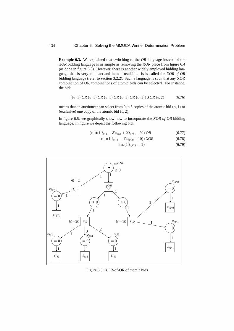
134 Chapter 6. Solving the MMUCA Winner Determination Problem
Example 6.3. We explained that switching to theOR language instead of theXORbidding language is as simple as removing theXORplace from figure 6.4(as done in figure 6.3). However, there is another widely employed bidding lan-guage that is very compact and human readable. Is is called the XOR-of-ORbidding language (refer to section 3.2.2). Such a language is such that any XORcombination of OR combinations of atomic bids can be selected. For instance,the bid:
((a, 1) OR(a, 1) OR(a, 1) OR(a, 1) OR(a, 1)) XOR(b, 2) (6.76)
means that an auctioneer can select from 0 to 5 copies of the atomic bid(a, 1) or(exclusive) one copy of the atomic bid(b, 2).
In figure 6.5, we graphically show how to incorporate theXOR-of-ORbiddinglanguage. In figure we depict the following bid:
(BID(1′tij1 + 3′tij2 + 2′tij3,−20) OR (6.77)
BID(1′tij′1 + 1′tij′2,−10)) XOR (6.78)
BID(1′tij′′1,−2) (6.79)
tij1 tij2 tij3
tij′1
tij′2
= 0
cij1
= 0
cij2
= 0
cij3
= 0
cij′1
= 0
cij′2
tije−20 tij′e−10
1 1 11
13 2
1
1
1
11
•pXOR
i
≥ 0
≥ 0 ≥ 0
tORij′
tij′′1
= 0
cij′′1 tij′′
e−2
1
11
1
11
11
Figure 6.5: XOR-of-OR of atomic bids

6.2. Solving the WDP on Cyclic Mixed Auction Nets 135
The reader can check that this topology allows either firingtij′′ or (exclusive)any of thetij andtij′ if the final contraints represented by inequalities in placesin figure 6.5 are fulfilled.
Notice that in this dissertation we only exploit directly advantages (1) and (3), and weenvisage a promising path for future developments the studyof all the implicationsconnected with advantage (2),(4), and (5). We did not deepeninto considerations con-nected with the study of behavioural and structural properties of the resulting supplychain. Nevertheless, by means of the mapping to WPTNs, we provide all the theoreti-cal and practical tools to deal with such a study.
6.2 Solving the WDP on Cyclic Mixed Auction Nets
So far, we have not been concerned about whether a Mixed Auction Net is cyclic ornot. Is it a reasonable hypothesis considering that a mixed auction net does not containany cycle? The answer is that it depends. One could see a market as a big productioncycle. However, when we consider local production processes, one could think that it ispossible to avoid considering cycles in the topology. Unfortunately, this is not alwaysthe case. Even locally, production cycles are often characterised by cycles. Moreover,we will see that, in our semantics, cycles are required to represent shared resources orresources that can be employed more than once. This is the case, for instance, of a pieceof software or of a tool that is notconsumedbut used. That is, at the end of the supplychain operation the resource is still present, but the operation cannot take place withoutit. With the purpose of clarifying this concept we slightly modify the example of figure6.2.
Example 6.4. We recall that in example 6.2 five bidders participate in a MMUCA. Wemodify bid bid3 introducing the fact that a bidder needs a machineMC to perform thehydrolysis operation. Bidbid3, which stood for a bid on the hydrolysis process fore 8,namely:
bid3 = BID(1′(2′H2O, 1′O2 + 2′H2),−8) (6.80)
turns now into:
bid∗3 = BID(1′(2′H2O + 1′MC, 1′O2 + 2′H2 + 1′MC),−3) (6.81)
Notice that the bidder only requires the MC machine to run thehydrolysis process, andit will release it afterwards. Obviously, we have to includea bid that offers machineMC as well. This is bidbid6:
bid6 = BID(1′(∅, 1′MC),−5) (6.82)
The new configuration of the Mixed Auction Net substitutingbid∗3 with bid3 is shownin figure 6.611.
11In the figure we have omitted all theXOR places, bid transitions, andSCO placesfor the sake of com-prehension.
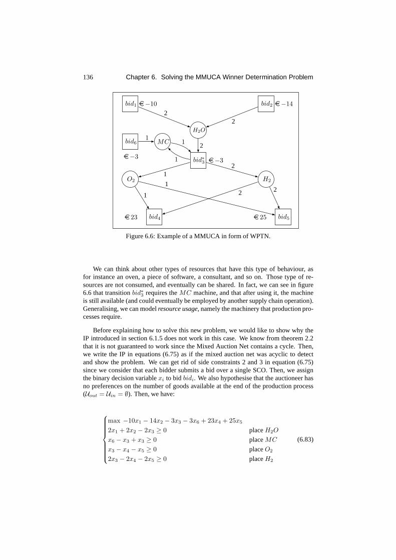
136 Chapter 6. Solving the MMUCA Winner Determination Problem
bid1 e−10 bid2 e−14
bid4e 23 bid5e 25
O2 H2
MC
H2O
bid∗3 e−3
2
12
22
1 21
2
1
1
bid61
e−3
Figure 6.6: Example of a MMUCA in form of WPTN.
We can think about other types of resources that have this type of behaviour, asfor instance an oven, a piece of software, a consultant, and so on. Those type of re-sources are not consumed, and eventually can be shared. In fact, we can see in figure6.6 that transitionbid∗3 requires theMC machine, and that after using it, the machineis still available (and could eventually be employed by another supply chain operation).Generalising, we can modelresource usage, namely the machinery that production pro-cesses require.
Before explaining how to solve this new problem, we would like to show why theIP introduced in section 6.1.5 does not work in this case. We know from theorem 2.2that it is not guaranteed to work since the Mixed Auction Net contains a cycle. Then,we write the IP in equations (6.75) as if the mixed auction netwas acyclic to detectand show the problem. We can get rid of side constraints 2 and 3in equation (6.75)since we consider that each bidder submits a bid over a singleSCO. Then, we assignthe binary decision variablexi to bid bidi. We also hypothesise that the auctioneer hasno preferences on the number of goods available at the end of the production process(Uout = Uin = ∅). Then, we have:
max −10x1 − 14x2 − 3x3 − 3x6 + 23x4 + 25x5
2x1 + 2x2 − 2x3 ≥ 0 placeH2O
x6 − x3 + x3 ≥ 0 placeMC
x3 − x4 − x5 ≥ 0 placeO2
2x3 − 2x4 − 2x5 ≥ 0 placeH2
(6.83)

6.2. Solving the WDP on Cyclic Mixed Auction Nets 137
If we simplify the equations above we obtain:
max −10x1 − 14x2 − 3x3 − 3x6 + 23x4 + 25x5
2x1 + 2x2 − 2x3 ≥ 0 placeH2O
x6 ≥ 0 placeMC
x3 − x4 − x5 ≥ 0 placeO2
(6.84)
the optimal solution isx5 = x3 = x1 = 1 and the remainingxi are0. However, thissolution is not valid! Let us apply the solution. At a first step, SCObid1 is used, provid-ing two units ofH2O to the auctioneer. The following supply chain operation shouldbebid∗3. However, it cannot be used without oneMC, which is currently unavailablebecause we can only obtain it throughbid6. Thus, it is unfeasible to usebid∗3 becausebid6 is not part of the winning bid set.
Then, the solution to the IPis not a valid solution to the MMUCA WDP. Thishappens because the circularity of the net causes the elimination of thex3 variablefrom the equation of placeMC. This is not the only problem. Say that one is luckyand the IP solution matches the solution to the MMUCA WDP, he still should find theordered sequenceof operations. In this case the net is not acyclic and therefore a uniqueorder among transitions cannot be ensured (as stated in corollary 4.1).
We end up this section with a remark that, though neither developed nor formallyproved, can be useful in practice. Say that we compute the IP shown in section 6.1.5for a cyclic mixed auction net (likewise in example 6.4). Saythat we find a solutionrepresented byx∗ (the decision variablesxijk with assigned a value). Say also thatSx∗ is the subnet obtained by the mixed auction net by removing all the transitions notincluded in the solutionx∗ (i.e. removing thetijk such thatxijk = 0). It is intuitive tothink that ifSx∗ is acyclic, then the solution is a valid solution sequence. The sketch ofthe demonstration follows. Recall that a necessary condition for a state to be reachablein a PTN is thatx∗ is a solution to the state equation (see section 2.3.2). However, sincethe hypothesis is that the mixed auction net is cyclic, we cannot guarantee that the stateis reachable. Nevertheless, observe thatx∗ is a solution to the state equation associatedto the subnetSx∗ as well. Then, ifSx∗ is acyclic, the state is reachable in virtue ofcorollary 4.1. Then,x∗ is a valid solution.
Although this observation may seem very powerful, in practise the situation de-scribed above is rather unusual. However, it should be takeninto account.
6.2.1 Modifying the representation
By means of example 6.4 we showed that on cyclic nets the IP defined in section 6.2cannot be applied. In the example we have also shown that the circularity of the net maycause an elimination of some decision variables. This elimination acts so that a checkon the feasibility of a given solution is required. In order to overcome such problem,we modify the IP presented in section 6.2 in such a way that it is possible to check ateach step of the SCO sequence whether enough resources are available to perform theselected SCO. In particular, we modify the way the SCOs are represented.

138 Chapter 6. Solving the MMUCA Winner Determination Problem
The new SCO encoding incorporates some information about the order in whichthe SCOs must be performed. In order to obtain this new representation, we builddirectly upon the definition of WDP (definition 5.10). However, notice that buildingupon the mixed auction net or on the CMWOSP one can obtain similar conclusions.The improved IP model resulting from the new representationis calledDirect IntegerProgramming(DIP) solver.
According to definition 5.10, a solution to the WDP is a mapping Σ from the posi-tions in the solution sequence to the atomic SCOs. Based on this, we define an IP modelwith the following decision variables:xm
ijk ∈ {0, 1} is a binary decision variable thattakes on value 1 if SCOtijk holds positionm in the solution sequence, and 0 otherwise.These variables are the mathematical representation of something similar toΣ. In fact,we can associate to an elementtijk a positionm in a sequence ifxm
ijk = 1. However,we can have someempty positions. The problem is that prevents from having a solutionsuch thatxm
ijk = 0 ∀ijk. This would leave positionm empty. Then, we call a sequencewith empty positionspartial sequence. Obtaining the corresponding sequence from apartial sequence is as easy as removing the empty elements from the partial sequence.Thus, in what follows we will consider thatΣ is a partial sequence, and if we want toretrieve the corresponding sequence we simply remove fromΣ the empty positions.
Σ is obtained from the variablesxmijk in the following way:
Σ(m) =
{
tijk xmijk = 1
⊥ otherwise(6.85)
Obviously we do not know a priori how long the solution sequence will be. Then, werely on the fact that ifδ SCOs are submitted overall by all bidders, the length of thesolution sequence will be at mostδ (there can not be more SCOs in the sequence thanthe ones overall offered).
Observe that employing the binary decision variables above, we can state the fol-lowing relationships12:
OΣ(m)(g) =∑
ijk
xmijkOijk(g) ∀g (6.86)
IΣ(m)(g) =∑
ijk
xmijkIijk(g) ∀g (6.87)
Mm(g) = Mm−1(g) + OΣ(m)(g) − IΣ(m)(g) ∀m, g (6.88)
Mm(g) = Mm−1(g) +∑
ijk
xmijk(Oijk(g) − Iijk(g)) ∀m, g (6.89)
Equation (6.89) can be expanded into the following equationby making explicit its
12We anticipate that the following constraints must be added to ensure thatΣ is afunction:
X
ijk
xmijk ≤ 1

6.2. Solving the WDP on Cyclic Mixed Auction Nets 139
recursive structure:
Mm(g) =
m∑
l=1
∑
ijk
xlijk(Oijk(g) − Iijk(g)) ∀m, g (6.90)
6.2.2 The general IP formulation
We now show how to map the WDP in definition 5.10 into integer programming (IP).Therefore, the issue is to decide for each SCO whether it is selected for the solutionsequence, and if so, to choose its position in the solution sequence. Thus, we define aset of binary decision variablesxm
ijk ∈ {0, 1}, wherexmijk takes on value 1 if the SCO
tijk is selected at them-th position of the solution sequence (tijk = Σ(m)), and 0otherwise. Here and in what follows:
• m always ranges from 1 toδ, the maximum length of the solution sequence;
• i ranges over all bidders;
• for each bidderi, j ranges from 1 to the number of atomic bids submitted byi;
• for each atomic bidj of bidderi, k ranges from 1 to the number of SCO in thatatomic bid;
• g ranges over all goods.
We also introduce several sets of auxiliary binary decisionvariables:
• xijk ∈ N is an integer decision variables that takes on valuew iff transition tijk
is present anywhere in the sequencew times (|Σ−1(tijk)| = w);
• xij ∈ {0, 1} takes on value 1 iff any of the SCOs in thejth atomic bid of bidderiare selected. Equivalently,xij takes on value 1 iff bidBidij is selected.
In what follows, we define the set of constraints that the solution sequence must fulfil:
(1) We enforce the constraints expressed by condition (1) ofdefinition 5.9. Thus,if bid Bidij is selected, all the SCOstijk in that bid must be selected exactlyDij(tijk) times. In other words, if bidBidij is selected, all the SCOs in it mustbe selected with the required multiplicity. Formally,
xij · Dij(tijk) =∑
m
xmijk (∀ijk) (6.91)
(2) We enforce that the atomic bids submitted by each bidder are exclusive (XOR).This amounts to satisfying the following constraints (cf. condition (2) of Defini-tion 5.9):
∑
j
xij ≤ 1 (∀i) (6.92)
Observe that in the case of theORbidding language we simply have to removethis constraint.

140 Chapter 6. Solving the MMUCA Winner Determination Problem
(3) We also impose that at most one SCO is selected at each position of the sequence:∑
ijk
xmijk ≤ 1 (∀m) (6.93)
This equation encodes the hypothesis of no simultaneous firings and enforces thattheΣ built with thexm
ijk is a function, i.e. it does not have two images associatedthe same element (cfr. equation (6.85))
(4) Next, we capture condition (3) of Definition 5.9: enough goods must be availableat stepm to perform the next SCO (cf. equation (5.15)). We recall thatthis mapsto the following condition:
Mm−1(g) ≥ Im(g) ∀g
which is translated, according to equations (6.87) and (6.90), into:
U0(g) +
m−1∑
l=0
∑
ijk
xlijk · [Oijk(g) − Iijk(g)] ≥
∑
ijk
xmijk · Iijk(g) (6.94)
∀g, ∀m
(5) And finally, after having performed all the selected SCOs, the set of goods heldby the auctioneer must be a superset of the final goodsUout (cf. condition (4) ofDefinition 5.9):
Mδ(g) ≥ Uout(g) ∀g
that turns into
U0(g) +
δ∑
m=0
∑
ijk
xmijk · [Oijk(g) − Iijk(g)] ≥ Uout(g) ∀g (6.95)
Now solving the WDP for MMUCAs with XOR-bids amounts to solving the fol-lowing integer program:
max∑
ij
xij · pij subject to constraints (6.91)– (6.95) (6.96)
In table 6.1, we summarise the DIP formulation employing thesame notation as the IPin equation (6.75), with the exception of the symbolIijkg , that stands forIijk(g).
Finally, a valid solution according to definition 5.10 is obtained from the solution ofthe IP by making transitiontijk them-th element of the partial sequenceΣ iff xm
ijk = 1,and then removing the empty positions. In appendix A.2 we present this model encodedin the OPL language (see section 2.1.2 and (Van Hentenryck, 1999)).
Observe that our proposed implementation can easily be amended so as to directlyencode the constraints imposed by language constructs other than the XOR-operator.This would remove the need for translating into the XOR-language first and therebygreatly improve efficiency.

6.2. Solving the WDP on Cyclic Mixed Auction Nets 141
(a) ∀ijk xijk =∑
m
xmijk
(b) ∀ijk xijk = xij · Dij(tijk) ∀ijk
(c) ∀i∑
j
xij ≤ 1
(d) ∀m∑
ijk
xmijk ≤ 1
(e) ∀g uing +
∑
m
∑
ijk
xmijk · aijkg ≥ uout
g
(f) ∀g, ∀m uing +
m−1∑
l=0
∑
ijk
xlijk · aijkg ≥
∑
ijk
xmijk · Iijkg
(g) max∑
ij
xij · pij
Table 6.1: Resume of the IP formulation of solver DIP.
Problem Size
The number of decision variables in the above integer program is of the order ofO(|T | ·δ) (corresponding toxm
ijk). More in details, we create a binary decision variablexij
for each bidBidij ∈ B, for a total of|B| binary decision variables. Then, we create adecision variablexm
ijk for each SCOtijk ∈ T and for each positionm in the solutionsequence, for a total of|T | · ℓ binary decision variables. Assuming, in the general case,that the maximum length of the solution sequence isℓ = δ, then we have|T | · δ =|T | ·
∑
ij |Dij | decision variables. Then, we create a total of
|B| + |T |(1 + δ) ∈ O(|T | · δ)
decision variables. With a similar process, we compute the total number of constraints,that is:
|T | + |L| + δ + |G|δ + |G| ∈ O(|G|δ) (6.97)

142 Chapter 6. Solving the MMUCA Winner Determination Problem
Example 6.5. For the problem presented in figure 6.4, we have the followingdata:
|L| = 1 |B| = 2
|G| = 9 |T | = 5
δ = 8
Then, in the case of the IP in section 6.1.5 the number of decision variables created is7, and the number of constraints is 9+5+1=15. In the case of the IP presented in thissection, we have 45 decision variables and 5+1+8+56+9=79 constraints.
6.3 Computational Complexity
In his master thesis (Ottens, 2007), Ottens provides a detailed proof of the NP-completeness of the decision problem underlying the MMUCA WDP. We briefly recallthe employed argumentation in what follows.
The (decision problem underlying the) WDP for standard combinatorial auctions isknown to be NP-complete, with respect to the number of goods(Rothkopf et al., 1998).NP-hardness can, for instance, be shown by reduction from the well-known SET PACK-ING problem. As our mixed auction model generalises standard combinatorial auctions,winner determination remains NP-hard also here. NP-membership (and thereby NP-completeness) of the problem of checking whether there exists a solution exceeding agiven revenue (for finite bids) follows from the fact that a candidate solution providedby an oracle can always be verified in polynomial time. That is, despite of the gen-eralisations we have introduced, the computational complexity of the WDP does notincrease, at least not with respect to the polynomial hierarchy.
6.4 Conclusions
In this chapter we dealt with the problem of solving the MMUCAWDP, as defined inchapter 5. With this aim, we provided a mapping of the MMUCA WDP to a CMWOSPon the Mixed Auction Net. Some benefits stemed from this mapping. Firstly, sincethe mixed auction net is a WPTN, it provides a very powerful theoretical frameworkfor analysing the MMUCA WDP computational, structural and behavioural proper-ties. Secondly, consequence of the first benefit, we provide an efficient mapping of theMMUCA WDP to ILP for acyclic mixed auction nets. Thirdly, since WPTNs have asso-ciated a very appealing graphical representation, they provide a graphical framework tocompactly represent both the search space and the solutionsassociated to the MMUCAWDP. This is due to the perfect matching between the semantics of transitions and thesemantics of SCOs. We recall that we focus on the computational advantages providedby the mapping to CMWOSP, and leave out for future developments the analysis of thestructural and behavioural properties of the solutions to the MMUCA WDP. However,we remark that the mapping to CMWOSP provides the needed theoretical and practicaltools to perform such analysis.
Next, we show that the hypothesis that the mixed auction net is acyclic sometimesmay not hold. In such a case, the ILP based on the CMWOSP cannotbe employed.

6.4. Conclusions 143
Hence, we provide a general IP solver, theDirect Integer Programming(DIP) solver,that directly builds upon the definition of the MMUCA WDP. This solver allows tosolve the MMUCA WDP on any supply chain network topology. However, it has thedisadvantage to be computationally more costly. In fact, itrequires more decision vari-ables to be encoded.
Notice that the mixed auction net provides a framework toa priori assess the solverto employ, either the CMWOSP-based, if no cycles are presentin the mixed auctionnet, or the DIP otherwise. With this tool at hand, one can build computationally effi-cient MMUCAs. For instance, one approach could be constraining the participants toan MMUCA to bid on sets of SCOs that do not form cycles. This would ensure theabsence of cycles in the correspondingMixed Auction Net, thus allowing the use of theCMWOSP-based solver. However, as motivated by some examples provided in thischapter, sometimes it is not possible to avoid cycles in theMixed Auction Net.
Recent contributions on computationally efficient WDP solvers for different auc-tion types (namely, (Lehmann et al., 2006) for CAs and (Engelet al., 2006) for multi-attribute double auctions) agree on and defend that a careful, formal analysis of thestructure of WDPs can provide guidance for developing efficient winner determina-tion solvers. Along the lines of these works, in the next chapter, we propose an IP forMMUCAs that dramatically improves the computational efficiency of the DIP solver.


Chapter 7
Connected Component-basedSolver
In the previous chapter we presented DIP, an ILP that can solve MMUCA WDPs on anynetwork topology. Then, in section 6.2.2 we showed that DIP requires O(|T |δ) decisionvariables to be represented. This means that the associatedsearch space is very large.In this section we reduce the search space associated the MMUCA WDP.
Recent contributions on computationally efficient WDP solvers for different auctiontypes (namely, (Lehmann et al., 2006) for CAs, (Engel et al.,2006) for multi-attributedouble auctions, as well as our contribution in section 4 forMUCRAtR) agree on anddefend that a careful, formal analysis of the structure of WDPs can provide guidancefor developing efficient winner determination solvers. Along the lines of these works,in this chapter we present a technique to reduce the search space associated to theMMUCA WDP. This will result in an ILP formulation for MMUCA WDPs that dra-matically improves the computational efficiency of the DIP solver presented in section6.2.2.
At this aim, we found our analysis on observing the structureof the WDP that re-sults after establishingdependence relationshipsamong transformations. For instance,in the example ofGrandma & co(depicted in figure 1.1) theBakingSCO potentiallydepends on theMake DoughSCO, since the output provided byMake Doughmay be re-quired to performBaking. The analysis of the WDP based on dependency relationshipshelps design an IP thata priori establisheswhento useeach transformation. There-fore, the search space reduction is achieved by enforcing MMUCA solutions to fulfil atemplate. The template reduces the possible orderings among transformations withoutlosing solutions.
This chapter is organised as follows. In section 7.1 we explain the intuitions under-lying the improvement we propose by means of examples, and inthe remaining sectionswe develop a rigorous description of those intuitions. In section 7.2 we introduce thesolution template allowing a reduction in the search space along with some mathemat-ical tools required in the chapter. In section 7.3 we presenttheConnected ComponentInteger Programming(CCIP) solver, an ILP formulation improving the DIP solver by
145

146 Chapter 7. Connected Component-based Solver
exploiting the solution template. Then, in section 7.4, we prove that the search spacereduction imposed by the solution templates does not cause aloss of solutions. Finally,in section 7.5 we draw some conclusions.
7.1 Motivation and Example
In this chapter we introduce a technique to reduce the searchspace associated to thesolution of MMUCA WDPs. Then, we apply this new representation to encode a newILP solver for MMUCA, the CCIP. CCIP substantially reduces the number of variablesand constraints used by DIP.
The search space reduction is obtained by observing that DIPproduces severalequivalentsolutions. We regard two solutions asequivalentif they select the samebids. As a consequence, equivalent solutions contain the same supply chain operations(SCOs) (even if arranged in different order), and they have associated the same cost. Inwhat follows we provide the rationale to achieve such reduction and to found CCIP.
Example 7.1. Recall from section 5.4.2 that in a MMUCA WDP the input is composedof: (1) the initially available goods (Uin ∈ NG); (2) the finally required goods (Uout ∈NG); and (3) a set of bids in the XOR bidding language (Bidij = (Dij , pij)). Hence,let us consider an MMUCA WDP scenario characterised as follows:
• Uin = ∅ andUout = ∅: no goods are initially available and no goods are requiredat the end of the auction.
• Eight bidders submit the eight bids showed in equations 7.1 to 7.8.
Bid11 = (3′t0 + 1′t1,−3 USD) (7.1)
Bid21 = (2′t2, 9 USD) (7.2)
Bid31 = (1′t3,−2 USD) (7.3)
Bid41 = (1′t4,−1 USD) (7.4)
Bid51 = (1′t5,−8 USD) (7.5)
Bid61 = (2′t6 + 2′t7,−3 USD) (7.6)
Bid71 = (1′t8,−12 USD) (7.7)
Bid81 = (1′t9 + 2′t10,−4 USD) (7.8)
We recall thatBidij = (α′hth, pij) means that bidderi offersαh copies of SCO
th (Dij(th) = k) at pricepij in his j-th bid. For instance, bidBid11 offers ina bundle (combinatorial bid) three units oft0 and one unit oft1 at a price of3USD1. More formally,D11 = {3′t0 + 1′t1}.
Recall from section 5.4.2 thatD = ⊎ijDij is the union of multisets submitted ineach bid. For the bids in equations 7.1 to 7.8, we have:
D = {3′t0 +1′t1 +2′t2 +1′t3 +1′t4 +1′t5 +2′t6 +2′t7 +1′t8 +1′t9 +2′t10} (7.9)
1Recall that the negative sign means that a bidder is willing to be paid.

7.1. Motivation and Example 147
Recall also that the maximum lengthℓ of the solution sequence will be at most equal tothe overall number of atomic SCOs submitted, namely
ℓ = δ =∑
ij
|Dij | = 17
Finally, recall thatT is the set of all the received SCOs (disregarding their multi-plicity).
T = {t0, t1, t2, t3, t4, t5, t6, t7, t8, t9, t10} (7.10)
g2
g3 g4
g5
g6g7
g1
3′t01
1′t1
1
2′t2
1
11′t3
1
1
1′t4 11
1′t5
1
1
2′t6
1
1
2′t7
1
11
1′t81 1
1′t9
1 1
2′t10
11
Figure 7.1: Graphical representation for the SCOs in bids inequations 7.1 to 7.8
In figure 7.1 we graphically represent SCOst1, . . . , t10 contained in the bids ofequations 7.1 to 7.8. The formalism employed in the figure is similar to the one em-ployed in chapter 6. Figure 7.1 represents a Petri Net Structure (PTNS) in which eachtransitions represents a SCO and each place a good. The input/output arcs from/to SCOsdepict the input/output multisets of each SCO. We recall that the arc weights representthe input and output multiplicity of each SCO (for instance,according to figure 7.1, the

148 Chapter 7. Connected Component-based Solver
input and output multisets of SCOt7 are respectivelyIt7 = {g5} andOt7 = {g7, g6}).Notice that in our example every arc has weight1.
Unlike the formalism employed in chapter 6, in the PTNS of figure 7.1 the infor-mation about complementarities among SCOs and the XOR relationships is omitted.Furthermore, we label each SCO with its multiplicity in eachbid. For instance,3′t0means that three units oft0 have been submitted in a bid.
At this point consider that solver DIP solves the WDP with theinput expressed byequations 7.1 to 7.8, and finds the solution sequence in table7.1. The first row in table7.1 represents a position within the solution sequence (them index in variablesxm
ijk
of section 6.2), whereas the second row shows the SCO assigned to the each positionwithin the solution sequence. For instance, the fact that inthe second row and secondcolumn we find SCOt2 means that position2 of the solution sequence is assigned tot2(in DIP this means that in the solutionx2
t2= 1).
Position 1 2 3 4 5 6 7 8 9 10 11 12 13 14 15 16 17 RevenueSequence 1 t0 t2 t1 t0 t4 t0 t2 t3 +3 USD
Table 7.1: Example of solution found by solver DIP.
Thus, according to definition 5.9 of section 5.4.2, the solution of table 7.1 corre-sponds to the following solution sequence:
Σ = 〈t0, t2, t1, t0, t4, t0, t2, t3〉 (7.11)
Notice that the solution sequenceΣ, according to what explained in section 6.2.1, isobtained by removing theempty positionsin Sequence 1of table 7.1.
Accordingly, the winning bids areBid11, Bid21, Bid31, andBid41, and the rev-enue associated to this solution is−3 + 9 − 2 − 1 = 3. As the reader can check, thissolution is valid, since the semantics of the bidding language is fulfilled, and at eachstep of the solution sequence there are enough input goods available to perform thecorresponding SCO. Now consider all the solutions in table 7.2. These solutions areall valid and optimal (they have associated the same revenue) as much as the one intable 7.1. They are simply a rearrangement of the very same solution along differentpositions of the solution sequence, without modifying the relative order among them(i.e. they all represent the sameΣ of equation 7.11).
Position 1 2 3 4 5 6 7 8 9 10 11 12 13 14 15 16 17 RevenueSequence 2 t0 t2 t1 t0 t4 t0 t2 t3 +3 USDSequence 3 t0 t2 t1 t0 t4 t0 t2 t3 +3 USDSequence 4 t0 t2 t1 t0 t4 t0 t2 t3 +3 USDSequence 5 t0 t2 t1 t0 t4 t0 t2 t3 +3 USDSequence 6 t0 t2 t1 t0 t4 t0 t2 t3 +3 USD
Table 7.2: Solutions equivalent to the solution in table 7.1with same relative order.
Now consider the solutions in table 7.3. They are still validsolutions equivalent toSequence 1in table 7.1, though not only the positions assigned to SCOs are different,but also the relative order among them has been altered. Although those solutions

7.1. Motivation and Example 149
correspond to valid solution sequences different from the one in equation 7.11, it iseasy to check that those solutions are still valid. Indeed, at each step of the solutionsequence there are enough inputs to perform the corresponding SCOs. Hence, all theconsidered solutions are Pareto optimal, and equivalent among them.
Position 1 2 3 4 5 6 7 8 9 10 11 12 13 14 15 16 17 RevenueSequence 7 t0 t1 t0 t2 t0 t2 t4 t3 +3 USDSequence 8 t0 t0 t0 t1 t2 t2 t4 t3 +3 USD
Table 7.3: Solutions equivalent to the solutions in table 7.1 with different order.
At this point, the reader is ready to understand what we mean by equivalent solu-tions. Solutions of solver DIP that select the same bids (and thus the same SCOs) haveassociated the same cost. Thus, we hypothesise that they areindistinguishable for anauctioneer.
Notice that, as shown in example 7.1, the search space of solver DIP contains ahuge amount of equivalent solutions. Hence, in order to reduce the complexity of ourproblem, we aim at understanding why all those redundant solutions are found. Asexplained in section 6.2, the IP formulation of solver DIP isfounded on the hypothesisthat a SCO can hold any position within the solution sequence(recall that we createdecision variablesxm
ijk for each positionm and for each SCOtijk ∈ T ), and we set thelength of the solution sequence equal to the overall number of received SCOs, namelyδ. Thus, in principle, each SCO can take one amongδ available positions. This explainswhy all those equivalent solutions are contained in the DIP search space: a large numberof equivalent rearrangements of SCOs within the solution sequence are allowed.
The fact that many equivalent solutions can be found impliesa larger search spacethan needed, and thus an increased computational cost. Suchcomputational cost isreflected in the number of decision variables employed for solver DIP. In the case ofexample 7.1, for instance,t0 has the possibility to take on any of the17 positions of thesolution sequence. Hence, DIP requires17 decision variables fort0. Then, for all theSCOs it requiresδ|T | = 11 ∗ 17 = 187 decision variables. If we manage to reduce thenumber of equivalent solutions contained in the search space, we cut down the numberof decisions, and consequently the search space.
Then, the strategy we follow to reduce the search space consists in limiting thepossible positions each SCO may take on in a solution sequence. In this way the numberof feasible solutions is reduced. Obviously, if we limit thepositions each SCO can takeon we lose solutions as well. The main point here islosing solutions that are equivalentto solutions that in turn are found. For instance, an auctioneer is willing to lose all butone of the solutions in tables 7.1, 7.2, and 7.3 . If at least one is found, we assume thatan auctioneer is not bothered by losing all the other equivalent solutions.
We assume that if two solutions are equivalent, from an auctioneer’s point of vieweliminating one of them from the space of feasible solutionsdoes not constitute a prob-lem. However, given a set of equivalent solutions, the auctioneer needs that at least oneof them is included in the space of feasible solutions.

150 Chapter 7. Connected Component-based Solver
We employ a terminology related to equivalence classes in order to explain thisconcept. It is easy to verify that the relationis equivalent toon the set of DIP solutionsis an equivalence relation (refer to section 2.4.1 for the theory underlying equivalencerelations). In these terms, our goal consists in finding a solution template that:
• reduces the number of equivalent solutions contained in thesearch space, and
• ensures that at least one feasible solution for each equivalence class is found.
That is, we must ensure that no solution class is completely removed from the searchspace. Hereafter, with an abuse of terminology, we say that we lose a solution classwhen we lose a whole equivalence class of solutions.
In what follows we explain how to reduce the search space. We employ a functionthat reduces the possible positions any SCOs can take on in the solution sequence.
Example 7.2. Say that we constraint1 to hold only the first position in a solutionsequence. All the solutions in tables 7.1, 7.2, and 7.3 are still valid if we pusht1 aheadin front of the sequence. For instance, the solution sequences in table 7.3 produces theequivalent solutions represented in table 7.4.
Position 1 2 3 4 5 6 7 8 9 10 11 12 13 14 15 16 17 RevenueSequence 9 t1 t0 t0 t2 t0 t2 t4 t3 +3 USDSequence 10 t1 t0 t0 t0 t2 t2 t4 t3 +3 USD
Table 7.4: Solutions equivalent to the solutions in table 7.3 pushingt1 ahead.
In general, every solution found by DIP to the considered problem can be reorderedinto a solution witht1 in the first position. Then, we pusht2 in the first position of thesolution sequences in table 7.3, and we obtain the sequencesin table 7.5.
Position 1 2 3 4 5 6 7 8 9 10 11 12 13 14 15 16 17 RevenueSequence 11 t2 t0 t0 t2 t0 t1 t4 t3 +3 USDSequence 12 t2 t0 t0 t0 t1 t2 t4 t3 +3 USD
Table 7.5: Solutions equivalent to the solutions in table 7.3 pushingt2 ahead.
None of the sequences in table 7.5 is a valid solution to solver DIP sincet2 cannotoperate without input goods (g2). In this case, placingt2 at the first position is notsafe,since the SCOs that can provide it with input goods are not performed before it.
Then, all the solutions found by solver DIP can be reordered into solutions havingt1 at the first position without losing solution classes. Oppositely, not all the solutionsfound by DIP can be reordered into a solution havingt2 at the first position. Therefore,if we constraint2 to take on the first position, we lose solution classes.
Why it is possible to push aheadt1 and nott2? The reason is thatt2 maydependonother SCOs to be performed. In factt2 may need some inputs that in turn are producedby other SCOs (t0 andt1 in the case oft2). Then, if we want provide a solution templatethat limits the positions that each SCO can hold without causing a loss of solutions, thenwe have to consider those dependencies among SCOs.
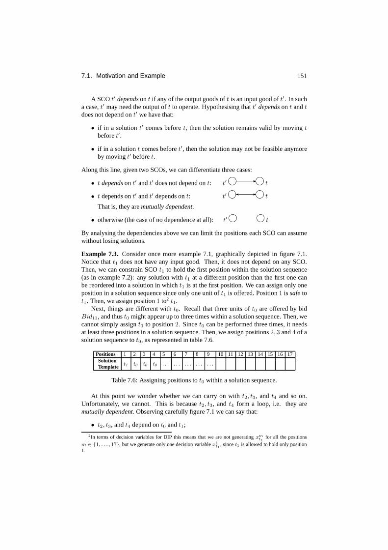
7.1. Motivation and Example 151
A SCOt′ dependson t if any of the output goods oft is an input good oft′. In sucha case,t′ may need the output oft to operate. Hypothesising thatt′ dependson t andtdoes not depend ont′ we have that:
• if in a solutiont′ comes beforet, then the solution remains valid by movingtbeforet′.
• if in a solutiont comes beforet′, then the solution may not be feasible anymoreby movingt′ beforet.
Along this line, given two SCOs, we can differentiate three cases:
• t dependson t′ andt′ does not depend ont: t′ t
• t depends ont′ andt′ depends ont: t′ t
That is, they aremutually dependent.
• otherwise (the case of no dependence at all):t′ t
By analysing the dependencies above we can limit the positions each SCO can assumewithout losing solutions.
Example 7.3. Consider once more example 7.1, graphically depicted in figure 7.1.Notice thatt1 does not have any input good. Then, it does not depend on any SCO.Then, we can constrain SCOt1 to hold the first position within the solution sequence(as in example 7.2): any solution witht1 at a different position than the first one canbe reordered into a solution in whicht1 is at the first position. We can assign only oneposition in a solution sequence since only one unit oft1 is offered. Position1 is safetot1. Then, we assign position 1 to2 t1.
Next, things are different witht0. Recall that three units oft0 are offered by bidBid11, and thust0 might appear up to three times within a solution sequence. Then, wecannot simply assignt0 to position2. Sincet0 can be performed three times, it needsat least three positions in a solution sequence. Then, we assign positions2, 3 and4 of asolution sequence tot0, as represented in table 7.6.
Positions 1 2 3 4 5 6 7 8 9 10 11 12 13 14 15 16 17SolutionTemplate t1 t0 t0 t0 . . . . . . . . . . . . . . .
Table 7.6: Assigning positions tot0 within a solution sequence.
At this point we wonder whether we can carry on witht2, t3, andt4 and so on.Unfortunately, we cannot. This is becauset2, t3, and t4 form a loop, i.e. they aremutually dependent. Observing carefully figure 7.1 we can say that:
• t2, t3, andt4 depend ont0 andt1;
2In terms of decision variables for DIP this means that we are not generatingxmt1
for all the positions
m ∈ {1, . . . , 17}, but we generate only one decision variablex1t1
, sincet1 is allowed to hold only position1.

152 Chapter 7. Connected Component-based Solver
• t2, t3, andt4 do not dependent3 on t5, . . . , t10;
• t2, t3, andt4 are mutually dependent4; and
• t5, . . . , t10 dependends ont2, t3, andt4.
Then, t2, t3, andt4 must come beforet5, . . . , t10 and aftert0 and t1. However, wecannot establish an order among them since they are mutuallydependent. Thus, wemust consider all their possible orderings. For instance, we can assign tot2, t3, andt4positions5, 6, 7, and8 (since two units oft2 are available, we must assign two positionsto t2). Table 7.7 outlines atemplateof a solution built in this way.
Positions 1 2 3 4 5 6 7 8 9 10 11 12 13 14 15 16 17
SolutionTemplate
t1 t0 t0 t0
t2t3t4
t2t3t4
t2t3t4
t2t3t4
t5 t9 t10 t10t6t7
t6t7
t6t7
t6t7
t8
#Variables 1 1 1 1 3 3 3 3 1 1 1 1 2 2 2 2 1
Table 7.7: Positions within the solution sequence assigneda-priori to SCOs.
Notice that we now need a decision variable for each of the elements in table 7.7 (asexpressed in the last row of the table). As tot2, t3, andt4, the possible choices can beencoded by the following variables:
{x5t2
, x6t2
, x7t2
, x8t2
, x5t3
, x6t3
, x7t3
, x8t3
, x5t4
, x6t4
, x7t4
, x8t4} (7.12)
wherex5t2
= 1 means thatt2 is performed at the5-th position.Then, the total number of decision variables required to represent the problem
amounts to:
1 + 1 + 1 + 1 + 3 · 4 + 1 + 1 + 1 + 1 + 2 · 4 + 1 = 29 (7.13)
In contrast, table 7.8 illustrates the assignment of positions as required by DIP. DIP em-ploys 11 ∗ 17 = 187 variables overall. Therefore, the difference when constrainingSCOs to limited number of positions is very significant (29 versus187 in the example).
To conclude, we have to detect the dependencies present in the structure induced bythe SCOs and apply the process described above: we assign an a-priori limited numberof positions within the solution sequence to each SCO (or group of SCOs).
In what follows, we formally analyse how we can extend the intuitions above to thegeneral case in order to yield a new IP, the so called CCIP, by relying on the notion ofdependence among transformations, and using it to constrain the positions at which atransformation can be used.
3No matter the ordering amongt2, t3, andt4, we can always assign to them positions beforet5 or t9without losing solutions.
4Notice thatt2, t3, andt4 lie on a cycle in the net. For this reason, each of them could contribute toprovide goods to the inputs of the other.
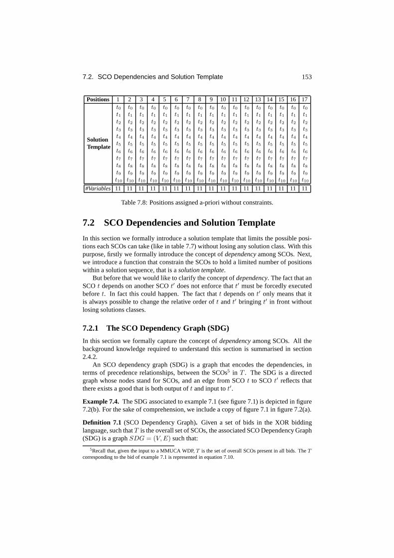
7.2. SCO Dependencies and Solution Template 153
Positions 1 2 3 4 5 6 7 8 9 10 11 12 13 14 15 16 17
SolutionTemplate
t0t1t2t3t4t5t6t7t8t9t10
t0t1t2t3t4t5t6t7t8t9t10
t0t1t2t3t4t5t6t7t8t9t10
t0t1t2t3t4t5t6t7t8t9t10
t0t1t2t3t4t5t6t7t8t9t10
t0t1t2t3t4t5t6t7t8t9t10
t0t1t2t3t4t5t6t7t8t9t10
t0t1t2t3t4t5t6t7t8t9t10
t0t1t2t3t4t5t6t7t8t9t10
t0t1t2t3t4t5t6t7t8t9t10
t0t1t2t3t4t5t6t7t8t9t10
t0t1t2t3t4t5t6t7t8t9t10
t0t1t2t3t4t5t6t7t8t9t10
t0t1t2t3t4t5t6t7t8t9t10
t0t1t2t3t4t5t6t7t8t9t10
t0t1t2t3t4t5t6t7t8t9t10
t0t1t2t3t4t5t6t7t8t9t10
#Variables 11 11 11 11 11 11 11 11 11 11 11 11 11 11 11 11 11
Table 7.8: Positions assigned a-priori without constraints.
7.2 SCO Dependencies and Solution Template
In this section we formally introduce a solution template that limits the possible posi-tions each SCOs can take (like in table 7.7) without losing any solution class. With thispurpose, firstly we formally introduce the concept ofdependencyamong SCOs. Next,we introduce a function that constrain the SCOs to hold a limited number of positionswithin a solution sequence, that is asolution template.
But before that we would like to clarify the concept ofdependency. The fact that anSCOt depends on another SCOt′ does not enforce thatt′ must be forcedly executedbeforet. In fact this could happen. The fact thatt depends ont′ only means that itis always possible to change the relative order oft andt′ bringing t′ in front withoutlosing solutions classes.
7.2.1 The SCO Dependency Graph (SDG)
In this section we formally capture the concept ofdependencyamong SCOs. All thebackground knowledge required to understand this section is summarised in section2.4.2.
An SCO dependency graph (SDG) is a graph that encodes the dependencies, interms of precedence relationships, between the SCOs5 in T . The SDG is a directedgraph whose nodes stand for SCOs, and an edge from SCOt to SCOt′ reflects thatthere exists a good that is both output oft and input tot′.
Example 7.4. The SDG associated to example 7.1 (see figure 7.1) is depictedin figure7.2(b). For the sake of comprehension, we include a copy of figure 7.1 in figure 7.2(a).
Definition 7.1 (SCO Dependency Graph). Given a set of bids in the XOR biddinglanguage, such thatT is the overall set of SCOs, the associated SCO Dependency Graph(SDG) is a graphSDG = (V, E) such that:
5Recall that, given the input to a MMUCA WDP,T is the set of overall SCOs present in all bids. TheT
corresponding to the bid of example 7.1 is represented in equation 7.10.

154 Chapter 7. Connected Component-based Solver
• Each SCO is a vertex:V = T ,
• A directed arc connects two SCOst and t′ iff there exists a good that is bothoutput oft and input tot′. More formally,
(t, t′) ∈ E iff Ot ∩ It′ 6= ∅
An SDG may or may not contain cycles. However, we have to assume that the graphis cyclic in the general case. As explained in section 2.4.3,a (cyclic) graph defines apreorder. over T . We denote this preorder as a pair(T, .). The semantics of thepreorder is thatt . t′ iff a path exists betweent andt′. As illustrated in section 2.4.3,a preorder allows the existence of pairs(t, t′) such thatt . t′ andt′ . t.
Example 7.5. In the order defined by the graph in figure 7.2(b) we have thatt1 . t5and t2 . t8. However, considering thatt2 . t3 and t3 . t2, t2 and t3 cannot beordered among them.
Figures 7.2 (a) and (b) depict the PTN structure representing the SCOs of example7.1 along with the corresponding SDG. We recall from chapter2 that, given a setTequipped with a preorder., we can define an equivalence relation∼ onT as follows:
t ∼ t′ iff t . t′ andt′ . t (7.14)
Example 7.6. Regarding the example of figure 7.2(b), the equivalence classes are:
[t0] = {t0} (7.15)
[t1] = {t1} (7.16)
[t2] = {t2, t3, t4} (7.17)
[t5] = {t5} (7.18)
[t6] = {t6, t7} (7.19)
[t8] = {t8} (7.20)
[t9] = {t9} (7.21)
[t10] = {t10} (7.22)
(7.23)
Recall also that it is possible to define a strict partial order over the quotient set(T/∼,≺) such that:
[t] ≺ [t′] iff t . t′ andt 6. t′ (7.24)
Equivalently, we define a strict order on the setT (T,≺) such that:
t ≺ t′ iff [t] ≺ [t′]
Example 7.7. As to the example in figure 7.2(b),[t2] ≺ [t5] (t2 ≺ t5) since there existsa simple path fromt2 to t5 (〈t2, t5〉)6. However[t2] ≺ [t4] does not hold since, althougha simple path exists fromt2 to t4 (〈t2, t4〉), we have thatt2 ∼ t4. In fact there are cycles(〈t2, t4, t3, t2〉).
6Recall that according to the notation employed in section 2.4.2 a path in a graph is noted as〈v1, . . . , vn〉,where thevi are the nodes belonging to the path.

7.2. SCO Dependencies and Solution Template 155
g2
g3 g4
g5
g6g7
g1
t0
t1
t2t3
t4
t5
t6 t7
t8
t9
t10
t2
t4t5 t9
t3
t6
t7
t8
t0 t1
t10
(a) A PTNS representing SCOs (b) SDG
scc234
scc67
scc0 scc1
scc9scc5
scc8
scc10
t2
t4 t9t5
t3
t6
t7
t8
t0 t1
t10
scc0
scc234
scc9 scc5
scc1
scc10 scc67
scc8
(c) SCCs of the SDG (d) The strict order
Figure 7.2: A PTN structure, the corresponding SDG, SCC, andOrder Relation.
Then, we are now ready to formally define the concept ofdependence. We recallthat two SCOst, t′ can be such that: (1)t depends ont′ andt′ does not depend ont;or (3) t andt′ are mutually dependent; or (4)t andt′ are not dependent on one another.More formally, we can distinguish the following three cases:
(1) t ≺ t′: t dependson t′. A one-way directed path betweent and t′ exists inthe SDG. Then, all the SCOs along the path connectingt to t′ can contribute toincrease the input goods oft′. Then,t′ dependson their execution. For instance,in example 7.7, we have thatt5 depends ont2. Therefore, pushingt ahead oft′

156 Chapter 7. Connected Component-based Solver
in a solution sequence does not cause a loss of solution classes.
(2) t′ ∼ t: t andt′ aremutually dependent. There exist both a simple path fromt tot′ and another one fromt′ to t. Therefore, they lie on a simple cycle of the SDG.For instance, in figure 7.2(b), we have thatt2 ∼ t4. Obviously, we cannot orderthem since the circularity of the relationship implies thatthey depend on eachother. Then, we may risk to lose some solution class if we change their relativeorder in a solution sequence.
(3) t 6. t′ andt′ 6. t: no path exists betweent andt′. The relative positions oftandt′ within the solution sequence does not affect the feasibility of the solutionin any case. Then, it does not matter the relative order oft andt′ in the solutionsequence, and it can be changed arbitrarily.
In what follows we present three examples referring to the three items in the list above.
Example 7.8(Dependence). In example 7.2 we were able to movet1 in the first po-sition of the solution sequence without losing solutions, whereas we could not do thesame fort2. This happens sincet1 does not depend on any SCO (∄t such thatt ≺ t′),whereast2 depends ont1 (t1 ≺ t2) andt0 (t0 ≺ t2). Then,t1 andt0 must hold posi-tions previous tot2. This is why in the solution template in table 7.7,t2 comes aftert1andt0.
Example 7.9(Mutual Dependence). In example 7.3, we saw that in the case oft2, t3,andt4 we could not assign to each of these SCOs only one place in the solution se-quence. In fact, we have thatt2 ∼ t3 ∼ t4. Then, in order to consider all the possibleorderings among them, we assigned to them positions5, 6, 7, and8 in the solution tem-plate of table 7.7.
Example 7.10(Independence). In example 7.2 we were able to movet1 in the firstposition of the solution sequence without losing solutions. The reader can check thatequivalentlyt0 can be brought to the first position without affecting the validity of thesolution. Thus, the solution template of table 7.7 can be modified by switching thepositions oft0 andt1 as shown in table 7.9.
Positions 1 2 3 4 5 6 7 8 9 10 11 12 13 14 15 16 17
SolutionTemplate
t0 t0 t0 t1
t2t3t4
t2t3t4
t2t3t4
t2t3t4
t5 t9 t10 t10t6t7
t6t7
t6t7
t6t7
t8
Table 7.9: Interchanging the positions oft1 andt0.
Hence, while we can a-priori establish an order among SCOs belonging to differentequivalence classes, for SCOs within the same equivalence class we cannot since theyare mutually dependent. As to the case of SCOs, we can chose any ordering.

7.2. SCO Dependencies and Solution Template 157
7.2.2 Computing the equivalence classes
As shown in section 2.4, the definition of Strongly ConnectedComponent (SCC) ingraph theory coincides with the notion of equivalence classwe defined above. The verygood news is that there exists an algorithm that can find the SCCs of a graph(V, E) inpolynomial time (Θ(V + E)), as explained in (Cormen, 2001). The fact that we haveavailable this algorithm significantly simplifies the first of our subproblems, that is theproblem of finding an execution order among SCOs. In fact, once obtained the stronglyconnected components, enforcing a suitable ordering amongthem amounts to buildinga solution template.
Henceforth, we will refer indifferently to equivalence classes or SCCs.
Example 7.11.The strongly connected components of the graph in figure 7.2(b) are:
scc0 = {t0} = [t0] scc67 = {t6, t7} = [t6]
scc1 = {t1} = [t1] scc8 = {t8} = [t8]
scc234 = {t2, t3, t4} = [t2] scc9 = {t9} = [t9]
scc5 = {t5} = [t5] scc10 = {t10} = [t10]
They are graphically depicted in figure 7.2(c). As mentionedin section 2.4, it is alsopossible to define a strict order among equivalence classes (SCCs), graphically depictedin figure 7.2(d).
7.2.3 Order Enforcing Function
We mentioned at the beginning of this section that our aim is to build atemplatethatallows us to a-priori limit the set of positions that each SCOcan hold within a solutionsequence in such a way that no solution class is lost. As illustrated by the template intable 7.7, there is a link between the dependencies among SCOs and their relative order.Most precisely, a solution template must comply with the strict order stemming fromdependencies. Next, we provide a formal definition of solution template, the so-calledD-bounded Order Enforcing Function.
Definition 7.2 (D-bounded Order Enforcing Function). Given a strict order(T/∼,≺)and a multi-setD ∈ NT , aD-bounded Order Enforcing FunctionS : {1, . . . , |D|} →T/∼ is a sequence of equivalence classes satisfying the following constraints:
S(i) ≺ S(j) ⇒ i < j (7.25)
|S−1([t])| =∑
t′∈[t]
D(t′) ∀[t] ∈ T/∼ (7.26)
Where|S−1([t])| is the number of times the equivalence class[t] appears in the se-quenceS. Henceforth,S will denote aD-bounded order enforcing function for(T/∼,≺).
Equation 7.25 guarantees that all the position assigned to the equivalence classesare in increasing order with respect to(T/∼,≺). This means that if[t] comes before

158 Chapter 7. Connected Component-based Solver
[t′] according to(T/∼,≺), then[t] comes before[t′] in S. Equation 7.26 ensures thatenough positions inS are available to contain all the SCOs inD with their multiplicity.For instance, if three units oft0 are offered, it means that up to three copies oft0may be present in the solution sequence. Then, three positions must be assigned tot0 in S. Notice that there is no overlapping among the positions assigned to differentequivalence classes in virtue of equation 7.25.
Example 7.12. If D is the multi-set of the overall SCOs received in the MMUCA ofexample 7.1. We define aD-bounded enforcing functionS as follows:
S(1) = [t1]; S(2) = [t0];
S(3) = [t0]; S(4) = [t0];
S(5) = [t2]; S(6) = [t2];
S(7) = [t2]; S(8) = [t2];
S(9) = [t5]; S(10) = [t9];
S(11) = [t10]; S(12) = [t10];
S(13) = [t6]; S(14) = [t6];
S(15) = [t6]; S(16) = [t6];
S(17) = [t8];
Departing from solution template in table 7.7 we can represent functionS as shownin table 7.10. The solution template readily leads to the mapping in table 7.10 bysubstituting each set of elements for the equivalence classit belongs to. For instance{t2, t3, t4} for [t2] and{t6, t7} for [t6].
Positions 1 2 3 4 5 6 7 8 . . .
Equiv. classes [t1 ] [t0 ] [t0 ] [t0 ] [t2 ] [t2 ] [t2 ] [t2 ] . . .
. . . 9 10 11 12 13 14 15 16 17
. . . [t5 ] [t9 ] [t10 ] [t10 ] [t6 ] [t6 ] [t6 ] [t6 ] [t8 ]
Table 7.10:D-bounded enforcing function for example 7.1.
We employS−1 to indicate the inverse of an enforcing functionS. S−1([t]) indi-cates the set of integers (positions) that map to the equivalence class[t] via S. Moreformally:
S−1([t]) = {m ∈ {1, . . . , |D|} | S(m) = [t]}
Example 7.13.Regarding example 7.12,
S−1([t6]) = S−1([t7]) = {13, 14, 15, 16}
In what follows, we show that it is always possible to build atleast one solutiontemplate. We prove this by construction. This result is fundamental to our purposessince theS function is employed to encode our problem.

7.2. SCO Dependencies and Solution Template 159
Lemma 7.1. Given a strict order(T/∼,≺) and a multi-setD ∈ NT such that∀t ∈T D(t) ≥ 1, at least aD-bounded order enforcing functionS exists.
Proof of lemma 7.1 Let (q1, q2, ..., qk), wherek = |T/∼|, be an ordering of theelements ofT/∼ satisfying≺. Then, we buildS as follows:
S(1) = q1 S(2) = q1 . . . S(λ1) = q1
S(λ1 + 1) = q2 S(λ1 + 2) = q2 . . . S(λ1 + λ2) = q2
. . . . . . . . . . . .
S(∑k−1
l=1 λl + 1) = qk S(∑k−1
l=1 λl + 2) = qk . . . S(∑k−1
l=1 λl + λk) = qk
whereλi =∑
t∈qiD(t) Notice thatS satisfies the constraints specified by equations
7.25 and 7.26.
Notice that this proof also explains how to practically build a solution templategiven the SCCs.
S is thus a function that assigns positions within a sequence to set of SCOs. Themain property ofS is that every solution that DIP finds can be reordered into anequiva-lentandfeasiblesolution that fulfils the solution templateS. In order to formally definethe concept offulfilment, we have to introduce some notation. In fact, we need to link asolution to DIP to the solution templateS. We begin by introducing partial sequences,a generalisation of the concept of sequence that captures the formal representation of asolution to solver DIP (see table 7.1).
7.2.4 Partial Sequences
We begin by recalling the definition of sequence.
Definition 7.3 (Sequence). A Sequenceover a non-empty finite setT is a functionK : [1, n] → T , with n ∈ N.
Notice that in table 7.1 we represented a solution as a mapping from positions withina sequence to SCOs. In what follows we illustrate the conceptof partial sequence,which intuitively is a sequence with “holes”, meaning that there could be some posi-tions of the sequence that areempty. This notion will be employed to formally capturesolution sequences like the ones in tables 7.1, 7.2, and 7.3.
Definition 7.4 (Partial Sequence). A Partial Sequenceover a non-empty finite setT isa partial functionK : [1, n] → T , with n ∈ N.
The fact the function ispartial implies that some integers may have no image,representing the holes in the sequence.
From now on, we will employ the following notation:
(1) |K| the length of the sequence. Henceforth, we will assume|K| = n;
(2) K−1 : T → 2[1,n] is a partial injective function such thatm ∈ K−1(t) iffK(m) = t (inverse function);
(3) |K−1(t)| is the number of timest appears in sequenceK;

160 Chapter 7. Connected Component-based Solver
(4) Given a multi-setD : T → N, we will note asD(t) the multiplicity of t in D;
(5) Dom(K) is the subset of[1, n] that admits an image viaK (domain);
(6) Im(K) = {t ∈ T | K(m) = t for somem ∈ [1, n]} (image)
Example 7.14.The partial sequence representing the solution sequence intable 7.1 is:
K(1) = t0
K(2) = t2
K(5) = t1
K(6) = t0
K(7) = t4
K(8) = t0
K(9) = t2
K(14) = t3
Obviously, a solution sequence can not contain more SCOs than the ones submittedin bids overall. Then, we further refine the representation of solutions by limiting thenumber of times each SCO can appear within a partial sequence.
Definition 7.5 (D-bounded Partial Sequence). Given apartial sequenceK over a setT and a multi-setD ∈ NT , we say thatK is D-bounded if:
|K−1(t)| ≤ D(t) ∀t ∈ Im(K) (7.27)
Example 7.15.The partial function defined in example 7.14 is bounded by themulti-setD in equation 7.9:
D = {t0, t0, t0, t1, t2, t2, t3, t4, t5, t6, t6, t7, t7, t8, t9, t10, t10}
this happens since:
(|K−1(t0)| = 3 andD(t0) = 3
)implies|K−1(t0)| ≤ D(t0) (7.28)
. . . . . . (7.29)
and a similar equation applies to all the other elements inIm(K).
Notice that the multi-setD = ⊎ijDij associated to an MMUCA bounds all of itssolutions, as state in the following observation.
Remark7.1. Every solution to an MMUCA is aD-bounded partial sequence.
Now that we have all the formal tools to describe a solution, we can define when asolutionfulfils a solution templateS (order enforcing function). This is a central pointand leads us to the definition ofS-fulfilment:

7.3. The improved IP formulation 161
Definition 7.6 (S-fulfilment). Given aD-bounded partial sequenceK and aD-boundedorder enforcing functionS, we say thatK fulfils S iff:
∀i ∈ dom(K) K(i) ∈ S(i) (7.30)
This means that a solutionK complies with a solution template if each SCO inKtakes on a positionallowedby S.
Example 7.16.COnsider table 7.11
• the partial sequenceK in does not fulfil the order enforcing function (solutiontemplate)S, sinceK(1) = t2 andS(1) = [t1], but t2 6∈ [t1];
• the partial sequenceK ′ fulfils S.
In table the highlighted SCOs do not hold the positions enforced by the solution tem-plate.
Positions 1 2 3 4 5 6 7 8 9 10 11 12 13 14 15 16 17
(S) SolutionTemplate
t1 t0 t0 t0
t2t3t4
t2t3t4
t2t3t4
t2t3t4
t5 t9 t10 t10t6t7
t6t7
t6t7
t6t7
t8
K t0 t2 t1 t0 t4 t0 t2 t3
K′t1 t0 t0 t0 t2 t4 t2 t3
Table 7.11: Partial sequence fulfilling (K ′) and not fulfilling (K ′) S in table 7.10.
Then, now we can explain why the solution template represented byS is of centralimportance. We will formally prove in section 7.4 that each partial sequence, solutionto the MMUCA WDP, can be reordered into anequivalentand feasiblesolution thatfulfils S. Consequently, if we limit the search space so thatonly the solutions fulfillingS are included, we guarantee that no solution class is lost. Therefore, we achieve whatwe intended, obtaining a space search reduction without sacrificing solution classes.
In the next section we show how to apply an ordering enforcingfunction to ILP.We will present a new solver for the MMUCA WDP, that employs considerably lessdecision variables than DIP by exploitingS.
7.3 The improved IP formulation
The aim of this section is to introduce a new IP that improves solver DIP. We callthe improved solver, described in the remaining of this section, solver CCIP. The ideaunderlying the improvement of solver DIP is to consider as possible solutions onlypartial sequences fulfilling aD-bounded order enforcing functionS and excluding allother solutions. With this purpose, we employ the order enforcing function introducedin definition 7.2.

162 Chapter 7. Connected Component-based Solver
In section 7.3.1, we introduce a preliminary version of the IP formulation of solverCCIP. In section 7.3.2 we introduce a further simplificationthat allows to eliminatepart of the constraints. In section 7.3.3 we show that CCIP turns into a CMWOSPsolver when the Mixed Auction Net is acyclic. Finally, in section 7.3.4 we show thatCCIP turns into the DIP solver when the SDG is connected.
7.3.1 The Model
As usual, the input to the MMUCA WDP is a set of bidsBidij , each one over a multi-setDij along with some pricepij . D =
⋃
ij Dij is the multi-set of all the submittedSCOs. Then, the maximum length of the solution sequence isδ = |D|.
According to remark 7.1, a partial sequence representing a solution to the WDP isalways bounded byD, since the partial sequence will at most contain all the submittedSCOs. Then, we consider aD-bounded order enforcing functionS. The associatedorder relation(T/∼,≺) is the one defined by the SDG graph onT .
In solver DIP we employed binary decision variablexmijk taking on value 1 iff SCO
tijk is selected at them-th position within the solution sequence. In the case of DIP,m ranges in all the positions of the solution sequence (m ∈ [1, δ]). However, now wecan assign a limited number of positions to each SCO viaS. If we want to allow asfeasible solutions only partial sequences fulfillingS, we only create decision variablesfor the positions each SCO can hold. More precisely we createdecision variablesxm
ijk
for all m ∈ S−1([tijk]). By means of this operation we manage to drastically reducethe search space.
Next, analogously to section 6.2, we employ the following auxiliary decision vari-ables. Firstly,xijk is an integer variable that represents the number of positions thatSCOtijk holds in the solution sequence. Secondly,xij is a binary decision variablestaking on value one if bidBidij is selected and 0 otherwise. Then, we impose thefollowing constraints.
(1) We obtain the number of positions that SCOtijk holds in the solution sequence(xijk) by summing upxm
ijk over all the positionsm assigned to[tijk ]:
xijk =∑
m∈S−1([tijk])
xmijk ∀ijk (7.31)
Example 7.17. Regarding example 7.1 we have:
xt2 = x5t2
+ x6t2
+ x7t2
+ x8t2
(7.32)
andxt0 = x2
t0+ x3
t0+ x4
t0(7.33)
and so on.
(2) We are interested in that at most one SCO can hold each position. Consequently,we impose that:
∑
tijk∈S(m)
xmijk ≤ 1 ∀m (7.34)

7.3. The improved IP formulation 163
Notice that the sum is only over the SCOs of a single equivalence class. Theseconstraints enforce that the solution is a partial sequence. Without such a con-straint we could have more than one SCO assigned to the same position of thesequence.
Example 7.18. Following example 7.1, at step 5 (m = 5) the following con-straints hold:
x5t2
+ x5t3
+ x5t4
≤ 1 (7.35)
(3) We need decision variables controlling if a given bid hasbeen selected. As weknow, the semantics of a bid implies that selecting at least one SCO within abid implies selecting all the SCOs within the same bid with the correspondingmultiplicity. That is:
xijk = xij · Dij(tijk) ∀ijk (7.36)
Example 7.19. For SCOt0 in bid Bid11 of the MMUCA of example 7.1 wehave:
xt0 = x11 · 3 (7.37)
and so on.
(4) We impose that the XOR semantics of a bid is fulfilled, i.e.at most one bid perbidder can be selected: ∑
j
xij ≤ 1 ∀i (7.38)
(5) We need to encode the constraint enforcing that each SCO selected is enabled atany step of the solution sequence.
U0(g) +
m−1∑
l=0
∑
tijk∈S(l)
xlijk · [Oijk(g) − Iijk(g)] ≥
∑
tijk∈S(m)
xmijk · Iijk(g)
(7.39)
∀g ∈ G, ∀m ∈ [1, δ]
(6) We express the constraint enforcing that the goods available to the auctioneer atthe end of the solution sequence is at leastUout:
U0(g) +
ℓ∑
m=0
∑
tijk∈S(m)
xmijk · [Oijk(g)−Iijk(g)] ≥ Uout(g) ∀g ∈ G (7.40)
In table 7.12 we summarise the CCIP ILP formulation.Finally, solving the MMUCA WDP is equivalent to optimise theobjective function:
max∑
ij
xij · pij (7.41)
subject to constraints (a-f) in table 7.12.

164 Chapter 7. Connected Component-based Solver
(a) ∀ijk xijk =∑
m∈S−1([tijk ])
xmijk
(b) ∀ijk xijk = xij · Dij(tijk) ∀ijk
(c) ∀i∑
j
xij ≤ 1
(d) ∀m∑
tijk∈S(m)
xmijk ≤ 1
(e) ∀g ∈ G U0(g) +ℓ∑
m=0
∑
tijk∈S(m)
xmijk · [Oijk(g) − Iijk(g)] ≥ Uout(g)
∀g ∈ G U0(g) +
m−1∑
l=0
∑
tijk∈S(l)
xlijk · [Oijk(g) − Iijk(g)] ≥
(f) ∀m ∈ [1, δ]∑
tijk∈S(m)
xmijk · Iijk(g)
(g) max∑
ij
xij · pij
Table 7.12: Resume of the IP formulation of solver CCIP.
7.3.2 Eliminating some Equations
There is a further simplification that we can add. Not only we can reduce the numberof variables, but we are also able to eliminate some redundant constraints. It followsfrom some considerations on the IP structure that we can remove some constraintsfrom solver CCIP because redundant. In what follows we provide the correspondingintuitions.
Equation (7.39) ensures that enough goods are present to perform the selected SCOsat each step of the solution sequence. It must be applied at each step of the solution

7.3. The improved IP formulation 165
sequence.
U0(g) +m−1∑
l=0
∑
tijk∈S(l)
xlijk · [Oijk(g) − Iijk(g)] ≥
∑
tijk∈S(m)
xmijk · Iijk(g) (7.42)
∀g ∈ G, ∀m ∈ [1, δ]
Equation (7.40) states that at the end of the sequence at least Uout goods are availableto the auctioneer.
U0(g) +
ℓ∑
m=0
∑
tijk∈S(m)
xmijk · [Oijk(g) − Iijk(g)] ≥ Uout(g) ∀g ∈ G (7.43)
The application of the two constraints above plus the fact thatS limits the possibleposition assignments makes some of those constraints redundant. In particular, we canget rid of constraint 7.42 at each stepm if the group of SCO assigned to stepm viaS does not belong to any cycle of the graph. The following example will clarify thestatement.
Example 7.20. Consider the MMUCA WDP presented in example 7.1. In particular,we will focus on the equations regarding goodg4 just before the firing oft5. Then,considering that the only SCOs that can add or remove tokens to g4 are{t2, t4, t5, t9},equation 7.43 becomes7:
xt2 − xt4 − xt5 − xt9 ≥ 0 (7.46)
Notice that thextiin in equation 7.46 are integer, not binary variables. Now we
consider equation 7.42 at step9 and for goodg4. According to table 7.7, SCOt5 isassigned to position9. Then, equation 7.42 becomes8:
xt2 − xt4 ≥ xt5 (7.49)
7Equation 7.43 can be rewritten as
0 +
ℓX
l=0
X
t∈{t2,t4,t5,t9}
xlt · [Ot(g4) − It(g4)] ≥ 0 (7.44)
that can be rewritten as0 +
X
t∈{t2,t4,t5,t9}
xt · [Ot(g4) − It(g4)] ≥ 0 (7.45)
sincext =Pℓ
l=0 xlt (equation 6.91). Expanding equation 7.45, we obtain 7.46.
8Equation 7.42 can be rewritten as:
0 +8
X
l=0
X
t∈T
xlt · [Ot(g4) − It(g4)] ≥ x9
t5· It5 (g4) (7.47)
Once again, since the only SCOs that can add or remove tokens to g4 are{t2, t4, t5, t9} and their assignedpositions in table 7.7 are{5, 6, 7, 8, 9, 10}, equation 7.47 becomes:
0 +X
l∈{5,6,7,8}
X
t∈{t2,t4}
xlt · [Ot(g4) − It(g4)] ≥ x9
t5· It5(g4) (7.48)
The reader can check that expanding this expression we obtain equation 7.49.

166 Chapter 7. Connected Component-based Solver
Notice that equation (7.49) is automatically satisfied if equation (7.46) is fulfilled. Then,equation 7.49 is redundant, and we can get rid of it.
Example 7.20 above shows an important properties of our model. This propertyis not very intuitive because it depends on the equations andon their relationships.Anyway, as we mentioned above, this property does not hold ifthe SCO lies on asimple cycle or on a self-loop of the SDG. A counter example will clarify this sentence.
Example 7.21. We consider again example 7.1, but in this case we focus on theequa-tions for goodg1. Notice that a a self-loop is present ont10. This self-loop prevents toapply the same reasoning of example 7.20. First, we write theequivalent of equation7.46 and we obtain:
xt9 + xt10 − xt10 ≥ 0 =⇒ xt9 ≥ 0 (7.50)
Next, we consider equation 7.42 at step11. We obtain:
xt9 − xt10 ≥ 0 (7.51)
It is easy too see that equation 7.50 does not imply equation 7.51. Then, we cannot getrid of equation 7.51.
Intuitively, equation 7.43 is aglobal condition enforcing that at the end of the se-quence the global input-output balance at each good of the net in figure 7.1 is positive.On the other hand, equation 7.42 islocal to each step, and enforces that enough inputgoods are available at each step.
As showed by example 7.21, we have to check constraint 7.42 only when the SCOsassigned to positionm belong to a cycle. Notice that by definition each time an equiv-alence class containsn > 1 SCOs, each SCO in the equivalence class belongs to asimple cycle of lengthn.
Example 7.22. (1) t10 in figure 7.2(a) has goodg1 both as input and output. Then itbelongs to a self-loop (〈t10, t10〉). (2) t2 belongs to the simple cycle〈t2, t4, t3, t2〉. (3)t1 does not belong to any cycle.
To conclude, with respect to the encoding of solver CCIP presented in section 7.3.1,we can get rid of a set of inequations. Thus, besides reducingthe number of variables,we decrements the number of constraints of solver DIP.
Employing the terminology introduced in section 7.3.2, we can say that equation7.39 must be added only if the SCOs assigned to stepm by S belong to a simple cycle.Then, definingLF as:
LF = {m ∈ {1, . . . ℓ} | S(m) contains a simple cycle}
We can rewrite equation (7.39) as:
U0(g) +
m−1∑
l=0
∑
tijk∈S(l)
xlijk · [Oijk(g) − Iijk(g)] ≥
∑
tijk∈S(m)
xmijk · Iijk(g) (7.52)
∀g ∈ G, ∀m ∈ LF
In appendix A.3 we present the CCIP model with reduced constraints encoded inthe OPL language (see section 2.1.2 and (Van Hentenryck, 1999)).

7.3. The improved IP formulation 167
Problem Size
The number of decision variables in the above integer program is of the order ofO(
∑
ijk |S−1(tijk)|) (corresponding toxm
ijk). More in details, we create a binary deci-sion variable for each bidBidij ∈ B, for a total of|B| binary decision variables. Then,we create a decision variablexijk for each SCOtijk ∈ T , for a total of|T | decisionvariables. Then, we create a decision variable for each SCOtijk ∈ T and for each posi-tion it is allowed to take on within the solution sequence, for a total of
∑
ijk |S−1(tijk)|
binary decision variables. Then, we create a total of
|B| +∑
ijk
|S−1(tijk)| ∈ O(∑
ijk
|S−1(tijk)|)
decision variables.With a similar process, we compute the total number of constraints, that is:
2|T |+ |L| + δ + |G|(1 + |LF |) (7.53)
7.3.3 The CMWOSP-based solver is a special case of CCIP
In this section, we show that the CMWOSP-based solver introduced in section 6.1.5 isa special case of CCIP. Say that we know that no cycles are present in the TDG. Thatmeans that we will have exactly as many SCCs as the number of SCOs. Then, we havethat equation (a) in table 7.15 turns into:
xijk = xmijk (7.54)
Considering this,
• equation (d) becomes redundant and we can eliminate it;
• equation (e) turns into
U0(g) +ℓ∑
m=0
∑
tijk∈S(m)
xijk · [Oijk(g) − Iijk(g)] ≥ Uout(g) ∀g ∈ G (7.55)
that can be rewritten as:
U0(g) +∑
ijk
xijk · [Oijk(g) − Iijk(g)] ≥ Uout(g) ∀g ∈ G (7.56)
Since the net has no cycles, it happens that|LF | = 0. Then, equation (f) can beeliminated. Sincexm
ijk is not employed in any equation, we can eliminate equation(7.54) as well.
Then, joining equations (b), (c), and (g) in table 7.15 with equation (7.56), we obtainexactly the same ILP model as the one in equations (7.55).

168 Chapter 7. Connected Component-based Solver
7.3.4 CCIP amounts to DIP when the SDG is connected
Analogously, we show that when the SDG is connected CCIP turns into DIP. If the SDGis connected, then there is a big SCC encompassing all the SCOs. It happens that:
S(m) = T ∀m ∈ [1, δ] (7.57)
LF = {1, . . . , δ} (7.58)
Then, we create decision variablesxmijk ∀tijk ∈ S(m). Then, basically, we create
the same decision variables as in DIP. Next, the constraint in equation (7.52) must beapplied at each step of the solution sequence. Then, we obtain the same formulation asDIP.
7.4 Equivalence between solvers DIP and CCIP
In this section we formally prove that no solution class is lost limiting the possiblepositions of SCOs viaS. This result is indirectly proved by showing that:
• each solution found by solver DIP can be reordered into a solution to CCIP; and
• each solution to solver CCIP is also a solution to DIP.
If this holds, then we are guaranteed that: (1) for each solution in DIP solution spacethere is always an equivalent solution in CCIP solution space; and (2) the CCIP solutionspace is a subset of the DIP solution space. Then, CCIP does not lose solutions norcreate new solutions not fulfilling DIP.
Such proof is rather complex. Then, before going on, we introduce some definitionsand constructs that will be employed in the demonstration. To this end, in sections 7.4.1and 7.4.2 we provide formal tools to capture the notion of reordering of a solution.Then, in section 7.4.4 we introduce some properties of partial sequences of SCOs to beemployed for the proof. Finally, in section 7.4.5, we provide the formal proof.
7.4.1 Subsequences
In what follows we introduce the concept of subsequence of a partial sequence. Asubsequence of some partial sequence is a newsequenceobtained from the former oneby removing some of the elements and all the empty positions without disturbing therelative positions of the remaining elements. An example will clarify the sentence:
Example 7.23.Consider the partial sequence in table 7.13.
Position 1 2 3 4 5 6 7 8 9 10 11 12 13 14 15 16 17 RevenueSequence 1 t0 t2 t1 t0 t4 t0 t2 t3 +3 USD
Table 7.13: Example of solution found by solver DIP.
Example of subsequences of the partial sequence of table 7.13 are showed in thefollowing. At the left hand side we have shown the subsequence, while on the right

7.4. Equivalence between solvers DIP and CCIP 169
hand side the original partial sequence with highlighted the elements selected to formthe subsequence. The elementǫ indicates ahole in the partial sequence.
〈t1, t4, t2〉 〈t0 , t2 , ǫ, ǫ, t1, t0 , t4, t0 , t2, ǫ, ǫ, ǫ, ǫ, t3 , ǫ, ǫ, ǫ〉 (7.59)
〈t1, t0, t0, t2〉 〈t0 , t2 , ǫ, ǫ, t1, t0, t4 , t0, t2, ǫ, ǫ, ǫ, ǫ, t3 , ǫ, ǫ, ǫ〉 (7.60)
〈t1〉 〈t0 , t2 , ǫ, ǫ, t1, t0 , t4 , t0 , t2 , ǫ, ǫ, ǫ, ǫ, t3 , ǫ, ǫ, ǫ〉 (7.61)
〈t4, t2〉 〈t0 , t2 , ǫ, ǫ, t1 , t0 , t4, t0 , t2, ǫ, ǫ, ǫ, ǫ, t3 , ǫ, ǫ, ǫ〉 (7.62)
〈t2, t1, t4〉 〈t0 , t2, ǫ, ǫ, t1, t0 , t4, t0 , t2 , ǫ, ǫ, ǫ, ǫ, t3 , ǫ, ǫ, ǫ〉 (7.63)
〈t0, t4, t2, t3〉 〈t0, t2 , ǫ, ǫ, t1 , t0 , t4, t0 , t2, ǫ, ǫ, ǫ, ǫ, t3, ǫ, ǫ, ǫ〉 (7.64)
Notice that the order among the elements is maintained. Thatis, for instancet3 comesaftert2 in the partial sequence of table 7.1, then the same must happen in equation 7.64.
Definition 7.7 (Subsequence of a partial sequence). SayK : [1, n] → T is a partialsequence. We say thatK ′ is a subsequence ofK iff:
• K ′ is asequenceof elements ofT . More formally,K ′ : {1, . . . , m} → T wherem ∈ N and9 m ≤ n.
• There is a strictly increasing function (called characteristic function of the se-quence)f : {1, . . . , m} → [1, n] such that:
K ′(i) = K(f(i)) ∀i ∈ {1, . . . , m}
Example 7.24.The characteristic function of subsequence 7.59 is:
f(1) = 5 → the first element ofK ′corresponds to the fifth element ofK
f(2) = 7 → the second element ofK ′corresponds to the seventh element ofK
f(3) = 9 → the third element ofK ′corresponds to the nine-th element ofK
We call theinverse characteristic functionof a subsequenceK ′ the function re-trieving the position of an element of the subsequence within the original sequence.We denote it asf−1
K′ : [1, n] → {1, . . . , m}. For instancef−1K′ (j) = k means that the
position within the original sequence of thej − th element of the subsequence wask.
Example 7.25.The inverse of the characteristic function of example 7.24 is:
f−1(5) = 1
f−1(7) = 2
f−1(9) = 3
Given a partial sequenceK : N → T and a setT ′ ⊆ T , we define the subsequenceof K restricted toT ′, denote asK|T ′ , as the subsequence ofK obtained removing fromK all the elements not belonging toT ′. More formally:
9Notice thatK ′ is asequence, not apartial sequence.

170 Chapter 7. Connected Component-based Solver
Definition 7.8 (Sequence restricted to a subset). Given a partial sequenceK : N → Tand a setT ′ ⊆ T , K|T ′ (to be read asK restricted toT ′) is a subsequence ofK suchthat:
|K−1|T ′(t)| = |K−1(t)| ∀t ∈ T ′ (7.65)
|K−1|T ′(t)| = 0 ∀t 6∈ T ′ (7.66)
Example 7.26.Given the partial sequence of table 7.13,K|{t2,t3,t4} = 〈t2, t4, t2, t3〉.
In the following section we introduce a formalism to describe how to order a partialsequence in order to make it comply with a solution template.
7.4.2 Reordering Sequences
The main goal of this section is to introduce the theoreticaltools to check whether thereordering of a partial sequence complies with a solution template. We recall that thisis useful since we have to prove that, for each solution to DIP, there always exists areordering of it that complies with the solution template. Then, in this section, as a firststep we provide a definition of reordering of a partial sequence that fulfils the solutiontemplateS.
Intuitively, an S-fulfilling reordering is a reordering ofK into a new partial se-quenceK ′ that fulfils S and that preserves the order defined byK among the SCOswithin the same equivalence class. Before giving the formaldetails, we present anexample.
Example 7.27. Consider order enforcing functionS and the partial sequenceK intable 7.14. In table 7.14 we present alsoK ′, anS−fulfilling reordering ofK, andK ′′
a partial sequence that is not anS−fulfilling reordering ofK. Notice that inK ′ theelementst0 andt1 have been reordered, whereas the elements of the equivalence class[t2] maintain the same order as inK. Observe thatK ′′ fulfils S, but the elements of theequivalence class[t2] are in a different relative order than inK (t2 comes aftert4).
Positions 1 2 3 4 5 6 7 8 9 10 11 12 13 14 15 16 17
(S) SolutionTemplate
t1 t0 t0 t0
t2t3t4
t2t3t4
t2t3t4
t2t3t4
t5 t9 t10 t10t6t7
t6t7
t6t7
t6t7
t8
K t0 t2 t1 t0 t4 t0 t2 t3
K′t1 t0 t0 t0 t2 t4 t2 t3
K′′t1 t0 t0 t0 t4 t2 t2 t3
Table 7.14: Examples of S-fulfilling (K ′) and not S-fulfilling (K ′′) reordering ofK.
Thus, we proceed to the formal definition ofS−fulfilling reordering.
Definition 7.9 (S-fulfilling reordering). Given aD-bounded partial sequenceK and aD-bounded order enforcing functionS, K ′ is an S-fulfilling reordering ofK iff:
(1) K ′ fulfils S

7.4. Equivalence between solvers DIP and CCIP 171
(2) K ′|q = K|q ∀q ∈ T/∼
Point (1) implies thatK ′ complies with the solution template. Point (2) of definition7.9 implies that the order among SCOs belonging to the same equivalence class inK ′
is the same as inK.In section 7.4 we will be interested in retrieving the original position in of the ele-
ments of a reordered sequence. That is, givenK ′ S-fulfilling reordering ofK, we areinterested in retrieving the original positioni in K of thej-th element ofK ′, as shownin the following example.
Example 7.28. Consider the partial sequencesK andK ′ employed in example 7.27.Say that we are interested in retrieving the original positions withinK of the 7th el-ement ofK ′. From table 7.14 we know thatK ′(7) = t2. The natural way of doingit would be to look for the position of SCOt2 in K. But this does not work sincet2appears more than once inK. Indeed, we have thatK−1(t2) = {5, 7}. Then, we haveto recur to the characteristic functions that are employed to build the subsequencesK ′
|q
andK|q (point (2) of definition 7.9).
Remark7.2. SayK ′ is anS fulfilling reordering ofK. Then, the original positions inK of them-th element ofK ′ is:
s = fK|q
(
f−1K ′
|q(m)
)
(7.67)
Whereq = [K ′(m)] is the equivalence class that contains them-th element ofK ′,f−1
K′|q
is the characteristic function associated to the subsequenceK ′|q, andfK|q
is theinverse characteristic function associated to the subsequenceK|q (see definitions 7.7and 7.8).
Now we are going to provide an existence result: no matter which is the partialsequence, there always exists anS-fulfilling reordering of it. Hence, in what followswe provide both a theorem of existence and a way to build anS-fulfilling reordering.
Proposition 7.1. Given aD-bounded partial sequenceK and aD-bounded order en-forcing functionS, an S-fulfilling reorderingK ′ always exists.
Proof of proposition 7.1 The demonstration is carried out by construction. For eachequivalence class[t] ∈ T/∼ we define two sequences. One contains all the integersmapping to[t] via S (i.e. S−1([t])) ordered in increasing value. The other one is thesequenceK restricted to the set[t] (the subsequenceK|[t]). Then,∀[t] ∈ T/∼:
be(s1, s2, . . . , si, . . . , sa) s.t. si < si+1 and{si}ai=1 = S−1([t]) (7.68)
be(t1, t2, . . . , tj, . . . , tb) = K|[t] (7.69)
Then, we defineK ′ asK ′(si) = ti ∀i ∈ [1, . . . , b] and∀[t] ∈ T/∼.Point (2) of definition 7.9 is trivially satisfied by construction. Point (1) of definition
7.9 is satisfied ifK(si) ∈ S(si). But per construction we have thatK(si) = ti, ti ∈ [t]andS(si) = [t].
In the following section we add some complementary definitions about sequencesand order relationships.

172 Chapter 7. Connected Component-based Solver
7.4.3 Order Fulfilling Sequences
Our aim is to assess the positions to a-priori assign to SCOs in such a way that the orderestablished by the SDG is not violated. We explained in section 7.2.1 that we have tomake sure that all the SCOs such thatt ≺ t′ must be assigned positions such thattcomes beforet′ in the sequence. Thus, the first step is knowing which ones, amongthe possible solutions, do not violate the strict order imposed by (T/∼,≺). With thispurpose, we give a definition to decide whether a partial sequence fulfils a strict orderrelationship.
Definition 7.10 (Order Fulfilling Sequence). We say that a partial sequenceK overTfulfils an order relation(T/∼,≺) iff:
∀i, j ∈ dom(K) [K(i)] ≺ [K(j)] ⇒ i < j (7.70)
This definition formally states that a partial sequenceK fulfils the order relationship≺ only if the relative order among SCOs withinK does not violate≺.
Example 7.29.The partial functionK in table 7.14 does not fulfil the order relationshipdefined by the SDG in figures 7.2(b) and (c).K violates the order relationship in variouspoints. For instance, we have thatt2 appears beforet1 althought1 ≺ t2 holds. Observethat this does not mean that this solution is not valid, but only that it does not fulfilthe order relation. On the opposite, partial sequenceK ′ andK ′′ in table 7.14 fulfil theorder relationship≺.
As mentioned above,S is a template that a partial sequence must adhere in order tofulfil ≺. Hence, we must define the conditions for a partial sequence to satisfy a givensolution template.
In what follows we formally show that a sequence fulfillingS also fulfils the orderrelationship≺.
Lemma 7.2. If K fulfils S, thenK fulfils (T/∼,≺).
Proof of lemma 7.2From equations 7.30 and 7.25 it follows that[K(i)] ≺ [K(j)] ⇒ i < j.
The order enforcing function is exactly the solution template we were looking for.Any partial sequence (and thus any solution) fulfilling it also fulfils the order relation-ship (T/∼,≺). This is a very important property, since it means that the precedencerelationship among SCOs are fulfilled within such a partial sequence.
In what follows, we detail some definition and properties employed in the proof ofsection 7.4.5.
7.4.4 Properties of partial sequences of SCOs
In this section we demonstrate some properties of partial sequences of SCOs that fulfilan order relationship (T/∼,≺). Those properties will be useful in section 7.4.5. Inparticular we will deal with a special case: the case in whichtwo SCOst andt′ aresuch thatt . t′ but t comes aftert′ in a partial sequence fulfilling (T/∼,≺). We will

7.4. Equivalence between solvers DIP and CCIP 173
call it the case offorward swapping. Notice that this can happen only ift andt′ are inthe same equivalence class. Then, in what follows:
• T is a set of SCOs equipped with the preorder defined by its SDG(T, .) (as insection 7.2.1). Recall that a SCOt ∈ T is composed by a pair of multisets ofgoods:t = (It,Ot), whereIt,Ot ∈ NG.
• J : N → T is a partial sequence of SCOs that fulfils the order relationship(T/∼,≺).
g
g1 g2
J(z) J(m)
m ≤ z
(a)g is output ofJ(z) and input ofJ(m).
0 m z
(b) Positionm comes before positionz in theJ partial sequence.
Figure 7.3:J(z) is forwardly swappedwith J(m) in g.
J has some important properties that we detail in the following. But before that, wegive an important definition, the definition of SCOsforwardly swapped.
We provide an example with some intuitions of the definition of forwardly swapped.For instance, figure 7.3 graphically depicts the case in whichJ(z) is forwardly swappedwith J(m). Intuitively, say thatm is a position of the partial sequenceJ such that theassociated SCOJ(m) hasg as an input good10 (IJ(m)(g) > 0). Say also that furtherahead in the sequence, at positionz ≥ m, there is a SCO that hasg as output good(OJ(z)(g) > 0). In such a case we say that SCOJ(z) is forwardly swapped withJ(m).In figure 7.3(a) we show thatg is both input ofJ(m) and output ofJ(z), whereas infigure 7.3(b) we graphically represent thatz comes afterm in theJ solution sequence.
10The notation here is such thatOJ(l) meansOijk where the corresponding SCO istijk = J(l)

174 Chapter 7. Connected Component-based Solver
g2
g3 g4
g5
g6g7
g1
t0, 31
t1, 1
1
t2, 2
1
1
t3, 1
1
1
t4, 111
t5, 11
1
t6, 2
1
1
t7, 2
1
11
t8, 11 1
t9, 1
1 1
t10, 2
11
Figure 7.4: Part of the SDG of example 7.1
Definition 7.11 (Forwardly Swapped). Given a partial sequenceJ that fulfils an orderrelationship(T/∼,≺), a goodg ∈ G and two positionsm, z ∈ dom(J) such that:
(1) IJ(m)(g) > 0
(2) m ≤ z
(3) OJ(z)(g) > 0
then we say thatJ(z) is forwardly swappedwith J(m) in g. If m = z we say thatJ(m) has aself-loop.
In what follows we present a lemma that describes three important properties ofpartial sequences with swapped SCOs. The lemma is very intuitive. The intuitionbehind this is explained by the following example.
Example 7.30. Consider the partial sequenceK ′ in table 7.14 . By definition it fulfilsS. Saym = 6, then we have thatK ′(m) = t4. We also have thatIt4(g4) > 0 (seefigure 7.4). In figure 7.4 we extend figure 7.1 by highlighting in thick black the SCOs

7.4. Equivalence between solvers DIP and CCIP 175
that are concerned in this example. Observe thatt2, whose output good isg4, is atpositionz = 7 of K ′, aftert4. The reader can check that:
(1) t2 andt4 belong to a simple cycle;
(2) t4 ≺ t5, t4 ≺ t9; and
(3) t2 ∼ t4.
This means that ifJ(z) is forwardly swapped withJ(m) in g, then it holds that:
(1) J(m) andJ(z) belong to the same equivalence class;
(2) any SCOt that hasg as input good must be such that eitherJ(m) ≺ t or J(m) ∼t;
(3) any SCOt that hasg as output good must be such that eithert ≺ J(m) ort ∼ J(m).
These properties are generalised in the following lemma.
Lemma 7.3. If J(z) is forwardly swapped withJ(m) in g, then:
(1) J(m) ∼ J(z);
(2) for all t such thatIt(g) > 0, eitherJ(m) ∼ t or J(m) ≺ t;
(3) for all t such thatOt(g) > 0, eitherJ(m) ∼ t or t ≺ J(m).
Proof of lemma 7.3
(1) If z = m this is trivially true. Otherwise, we have thatJ(z) . J(m) sinceg is output ofJ(z) and input ofJ(m). If we had thatJ(m) 6∼ J(z), then[J(z)] ≺ [J(m)] would hold. Hence, from definition 7.9:
[J(z)] ≺ [J(m)] ⇒ z ≺ m (7.71)
that is against the initial hypothesis. Then, we can conclude thatJ(m) ∼ J(z).
(2) J(z) . t sinceg is output ofJ(z) and input oft. But we know from the previouspoint thatJ(m) ∼ J(z). Then, it cannot beJ(m) 6. t by transitivity. At thispoint only two possibilities remain, eitherJ(m) ∼ t or J(m) ≺ t. If m = z thesame discussion holds settingJ(m) = J(z).
(3) It is clear thatt . J(m) sinceg is output oft and input ofJ(m). But we knowfrom the previous point thatJ(m) ∼ J(z). At this point only two possibilitiesremain, eithert ∼ J(m) or t ≺ J(m). If m = z the same discussion holdssettingJ(m) = J(z).
Notice that from lemma 7.3 follows that, under the hypothesis considered above,there cannot be any SCO withg as input or output good that is not in relation withJ(m) via ..
Corollary 7.1. If J(z) is forwardly swapped withJ(m) in g, then for allt such thatOt(g) > 0 or It(g) > 0: it cannot bet 6. J(m).

176 Chapter 7. Connected Component-based Solver
7.4.5 Equivalence between solvers
In this section we prove that no solution class is lost by limiting the positions via anordering enforcing function. We prove this result indirectly. Instead of relying on thedefinition of MMUCA WDP, we build our proof departing from thecorresponding ILPformulation, that is DIP (see section 6.2).
In fact, if we prove that (1) each solution to DIP can be reordered into a solutionto CCIP, and that (2) each solution to CCIP is also a solution to solver DIP, then wedemonstrate that no solution class is lost. In fact, there isa reason for employing thisindirect proof. By doing this, we also prove that the operation performed in section7.3.2 — the elimination of part of the constraints of solver CCIP— is legal.
With this in mind we demonstrate the following two theorems:
Theorem 7.1. Given a partial sequenceH , solution to solver DIP, any S-fulfillingreorderingJ of H fulfils all the constraints of solver CCIP.
Theorem 7.2. Given a partial sequenceJ , solution to solver CCIP, it fulfils all theconstraints of DIP.
Theorems 7.1 and 7.2 will be proved in the remaining of the chapter. Relying onthose theorems, we can prove that:
Corollary 7.2. Any solution found by solver DIP can be reordered into a solution tosolver CCIP.
Proof of corollary 7.2 SayH is a solution to solver DIP with objective valuecH .Assume that there exists an S-fulfilling reorderingJ of H that is not a solution to solverCCIP. The cost associated to solution sequenceJ is equal to the costcH associated tosolutionH sinceJ is a reordering ofH . For theorem 7.1J fulfils all the constraints ofCCIP. SinceJ is not an optimal solution to solver CCIP, there must exist another solutionJ ′ to solver CCIP with objective valuecJ′ > cJ = cH . However, from theorem 7.2,we have that each solution to solver CCIP fulfils all the constraints imposed by DIP. Then,J ′ should be an optimal solution to DIP since it fulfils all its constraints and itsobjective value is larger thancH . This is against the hypothesis that the solution isH .It follows thatJ is an optimal solution to CCIP.
Corollary 7.3. Any solution found by solver CCIP is a solution to solver DIP.
Proof of corollary 7.3 Say J is an optimal solution to solver CCIP with costcJ .Assume that it is not an optimal solution to solver DIP. From theorem 7.2 we have thatJ fulfils all the constraints of solver DIP. Then, there shouldbe another solutionH ofDIP with costcH > cJ . In this case, in virtue of theorem 7.1, it could be reorderedinto a solution sequence fulfilling the constraints of solver CCIP. SinceH fulfils theconstraints of CCIP and has costcH > cJ , it should be an optimal solution to solverCCIP. This is against the hypothesis that the solution isJ with objective valuecJ . Itfollows thatJ is an optimal solution to DIP.

7.4. Equivalence between solvers DIP and CCIP 177
7.4.6 Proof of theorem 7.1
As mentioned above, a solution to the IP model of the MMUCA WDPdefined in section6.2 can be expressed by means of a partial sequenceH : {1, . . . , |D|} → T such that11
H(m) = t iff xmt = 1. A solution to solver CCIP, too, can be expressed by means of a
partial sequenceJ : {1, . . . , |D|} → T such thatJ(m) = t iff xmt = 1.
The first step is thus proving that for each solution to DIP there exists a reorderingof it that fulfils the constraints of CCIP. The intuition behind this theorem is illustratedby the following example:
Example 7.31. Consider again example 7.27. The partial sequenceK ′ in table 7.14is an S-fulfilling reordering of sequenceK in table 7.14 . Recall thatK is a solutionto the MMUCA of example 7.1 found by solver DIP.K ′ is a still valid solution to theMMUCA of example 7.1.
With theorem 7.1 we aim at demonstrating the universality ofthe result of example7.31: anyS-fulfilling reordering of a solution is still a valid solution to the MMUCAWDP. For the sake of simplicity we resume the IP CCIP in table 7.15.
Since the proof of theorem 7.1 is complex and rather long, we begin by demonstrat-ing several lemmas.
First, we show thatJ fulfils equations (a),(b), and (c) in table 7.15. Equation (a)sums intoxijk the number of times SCOtijk appears in a solution sequence. Equation(b) enforces that either all or none of the SCOs within a bid are selected. Equation(c)enforces that at most one bid is selected for each bidder.
Lemma 7.4. Given a partial sequenceH , solution to solver DIP, any S-fulfilling re-orderingJ of H fulfils constraints (a),(b), and (c) in table 7.15.
Proof of lemma 7.4 xijk of equation 6.91 counts the number of timestijk appearsin the solutionH . Thus, we have thatxijk = |H−1(tijk)|. On the other hand,xijk
in equation 7.15(a) counts the number of times SCOtijk appears inJ . Then, we havexijk = |J−1(tijk)|. SinceJ is anS-fulfilling reordering ofH , from point (2) of defini-tion 7.9 we can derive that|H−1(tijk)| = |J−1(tijk)| ∀tijk . Then, the variablesxijk
assume the same values in equation 6.91 forH as in equation (a) in table 7.15 forJ .From this follows trivially that equations (b) and (c) in table 7.15 are fulfilled byJ
if equations 6.91 and 6.92 are fulfilled byH . Furthermore, the objective values of thetwo IPs DIP and CCIP assume the same optimal value, i.e. equations 6.96 and (g) intable 7.15 assume the same values forH andJ respectively.
Next we consider equation (d) in table 7.15. Equation (d) enforces that at most oneSCO can hold each position of the solution sequence.
Lemma 7.5. Given a partial sequenceH , solution to solver DIP, any S-fulfilling re-orderingJ of H fulfils constraint (d) in table 7.15.
Proof of lemma 7.5 Constraint (d) in table 7.15 is fulfilled iff at most one SCO isselected at each position of the solution sequence. SinceJ is a partial sequence, it
11In order to ease the notation we will henceforth employt for indicating the generic SCOtijk . Equiva-lently, we will employtp to indicatetipjpkp
andt′ to indicateti′j′k′ .

178 Chapter 7. Connected Component-based Solver
(a) ∀ijk xijk =∑
m∈S−1([tijk ])
xmijk
(b) ∀ijk xijk = xij · Dij(tijk) ∀ijk
(c) ∀i∑
j
xij ≤ 1
(d) ∀m∑
tijk∈S(m)
xmijk ≤ 1
(e) ∀g ∈ G U0(g) +ℓ∑
m=0
∑
tijk∈S(m)
xmijk · [Oijk(g) − Iijk(g)] ≥ Uout(g)
∀g ∈ G U0(g) +
m−1∑
l=0
∑
tijk∈S(l)
xlijk · [Oijk(g) − Iijk(g)] ≥
(f) ∀m ∈ LF
∑
tijk∈S(m)
xmijk · Iijk(g)
(g) max∑
ij
xij · pij
Table 7.15: Resume of the IP formulation of solver CCIP.
cannot be the case that more than one SCOs is associated to a single position. Then itis always fulfilled.
Next, we consider equation (e) of table 7.15. Equation (e) enforces that the goodsavailable to the auctioneer at the end of the solution sequence is at leastUout.
Lemma 7.6. Given a partial sequenceH , solution to solver DIP, any S-fulfilling re-orderingJ of H fulfils constraints (e) of table 7.15.
Proof of lemma 7.6 We can rewrite equation (e) of table 7.15 considering that the

7.4. Equivalence between solvers DIP and CCIP 179
solution isJ . Then we have:
U0(g) +∑
m∈dom(J)
[OJ(m)(g) − IJ(m)(g)] ≥ Uout(g) (7.72)
Now we rewrite equation 6.95 of solver DIP considering that the solution isH :
U0(g) +∑
m∈dom(H)
[OH(m)(g) − IH(m)(g)] ≥ Uout(g) (7.73)
Notice that∀t ∈ T |H−1(t)| = |J−1(t)| sinceJ is anS − fulfilling reordering ofH . Then, the Left Hand Side (LHS) of equations 7.72 and 7.73 assume the same value.Then, trivially, equation (e) of table 7.15 is fulfilled byJ if equation 6.95 is fulfilled byH .
The most complex demonstration is ensuring that all the selected SCOs are enabledat each step. This means checking that equation (f) of table 7.15 is always fulfilled byJ given that 6.94 is fulfilled byH . Then, we further divide the demonstration of thislemma in some sub lemmas. But before that, we rewrite equations 6.94 and (f) of table7.15 considering that the solutions areH andJ respectively12:
U0(g) +m−1∑
l=0
[OH(l)(g) − IH(l)(g)] ≥ IH(m)(g) (7.74)
∀g ∈ G, ∀m ∈ [1, ..., ℓ]
for equation 6.94 and
U0(g) +
m−1∑
l=0
[OJ(l)(g) − IJ(l)(g)] ≥ IJ(m)(g) (7.75)
∀g ∈ G, ∀m ∈ [1, ..., ℓ]
for equation (f) of table 7.1513.In the demonstration, we will prove that equation 7.75 is fulfilled by J for a general
goodg and at a stepm that complies with different hypothesis. The different hypothesiswill be treated in the different lemmas that follow.
The first non trivial case is obviously when the SCO associated to stepm requiresinput goods fromg. In this case, too, we have to distinguish two sub-cases thataredescribed in lemmas 7.7 and 7.9. Lemma 7.7 deals with the casein which there is noSCO that adds tokens intog holding a position afterm− 1 in partial solution sequenceJ , whereas lemma 7.9 considers the complementary case.
12In order not to overcharge the notation, we writem−1P
l=0instead of
P
l≺m:l∈dom(J)
.
13We should add constraint 7.75 only for stepsm associated to SCOs belonging to cycles (m ∈ LF ).Instead, we add it for everym. However, this case is more restrictive and then, if it is satisfied in this case, itwill be also fulfilled if we remove the equations corresponding tom 6∈ LF .

180 Chapter 7. Connected Component-based Solver
Lemma 7.7. Given a partial sequenceH , solution to solver DIP, any S-fulfilling re-orderingJ of H fulfils constraints (f) of table 7.15 at a stepm and at a goodg suchthat:
• IJ(m)(g) > 0
• ∀z ≥ m OJ(z)(g) = 0
Proof of lemma 7.7 In this case we can write equation 7.75 as14:
U0(g) +
ℓ∑
l=0
OJ(l)(g) ≥m∑
l=0
IJ(l)(g) (7.77)
since after stepm no SCO can add further contributions to goodg. We can also writethe following inequation:
m∑
l=0
IJ(l)(g) ≤ℓ∑
l=0
IJ(l)(g) (7.78)
since there could be SCOs with positions afterm that remove tokens fromg. Then,equation 7.77 is fulfilled if the following equation is fulfilled:
U0(g) +ℓ∑
l=0
OJ(l)(g) ≥ℓ∑
l=0
IJ(l)(g) (7.79)
Considering that equation 7.72 holds, equation 7.79 is satisfied.
Now we deal with the most problematic sub-case, i.e. when there exists a SCO thatcan add tokens intog and holds a position afterm. Notice that this case is somewayconnected to the case of forwardly swapped SCOs (see definition 7.11). In order tocover this case, we have to demonstrate two lemmas. The first follows:
Lemma 7.8. Given a partial sequenceH , solution to solver DIP, and an S-fulfillingreordering of itJ , assume that at a stepm ∈ dom(J) and for a goodg ∈ G it holdsthat:
(1) IJ(m)(g) > 0, i.e. g is an input good to transitionJ(m);
(2) ∃z ≥ m such thatOJ(z)(g) > 0, i.e. J(z) is forwardly swapped withJ(m) in g;
(3) q = [J(m)], i.eq is the equivalence class ofJ(m);
14Equation 7.75 can be rewritten in an equivalent form if we bring to the right hand side of the equation allthe terms containingI:
U0(g) +
m−1X
l=0
OJ(l)(g) ≥m
X
l=0
IJ(l)(g) (7.76)

7.4. Equivalence between solvers DIP and CCIP 181
(4) s = fH|q
(
f−1J|q
(m))
, i.e. s is the position inH corresponding to the positionm
in J15.
Then, we have that:
s−1∑
l=0
OH(l)(g) ≤m−1∑
l=0
OJ(l)(g) (7.80)
and
s−1∑
l=0
IH(l)(g) ≥m−1∑
l=0
IJ(l)(g) (7.81)
Proof of lemma 7.8 We begin by checking that equation 7.80 holds. Recall that sincehypothesis (2) of lemma 7.8 holds, from lemma 7.3 we have thatall the SCOst with gas output good (Ot(g) > 0) that exist are such thatt ≺ J(m) or t ∼ J(m). Then, onlythose SCOs can contribute to increase the Right Hand Side (RHS) and LHS of equation7.80.
With this in mind we show that equation 7.80 is fulfilled. Then, denotingt =J(m) = H(s), we have that:
(1) All the SCOst=J(p) such thatt ≺ t andOt(g) > 0 have added their contributionto the RHS of equation 7.80, but not necessarily to the LHS. This is because forpoint (1) of definition 7.9 we have that:
[J(p)] ≺ [J(m)] ⇒ p ≺ m (7.82)
Oppositely, not necessarily all the SCOst ≺ t have added their contribute to theLHS of equation 7.80.
(2) Any SCOt ∼ t that has added its contribute to the RHS of equation 7.80 hasalso given its contribute to the LHS either. This is because per hypothesis ofS-fulfilling reorderingH|[J(m)] = J|[J(m)], i.e. the order in which the SCO withinthe same equivalence class are executed is the same forH andJ .
Similarly, we check that equation 7.81 is fulfilled. Recall that since hypothesis(2) of lemma 7.8, from lemma 7.3 we have that all the SCOst with g as input good(It(g) > 0) that exist are such thatJ(m) ≺ t or t ∼ J(m). Then, only those SCOs cancontribute to increase the RHS and LHS of equation 7.80.
With this in mind we show that equation 7.81 is fulfilled since, denotingt =J(m) = H(s), we have that:
15SinceH is a reordering ofJ , there must exists a steps to which-is associated the SCO corresponding tothem-th position ofJ . Steps, corresponding to the original position inH of them-th element ofJ , can becomputed as explained in proposition 7.2. Recall thatfH|[J(m)]
is the characteristic function of the sequence
H restricted to the set[J(m)], whereasf−1J|[J(m)]
is the inverse characteristic function of the sequenceJ
restricted to the set[J(m)].

182 Chapter 7. Connected Component-based Solver
(1) No SCOt such thatt > t, andIt(g) > 0 has given its contribute to the RHS ofequation 7.81. This is because, sayt = J(p), then for point (1) of definition 7.9we have that:
[J(m)] ≺ [J(p)] ⇒ m ≺ p (7.83)
Oppositely, some of the SCOst ≺ t may have contributed to increase the LHSof equation 7.81
(2) Any SCOt such thatt ∼ t that has not executed in the RHS of equation 7.80 hasnot been executed in the LHS either. This is because per hypothesisH|[J(m)]
=J|[J(m)]
, i.e. the order in which the SCO within the same equivalence class areexecuted is the same forH andJ .
With the result of lemma 7.8 at hand we can proceed to deal withthe most problem-atic sub-case:
Lemma 7.9. Given a partial sequenceH , solution to solver DIP, any S-fulfilling re-orderingJ of H fulfils constraints (f) of table 7.15 at a stepm and at a goodg suchthat:
• IJ(m)(g) > 0
• ∃z ≥ m such thatOJ(z)(g) > 0
Proof of lemma 7.9 Notice that we are under the hypothesis (1) and (2) of lemma7.8. .As we mentioned in footnote 15, sinceJ is a reordering ofH , there must exists a
positions of H corresponding to positionm in J . That iss = fH|q
(
f−1J|q
(m))
, as in
hypothesis (4) of lemma 7.8.Now consider that equation 7.74 is fulfilled for allm, sinceH is a solution to solver
DIP. In particular it will hold at positions. Then, if we rewrite expressions 7.74 and7.75 at those stepss andm
U0(g) +s−1∑
l=0
OH(l)(g) − IH(l)(g) ≥ IH(s)(g) (7.84)
U0(g) +
m−1∑
l=0
OJ(l)(g) − IJ(l)(g) ≥ IJ(m)(g) (7.85)
an we check that the LHS of equation 7.84 is smaller than the LHS of equation 7.85,we are sure that equation 7.85 is fulfilled at stepm, since it is fulfilled in equation 7.84per hypothesis. Then, we check if the following equation is fulfilled:
s−1∑
l=0
OH(l)(g) − IH(l)(g) ≤m−1∑
l=0
OJ(l)(g) − IJ(l)(g) (7.86)

7.4. Equivalence between solvers DIP and CCIP 183
With easy algebraic SCOs is is easy to check that equation 7.86 is satisfied if bothequation
s−1∑
l=0
OH(l)(g) ≤m−1∑
l=0
OJ(l)(g) (7.87)
and equation
s−1∑
l=0
IH(l)(g) ≥m−1∑
l=0
IJ(l)(g) (7.88)
are satisfied. In virtue of lemma 7.8 the equations above are satisfied.
The last lemma deals with a trivial case. That is, when we consider a goodg and astepm of the partial sequenceJ for which g in not an input good to the selected SCOJ(m). Sinceg is not an input good, equation 7.75 assume a trivial form.
Lemma 7.10. Given a partial sequenceH , solution to solver DIP, any S-fulfilling re-orderingJ of H fulfils constraints (f) of table 7.15 at a stepm and at a goodg suchthatIJ(m)(g) = 0
Proof of lemma 7.10 The SCO enabled at stepm does not require input goods fromgoodg. It is a trivial case since if the equation was enabled at stepm − 1 it is enabledat stepm. At step1 it is enabled sinceU0(g) ≥ 0.
In conclusion, we showed that equation 7.76 is fulfilled for everym and for everygwhenJ is the solution sequence. Then we can now give a further lemma:
Lemma 7.11. Given a partial sequenceH , solution to solver DIP, any S-fulfilling re-orderingJ of H fulfils constraints (f) of table 7.15.
Proof of lemma 7.11 all the possible cases are covered by lemmas 7.10, 7.7, and 7.9.
Finally, after proving all the parts of the theorem, we restate it and prove it.
Theorem 7.3. Given a partial sequenceH , solution to solver DIP, any S-fulfillingreorderingJ of H fulfils all the constraints of solver CCIP.
Proof of theorem 7.1 All the equations are covered by lemmas 7.4, 7.5, 7.6, 7.11
7.4.7 Proof of theorem 7.2
At this point we have to check that the other way around is true, too. That is, given asolution to solver CCIP, this fulfils all the constraints of solver DIP.
Proof of theorem 7.2 First, notice that imposing thatxmijk = 0 ∀m 6∈ S([tijk]) for
DIP we obtain the same equations as for solver CCIP, excepting expression (f) of table7.15. The fact the we do apply the expression only when the position m is associated

184 Chapter 7. Connected Component-based Solver
to a SCO belonging to a cycle (m ∈ LF ) creates an asymmetry between the two prob-lems. However, in what follows we show that equation (f) of table 7.15 is automaticallyfulfilled for J in solver CCIP whenm 6∈ LF . We rewrite equation (f) of table 7.15considering that the solution isJ (as in equation 7.75) for a generic stepm 6∈ LF towhich a SCOt = J(m) is associated:
U0(g) +m−1∑
l=0
[OJ(l)(g) − IJ(l)(g)] ≥ IJ(m)(g) (7.89)
Per absurd, say that for a solutionJ of solver CCIP this does not hold:
U0(g) +
m−1∑
l=0
[OJ(l)(g) − IJ(l)(g)] < IJ(m)(g) (7.90)
Notice that constraint 7.72 enforces that at the end of the sequence the units of goodgavailable must be at least 0:
U0(g) +
ℓ∑
m=0
[OJ(m)(g) − IJ(m)(g)] ≥ Uout(g) ≥ 0 (7.91)
Then, if equation 7.90 holds at stepm, there must exist some SCOt = J(z), holding apositionz ≥ m in the solution sequence that adds tokens intog (Ot(g) > 0). we havetwo cases:
(1) z = m: in this caseJ(m) has a self-loop, and thusJ(m) belongs to the cycle〈J(m), J(m)〉.
(2) z > m: In this caseJ(z) is forwardly swapped withJ(m) in g. From this followsthat, in virtue of point (1) of lemma 7.3,J(z) ∼ J(m). Then,J(m) belongs to acycle.
Both of the possibilities contradicts the initial hypothesis m 6∈ LF . Then, we canconclude that any solution to solver CCIP fulfils equation 7.89 whenm does not belongto a cycle.
7.5 Conclusions
In this chapter we have proposed a representation of the MMUCA WDP that consid-erably reduces the search space. This is obtained by reducing the space of feasiblesolutions. We have showed that the pruned solutions can be always reordered intoequivalent solutions belonging to the reduced solution space. Such a reduction in thesolution space entails a reduction in the size of the search space.
Notice also that computing the order enforcing function is computationally easy.In fact, there is a very efficient algorithm to compute the SCCs of the SDG graph(Cormen, 2001). This is an important point to consider. Thus, we managed to divide

7.5. Conclusions 185
the MMUCA WDP problem into two subproblems, and one of those subproblems issolvable in polynomial time.
Obviously, the number of decision variables and the size of the search space dependon the size of cycles in a mixed auction net. In fact, we showedthat the number ofrequired decision variables for CCIP isO(
∑
ijk |S−1(tijk)|). Thus, the bigger the
strongly connected components, the more the number of decision variables. In the nextsection we provide a preliminary empirical test that confirms that the reduction in thesearch space corresponds to a reduction in the solving time of CCIP with respects toDIP.
Finally, notice that when all the SCOs form a unique StronglyConnected Compo-nent (i.e. the SDG is connected), DIP and CCIP provide exactly the same ILP model.Whereas when the SCOs do not form any cycle, CCIP is equivalent to the CMWOSP-based solver. Then. we can infer that CCIP perfectly exploits the topology associatedto SCOs and generalises both solvers CCIP and DIP.


Chapter 8
Empirical Evaluation
The purpose of this chapter is to perform a preliminary empirical evaluation of theCMWOSP-based (presented in section 6.1.5), DIP, and CCIP solvers. In fact, our goalis to provide some useful hints on the applicability of MMUCAs.
The chapter is structured as follows. In section 8.1, we motivate the experimentsprovided in this chapter. In section 8.2 we summarise the artificial data set generatorfor MMUCAs presented in (Vinyals, 2007b), and detail the corresponding algorithm.In section 8.3, we analyse some early, empirical results after:
• running and comparing DIP and CCIP solvers on arbitrary network topologies;
• running the CMWOSP-based solver on acyclic network topologies1.
Finally, we draw some conclusions in section 8.4.
8.1 Motivation
Despite its potential for application, and like CAs, littleis known about the practicalapplication of MMUCAs since no real-world data is availableto test WD algorithms.Such results are unlikely to come up unless researchers are provided with algorithmsor test suites to generate artificial data representative ofthe auction scenarios a WDalgorithm is likely to encounter.
In the very recent past, there have been some attempts to empirically evalu-ate the performances of MMUCA WDP algorithms. In particular, Vinyals et. al.(Vinyals et al., 2007a; Vinyals et al., 2007b; Vinyals, 2007b) carefully analyse the per-formances of the DIP solver, after providing an algorithm togenerate artificial data setsthat are representative of the sort of scenarios a WD algorithm is likely to encounter.In those works Vinyals et al. show that DIP scales up to small and medium scenariosdepending on the testing parameters.
1We recall that the CMWOSP-based solver, introduced in section 6.1.5, can only deal with acyclic networktopologies.
187
188 Chapter 8. Empirical Evaluation
In this chapter, we employ Vinyals’ bid generator algorithmto generate ar-tificial data and subsequently compare the performances of Integer Programming(IP) implementations of the DIP, CCIP, and CMWOSP-based solvers. In appendixA we present those models encoded in the OPL language (see section 2.1.2 and(Van Hentenryck, 1999)).
Firstly, we compare DIP and CCIP on arbitrary network topologies. Recall that, asproved in chapter 7, CCIP provides a more concise IP formulation than DIP in termsof both number of decision variables and constraints. In this chapter we empiricallyquantify the computational cost reduction deriving from the reduction of the number ofdecision variables. Secondly, we run the CMWOSP-based solver to assess the perfor-mances of CCIP on acyclic networks.
Notice that our empirical evaluation focuses on a proof-of-concept scenario. There-fore, an accurate quantitative comparison would require a much wider range of sce-narios. However, this is left out for future work because it is beyond the scope of thisthesis.
8.2 The Artificial Data Set Generator
In order to perform our evaluation, we employ a test set generator designed and imple-mented by Vinyals in her master’s thesis (Vinyals, 2007b), and thoroughly explained inother publications (Vinyals et al., 2007a; Vinyals et al., 2007b). Vinyals et. al presentan algorithm to generate artificial data that is representative of the sort of scenarios awinner determination algorithm is likely to encounter and provide a very detailed anal-ysis of the computational performance of DIP. The empiricalevaluation contained inthis chapter has been developed in close collaboration withVinyals.
In what follows, we summarise the details of the generator proposed by Vinyals et.al. Firstly, we specify the requirements the generator is expected to fulfil, and then wepresent some implementation details.
Since the bid generator is not a contribution of this dissertation, we only brieflysummarise some of the bid generator features. The reader that is interested in the bidgenerator details should refer to the above mentioned publications.
8.2.1 Bid Generator Requirements
In order to test and compare MMUCA WD algorithms, researchers must be providedwith algorithms or test suites to generate artificial data that is representative of theauction scenarios a WD algorithm is likely to encounter. Hence, WD algorithms can beaccurately tested, compared, and improved. Unfortunately, we cannot benefit from anyprevious results in the literature since they do not take into account the notion of SCOintroduced in chapters 4 and 5. In this section, we make explicit the requirements fora bid generation technique considering that in MMUCA agentstrade SCOs instead ofgoods.
A naive approach to artificial bid generation would be to create bids uniformly atrandom. However, this approach would generate unrealisticbids and therefore unre-alistic scenarios. Let us consider a random bidb = (1′(I,O), p). If goods appearing
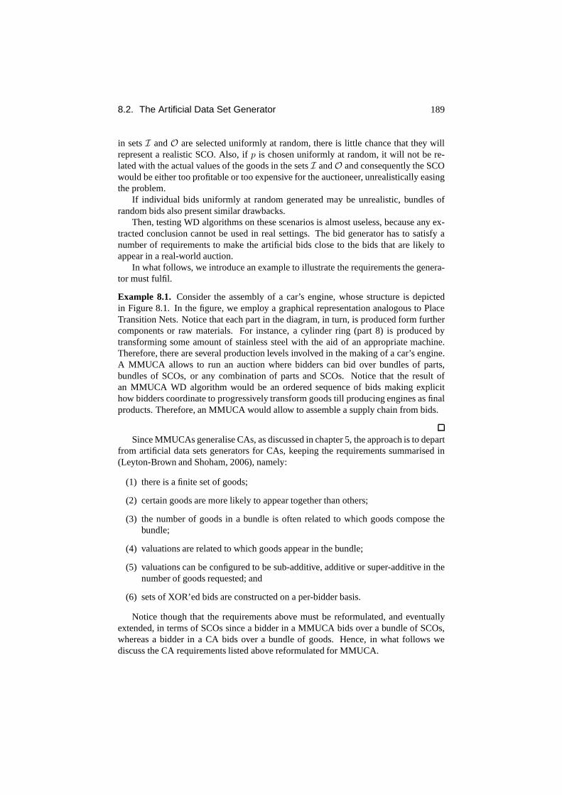
8.2. The Artificial Data Set Generator 189
in setsI andO are selected uniformly at random, there is little chance that they willrepresent a realistic SCO. Also, ifp is chosen uniformly at random, it will not be re-lated with the actual values of the goods in the setsI andO and consequently the SCOwould be either too profitable or too expensive for the auctioneer, unrealistically easingthe problem.
If individual bids uniformly at random generated may be unrealistic, bundles ofrandom bids also present similar drawbacks.
Then, testing WD algorithms on these scenarios is almost useless, because any ex-tracted conclusion cannot be used in real settings. The bid generator has to satisfy anumber of requirements to make the artificial bids close to the bids that are likely toappear in a real-world auction.
In what follows, we introduce an example to illustrate the requirements the genera-tor must fulfil.
Example 8.1. Consider the assembly of a car’s engine, whose structure is depictedin Figure 8.1. In the figure, we employ a graphical representation analogous to PlaceTransition Nets. Notice that each part in the diagram, in turn, is produced form furthercomponents or raw materials. For instance, a cylinder ring (part 8) is produced bytransforming some amount of stainless steel with the aid of an appropriate machine.Therefore, there are several production levels involved inthe making of a car’s engine.A MMUCA allows to run an auction where bidders can bid over bundles of parts,bundles of SCOs, or any combination of parts and SCOs. Noticethat the result ofan MMUCA WD algorithm would be an ordered sequence of bids making explicithow bidders coordinate to progressively transform goods till producing engines as finalproducts. Therefore, an MMUCA would allow to assemble a supply chain from bids.
Since MMUCAs generalise CAs, as discussed in chapter 5, the approach is to departfrom artificial data sets generators for CAs, keeping the requirements summarised in(Leyton-Brown and Shoham, 2006), namely:
(1) there is a finite set of goods;
(2) certain goods are more likely to appear together than others;
(3) the number of goods in a bundle is often related to which goods compose thebundle;
(4) valuations are related to which goods appear in the bundle;
(5) valuations can be configured to be sub-additive, additive or super-additive in thenumber of goods requested; and
(6) sets of XOR’ed bids are constructed on a per-bidder basis.
Notice though that the requirements above must be reformulated, and eventuallyextended, in terms of SCOs since a bidder in a MMUCA bids over abundle of SCOs,whereas a bidder in a CA bids over a bundle of goods. Hence, in what follows wediscuss the CA requirements listed above reformulated for MMUCA.

190 Chapter 8. Empirical Evaluation
Figure 8.1: Components of a car engine.
1. There is a finite set of SCOs.A CA generator bundles goods from a given set ofgoods to construct bids. What is the set of SCOs from which a MMUCA generatorconstructs bids? In order to provide a proper answer we must take inspiration on real-istic scenarios faced by buyers and providers. If so, withina given market we expectseveral producers to offer the very same or similar services(SCOs) at different prices,as well as several consumers to require the very same or similar services (SCOs) valuedat different prices. In other words, within a given market wecan identify a collectionof common services that companies request and offer. For instance, in the example inFigure 8.1, several providers may offer to assemble a cylinder through the very sameSCO:
t = (6′screws+ 1′cylinder line + 1′cylinder rig + 1′cylinder head, 1′cylinder)
Eventually, a provider may either offer to perform such SCO several times (e.g. asmany times as cylinders are required), or to bundle it with other SCOs, or the two.Hereafter, we shall consider the common goods and services in a given market to berepresented as a collection of SCOs that we shall refer to asmarket SCOs. Therefore,market SCOsare equivalent to thegoodsin a combinatorial auction, that is the objectproviders and buyers can request and offer. Hence, bids for MMUCAs shall becomposed as combinations of market SCOs. In this generator,the set of market SCOsis always finite and includes at least two market SCOs for every good inG, ensuringthat every good is individually available to buy and/or sell. As an example, Figure 8.2depicts a sample of market SCOs if intending to build the car engine in Figure 8.1.
8.2. The Artificial Data Set Generator 191
Figure 8.2: Market SCOs for a car’s engine.
2. Certain SCOs are more likely to appear together than others. In any market,services and goods are related to each other. For example, the production process fora good can also generate some by-products that can be sold with it or used in anotherindustrial process. Also, some services or products are usually bought together by thefinal customer.
3. There could be multiple copies of similar SCOs in a bundle.Since bids arecomposed as combinations of market SCOs, we must introduce the notion ofSCO mul-tiplicity as the counterpart of good multiplicity (the number of unitsof a given goodwithin an offer or a request). Say that in a CA a bidder submitsa bid for the goods inmulti-set{2′engine + 1′piston}. It is clear that the multiplicity of goodenginein thisbundle is two, whereas the multiplicity of goodpistonis one.
When SCOs are considered things change slightly. In fact, there are two ways toassign a multiplicity to SCOs, one is repeating the SCO several times , and the otherone is to simultaneously increase the required input goods and produced output goodswhile maintaining the same input/output ratio. For instance, consider the followingsupply chain operation
t = (3′a, 2′b) = (It,Ot) (8.1)
Then, we could repeat three times it either offering three times operationt, namely:
D = 3′t = 3′(3′a, 3′b) (8.2)
or triplicating both the input and output goods:
D = (3 · It, 3 · Ot) = (9′a, 6′b) (8.3)
192 Chapter 8. Empirical Evaluation
Notice that the semantics of the two types of multiplicity are different. On the onehand, equation (8.2) means that three copies of the same SCOsare offered and can beseparatelyused at three different steps of the solution sequence. On the other hand,equation (8.3) implies that the three copies must be employed at the very same step.That is, while in the former case there can be three differentsteps in the solution se-quence in which 3 copies of “a” are available, in the latter case the bidder needsninecopies if “a” available at a given step to perform the operation. Then, we will refer tothe multiplicity intended as in equation (8.3) asrepetition multiplicity, whereas to theone in equation (8.2) ascomponent-wise multiplicity.
4. Valuations are related to which SCOs appear in the bundle;furthermore SCOvaluations keep consistency with respect to bidder valuations for goods involvedin each SCO.A further issue has to do with the way bidders value SCOs and bundlesof SCOs. Notice that performing a SCO to assemble the engine in Figure 8.1 resultsin a new product that has more market value than its parts. Therefore, a car makervalues the SCO according to his expected benefits, namely thedifference between theexpected market value of the engine and the cost of its parts.Therefore, if the parts cost$850 and the expected market value of the engine is$1000, the car maker should bewilling to offer to pay less than$150 for the SCO. On the other hand, any provider isexpected to request less than$150 in order to perform the SCO. In general, buyers andproviders in a MMUCA should value a SCO on the basis of the difference between theexpected market value of its output goods and the cost of its input goods. Notice thoughthat we are not assuming here that such difference must always be positive. Likewisebidders should value bundles of SCOs considering the valuesof SCOs included in it.
5. Appropriate valuations can be configured to be sub-additive, additive orsuper-additive in the number of SCOs requested.This requirement tries to capturethe multiplicity-based (volume- based) discounts policies that are applied in real world.Significant discounts are applied in real markets when goodsand services are tradedat certain number of units. For example in figure 8.1, we observe that screws areusually traded in higher quantities than full engines. Thus, not surprisingly the same(percentage) discount may apply to an offer for 100 screws than to an offer for 5engines. Hence, an offer to produce more than 5 engines, being more unlikely, shouldreflect higher discounts.
6. Sets of XOR’ed bids are constructed on per-bidder basis.We recall from chapter5 that when a bidder submits different bids in XOR he declaresthat they are mutuallyexclusive offers. For example, the following offer
BID1(1′(1′engine, ∅), 100) XOR (8.4)
BID2(1′(2′engine, ∅), 190) (8.5)
stands for a bidder that offers to buy two engines or one engine but in any case threeengines. On the other hand when a bidder expresses complementarity he translates theOR bids as XOR bids. For example if a bidder wants to buy one engine or one cylinder

8.2. The Artificial Data Set Generator 193
he submits the following XOR-bid:
BID1(1′(1′engine, ∅), 100) XOR (8.6)
BID2(1′(1′cylinder, ∅), 30) XOR (8.7)
BID3(1′(1′cylinder + 1′engine, ∅), 120) (8.8)
As you can observe in both cases bids submitted in the same XORbid are likely to havesimilarities and, consequently, combining bids into XOR bids uniformly at randomdoes not capture this property.
7. Unrequested goods by the auctioneer may become involved in the auction.Finally, we add a last requirement that stems from the fact that, unlike auctioneers inCAs, not all goods involved in a MMUCA must be requested by theauctioneer. Backto our example of a car maker in need of engines depicted in Figure 8.1, it can run aMMUCA only requesting engines. Thereafter, bidders may offer already-assembledengines, or other goods (e.g. parts like crankcases, crankshafts, or screws) that jointlywith SCOs over such goods help produce the requested goods.
Figure 8.3: Modules of the bid generator and their interaction.
8.2.2 An Algorithm for Artificial Data Set Generation
In what follows we describe a bid generation algorithm that automates the generationof artificial data sets for MMUCA while capturing the requirements above. Thealgorithm’s purpose is to generate MMUCA WDP (each one composed of a collectionof XOR bids and the set of goods available to and requested by the auctioneer) thatcan be subsequently fed into an MMUCA WD algorithm. The algorithm starts bygenerating the set of goods involved in MMUCA. Next, it generates the goods theauctioneer requests. After that, it creates a subset of atomic SCOs, which are the

194 Chapter 8. Empirical Evaluation
market SCOs to employ for bid generation. Thereafter, it generates bids as linearcombinations of market SCOs, which are subsequently pricedaccording to a pricingpolicy. The resulting bids are further composed into XOR (mutually exclusive) bidsbecause the XOR language is fully expressive (as proved in section 5.3.6). Hence,the bid generation algorithm2 assumes that each bidder formulates a single XOR bid,being the number of bidders equal to the number of XOR bids. Infigure 8.3 we depictthe different modules of the generator and their interaction (Vinyals, 2007a).
Good Generation. This process requires the number of different goods (ngoods) in-volved in an auction along with the maximum price any good cantake on (maxPrice).Based on these values, it assesses for each goodg: (1) its average market price (µg)drawn from a uniform distributionU [1, maxPrice] wheremaxPrice stands for themaximum market price any good can take on; and (2) the distribution to assess itsmultiplicity, or more precisely, the success probability (ggeometric) of a geometricprobability distribution from which the good multiplicitycan be drawn.
Requested Goods Generation.This process assesses the number of units of eachgood the auctioneer requests, namely the multisetUout. Since the auctioneer must notrequest all goods, this process selects a subset of the goodsin G to be part ofUout.Firstly, it determines whether a goodg is requested by the auctioneer by comparing thevalue drawn from a uniform distributionU [0, 1] with pgood requested, the probability ofadding a new good toUout. Once a given goodg is included inUout, the number ofunits requested forg is drawn from a geometric distribution with the success probabilityggeometric obtained by the good generation process. Notice that by selecting a subsetof the goods we fulfil the requirement 7 listed in section 8.2.1 unrequested goods bythe auctioneer may be involved in the auction.
Market SCOs Generation. This process generatesa finite set of SCOsto be em-ployed as the building blocks to subsequently compose bids and consequently fulfillingrequirement 1 listed in section 8.2.1. For each good, this procedure constructs two mar-ket SCOs, one with only input goods (I-SCO) and one with only output goods (O-SCO).Each SCO involves a single good with multiplicity one. For instance,({engine}, {})and({}, {engine}) stand respectively for the I- SCO and O-SCO for goodengine. Af-ter that, the algorithm generates a limited number of marketSCO (IO-SCOs) with bothinput and output goods (nIO market SCOs). In order to generate each market IO-SCO,this procedure chooses the goods to include in its input and output set employing theprobabilities of adding some good to the input and output setrespectively (pgood in input
andpgood in output). Whenever a good is included to either the input or output set, itsmultiplicity is calculated from a geometric distribution parametrised byggeometric.
Finally, we attach to each market SCO a probability distribution to draw itscomponent-wise multiplicity. It is assumed that the bid generation process, detailedby algorithm 1, uses a geometric distribution to calculate the component-wise multi-plicity of each market SCO. Hence, the generation of market SCOs assesses the success
2Here we only provide the bid generation algorithm. The interested reader must refer to (Vinyals, 2007b)for a complete description of all algorithms required by theartificial data set generator.

8.2. The Artificial Data Set Generator 195
probability to be employed by such geometric distributions, namely the probability ofadding an extra unit of a SCO already included in a bundle bid.Thus, each SCOtis assigned a success probabilitytgeometric. However, success probabilities cannot beuniformly at random generated because SCOs are defined over multisets of goods, andtherefore consistency must be kept with respect to the success probabilities assigned toeach good by the good generation process. Therefore, the success probability for eachSCO is set as follows. Given a SCOt = (I,O), for each goodg involved in the SCO,The success probability oft is set to:
tgeometric = ming∈G
g|mI(g)−mO(g)|geometric (8.9)
wheremI(g) (respectivelymO(g)) stands for the number of occurrences ofg in I(respectivelyO).Bid Generation. The bid generation algorithm (algorithm 1) generates bids that aresubsequently combined into XOR bids, each one encoding the offer or request of abidder. This process makes explicit:
(1) which SCOs and how many of them to offer/request in a bundle;
(2) how to price the bundle; and
(3) which bids to combine in an XOR bid.
In what follows we detail each of this functions:
(1) Selecting the SCOs requested in a bundle and their multiplicities. Firstly, foreach XOR bid (XORBid ) the algorithm composes each bid (Bid ) by combiningthe market SCOs (MTS ) returned by the market SCO generation process. Thenumber of market SCOs (nTransfBid ) to compose each bid is obtained from anormal distributionN (µadd new SCO, σadd new SCO) (line 12).
Market SCOs are chosen from the set of market SCOs (MTS ) and theircomponent-wise multiplicityin the bundle bid is obtained from a geometric
distribution with success probabilitytgeometric (line 15-16). By assessing thenumber of units to include in a bundle using a probabilistic distribution that de-pends on each SCO we partially fulfil requirement 3:there could be multiplecopies of similar SCOs in a bundle. In fact, in this way SCOs repeated as inequation (8.3) are likely to appear. In this way the authors provide arepetitionmultiplicity associated to SCOs as well.
We also consider that, given an existing bundle, not all SCOsare equally likelyto be requested becausecertain SCOs (for which complementarities hold) will bemore likely to appear together than others, as stated by requirement 2 in section8.2.1. To ease these complementarities we assume that the probability of addinga new market SCO to an existing bundle only depends on the lastSCO added andnot on the whole bundle (Markov property).
It is clear that different copies of the same SCOs may be included in the solution.That is, we may haverepetitionsof SCOs (as the one in equation (8.2)). Then,requirement 3 is completely fulfilled.

196 Chapter 8. Empirical Evaluation
(2) Pricing the bundle. Next, the algorithm prices the SCO according to itscomponent-wise multiplicity(lines 17-21). To fulfil valuations requirementslisted in section 8.2.1, a pricing policy must provide the means to price a good,
Algorithm 1 Bid Generation(MTS, nXOR bids, µ, σprices, µadd new XOR clause,σadd new SCO, µadd new SCO, σadd new SCO, α)
1: for g = 1 to ngoods do2: for b = 1 to nXOR bids do3: pprices bid[b, g]← µ[g] ·N(1, σprices)4: end for5: end for6: Bids← ∅7: for b = 1 to nXOR bids do8: XORBid← EmptyXORBid()9: nXORClauses← N (µadd new XOR clause, σadd new XOR clause)
10: for x = 1 to nXORClauses do11: Bid← EmptyCombinatorialBid()12: nTransfBid← N (µadd new SCO, σadd new SCO)13: if x == 1 then14: for t = 1 to nTransfBid do15: MT ← Select a SCO using Markov model fromMTS with stateMT16: multiplicity ← Geometric(MT.tgeometric) bid B.17: T.inputs←MT.inputs ·multiplicity18: T.outputs←MT.outputs ·multiplicity19: T.price←
P
g∈T.outputs
pprices bid[b, g]−P
g∈T.inputs
pprices bid[b, g]
20: poffer ← (T.tgeometric)multiplicity
21: discount← α 1−e1−poffer
1−e
22: Bid.t← Bid.t ∪ T23: Bid.price← Bid.price + T.price · (1− discount)24: end for25: else26: model←Uniformly At Random generate a number between 1 and x-127: Bid← XORBid(model)28: if nTransfBid ≥ length(XORBid(model).t) then29: Bid← removeRandomTransition(Bid)30: Bid← recalculatePrices(Bid)31: end if32: if nTransfBid ≤ length(XORBid(model).t) then33: Bid← addRandomTransition(Bid)34: Bid← recalculatePrices(Bid)35: end if36: end if37: XORBid← XORBid ∪ {Bid}38: end for39: Bids← Bids ∪ {XORBid}40: end for41: return Bids

8.2. The Artificial Data Set Generator 197
a SCO, multiple units of the very same SCO, and a bundle of SCOsin a realisticmanner. As to pricing goods, in order to vary prices among bidders, the algorithmgenerates a price for bidderb for goodg, represented aspprices bid[b, g], froma normal distributionN (µ[g], σprices), whereµ[g] stands for goodg’s averageprice in the market andσprices for the variance among bidders’ prices (lines 2-4).Thereafter, a SCO’s price for bidderb is assessed in terms of the difference fromhis valuation of its output goods with respect to his valuation of its input goods(line 19). Accordingly,SCO valuations keep consistency with respect to biddervaluations for goods involved in each SCOas stated by requirement 5 in section8.2.1. Each bid valuation is obtained by adding the prices ofits SCOs (line 23).Hencevaluations are related to which SCOs compose the bundleas stated by re-quirement 6 although varying among different bidders. Furthermore we proposeto introduce super-additivity by applying multiplicity-based discounts to SCOsaddressing the requirement thatvaluations can be configured to be sub-additive,additive o super-additive in the number of SCOs requested. In other words, asa general rule, the more unlikely for a SCO to be traded at certain units (multi-plicity), the higher the discount to apply to its overall price. In this way we tryto capture in a realistic manner the way multiplicity-based(volume-based) dis-counts are applied in the real world. Therefore, given SCOt, we firstly assessthe probabilitypoffer of the SCO to be traded withcomponent-wise multiplicitym from a geometric distribution with success probabilitytgeometric as follows:poffer = tgeometric
multiplicity (line 20). Secondly, we compute the discount
to apply (discount) as follows:discount = α 1−e1−poffer
1−e. Indeed, in this way
we manage to apply higher discounts to more unlikely offers within the range[0, α]. Notice too that settingα to zero leads to no discounts, and thus to nosuper-additivity.
(3) Which bids to combine in an XOR bid.Finally, after creating each bid, thealgorithm adds it to the XOR bid under construction (line 37). The num-ber of bids that compose an XOR bid is obtained from a normal distributionN (µadd new XOR clause, σadd new XOR clause) (line 9). We consider here require-ment 7 listed in section 8.2.1 and since different bids in XOR-relationships standfor different alternatives or options for the bidder we propose to generate similarbids for the same XORBid. The first bid of each XORBid is generated uniformlyat random (lines 13-24) whereas the rest of bids are created applying some mod-ifications over one existing bid in the bundle (lines 25-36).The number of modi-fications depends on the difference between the number of SCOs assigned to thenew bid and the existent one:
• if it is less we remove randomly one SCO;
• if it is greater we add uniformly at random new SCOs; and
• if it is equal we apply once both operations.
In all cases we finally recalculate the prices following the proposed price policy.Hence the requirement thatsets of XOR’ed bids are constructed on a per-bidderbasisis fulfilled.

198 Chapter 8. Empirical Evaluation
ngoods 20nIO market SCOs n SCOs/3
max price 100σprices 0.05pgood requested 0.3µadd new SCO 1.0σadd new SCO 0µadd new XOR clause 1.0σadd new XOR clause 0pgood in input 0.2pgood in output 0.1α 0.1p ISCOs 0.6p OSCOs 0.1allow cycles 1
Table 8.1: Artificial generator parameter values.
8.3 Empirical Evaluation
In this section, we firstly provide a preliminary comparisonof DIP and CCIP on ar-bitrary supply chain network topologies. Next, we run the CMWOSP-based solver onacyclic network topologies.
8.3.1 DIP versus CCIP
In what follows, we provide a preliminary experiment to quantitatively assess the sizeof the supply chain formation scenarios that CCIP allows to solve compared to DIP.
According to (Hillier and Lieberman, 1986), the number of decision variables is agood index of the difficulty of an optimisation problem (although not the only one).Since the number of decision variables of both DIP and CCIP depend on the number ofSCOs within the submitted bids, in order to compare their computational performancesand to analyse their scalability, we have chosen to observe their solving times as thenumber of SCOs increases. In order to compare the DIP and CCIPMMUCA WDalgorithms, we have employed randomly generated MMUCA WDPsusing the artificialdata set generator presented in section 8.2. We have set the generator parameters forthis experiment as listed in Table 8.1.
We ran our experiments as follows. We generated MMUCA WDP instances withSCOs within the range[0, 300]. We sampled the interval to generate 50 WDP instancesevery 20 SCOs. Both solvers DIP and CCIP were fed with the verysame WDP in-stances. We solved each WDP instance using implementationsof both solvers onCPLEX 10.1 (ILOG, 2007), recording both the solutions and solving times. More-over, we set a maximum time limit to 4800 seconds for each solver to find a solution foreach WDP instance. Whenever any of the solvers exceeded the time limit, we markedthe WDP astime exceededand assigned. After that, we set its solving time to the time

8.3. Empirical Evaluation 199
Figure 8.4: Comparison between DIP and CCIP.
limit to subsequently record it. Notice that we only considered feasible WDP instancesto calculate solving times since the time required by CPLEX to prove unfeasibility is(usually) significantly lower than the time required to find an optimal solution. Finally,we ran all tests on a Dell Precision 490 with double processorDual-Core Xeon 5060running at 3.2 GHz with 2Gb RAM on a Linux 2.6.
Figures 8.4 and 8.5 summarise the results of this experiment. Figure 8.4 depicts themedian of the solving times obtained when varying the numberof SCOs. Figure 8.5shows for both DIP and CCIP the number of instances that have been solved withinthe time limit. Then, given a time limit, CCIP was able to solve problems with morethan twice the number of SCOs than DIP did solve. Indeed, whereas 120 representsthe empirical limit (∼50% of solved instances) on the number of SCOs for DIP, CCIPstarts reaching the time limit when solving WDP instances containing more than 250SCOs. Furthermore, for WDPs with close to 100 SCOs, DIP is in median about 70times slower than CCIP. This ratio rapidly increases as the number of SCOs gets closeto 120 in the presented scenario.
The observations stemming from this experiment are very promising. They in-dicatethat we can obtain substantial reductions in the solving time when employingCCIP instead of DIPdepending on the features of the scenario. The search space reduc-tion obtained with solver CCIP translates into a significantdecrease in computationalsolving time complexity.

200 Chapter 8. Empirical Evaluation
Figure 8.5: Number of instances solved within the time limit(4800 sec.).
8.3.2 Performances of the CMWOSP-based solver
In this section we aim at testing the performances of the CMWOSP algorithm (that canbe used only when theMixed Auction Netis acyclic). Recall that (section 7.3.3) at thetheoretical level the CMWOSP-based and CCIP solvers are equivalent when theMixedAuction Netis acyclic. However, if we employ CCIP we should compute the stronglyconnected components beforehand. In this case, since we a-priori know that theMixedAuction Netis acyclic, we directly employ the CMWOSP-based solver.
We have run this experiment as described in section 8.3.1, but enforcing the bidgenerator to build instances with no cycles. Figure 8.6 shows the CPU time required tosolve problem instances on acyclic nets for the CMWOSP-based solver.
Notice that the axis time scale in figure 8.6 is nearly four orders of magnitudesmaller than in figure 8.4. Hence, cycles in the mixed auctionnet may lead to a signifi-cant increase in computational cost.
8.4 Conclusions
In this chapter we presented a preliminary empirical comparison of the CMWOSP-based, DIP and CCIP solvers. Firstly, we compared DIP and CCIP on any type of

8.4. Conclusions 201
40 60 80 100 120 140 160 180 200 220 240 260 280 3000
0.05
0.1
0.15
0.2
0.25
0.3
0.35
Number of SCOs
Med
ian
Sol
ving
Tim
es (
sec.
)
CMWOSP solver
Figure 8.6: Experiments with acyclic network topologies (reduced time scale).
network topology. Next, we empirically assessed the performances of the CMWOSP-based solver on acyclicMixed Auction Nets.
In chapter 7, we proposed CCIP, a solver that dramatically improves the computa-tional efficiency of DIP by taking advantage of the topological characteristics of WDPs.At the theoretical level, we proved that CCIP brings a drastic reduction in the numberof decision variables required to solve the WDP. In this chapter, we have empiricallyobserved that in the presented scenario CCIP:
(1) can deal with WDPs with more than twice SCOs than DIP;
(2) can significantly reduce the computation time (by a factor larger than 70).
Finally, we observed that in the considered parameter setting the CMWOSP-basedsolver is four orders of magnitude faster in solving acyclicinstances than DIP andCCIP in solving instances produced by Vinyals’ generator.


Chapter 9
Conclusions and Future Work
In this chapter, we draw some conclusions about the work developed in this dissertationand we show some open paths to future development.
9.1 Conclusions
Most of the currently studied and employed combinatorial auctions deal with the nego-tiation of goods, disregarding eventual production relationships holding among them.The information about such relationships helps improve theoutcome of a negotiation.In order to fill this gap, we introduced two novel combinatorial auction extensions thathelp in determining the revenue-maximising strategy for partner selection in supplychain network design and planning. The former, calledMulti Unit Combinatorial Re-verse Auctions with Transformability Relationships amongGoods (MUCRAtR), copeswith make-or-buydecisions. The latter, calledMixed Multi-unit Combinatorial Auc-tions (MMUCA), deals withmake-or-buy-or-collaboratedecisions. Below, we sepa-rately summarise our two contributions.
9.1.1 Make-or-Buy Decisions
In chapter 1, we thoroughly described the requirements thatmust be fulfilled in order tosolvemake-or-buydecision problems. Since we built upon combinatorial auctions, wealso explained the of CAs limitations that hinder their application to our problem. Intable 9.1 we recall both the requirements and the corresponding CAs limitations associ-ated with themake-or-buydecision problem. We observed that all the CAs limitationsstem from the fact that they can neither express nor represent an auctioneer’s internalmanufacturing operations.
The first requirement hindering the application of CAs to ourproblem is that theycan neither represent internal manufacturing operations nor the producer/consumer re-lationships among them. In order to apply CAs to solve themake-or-buydecision prob-lem, we provided a formal framework to represent internal manufacturing operations.At this aim we decided to employ Place/Transition Nets (PTNs) (Reisig, 1985) because:
203

204 Chapter 9. Conclusions and Future Work
Requirements CAs MUCRAtR1 express a request on bundles of goods X X
2 express an auctioneer’s initial stock X
3 express producer/consumer relationships among internal operations X
4 specify an auctioneer’s final requirements X
5 express relationships among manufacturing operations,auctioned goods, and received bids X
6 formally and graphical represent the search spaceassociated to the auctioneer’s decision problem X
7 specify the auctioneer’s internal cost structure X
8 information about which in-house operations to performand in which order X
Table 9.1: Requirements of to themake-or-buyproblem.
(1) they naturally help us capture the notion of manufacturing operation;
(2) they have a well-defined semantics that can naturally accommodate the notion ofsequence of operations and consumer/producer relationships;
(3) they have an integrated description of both states and actions to characterise thesearch space where operations occur;
(4) they have a large number of formal analysis methods that allow the investigationof structural and behavioural (dynamic) properties of the net; and
(5) they have a graphical representation that is intuitively very appealing to studyproblems related to the topology of the supply chain.
Thus, we modelled the internal production structure of an auctioneer by means of aPTN, that we referred to asPTNI . Not only does this formal representation allow usto describe the quantity of resources either produced or consumed by a manufacturingoperation, the producer/consumer relationships among operations, and the quantity ofgoods available to an auctioneer after each operation, but it also allow us to expresspreconditions over a manufacturing operation by means of afiring rule. By the appli-cation of the firing rule, we impose that a manufacturing operation canonly be run ifits input goods are available. This property is critical forthe correct representation of aproduction process: the implementation order of a production process is constrained bythe availability of resources at each step.
Then, aPTNI completely specifies an auctioneer’s internal manufacturing oper-ations and the producer/consumer relationships among them(requirement (5) in table9.1). Moreover, aPTNI allows an auctioneer to specify his requirements and com-municate them to bidders (requirement (4) in table 9.1). This is obtained by specifyinga configuration (marking) to end up with. If an auctioneer communicates to a set ofbidders hisPTNI along with a description of the final state of such PTN describinghis requirements, then the bidders can infer all the possible configurations of offersfulfilling such requirements.

9.1. Conclusions 205
Next, in order to express the relationships among internal manufacturing operations,auctioned goods, and received bids ( requirement (3) in table 9.1), we incorporated thereceived bids intoPTNI . At this aim, we exploited the fact that a bid that offers goodscan be regarded as a transition (bid transition) that injects tokens intoPTNI . Unliketransitions corresponding to manufacturing operations, bid transitions do not consumeinput resources and can be fired only once. ThePTNI augmented with bid transitionswas calledPTNE (whereE stands forExtended).
By means of aPTNE, an auctioneer can compactly express all the possible out-comes of any of his possible decisions. By decision we mean the selection of bidstogether with a sequence of internal operations to perform.Thus, aPTNE both for-mally and graphically represents the search space associated to the auctioneer’s deci-sion problem (requirement 6 in table 9.1). We successfully linked bids, manufacturingoperations, and goods at auction, and we fully represent allthe possible decisions anauctioneer may take in a unified representation.
However, the goal of the auctioneer is not only to find a feasible outcome, but alsoto find an outcome that minimises his costs. Thus, an auctioneer needs to quantify thecost associated to each decision. With this aim, he has to associate a cost to the selectionof a bid, and a cost to the performance of a manufacturing operation. Unfortunately,in their original definition, place transition nets do not incorporate the notion of costassociated to the firing of a transition. Then, we defined a newtype of Place TransitionNet, the so-calledWeighted Place Transition Nets(WPTN), to express the notion ofcost associated to transition firings or to the firing of sequences of transitions.
Then, we transformed bothPTNI andPTNE into WPTNs by associating to eachoperation transitionthe cost of the corresponding manufacturing operation and to eachbid transitionthe bid cost. The resulting WPTNs were calledTransformability NetworkStructure(TNS) andAuction Netrespectively: a TNS completely describes an auction-eer’s internal manufacturing operations, whereas an Auction Net compactly representsthe set of possible auctioneer’s decisions along with the corresponding cost. Then,Transformability Network StructureandAuction Netallow the auctioneer to express hisinternal cost structure and to incorporate it into his decision problem (requirement (7)in table 9.1).
The auctioneer needs to select the set of offers along with the sequence of internalmanufacturing operations to perform that minimise his costs and allow him to obtainhis final requirements (point (8) in table 9.1). With this purpose, we defined the auc-tioneer’s decision problem as an optimisation problem on the Auction Net. Thus, weintroduced a new type of reachability problem over WPTNs, and called this new op-timisation problem theConstrained Maximum Weight Occurrence Sequence Problem(CMWOSP). Intuitively, this optimisation problem involves finding an optimal costsequence of transitions on a WPTN that leads to a final state which fulfils some con-straints.
Additionally, we provided an important result on the CMWOSP. We showed thatthe CMWOSP can be solved by means of Integer Programming on acyclic WPTNs,namely on WPTNs that do not contain any directed cycle.
The CMWOSP perfectly captures the semantics of the auctioneer’s decision prob-lem in a MUCRAtR: to find the set ofbid and operation transitionsthat minimises

206 Chapter 9. Conclusions and Future Work
an auctioneer’s revenue. Thus, we formalised the auctioneer’s decision problem in aMUCRAtR as a CMWOSP on the Auction Net. Two major benefits, andthereforecontributions, stemmed from the formalisation of the MUCRAtR WDP by means of aCMWOSP:
(1) the CMWOSP provides as a result both the set of bids to accept and the sequenceof operations to perform in order to obtain the auctioneer’sfinal requirements(requirement (8) in table 9.1);
(2) themake-or-buydecision problem can be solved by means of Integer Program-ming for a large class of supply chain network topologies (acyclic).
Summarising, we provide to the auctioneer with a formalism to express his require-ments and communicating them to bidders; and a rule for determining the optimal allo-cation, i.e. the set of winning bids and the sequence of internal operations to perform.In this way we provide a solution to all the requirements needed for extending combi-natorial auctions for dealing with themake-or-buydecision problem.
The solution to the WDP that we provide can be employed as a decision supportsystem in different settings:
• Combinatorial auctions. As a winner determination solver in a MUCRAtR.
• Negotiation. A buyer, after receiving a set of offers from his providers,can com-pute the best offers and eventually counter-offer.
• What-if supply chain analysis. A buyer, aware of the prices and capacities of hisproviders, can test different configurations of his supply chain.
Summary of MUCRAtR contributions
To summarise, the main contributions related to themake-or-buydecision problem are:
• MUCRAtR , an extension of combinatorial auctions that allows dealing withmake-or-buydecision problems in scenarios characterised by combinatorial pref-erences. This new auction type provides an auctioneer with aframework to opti-mise his outsourcing strategy.
• Weighted Place Transition Nets (WPTN), an extension of Place TransitionNets. In WPTNs it is possible to associate a weight (cost) to the firing of eachtransition. WPTN is a formal framework introduced to represent the MUCRAtRspace of auctioneer’s decisions and associated revenues.
• Constrained Maximum Weighted Occurrence Sequence Problem(CM-WOSP), a new reachability problem defined on WPTNs. It formalises the prob-lem of selecting a cost-maximising sequence of actions leading from an initialstate to a set of possible final states.
• ILP solution to the CMWOSP. We prove that the CMWOSP can be solved bymeans of ILP when the underlying WPTN is acyclic. We obtain this contributionby exploiting results imported from the literature on PlaceTransition Nets.

9.1. Conclusions 207
• Formalisation of the MUCRAtR WDP as a CMWOSP on an Auction Net.We show that CMWOSP perfectly captures the features of the auctioneer’s de-cision problem in a MUCRAtR. This results provides three important benefits:(1) an ILP formulation for a wide class of MUCRAtR WDPs (acyclic); (2) a for-malism (PTN) to analyse the decision problem; and (3) the result of the WDPprovides both the set of selected bids and thesequenceof operations to perform.
9.1.2 Make-Or-Buy-Or-Collaborate
In the second part of this dissertation we dealt with themake-or-buy-or-collaboratedecision problem. As thoroughly explained in section 1.4.2, most of the requirementsarising in themake-or-buy-or-collaboratedecision problem are currently not supportedby state-of-the-art methodologies and tools. In table 9.2 we summarise the requirementsand the limitations of two state-of-the-art solutions, namely combinatorial auctions andtask dependency networks.
MMUCA
In order to overcome such limitations, we introduced an extension to combinatorialauctions, calledMixed Multi-unit Combinatorial Auctions(MMUCA), that fulfils allthe requirements of this decision problem.
Requirements CAs TDN1 express an offer/request on bundles of goods X X
2 express an offer of a SCO with a single output product X
3 express an offer of a SCO with multiple output products4 express a request of a SCO5 express the offer/request of a bundle of SCOs6 express combinations of bids X
7 express the min/max number of times SCOs are performed8 express resource sharing9 express an auctioneer’s initial stock10 express the auctioneer’s final requirements11 supportacyclicsupply chain networks X
12 supportcyclic supply chain networks13 compute thescheduled sequenceof SCOs to perform14 ensure computational tractability while preserving optimality15 solve SCF decision problem X
16 solve themake-or-buy-or-collaboratedecision problem17 formally represent the search space18 graphically represent the search space19 assess the computational tractability based on the problemstructure
Table 9.2: Requirements of themake-or-buy-or-collaborateproblem.
MMUCAs support the trading of operations across the supply chain: from the sup-ply and demand of components to the supply and demand of manufacturing operations
208 Chapter 9. Conclusions and Future Work
or services. With the aim of making MMUCA operative:
(1) we provided a formal language allowing bidders to express offers and requestsover supply chain operations; and
(2) we formalised the optimisation problem faced by an auctioneer aiming at select-ing the subset of the offered supply chain operations maximising his revenue.
As to the formal language, we introduced a general-purpose concept that can rep-resent any operation or service negotiated across the supply chain by any supply chainstakeholder, the so-calledsupply chain operation(SCO). The characterising featuresof SCOs are the required and consumed input resources and theoutput resources pro-duced by the service. According to requirements (1-8) in table 9.2, the different actorsinvolved in a MMUCA require a language to express the offer/request of supply chainoperations. Then, we extended traditional bidding languages in the literature to dealwith SCOs.
Bidding Language
We set SCOs as the atomic entities that can be negotiated across a supply chain. Build-ing upon such building blocks, we defined a new bidding language that allows bidders:
(1) associating a value to bundles of SCOs within anatomic bid; and
(2) combiningatomic bidsinto complex expressions encoding a wide variety of pref-erences over SCOs.
The provided bidding language generalises state-of-the art bidding languages andprovides supports to express bids in the following auction types:
• Multi-unit combinatorial auctions, where there may be several indistinguishablecopies of the same good available in the system.
• Double auctionswhere there are multiple buyers and multiple sellers. We inte-grate direct and reverse auctions,i.e. the auctioneer will be able to both sell andbuy goods within a single auction. Or considering the bidders’ point of view, abidder can submit both offers and demands on sets of goods.
• Combinatorial exchanges. Combinatorial case of double auctions. In this auctiontype both buyers and seller submit combinatorial bids.
• Multi-unit Combinatorial Reverse Auctions with Transformability Relationshipsamong Goods(MUCRAtR). We integrate the notion of internal manufacturingoperation into MMUCAs.
• Combinatorial auctions for supply chain formationintroduced in(Walsh et al., 2000).

9.1. Conclusions 209
The novelty of our bidding language with respect to the above-mentioned auction typesis that we further extend the idea of manufacturing operations by allowing agents to alsobid for supply chain operations. Since in our language a bidder is allowed to bid overbundlesof supply chain operations, such language captures potential complementaritiesamong such operations. This extension offers a higher degree of expressiveness andallows to generalise bidding languages for the above-listed auction types.
Summarising, the proposed bidding language can express several types of complexbids and allows for bids on bundles of SCOs. By means of the introduced biddinglanguage we overcome requirements (1-8) in table 9.2.
The Winner Determination Problem
As to the Winner Determination Problem, we cannot rely on previous definitions in theliterature. According to requirement (13) in table 9.2, andsimilarly to MUCRAtR, anew dimension comes into play: theorder among SCOs. For this reason, we provideda new and general definition of winner determination problemthat builds upon ourSCO-based bidding language. The WDP describes the rules to:
• select the winning bids that maximise an auctioneer’s revenue; and
• assess theexecution orderof the SCOs contained in the winning bids.
Notice that the winning bids are those that:
• they fulfil the constraints specified by bidders via the bidding language;
• they maximise the auctioneer revenue.
and the sequence of SCOs representing the execution order issuch that:
• it contains all and only the SCOs included in the winning bids;
• it is implementable, i.e. each SCO in the sequence must have its required inputsavailable at the position where it is scheduled; and
• it produces at its end at least the set of goods required by theauctioneer.
Observe that theorder in which agents consume and produce goods is of central impor-tance in our model and affects the definition of the winner determination problem.
The rule to assess the set of winners provides a solution to requirements 10, 13,15, and 16 in table 9.2. By including the constraint that the goods available after run-ning all the selected supply chain operations are the ones specified by the auctioneer,we provided a solution to requirement (9) in table 9.2. Sincethe definition does notdepend on the particular topology of the supply chain network, we provided a solutionto requirement (11-12) in table 1.2.
The new WDP definition extends and generalises the definitionof winner determi-nation for:
• Multi-unit combinatorial auctions
210 Chapter 9. Conclusions and Future Work
• Double auctions
• Combinatorial exchanges
• MUCRAtR
• Combinatorial auctions for supply chain formation
Thus, we provided both a bidding language and a definition of winner determinationproblem that extends and generalises all the above-mentioned auction types. The bid-ding language along with the winning rule fully characterisesMixed Multi-unit Combi-natorial Auctions(MMUCAs).
A mathematical framework for the MMUCA WDP
Analogously to the MUCRAtR WDP, we provided a mapping of the MMUCA winnerdetermination problem to aConstrained Maximum Weight Occurrence Sequence Prob-lemon theMixed Auction Net. Via this mapping, we obtained the same advantages asin the case of MUCRAtR: (1) the solution is expressed as asequenceof SCOs; (2) weprovide a formal framework to analyse the properties of the decision problem; and (3)we obtain an ILP-based formulation of the MMUCA WDP for acyclic Mixed AuctionNets.
The Mixed Auction Netprovides a formalism to reason about MMUCAs,and therefore also about all the WDPs associated to auctionssubsumed byMMUCA (requirements (17-18) in table 9.2). In particular, we showed that theMixed Auction Netsubsumes the TNS and the Transformability Network Structure(Walsh and Wellman, 2003).
Solving the MMUCA WDP
In this dissertation we provided three different IP solversfor computing the solutionsto the MMUCA WDP. The first one is based on the mapping to CMWOSP. This solverdeals with acyclic supply chain network topologies. The second one (DIP) was directlybuilt upon the definition of MMUCA WDP and applies to arbitrary network topologies.The third one (CCIP) improves the performances of the secondsolver by exploitingsome domain knowledge.
The CMWOSP-based Solver. By mapping to CMWOSP we obtain an ILP-basedformulation of the MMUCA WDP with integer programming for a wide class of WPTNtopologies.
The DIP Solver. We showed that restricting the Mixed Auction Net to be acyclic isa significant limitation in some scenarios: it does not allowrepresenting cyclic oper-ations, resource sharing, and so on. We provided a new IP formulation, calledDirectInteger Programming(DIP) solver, that is directly built upon the definition of MMUCAWDP. DIP solves the WDP associated to any supply chain network topology, thusbroadening the classes of solvable problems.
9.1. Conclusions 211
The CCIP solver. The main drawback of DIP is that it generates a number of decisionvariables and constraints that limit its applicability to small-size and medium-size sce-narios. DIP guarantees optimality, but decrements the computational tractability. Weproposed an ILP-based formulation for MMUCA WDP, namely theConnected Compo-nent Based Integer ProgrammingSolver (CCIP), that dramatically improves the com-putational efficiency of DIP. A search space reduction is achieved by analysing andexploiting the precedence relationships among SCOs.
We conclude by observing that our approach solves some of theproblems relatedto centralised approaches to supply chain formation and scheduling (see section 3.3.1).Firstly, we can reduce the complexity associated to optimise the scheduling problem.In fact, we have that
• the complexity of the scheduling problem is reduced due to the absence of timedimension, without losing the possibility to express precedence relationshipsamong operations; and
• we provide a very efficient optimisation problem solver (CCIP).
Secondly, agents are not forced to reveal all their information truthfully. The part ofinformation revealed by agents (the bidders) is regulated by the bidding language andthe market-based mechanism. In market-based mechanisms agents can act strategically,hide or lie on critical information, decide what to communicate and what not.
Empirical Evaluation
In the last part of this dissertation we provided a preliminary proof of concept aboutthe performances of the CMWOSP-based, DIP and CCIP solvers in a single scenario.On the one hand, we compared DIP and CCIP on arbitrary networktopologies. On theother hand, we empirically assessed the performances of theCMWOSP-based solveron acyclicMixed Auction Nets. We observed that in the considered parameter setting:
• CCIP outperforms DIP
• acyclic instances are much easier to solve
Summary of MMUCA Contributions
To summarise, the contributions in this dissertation related to themake-or-buy-or-collaboratedecision problem are listed in what follows.
• MMUCA is a new type of auction that allows to deal withmake-or-buy-or-collaboratedecisions. This new auction type provides an auctioneer with aframework to optimally select supply chain partners. MMUCAgeneralises andextends several types of auctions (including MUCRAtR). Ourcontribution devel-ops along two dimensions:
– MMUCA Bidding Language. We provide a novel bidding language thatallows agents to trade any type of operation across the supply chain. Sucha language extends and generalises several previous bidding languages.

212 Chapter 9. Conclusions and Future Work
– MMUCA Winner Determination Problem . We provide a definition ofwinner determination problem that selects, among the received bids, therevenue-maximisingordered sequenceof supply chain operations to per-form. The definition of MMUCA WDP extends and generalises thedefini-tion of winner determination problem of several existing auction types.
• Mixed Auction Net is a WPTN that compactly represents the space of possibledecisions an auctioneer may take, along with the revenue associated to each de-cision. Thus, it formally and graphically represents the search space associatedto the MMUCA WDP, and therefore of themake-or-buy-or-collaboratedecisionproblem.
• Mapping the MMUCA WDP to the CMWOSP . We succeeded in mapping theMMUCA WDP to a CMWOSP on theMixed Auction Net. As in the case ofMUCRAtR, three benefits stemmed from this mapping: (1) the provided solutionis a sequence of SCOs; (2) a whole corpus of theoretical results from the PTNliterature can be imported to analyse the decision problem;and (3) we obtain anILP formulation of the WDP for acyclicMixed Auction Nets.
• MMUCA WDP Solvers.
– CMWOSP-Based Solver. This ILP-based solver is based on the mappingof MMUCA and MUCRAtR to a CMWOSP and applies only to acyclicmixed auction nets.
– DIP solver. This ILP-based solver works on arbitrary supply chain networktopologies. It overcomes a set of limitations connected with the use of theCMWOSP-based solver.
– CCIP solver. This ILP-based solver dramatically improves the perfor-mances of DIP solver because it allows a more concise representation ofthe optimisation problem. This is obtained by exploiting the precedencerelations among supply chain operations.
Finally, consider that MUCRAtR and Combinatorial Auctionsfor supply chainformation are a special case of MMUCA. Thus, the three solvers presented abovecan be used to solve problems on any network topologies for them as well. Thus,besides broadening the applicability of MMUCAs, we have also broadened theapplicability of MUCRAtR and CAs for SCF. MUCRAtR and CAs forSCF canbe extended to any network topology!
9.2 Future Work
We believe that this dissertation opens several paths to future developments. The mostinteresting extension we envisage to MMUCAs is the incorporation of time and uncer-tainty in the MMUCA model.
On the one hand, we envisage the possibility to express the release time and durationof a supply chain operation. This information should be alsoincluded within the winner
9.2. Future Work 213
determination problem. In this way, an auctioneer would be able to fix deadlines to havehis production process completed. Moreover, the participants to the supply chain wouldsynchronise their operations by fulfilling not only the producer/consumer relationships,but also eventual time constraints.
On the other hand, an auctioneer may be interested in assigning a success proba-bility to each supply chain operation. In this way, he could minimise the incidence offailures and shortcoming across the supply chain.
Next, in order to outperform CCIP we plan to explore the design of a local algo-rithm. Although solutions may be sub-optimal with a local approach, the number oftransformations that can be dealt with is expected to be larger, and hence the size of thesupply chain scenarios we could tackle.
Furthermore, a more realistic setting requires to incorporate logistic providers, be-sides component suppliers, contract manufacturers, and final customers. We do be-lieve that, by relying on the intuitions provided by the graphical representation ofWPTNs, we can easily incorporate constructs dealing with this kind of problems.Along the same line, we aim at assessing the value of our approach in actual sce-narios with real-world data (for instance in the automotiveindustry). If this wasnot possible, we plan to improve the artificial bid generatorsummarised in section8.2 by incorporating actual-world supply chain topologies, following the strategy of(Leyton-Brown and Shoham, 2006). Furthermore, we need to perform extensive exper-iments with different parameter settings in order to empirically assess the improvementof CCIP over DIP under different market conditions.
As to bidding languages, we have seen that the XOR-language is fully expressive(over finitely-peaked valuations) in section 5.3. Future work should address the ex-pressive power of different fragments of the bidding language and compare the suc-cinctness of different fragments for certain classes of valuations: which languages canexpress what valuations, and which languages can do so usingless space than others?As to the case of direct single-unit combinatorial auctions, several results are given byNisan (Nisan, 2006), and some of these results may be relatively easy to transfer to ourmodel.
Theoretically, as to mechanism design, we do believe that weprovided to gametheorists a new interesting and difficult problem. An interesting question to consider infuture work would be what exactly the auctioneer shouldannouncewhen opening anMMUCA. In the case of direct auctions this is the set of goods to be sold. If bidding fortransformations is possible, however, it may be difficult toforesee what types of goodswill be relevant to a solution, as this depends on the transformation capabilities of thebidders in the market. Notice also that we have not provided any suggestion on how torun a MUCRAtR. This is not within the scope of this dissertation since it is a subject ofmechanism design. However, in order to illustrate how our contribution can be used bya given mechanism, we offer an example about how a MUCRATR could be run:
(1) the auctioneer sends to bidders a WPTN representing his internal cost structurealong with some constraints on the final state of the WPTN (itsrequirements)
(2) the bidders compose and send back to the auctioneer meaningful combinatorialoffers based on the received information

214 Chapter 9. Conclusions and Future Work
(3) the auctioneer builds anauction netand solves a CMWOSP on it
(4) from the CMWOSP solution the auctioneer can extract the set of winning bidsand the sequence of internal operations to subsequently perform
As to the mapping of the MMUCA WDP to CMWOSP, we have only exploiteda small portion of its potentiality. We recall that we employed it to provide an ILPformulation for solving the WDP when the underlying topology is acyclic. However,we do believe that we can exploit further theoretical tools derived by our mappingalong several dimensions. Some examples of this idea follows. First, it is known fromthe literature that it is possible to increase the classes ofPetri nets for which the stateequation represents the whole reachability set. As an example one may add linear sideconstraints to the state equation (Esparza and Melzer, 2004). Therefore, we would liketo assess the applicability of these types of techniques to our problem. Secondly, thevalidity of the mapping from MMUCA WDP to WPTNS is not restricted to bids in theXOR language, but in fact it can easily cope with other languages. For instance, asexplained in section 5.5, the extension to the OR-of-XOR bidding language is trivial.Third, and most importantly, our mapping allows to analyse structural and behaviouralproperties of the solutions to the MMUCA WDP. Thus, we aim at exploring the Petrinet techniques that is possible to import in the context of MMUCAs.
Finally, we do strongly believe that CMWOSP can be employed to study otheroptimisation problems. In fact, the extension of CMWOSP to abroader class of opti-misation problems that share similar features is a path thatdeserves much attention. Inparticular, we talk about domains characterised by preconditions and postconditions onvariables interacting at multiple levels. The most promising of those domains is surelydeterministic planning.

Appendix A
OPL models of the MMUCAWDP solvers
In this appendix, we present the ILP models of the solvers presented in this dissera-tion expressed in the OPL modeling language (Van Hentenryck, 1999). We present theCMWOSP-based (section 6.1.5), the DIP (section 6.2.2), andthe CCIP (section 7.3.1)solvers.
A.1 The CMWOSP-based Solver
{string} Goods=...;int nBids=...;int nTransformations=...;int nGoods=...;int nBidders=...;
range Bids = 1..nBids;range Transfs = 1..nTransformations;range Bidders= 1..nBidders;
//DECLARATIONS
//Input goods of each transformationint T_in[Transfs][Goods]=...;//Output goods of each transformationint T_out[Transfs][Goods]=...;// Associates to each SCO the multiplicity it appears// within the bidint multiplicity[Transfs]=...;//A set contains the transitions indexes corresponding//to the same atomic bid
215

216 Appendix A. OPL models of the MMUCA WDP solvers
{int} transf_same_bids[Bids]=...;
//Associates to each SCO its bidint transf_to_bids[Transfs]=...;
//Which bids compose which XORbid{int} xor_bids[Bidders]=...;
//Initial marking provided by the auctioneer for freeint U_in[Goods]=...;
//RFQ goods required by the auctioneerint U_out[Goods]=...;
//The cost associated to each bidfloat costs[Bids]=...;
//Variables associated to eac SCO is fired at each stepdvar boolean x_t[Transfs];
//Variables associated to atomic bidsdvar boolean x_b[Bids];
//THE MODEL
minimize
sum(b in Bids) x_b[b]*costs[b];
subject to {
//(1) Each SCO can be fired as many times as its// multiplicity if only if its bid is activated.// This condidition also controls that selecting// at least one SCO within a bid implies selecting// all the SCOs within the same bidforall(t in Transfs)ctOnePositionSelected:(x_t[t]) ==(x_b[transf_to_bids[t]]*multiplicity[t]);
//(2) We enforce that the atomic bids submitted// by each bidder are exclusive (XOR)forall(b in Bidders)ctXORbid:

A.2. The DIP solver 217
(sum ( j in xor_bids[b]) x_b[j]) <=1;
//(3) After having performed all the selected SCOs,// the set of goods held by the auctioneer must be// a superset of the final goods Uoutforall(g in Goods)ctFinalConfiguration:(U_in[g] + sum(j in Transfs) x_t[j]* ...
...*(T_out[j][g]-T_in[j][g]))>=U_out[g];}
A.2 The DIP solver
{string} Goods=...;int nBids=...;int nTransformations=...;int nGoods=...;int nBidders=...;int nSteps=...;
range Bids = 1..nBids;range Transfs = 1..nTransformations;range Bidders= 1..nBidders;range Steps= 1..nSteps;
//Input goods of each transformationint T_in[Transfs][Goods]=...;
//Output goods of each transformationint T_out[Transfs][Goods]=...;
// Associates to each transformation the multiplicity it//appears within the bidint multiplicity[Transfs]=...;
//A set contains the transitions indexes corresponding// to the same atomic bid{int} transf_same_bids[Bids]=...;
//Associates to each transformation its bidint transf_to_bids[Transfs]=...;
//Which bids compose which XORbid{int} xor_bids[Bidders]=...;

218 Appendix A. OPL models of the MMUCA WDP solvers
//Initial marking provided by the auctioneer for freeint U_in[Goods]=...;
//RFQ goods required by the auctioneerint U_out[Goods]=...;
//The cost associated to each bidfloat costs[Bids]=...;
//Variables associated to which transformation is fired// at each stepdvar boolean x_t[Steps][Transfs];
//Variables associated to atomic bidsdvar boolean x_b[Bids];
minimizesum(b in Bids) x_b[b]*costs[b];
subject to {
//(1) Each transformation can be fired as many times//as its multiplicity if only if its bid is activated.//This condidition also controls that selecting at//least one transformation within a bid implies selecting// all the transformations within the same bidforall(t in Transfs)ctOnePositionSelected:(sum(p in Steps) x_t[p][t])==...
...==(x_b[transf_to_bids[t]]*multiplicity[t]);
//(2) We impose that at most one transformation is// selected at each position of the sequenceforall(p in Steps)ctOneTransformationSelected:sum(t in Transfs) x_t[p][t] <=1;
//(3) We enforce that the atomic bids submitted// by each bidder are exclusive (XOR)forall(b in Bidders)ctXORbid:(sum(j in xor_bids[b]) x_b[j]) <=1;

A.3. The CCIP Solver 219
//(4) Check that each transition selected is enabled// at steps in the solution sequence where more than// one transition can be firedforall(s in Steps,g in Goods)ctEnoughInputs:(U_in[g]+sum(k in 1..s-1,j in Transfs) x_t[k][j]*...
...*( T_out[j][g] - T_in[j][g]) )>= ...
...>= sum(l in Transfs) x_t[s][l]*T_in[l][g];
//(5) After having performed all the selected//transformations, the set of goods held by the// auctioneer must be a superset of the final goods// Uoutforall(g in Goods)ctFinalConfiguration:(U_in[g]+sum(s in Steps,j in Transfs) x_t[s][j]*...
...*(T_out[j][g]-T_in[j][g]))>=U_out[g];
}
A.3 The CCIP Solver
{string} Goods=...; //Good namesint nBids=...; //Number of bidsint nTransformations=...; //Number of transformationsint nGoods=...; //Number of goodsint nBidders = ...; //Number of bidders or XORbids//Number of solutions positions// = number of transformations * multiplicitiesint nSteps=...;
range Bids = 1..nBids;range Transfs = 1..nTransformations;range Bidders=1..nBidders;range Steps=1..nSteps;
//Input goods of each transformationint T_in[Transfs][Goods]=...;
//Output goods of each transformationint T_out[Transfs][Goods]=...;
// Associates to each transformation the multiplicity// it appears within the bidint multiplicity[Transfs]=...;

220 Appendix A. OPL models of the MMUCA WDP solvers
//A set contains the transitions indexes corresponding// to the same atomic bid{int} transf_same_bids[Bids]=...;
//Associates to each transformation its bidint transf_to_bids[Transfs]=...;
//A set contains the transitions indexes corresponding// to bids of the same bidder{int} xor_bids[Bidders]=...;
//Initial marking provided by the auctioneer for freeint U_in[Goods]=...;
//RFQ goods required by the auctioneerint U_out[Goods]=...;
//The cost associated to each bidfloat costs[Bids]=...;
//This array associates to each position in the solution// the set of transformations that can fireint S[Steps][Transfs] = ...;
//This array associates 1 when the set of transformations// that might be fired at this position is >1 or is one// transformation that contains a self-loopint steps_to_check[Steps]=...;
//Variables associated to which transformation is fired// at each stepdvar boolean x_t[Steps][Transfs];
//Variables associated to atomic bidsdvar boolean x_b[Bids];
minimizesum(b in Bids) x_b[b]*costs[b];
subject to {
//(1) Each transformation can be should be fired as many// times as its multiplicity if only if its bid is activated.//This condidition also controls that selecting at least
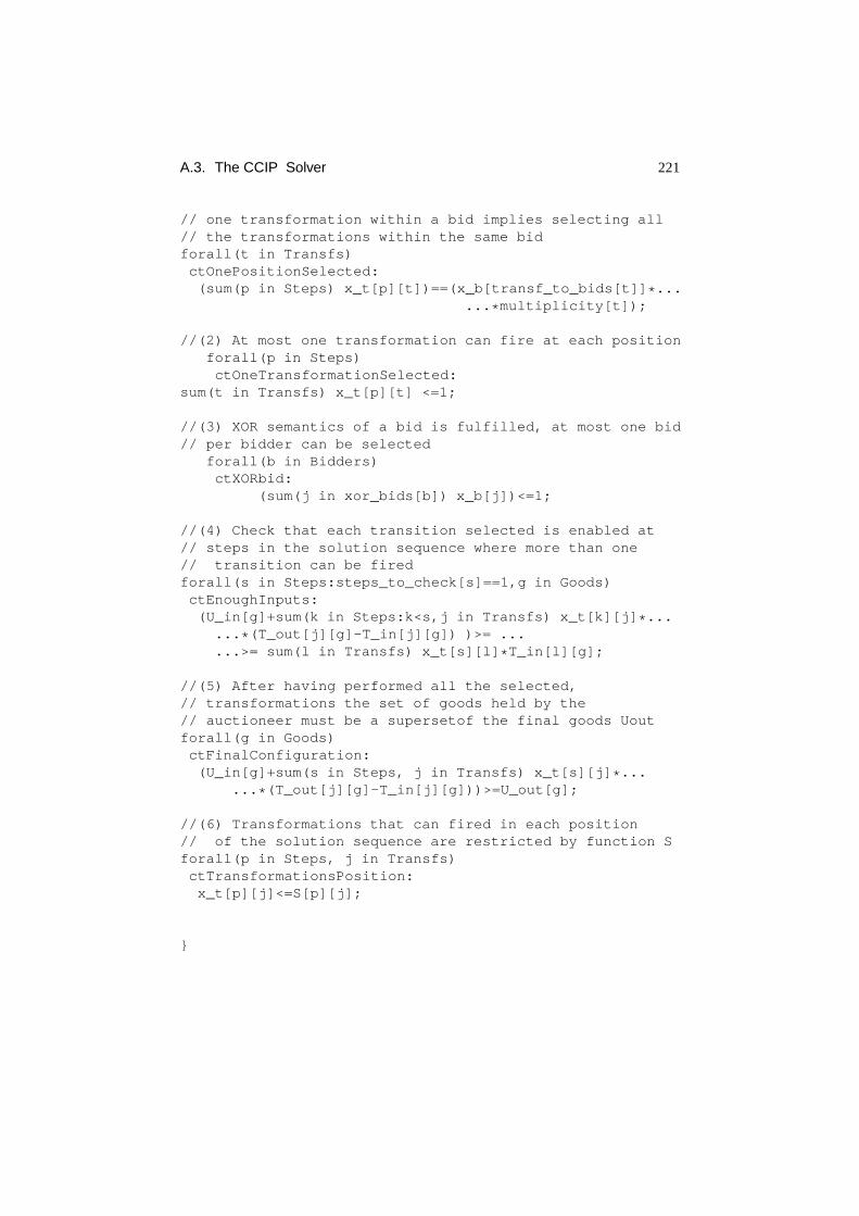
A.3. The CCIP Solver 221
// one transformation within a bid implies selecting all// the transformations within the same bidforall(t in Transfs)ctOnePositionSelected:(sum(p in Steps) x_t[p][t])==(x_b[transf_to_bids[t]]*...
...*multiplicity[t]);
//(2) At most one transformation can fire at each positionforall(p in Steps)ctOneTransformationSelected:
sum(t in Transfs) x_t[p][t] <=1;
//(3) XOR semantics of a bid is fulfilled, at most one bid// per bidder can be selected
forall(b in Bidders)ctXORbid:
(sum(j in xor_bids[b]) x_b[j])<=1;
//(4) Check that each transition selected is enabled at// steps in the solution sequence where more than one// transition can be firedforall(s in Steps:steps_to_check[s]==1,g in Goods)ctEnoughInputs:(U_in[g]+sum(k in Steps:k<s,j in Transfs) x_t[k][j]*...
...*(T_out[j][g]-T_in[j][g]) )>= ...
...>= sum(l in Transfs) x_t[s][l]*T_in[l][g];
//(5) After having performed all the selected,// transformations the set of goods held by the// auctioneer must be a supersetof the final goods Uoutforall(g in Goods)ctFinalConfiguration:(U_in[g]+sum(s in Steps, j in Transfs) x_t[s][j]*...
...*(T_out[j][g]-T_in[j][g]))>=U_out[g];
//(6) Transformations that can fired in each position// of the solution sequence are restricted by function Sforall(p in Steps, j in Transfs)ctTransformationsPosition:x_t[p][j]<=S[p][j];
}


Bibliography
Aissaoui, N., Haouari, M., and Hassini, E. (2007). Supplierselection and order lotsizing modeling: A review.Computers and Operations Research, 34(12):3516–3540.
Alonso-Ayuso, A., Escudero, L., Garın, A., Ortuno, M., and Perez, G. (2003). An Ap-proach for Strategic Supply Chain Planning under Uncertainty based on Stochastic0-1 Programming.Journal of Global Optimization, 26(1):97–124.
An, N., Elmaghraby, W., and Keskinocak, P. (2005). Bidding strategies and their impacton revenues in combinatorial auctions.Journal of Revenue and Pricing Manage-ment, 3(4):337–357(21).
Andersson, A., Tenhunen, M., and Ygge, F. (2000). Integer programming for com-binatorial auction winner determination. InFourth International Conference onMultiagent Systems (ICMAS 2000), pages 39–46, Boston, MA.
Ausubel, L. M., Cramton, P., and Milgrom, P. (2006).The Clock-Proxy Auction: APractical Combinatorial Auction Design, chapter 5. Combinatorial Auctions. MITPress.
Ausubel, L. M. and Milgrom, P. (2006a).Ascending Proxy Auctions, chapter 3. Com-binatorial Auctions. MIT Press.
Ausubel, L. M. and Milgrom, P. (2006b).The Lovely but Lonely Vickrey Auction, chap-ter 1. Combinatorial Auctions. MIT Press.
Babanov, A., Collins, J., and Gini, M. (2003). Asking the right question: Risk and ex-pectation in multiagent contracting.Artificial Intelligence For Engineering DesignAnalysis And Manufacturing, 17:173–186.
Ball, M. O., Donohue, G. L., and Hoffman, K. (2006).Auctions for the Safe, Efficient,and Equitable Allocation of Airspace System Resources, chapter 20. CombinatorialAuctions. MIT Press.
Banks, J., Ledyard, J., and Porter, D. (1989). Allocating Uncertain and Unrespon-sive Resources: An Experimental Approach.The RAND Journal of Economics,20(1):1–25.
223
224 BIBLIOGRAPHY
Bartels, A., Ragsdale, J., Pohlmann, T., Young, G. O., and Brown, K. (2005). Theforrester wave: e-sourcing suites, Q4 2005. Technical report, Forrester. TechNotes.
Bernardinello, L. and de Cindio, F. (1992). A survey of basicnet models and modularnet classes. InAdvances in Petri Nets 1992, The DEMON Project, pages 304–351,London, UK. Springer-Verlag.
Bichler, M., Davenport, A., Hohner, G., and Kalagnanam, J. (2006). Industrial Pro-curement Auctions, chapter 23. Combinatorial Auctions. MIT Press.
Blizard, W. and File, P. (1988). Multiset theory.Notre Dame J. Formal Logic, 30(1):36–66.
Blum, C. and Roli, A. (2003). Metaheuristics in combinatorial optimization: Overviewand conceptual comparison.ACM Computing Surveys (CSUR), 35(3):268–308.
Boutilier, C., Goldszmidt, M., and Sabata, B. (1999). Sequential Auctions for theAllocation of Resources with Complementarities.Proceedings of the SixteenthInternational Joint Conference on Artificial Intelligencetable of contents, pages527–523.
Boutilier, C. and Hoos, H. (2001). Bidding languages for combinatorial auctions.Proceedings of the 17th International Joint Conference on Artificial Intelligence,pages 1211–1217.
Burkeman, O. (5 september 2005). The wiki way. Guardian Unlimitedwww.guardian.co.uk/technology/2007/sep/05/news.netrich.
Cantillon, E. and Pesendorfer, M. (2006).Auctioning Bus Routes: The London Experi-ence, chapter 22. Combinatorial Auctions. MIT Press.
Caplice, C. and Sheffi, Y. (2006).Combinatorial Auctions for Truckload Transporta-tion, chapter 21. Combinatorial Auctions. MIT Press.
Christie’s (2007). Online.http://www.christies.com/.
Coase, R. (1937). The Nature of the Firm.Economica, 4(16):386–405.
Cohen, M. and Lee, H. (1988). Strategic Analysis of Integrated Production-DistributionSystems: Models and Methods.Operations Research, 36(2):216–228.
Collins, J. (2002).Solving Combinatorial Auctions with Temporal Constraintsin Eco-nomic Agents. PhD thesis, University Of Minnesota.
Corbett, M. (2004).The Outsourcing Revolution: Why it Makes Sense and how to Doit Right. Dearborn Trade Pub.
Cormen, T. (2001).Introduction to Algorithms. MIT Press.
Cramton, P. (2006).Simultaneous Ascending Auctions, chapter 4. Combinatorial Auc-tions. MIT Press.

BIBLIOGRAPHY 225
Cramton, P., Shoham, Y., and Steinberg, R., editors (2006).Combinatorial Auctions.MIT Press.
Davey, B. and Priestley, H. (2002).Introduction to Lattices and Order. CambridgeUniversity Press.
de Vries, S. and Vohra, R. (2003). Combinatorial auctions: Asurvey. INFORMSJournal of Computing, 15(3):284–309.
DMReview.com online news (March 22, 2006). Business outsourcing makes strongpush forward with small and midsize deals. Online News.
DMReview.com online news (October 31, 2005). Worldwide bpomarket steadily ex-pands. Online News.
Dyer, J. (2000).Collaborative Advantage: Winning Through Extended Enterprise Sup-plier Networks. Oxford University Press US.
Ebay (2007). Online.http://www.ebay.com.
Engel, Y., Wellman, M. P., and Lochner, K. M. (2006). Bid expressiveness and clearingalgorithms in multiattribute double auctions. InEC ’06: Proceedings of the 7thACM conference on Electronic commerce, pages 110–119, New York, NY, USA.ACM Press.
Erenguc, S., Simpson, N., and Vakharia, A. (1999). Integrated production/distributionplanning in supply chains: An invited review.European Journal of OperationalResearch, 115(2):219–236.
Ertogral, K., Wu, S., and Burke, L. (1998). Coordination Production and TransportationScheduling in the Supply Chain.Dept. IMSE, Lehigh Univ., Bethlehem, PA, Tech.Rep.
Esparza, J. and Melzer, S. (2004). Verification of safety properties using integer pro-gramming: Beyond the state equation.Formal Methods in System Design, 16:159–189.
Fourer, R., Gay, D., and Kernighan, B. (1989).AMPL: A Mathematical ProgrammingLanguage. AT&T Bell Laboratories.
Fujishima, Y., Leyton-Brown, K., and Shoham, Y. (1999). Taming the computationalcomplexity of combinatorial auctions: Optimal and approximate approaches. InProceeding of the Sixteenth International Joint Conference on Artificial Intelli-gence (IJCAI’99), pages 548–553.
Gaonkar, R. and Viswanadham, N. (2001). Collaboration and information sharing inglobal contractmanufacturing networks.Mechatronics, IEEE/ASME Transactionson, 6(4):366–376.
226 BIBLIOGRAPHY
Gaonkar, R. and Viswanadham, N. (2005). Strategic sourcingand collaborative plan-ning in Internet-enabled supply chain networks producing multigeneration prod-ucts. Automation Science and Engineering, IEEE Transactions on [see alsoRobotics and Automation, IEEE Transactions on], 2(1):54–66.
Greaver, M. (1999).Strategic Outsourcing: A Structured Approach to OutsourcingDecisions and Initiative. AMACOM.
Hammer, M. (2001). The Superefficient Company.Harvard Business Review,79(8):82–91.
Harary, F. (1999).Graph Theory. Perseus Books.
He, M., Jennings, N., and Leung, H. (2003). On agent-mediated electronic commerce.IEEE Transactions on Knowledge and Data Engineering, 15(4):985–1003.
Hillier, F. and Lieberman, G. (1986).Introduction to Operation Research. McGraw-Hill.
Holte, R. C. (2001). Combinatorial auctions, knapsack problems, and hill-climbingsearch. InLecture Notes in Computer Science, volume 2056, pages 57 – 66.Springer-Verlag, Heidelberg.
ILOG (2007). Cplex.http://www.ilog.com/products/cplex/.
Jayaraman, V. and Pirkul, H. (2001). Planning and coordination of production anddistribution facilities for multiple commodities.European Journal of OperationalResearch, 133(2):394–408.
Jennings, N. and Wooldridge, M. (1998). Applications of intelligent agents.Agenttechnology: foundations, applications, and markets tableof contents, pages 3–28.
Kalagnanam, J. and Parkes, D. (2003). Auctions, Bidding andExchange Design. Chap-ter 10.Supply Chain Analysis in the eBusiness Era. Edited by David Simchi-Levi,S. David Wu and Z. Max Shen.
Kallrath, J. (2002). Planning and scheduling in the processindustry. OR Spectrum,24(3):219–250.
Kallrath, J. (2004).Modeling Languages in Mathematical Optimization. Kluwer Aca-demic Pub.
Kellerer, H., Pferschy, U., and Pisinger, D. (2004).Knapsack problems. Springer NewYork.
Klemperer, P. (2004).Auctions: Theory and Practice. Princeton University Press.
Krishna, V. (2002).Auction Theory. Academic Press.
Land, A., Powell, S., and Steinberg, R. (2006).PAUSE: A Computationally TractableCombinatorial Auction, chapter 6. Combinatorial Auctions. MIT Press.
BIBLIOGRAPHY 227
Lau, J., Huang, G., Mak, K., and Liang, L. (2006). Agent-based modeling of supplychains for distributed scheduling.Systems, Man and Cybernetics, Part A, IEEETransactions on, 36(5):847 – 861.
Laubacher, R. and Malone, T. (2003). Retreat of the Firm and the Rise of the Guilds:The Employment Relationship in an Age of Virtual Business.Inventing the Or-ganization of the 21st Century. Malone TW, Laubacher R, Scott-Morton MS (eds).MIT Press.
Lee, Y., Jeong, C., and Moon, C. (2002). Advanced planning and scheduling withoutsourcing in manufacturing supply chain.Computers & Industrial Engineering,43(1-2):351–374.
Lee, Y., Kumara, S., and Chatterjee, K. (2003). Multiagent based dynamic resourcescheduling for distributed multiple projects using a market mechanism.Journal ofIntelligent Manufacturing, 14(5):471–484.
Lehmann, D., Mueller, R., and Sandholm, T. M. (2006).The winner determinationproblem, chapter 12. Combinatorial Auctions. MIT Press.
Leyton-Brown, K. and Shoham, Y. (2006).Combinatorial Auctions, chapter 18. A TestSuite for Combinatorial Auctions. MIT Press.
Leyton-Brown, K., Shoham, Y., and Tennenholtz, M. (2000). An algorithm for multi-unit combinatorial auctions. InProceedings of the American Association for Arti-ficial Intelligence Conference (AAAI), pages 56–61.
Lih, A. (2003). Wikipedia as Participatory Journalism: Reliable Sources? Metrics forevaluating collaborative media as a news resource.Nature, 2004.
Lindo Systems Inc. (2007). Lingo.http://www.lindo.com/products/lingo.
Lipton, R. (1976). The reachability problem requires exponential space. TechnicalReport 62, Yale University.
Lucking-Reiley, D. and Spulber, D. (2001). Business-to-Business Electronic Com-merce.The Journal of Economic Perspectives, 15(1):55–68.
Makhorin, A. GNU Linear Programming Kit: Modelling Language GNU MathProg.
Makhorin, A. (2001). Glpk – gnu linear programming toolkit.http://www.gnu.org/directory/GNU/glpk.html. [Online; ac-cessed 25-Oct-2007].
Mas-Colell, A., Whinston, M., and Green, J. (1995).Microeconomic Theory. OxfordUniversity Press.
McAfee, R. and McMillan, J. (1987). Auctions and Bidding.Journal of EconomicLiterature, 25(2):699–738.
Microsoft (2007). Excel.http://office.microsoft.com/en-us/excel/.

228 BIBLIOGRAPHY
Milgrom, P. (2004).Putting Auction Theory to Work. Cambridge University Press.
Minahan, T., Howarth, F., and Vigoroso, M. (2002). Making e–sourcing strategic.Re-search report, Aberdeen Group, Boston.
Mowshowitz, A. (2002).Virtual Organization: Toward a Theory of Societal Transfor-mation Stimulated by Information Technology. Quorum/Greenwood.
Muller, R. (2006).Tractable Cases of the Winner Determination Problem, chapter 13.Combinatorial Auctions. MIT Press.
Murata, T. (1989). Petri nets: Properties, analysis and applications. InIEEE, volume 77,pages 541–580.
Nisan, N. (2000). Bidding and allocation in combinatorial auctions. InProc. 2nd ACMConference on Electronic Commerce (EC-2000). ACM Press.
Nisan, N. (2006).Bidding Languages for Combinatorial Auctions, chapter 9. Combi-natorial Auctions. MIT Press.
Norman, T., Preece, A., Chalmers, S., Jennings, N., Luck, M., Dang, V., Nguyen, T.,Deora, V., Shao, J., Gray, W., et al. (2004). Agent-based formation of virtualorganisations.Knowledge-Based Systems, 17(2-4):103–111.
Ottens, B. (2007). Comparing winner determination algorithms for mixed multi-unitcombinatorial auctions. Master’s thesis, Universiteit van Amsterdam., Nether-lands.
Papadimitriou, C. and Steiglitz, K. (1982).Combinatorial optimization: algorithmsand complexity. Prentice-Hall, Inc. Upper Saddle River, NJ, USA.
Parkes, D. C. (2006).Iterative Combinatorial Auctions, chapter 2. Combinatorial Auc-tions. MIT Press.
Pekec, A. and Rothkopf, M. H. (2003). Combinatorial auctiondesign. Manage. Sci.,49(11):1485–1503.
Petri, C. (1962).Kommunikation mit Automaten. PhD thesis, Rheinisch-WestfalischesInstitut f. instrumentelle Mathematik an d. Univ.
Petri, C. (1966). Kommunikation mit automaten. Schriften des iim nr. 2, Institut furInstrumentelle Mathematic, 1962. Technical report, English translation: TechnicalReport RADC-TR-65-377, Griffiths Air Base, New York.
Quinn, J. and Hillmer, F. (1995). Strategic Outsourcing.The McKinsey Quarterly, (1).
Reis, J., Mamede, N., and O Neill, H. (2001). Locally perceiving hard global constraintsin multi-agent scheduling.Journal of Intelligent Manufacturing, 12(2):223–236.
Reisig, W. (1985).Petri nets: an introduction. Springer-Verlag, New York, NY, USA.
BIBLIOGRAPHY 229
Reyes-Moro, A., Rodrıguez-Aguilar, J. A., Lopez-Sanchez, M., Cerquides, J., andGutierrez-Magallanes, D. (2003). Embedding decision support in e-sourcing tools:Quotes, a case study.Group Decision and Negotiation, 12:347–355.
Rosenschein, J. and Zlotkin, G. (1994).Rules of encounter. MIT Press Cambridge,Mass.
Rothkopf, M. H., Pekec, A., and Harstad, R. M. (1998). Computationally manageablecombinational auctions.Management Science, 44(8):1131–1147.
Sabri, E. and Beamon, B. (2000). A multi-objective approachto simultaneous strategicand operational planning in supply chain design.Omega, 28(5):581–598.
Sandholm, T. (2002). Algorithm for optimal winner determination in combinatorialauctions.Artificial Intelligence, 135(1-2):1–54.
Sandholm, T. (2006a). Expressive commerce and its application to sourcing.Proceed-ings of the Innovative Applications of Artificial Intelligence.
Sandholm, T. (2006b).Optimal Winner Determination Algorithms, chapter 14. Combi-natorial Auctions. MIT Press.
Sandholm, T., Suri, S., Gilpin, A., and Levine, D. (2002). Winner determination incombinatorial auction generalizations. InAAMAS ’02: Proceedings of the first in-ternational joint conference on Autonomous agents and multiagent systems, pages69–76, Bologna, Italy. ACM Press.
Schrage, M. (2007). The Myth of Commoditization.Sloan management review,48(2):10–14.
Shaeffer, L. D. (September 11, 2007). Five More Keys to Engaging the Customer toProduce Real Innovation: Lessons From LEGO.
Simchi-Levi, D., Kaminsky, P., and Simchi-Levi, E. (2000).Designing and Managingthe Supply Chain: Concepts, Strategies, and Case Studies. Irwin/McGraw-Hill.
Smith, R. (1980). The Contract Net Protocol: High-Level Communication and Controlin a Distributed Problem Solver.IEEE Transactions on Computers, 29(12):1104–1113.
Sotheby’s (2007). Online.http://www.sothebys.com/.
SourceForge, S.F. (2007). SourceForge.net Home Page.http://www.sourceforge.net.
Syropoulos, A. Mathematics of Multisets.Pre-proceedings of the Workshop on MultisetProcessing, pages 286–295.
Tapscott, D. and Williams, A. (2006).Wikinomics: how mass collaboration changeseverything. Portfolio.

230 BIBLIOGRAPHY
Tarek, A. and Lopez-Benitez, N. (2004). Optimal legal firingsequence of petri netsusing linear programming.Optimization and Engineering, 5(1):25–43.
Team, I. S. C. (2001). Strategic sourcing: Applications to turn direct materials pro-curement into competitive advantage. Technical report, Stephens Inc. IndustryReport.
Van Hentenryck, P. (1999).The OPL optimization programming language. MIT PressCambridge, MA, USA.
Vinyals, M. (2007a). Bid generator figures. Internal Communication.
Vinyals, M. (2007b). On the empirical evaluation of mixed multi-unit combinatorialauctions. Master’s thesis, Universitat Autonoma de Barcelona.
Vinyals, M., Cerquides, J., and Rodriguez-Aguilar, J. A. (2007a). On the empirical eval-uation of mixed multi-unit combinatorial auctions.Workshop on Agent MediatedElectronic Commerce IX,AMEC.
Vinyals, M., Giovannucci, A., Cerquides, J., Meseguer, P.,and Rodriguez-Aguilar, J. A.(2007b). Towards a realistic bid generator for mixed multi-unit combinatorialauctions. 14th Workshop on Experimental Evaluation of Algorithms forSolvingProblems with Combinatorial Explosion RCRA.
Viswanadham, N. (2002). The past, present, and future of supply-chain automation.IEEE Robotics & Automation Magazine, 9(2):48–56.
Wagner, T., Guralnik, V., and Phelps, J. (2003). TAEMS agents: enabling dynamicdistributed supply chain management.Electronic Commerce Research and Appli-cations, 2(2):114–132.
Walsh, W. and Wellman, M. (2003). Decentralized supply chain formation: A marketprotocol and competitive equilibrium analysis.Journal of Artificial IntelligenceResearch, 19:513–567.
Walsh, W. E. (2001).Market protocols for decentralized supply chain formation. PhDthesis. Chair-Michael P. Wellman.
Walsh, W. E., Wellman, M. P., and Ygge, F. (2000). Combinatorial auctions for supplychain formation. InProc. of the 2nd ACM Conference on Electronic Commerce.
Wooldridge, M. and Jennings, N. (1995). Intelligent Agents: Theory and Practice.Knowledge Engineering Review, 10(2):115–152.
Wurman, P., Walsh, W., and Wellman, M. (1998). Flexible double auctions for elec-tionic commerce: Theory and implementation.Decision Support Systems, 24:17–27.
Zhang, X. (2002).Sophisticated Negotiation in Multi-agent Systems. PhD thesis, Uni-versity of Massachusetts at Amherst.

BIBLIOGRAPHY 231
Zlotkin, G. and Rosenschein, J. (1996). Mechanism design for automated negotiation,and its application to task oriented domains.Artificial Intelligence, 86(2):195–244.


Monografies de l’Institut d’Investigaci o enIntel ·ligencia Artificial
Num. 1 J. Puyol,MILORD II: A Language for Knowledge–Based Systems,(1995).
Num. 2 J. Levy,The Calculus of Refinements, a Formal Specification ModelBased on Inclusions, (1995).
Num. 3 Ll. Vila, On Temporal Representation and Reasoning in Knowledge–Based Systems, (1995).
Num. 4 M. Domingo,An Expert System Architecture for Identification in Bi-ology, (1995).
Num. 5 E. Armengol,A Framework for Integrating Learning and ProblemSolving, (1998).
Num. 6 J. Ll. Arcos,The Noos Representation Language, (1998).Num. 7 J. Larrosa,Algorithms and Heuristics for Total and Partial Constraint
Satisfaction, (1998).Num. 8 P. Noriega,Agent Mediated Auctions: The Fishmarket Metaphor,
(1999).Num. 9 F. Manya,Proof Procedures for Multiple-Valued Propositional Log-
ics, (1999).Num. 10 W. M. Schorlemmer,On Specifying and Reasoning with Special Re-
lations, (1999).Num. 11 M. Lopez-Sanchez,Approaches to Map Generation by means of Col-
laborative Autonomous Robots, (2000).Num. 12 D. Robertson,Pragmatics in the Synthesis of Logic Programs, (2000).Num. 13 P. Faratin,Automated Service Negotiation between Autonomous Com-
putational Agents, (2003).Num. 14 J. A. Rodrıguez,On the Design and Construction of Agent-mediated
Electronis Institutions, (2003).Num. 15 T. Alsinet,Logic Programming with Fuzzy Unification and Imprecise
Constants: Possibilistic Semantics and Automated Deduction, (2003).Num. 16 A. Zapico,On Axiomatic Foundations for Qualitative Decision The-
ory - A Possibilistic Approach, (2003).Num. 17 A. Valls,ClusDM: A multiple criteria decision method for heteroge-
neous data sets, (2003).Num. 18 D. Busquets,A Multiagent Approach to Qualitative Navigation in
Robotics, (2003).Num. 19 M. Esteva,Electronic Institutions: from specification to development,
(2003).Num. 20 J. Sabater,ReGreT, a trust and reputation model for multi-agent sys-
tems, (2003).

Num. 21 J. Cerquides,Improving Algorithms for Learning Bayesian NetworkClassifiers, (2005).
Num. 22 M. Villaret,On Some Variants of Second-Order Unification, (2005).Num. 23 M. Gomez,Open, Reusable and Configurable Multi-Agent Systems:
A Knowledge Modelling Approach, (2005).Num. 24 S. Ramchurn,Multi-Agent Negotiation Using Trust and Persuasion,
(2005).Num. 25 S. Ontanon,Ensemble Case-Based Learning for Multi-Agent Systems,
(2006).Num. 26 M. Sanchez,Contributions to Search and Inference Algorithms for
CSP and Weighted CSP, (2006).Num. 27 C. Noguera,Algebraic Study of Axiomatic Extensions of Triangular
Norm Based Fuzzy Logics, (2007).Num. 28 E. Marchioni,Functional Definability Issues in Logics Based on Tri-
angular Norms, (2007).Num. 29 M. Grachten,Expressivity-Aware Tempo Transformations of Music
Performances Using Case Based Reasoning, (2007).Num. 30 I. Brito,Distributed Constraint Satisfaction, (2007).Num. 31 E. Altamirano,On Non-clausal Horn-like Satisfiability Problems,
(2007).Num. 32 A. Giovannucci,Computationally Manageable Combinatorial Auc-
tions for Supply Chain Automation, (2008).
