32. marine outfalls

Marine Outfa7

PartC|32

32. Marine Outfalls

Peter M. Tate, Salvatore Scaturro, Bruce Cathers

Marine outfalls are used to discharge treated liquidwaste to the environment. Not all contaminants inliquid waste can be removed by treatment. A prop-erly designed, constructed, and operated marineoutfall effectively dilutes the discharged wastewhich then substantially reduces the concentra-tion of contaminants in the wastewater. In turn,this reduces the risk to biota and human users ofthe marine environment. An introduction to someof the main aspects of marine outfalls is provided.

Five areas are covered, commencing with themain influences associated with the decision tobuild a marine outfall. Included is an overviewof the wastewater treatment process. Near-fieldnumerical modeling is described and it is demon-strated how this tool can be used to assist withthe design of a marine outfall. Outfall hydraulicsis discussed, detailing a range of features includ-ing head losses, manifolds (or diffusers), seawaterintrusion, and air entrainment. A very brief sum-mary of the construction of a marine outfall isprovided. The final area covered describes envi-ronmental monitoring that should be undertakento confirm the putative impacts associated witha marine outfall.

32.1 Terminology .......................................... 8

32.2 Governance . .......................................... 932.2.1 Drivers for a Marine Outfall .......... 932.2.2 Wastewater Treatment ................. 10

32.2.3 Data Collectionfor Outfall Design ........................ 11

32.3 Predicting Near-Field Dilutions .............. 1232.3.1 Physical Models........................... 1332.3.2 Positively Buoyant Jets

and Plumes ................................ 1332.3.3 Negatively Buoyant Jets ............... 1432.3.4 Model Validation ......................... 1432.3.5 Far-Field Numerical Modeling ...... 1732.3.6 Data for Running the Models ........ 1732.3.7 Conceptual Design

for Positively BuoyantDischarges .................................. 18

32.4 Hydraulic Analysis and Design ................ 1932.4.1 Governing Hydraulics ................... 1932.4.2 Diffusers – Hydraulic Design ......... 2132.4.3 Flow Variability ........................... 2532.4.4 Hydraulic Integration ................... 2632.4.5 Air Entrainment........................... 2832.4.6 Sedimentation ............................ 29

32.5 Outfall Construction . .............................. 3032.5.1 Construction Materials ................ 3032.5.2 Construction Methods ................. 3032.5.3 Some Considerations ................... 31

32.6 Environmental Monitoring ..................... 3232.6.1 Change Versus Impact . ................. 3232.6.2 Pre- and Postconstruction

Monitoring ................................. 3232.6.3 Long-Term Monitoring ................. 3432.6.4 Summary .................................... 35

References ..................................................... 35

Work presented in this chapter concentrates on thedischarge of wastewater to the environment throughmarine outfalls. Marine structures are required for in-takes for drinking water (e.g., desalination plants) andwater for industrial or commercial use (e.g., flushing oftoilets). The focus here is on marine outfalls; marine in-takes are not considered further.The objective here is to provide practitioners with anoverview of the fundamentals of marine outfalls and to

outline some initial considerations to help those newto the subject area. Understandably, the present chap-ter does not cover all areas in detail; the focus is on thedesign and monitoring aspects of marine outfalls. Infor-mation on some of the problems drawn from experiencewith marine outfalls is provided and reference materialwith additional detail is identified.

PartC|32.1

8 Part C Coastal Design

32.1 Terminology

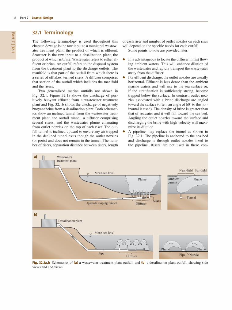
The following terminology is used throughout thischapter. Sewage is the raw input to a municipal wastew-ater treatment plant, the product of which is effluent.Seawater is the raw input to a desalination plant, theproduct of which is brine. Wastewater refers to either ef-fluent or brine. An outfall refers to the disposal systemfrom the treatment plant to the discharge outlets. Themanifold is that part of the outfall from which there isa series of offtakes, termed risers. A diffuser comprisesthat section of the outfall which includes the manifoldand the risers.

Two generalized marine outfalls are shown inFig. 32.1. Figure 32.1a shows the discharge of pos-itively buoyant effluent from a wastewater treatmentplant and Fig. 32.1b shows the discharge of negativelybuoyant brine from a desalination plant. Both schemat-ics show an inclined tunnel from the wastewater treat-ment plant, the outfall tunnel, a diffuser comprisingseveral risers, and the wastewater plume emanatingfrom outlet nozzles on the top of each riser. The out-fall tunnel is inclined upward to ensure any air trappedin the declined tunnel exits though the outlet nozzles(or ports) and does not remain in the tunnel. The num-ber of risers, separation distance between risers, length

a)

b)

Wastewatertreatment plant

Desalination plant

Ambientcurrent

Mean sea levelNear-field

Tunnel

Plume

Pipe Nozzle

Plume

RisersDiffuser

DiffuserPipe

Upwards sloping tunnel

Far-field

Plume Plume

Mean sea level

Fig. 32.1a,b Schematics of (a) a wastewater treatment plant outfall, and (b) a desalination plant outfall, showing sideviews and end views

of each riser and number of outlet nozzles on each riserwill depend on the specific needs for each outfall.

Some points to note are provided later:

� It is advantageous to locate the diffuser in fast flow-ing ambient waters. This will enhance dilution ofthe wastewater and rapidly transport the wastewateraway from the diffuser.� For effluent discharge, the outlet nozzles are usuallyhorizontal. Effluent is less dense than the ambientmarine waters and will rise to the sea surface or,if the stratification is sufficiently strong, becometrapped below the surface. In contrast, outlet noz-zles associated with a brine discharge are angledtoward the surface (often, an angle of 60° to the hor-izontal is used). The density of brine is greater thanthat of seawater and it will fall toward the sea bed.Angling the outlet nozzles toward the surface anddischarging the brine with high velocity will maxi-mize its dilution.� A pipeline may replace the tunnel as shown inFig. 32.1. The pipeline is anchored to the sea bedand discharge is through outlet nozzles fixed tothe pipeline. Risers are not used in these con-

Marine Outfalls 32.2 Governance 9Part

C|32.2

figurations. (Risers are vertical structures used totransfer the wastewater from an outfall tunnel tothe outlet nozzles. They may be tens of metres inlength).� The number of outlet nozzles attached to each riseris usually restricted to eight or less. If more thaneight outlet nozzles are used, the plumes from ad-jacent nozzles interfere with each other and reducethe effective dilution of the wastewater.� The outfall pipeline and diffuser may be tapered toensure the velocity of the wastewater remains suf-

ficiently high to prevent sediments from settling inthe pipeline.� Outlet nozzles may be fitted with nonreturn checkvalves (also called duckbill valves). These valvesare closed when the wastewater flow is zero and pre-vent the ingress of seawater into the pipeline. Oneadvantage of check valves is that they enhance di-lution, compared with a round nozzle of the samecross-sectional area [32.1]. However, they may befouled by biota or fishing nets, rendering them per-manently open or closed.

32.2 Governance

There are many factors affecting the decision to builda marine outfall.

Municipal wastewater collects at the bottom of thecatchment. For a coastal city, this is at the edge of themarine environment. There are large costs associatedwith the movement of wastewater to the top of a catch-ment for potable reuse, including construction of a pipenetwork, pumps, and energy required to operate thepumps. Furthermore, there may be high costs associatedwith the conversion of wastewater to potable water. Thedisposal of wastewater through a marine outfall maybe the best overall use of resources. Despite this, thedecision to proceed with a marine outfall should firstexamine other options and maximize the beneficial usesof recycled wastewater.

32.2.1 Drivers for a Marine Outfall

SPHERE is an acronym we use to describe the mainfactors overlying the need for government sponsoreddevelopment (social, public health, environmental, reg-ulation, economic). The first three elements of SPHERErepresent the main aspects in which a marine out-fall has an impact (i. e., the community values). Thelast two elements of SPHERE represent the con-straints on the marine outfall – regulation tendingtoward high treatment and consequential high cost andeconomic tending toward low cost and consequentiallow treatment. Below, some of the considerations ofSPHERE are described in the context of a marineoutfall.

Most countries have environmental guidelines thatneed to be met during the design of a marine outfall.These guidelines are unique to each country and all can-not be detailed here. Suffice to say that they includemeeting concentrations of contaminants which may in-clude pathogens, nutrients, metals, and organics. Theseguidelines usually apply at the boundary of a mixing

zone, which needs to be clearly defined prior to con-struction of the marine outfall.

SocialWhat does the community expect from a marine out-fall? What are the values that are important to thecommunity? This will vary among and within differentgeographical regions and cultural groups. Some com-munities will comprise a large number of beach users.To them, the concept of a marine outfall may not bepalatable unless it can be clearly demonstrated that themarine outfall poses minimal risk to their use of the ma-rine environment.

Public HealthIs it safe to swim in the marine waters? What are thetypes and concentrations of substances that will be dis-charged to the marine environment? Will they be ofharm to us? Much information is available to informus about of the potential harm of substances that maybe discharged through a marine outfall. Most countriessynthesize this information into a set of guidelines ap-plicable to their marine environment. There is a tacitassumption that, provided the concentrations of the sub-stances are kept below harmful levels, the health of theusers of the marine environment will be maintained.This does require knowledge of the types, concentra-tions, and variability of the substances in the wastew-ater. It should be noted here that all the substances arepotentially toxic given sufficiently high concentrationsand the environment into which they are discharged.

EnvironmentalWill the discharge of substances through the marineoutfall cause harm to marine organisms? Will the ma-rine environment be degraded into the future? Will thebeaches and marine waters be free from visible pol-lution – oil, grease, rags, etc.? As noted under Public

PartC|32.2


Health, most countries have environmental guidelines.Provided these guidelines are met, it is assumed that themarine environment will be protected. The guidelinesare usually in the form of concentrations of substances(e.g., metals, nutrients, and bacteria) that should be metat a specific distance from the outfall (this distance de-fines a mixing zone). This implies that there will bea region inside the mixing zone in which the guidelinesmay not be met. The consequences are that the biologi-cal diversity inside the mixing zone may not be the sameas that in reference areas.

RegulationWhat are the regulations that govern the discharge ofany substance to the marine environment? Regulationsare often in the form of licence conditions restrictingthe types, concentrations, and/or loads of substancesthat can be discharged to the marine environment. Asnoted above, there is a tacit assumption that keepingwithin these restrictions will ensure the safety of hu-mans, and the protection of flora and fauna in the marineenvironment.

EconomicGovernments will invest a large amount of money forthe construction of a marine outfall. Ultimately, thismoney is raised through taxes and governments are ac-countable for the wise use of the taxes they collect.Outfall dollars will be competing with funding areas asdiverse as education, security, and care for the aged.What does the community value? What is the com-munity willing to pay to protect both humans and theenvironment? The marine outfall is just one of manyoptions that should be considered. Ultimately there isa balance between the level of protection offered andthe cost incurred by each option. It is the responsibil-ity of the engineer and scientist to evaluate each optionand provide the government with the most effectivesolution.

32.2.2 Wastewater Treatment

Our main focus in this section is on municipal outfalls.Critical to a marine outfall is knowledge of what is be-ing discharged, particularly the types, concentrations,and variability of contaminants in the wastewater. Dis-charge of contaminants from other sources includingprivate outfalls, rivers and estuaries, atmospheric in-puts, discharges from vessels, and illegal dumping arenot considered. The reader is referred to Tchobanoglouset al. [32.2], which provides considerable detail onwastewater treatment.

Wastewater discharges from domestic, commercial,and industrial sources. Often, the wastewater systems

are not isolated from the environment and infiltrationof water during storms may also occur. The composi-tion of wastewater depends on the relative contributionof these three main sources and on the type and sizeof industry and/or commercial activity. Each wastewa-ter system is unique and treatment plants are designedto deal with the quantity and quality of wastewater pro-duced by a specific system.

Wastewater comprises particulate matter, patho-gens, nutrients, organic, and inorganic material. Severeenvironmental damage can result if wastewater is dis-charged undiluted or without treatment. Therefore themain objective of sewage treatment is the eliminationor reduction in concentration of these materials.

Different concentrations of substances will invokedifferent responses in different species. Metals may beadsorbed onto particulates that may be ingested by fishand shellfish. Organics are often adsorbed by the fattytissues in aquatic animals. Reducing the concentrationsof suspended solids, oil, and grease during the wastew-ater treatment process, reduces the quantity of metalsand organics that may affect marine organisms.

Wastewater treatment can be broadly divided intothree levels: primary, secondary and tertiary (or ad-vanced). The levels are modular, subsequent treatmentsbeing bolted onto lower levels of treatment. Withineach level of treatment there are multiple options thatproduce wastewater of similar quality. The distinc-tion among the treatment levels themselves is blurredand will depend on how individual levels are operatedand maintained. Usually, concentrations of suspendedsolids, biochemical oxygen demand (BOD), and indi-cator bacteria in the effluent are used to distinguish thelevels of treatment. The type of wastewater treatmentplant adopted is often based on the collective experi-ence of the engineers and process workers within anorganization.

Primary TreatmentPrimary treatment removes debris that could damagethe wastewater treatment system. This is done by pass-ing the sewage through trash racks and screens. Sewagethen flows through sedimentation tanks at low veloci-ties ensuring residence times of 2�3 h or more [32.2].This allows sufficient time for negatively buoyant solidsto settle at the bottom of the tank and positively buoy-ant oils and greases to rise to the surface of the tank.Chemicals can be added to the sewage to accelerate thesettling process. Both the solids and oil and grease canthen be easily removed. Primary treatment also helpsregulate the flow of sewage to subsequent levels oftreatment. Primary treatment may be used in isolation,but this usually depends on the environment into whichthe wastewater is discharged.

Marine Outfalls 32.2 Governance 11Part

C|32.2

Table 32.1 Median concentrations of substances in sewage and after various levels of treatment. The numbers are indica-tive only and may vary in time and between sewage treatment plants

Substance Units Raw sewage Primary Secondary TertiaryFaecal coliforms cfu=100 ml 107 106 104 10Suspended solids mg=l 250 100 10 < 5BOD mg=l 200 100 10 < 5Oil and grease mg=l 50 20 < 5 < 5Total nitrogen mg=l 50 40 20 10Total phosphorus mg=l 10 7 5 3

Secondary TreatmentSecondary treatment covers a wide range of biologicalprocesses including: activated sludge, trickling filters,rotating biological contactors, aerated lagoons, oxidiz-ing beds, and membrane bioreactors. The basic objec-tive of all of these processes is the removal of organicmaterial and suspended solids. Secondary treatmentmay also include disinfection to reduce the concentra-tions of bacteria in the wastewater. A common formof secondary treatment is activated sludge in whichmicroorganisms are mixed with the wastewater underaerobic conditions for about 4�8 h. The microorgan-isms metabolize the organic matter in the wastewater,ultimately producing inorganic materials.

Tertiary TreatmentTertiary treatment often involves the further removal ofsuspended materials using sand filters. High levels ofnitrogen and phosphorus may remain in the wastewa-ter after secondary treatment, which can contribute toexcessive primary production and eutrophication. Thebasic premise for nitrogen removal is to convert nitrateto nitrogen gas, which is then discharged to the atmo-sphere. Biological processes and chemical precipitationare two methods used to remove phosphorus from thewastewater. Once removed, phosphate can be used asa fertilizer.

Microfiltration and reverse osmosis are specificforms of advanced wastewater treatment. The wastew-ater is forced through a fine membrane. The size of themembrane mesh is sufficient to allow the passage of wa-ter, but larger materials are captured and removed fromthe wastewater. Increasingly, micro- or milli-filtrationare added to primary or secondary treatment processes.When combined with an effective outfall diffuser, thediluted wastewater may achieve licence requirements.

An indication of the median effluent concentrationsof selected substances after treatment is given in Ta-ble 32.1. It is stressed that these are general values thatwill differ for specific wastewater treatment plants andare highly variable.

A desalination plant discharges brine in which theprimary contaminant is salt. Median concentrations of

brine are about 60 psu, although it may vary between 40and 80 psu. The median salt content in seawater is about35 psu. Marine organisms can tolerate salt concentra-tions to about 39 psu [32.3], although this value varieswith different organisms. Therefore, the configurationof an outfall discharging brine to the marine environ-ment should ensure a rapid reduction in salinity to lessthan 39 psu.

32.2.3 Data Collection for Outfall Design

While the preliminary design of a marine outfall canbe undertaken using minimum data, the detailed designusually requires considerable data. The main aim forthese data collection programs is identification of thesite (or sites) for the marine outfall. That is, for the low-est cost, identifying the level of treatment and site thatbest meets the environmental (and other) guidelines.

The type and volume of data required dependson the marine outfall being considered. Broadly, datainclude: volume and flow rates of effluent to be dis-charged, water quality (both in the treated effluent andin the marine waters), ocean currents, and stratification.A critical aspect of monitoring, often overlooked, is thevariability of these data. Our favored approach is to usethe data variability in a Monte Carlo approach, runningthe models for many different combinations of inputvalues. This results in a statistical distribution of theconcentrations of contaminants in the marine waters,which can be synthesized in, for example, a probabil-ity of exceedance plot.

Historical data or data collected from differentprojects can be used. The difference between the dataneeds and the historical data defines a gap that a datacollection program needs to fill. Much of the data col-lected as part of these studies can also be used inSect. 32.6. Some of the main data collection programsare outlined below.

The volume of effluent flow can be estimated fromhuman population projections. This information allowsassessment of when environmental guidelines are likelyto be exceeded; hence when upgrades of the treatmentplant are likely to be needed.

PartC|32.3


Water quality in the treated effluent will be a func-tion of the level of treatment. Estimates can be obtainedfrom other, similar treatment plants or from the indica-tive values provided in Table 32.1. Ongoing monitoringof the effluent quality after construction will help ensuremaintenance of environmental standards.

Measuring water quality in the marine waters (intowhich the wastewater is discharged) provides back-ground concentrations of contaminants. The back-ground concentrations must be added to the modeledconcentrations to estimate the total concentration ofcontaminants in the marine waters. Background con-centrations may already exceed environmental guide-lines, in which case, they made need to be relaxedor another outfall location sought. To obtain a rep-resentative picture of marine water quality, samplingshould take place over large spatial and temporal scalesand should include replication. Instruments that can bemoored in the field for long periods of time are increas-ingly being used to obtain water quality measurements,although the accuracy of such results is less than can beachieved in the laboratory.

Current speed and direction are important for plumedilution. Moored current meters can provide detailedtemporal information at a point in space (or a pro-file throughout the water column). However, they areexpensive to deploy, maintain and retrieve, and care-ful consideration needs to be made in regard to thenumber and location of such moorings. Spatial in-formation can be obtained by profiling currents froma vessel underway, drifters drogued at specific depths

and remotely sensed data (e.g., via satellites or airbornescanners). The number and duration of moored cur-rent meters will depend on the size of the outfall underconsideration. For a moderately sized outfall, a sin-gle profiling current meter moored for 12 months andserviced monthly, provides the minimum data require-ments. A roving current meter (deployed at differentlocations for one month at a time) may provide a com-promise between the number of instruments and spatialcoverage.

Density stratification of the water column largelygoverns the height of rise of the wastewater. (The ef-fect is much reduced for brine discharges). In coastalmarine waters, density is a function of both tempera-ture and salinity, both of which should be measured. Forshallow outfalls (outfalls in water depths less than about10 m), stratification has little effect. However, for out-falls in deep waters, relatively small stratification mayproduce a submerged plume resulting in lower dilutionsand a nonvisible plume (at least to a surface observer).Moored temperature/salinity strings provide a profileof density throughout the water column, although ma-rine fouling will reduce the quality of data from salinitysensors. Such data can also be collected during the ser-vicing of moored instruments, which may be monthlyover a period of 12 months.

Other data such as surface waves and tides may alsobe important, particularly for shallow outfalls wherethe changes in water depth resulting from such pro-cesses may represent a significant proportion of thewater column.

32.3 Predicting Near-Field Dilutions

The design of a marine outfall centers on the dilutionrequired to meet the relevant guidelines. Occasionally,guidelines may be met after an appropriate level ofsewage treatment. However, many substances will relyon the dilution with marine waters to meet these guide-lines. Dilution depends on:

� Wastewater flowrate� Depth of water into which the wastewater is dis-charged� Length of the diffuser� Outlet diameter (and whether a single or multipleoutlets will be used)� Configuration of the diffuser (e.g., whether T-sec-tion outlets or gas-burner type rosettes are used,whether nonreturn check valves are used)� Ocean conditions (e.g., currents, stratification of thewater column, tides, and ocean turbulence).

Together with cost, the above factors are used tooptimize the location and configuration of the marineoutfall. This is further discussed in Sect. 32.3.7.

After discharge from the marine outfall, efflu-ent rises (whereas brine descends) due to buoyancy(Fig. 32.1). The wastewater (effluent or brine) thenmixes with the ambient currents and is diluted. Twotypes of models are used to quantify this process: nearfield and far field. This separation is made because thetime and space scales of the processes in each modelare substantially different.

In the near field, the motion of the wastewater isdominated by its initial momentum and buoyancy; thevelocities and rates of dilution are high. Up to 90% ofwastewater dilution takes place within the near field atthe end of which most regulations apply. The engineercan configure the outfall design to maximize dilution inthe near field.

Marine Outfalls 32.3 Predicting Near-Field Dilutions 13Part

C|32.3

In the far field, the wastewater is passively trans-ported by the ambient currents and the rates of dilutionare much lower than in the near field. Far-field mixing isdominated by natural processes, over which the designengineer has little control.

While the use of both near field and far-field modelsmay be necessary for the detailed design of a ma-rine outfall, we argue that near-field modeling alonemay be adequate for the initial design and empha-sis in the following sections is placed on near-fieldmodeling.

This section provides a broad introduction to near-field modeling. Wood et al. [32.4] provide considerabledetail on near-field modeling and many of the problemsthat may be encountered in the design of a marine out-fall.

32.3.1 Physical Models

While the focus of this section is on near-field numer-ical modeling, it is recognized that physical modelingcan also play an important role in the design of a ma-rine outfall. Scaled physical models of prototype marineoutfalls are sometimes constructed in the laboratoryand used to examine the behavior of jets and plumesin the near field. They provide good visualization ofthe plumes, particularly interactions between multipleplumes and include effects that are not found in mostnumerical models.

The fluids used in the model are typically freshand saline water. The scales for such models are ex-pressed as a ratio of a prototype quantity to a modelquantity. Model design requires the selection of (i) thefluids which yield the reduced gravity ratio (g definedbelow), (ii) the length scale to ensure that the modelReynolds numbers are sufficiently high to guaranteeturbulent model flows and (iii) a scaling criterion which,in this case, is the densimetric Froude number (Fr), i. e.,there is a point-to-point correspondence of Fr in pro-totype and model. This scaling criterion, together withthe length scale, yields the velocity scale. Other scalesfor time, pressure and buoyancy force can then be de-termined. The inclusion of ambient currents in physicalmodels is possible, but places greater demands on labo-ratory facilities and data acquisition systems.

Results from physical models may include infor-mation on dilutions, trajectories, the velocity field, andinteractions between neighboring plumes.

32.3.2 Positively Buoyant Jets and Plumes

Two basic approaches to near-field numerical modelingare available: Eulerian and Lagrangian. A Lagrangianapproach is followed in both Lee and Cheung [32.5] and

Tate and Middleton [32.1, 6]. Central to either approachare the conservation equations for mass, momentum,and buoyancy. In a Lagrangian framework, they are:

� Mass conservation

@ .�V/

@tD �afentUentA

� Momentum conservation

@ .�Vui/

@tD Ui

@ .�V/

@tC �g0V

� Buoyancy conservation

@ .g0V/

@tD �N2uiV ;

where � is the density of the jet/plume, �a is the densityof the ambient fluid, fent is an entrainment function, Uent

is the entrainment velocity, V is the volume of a buoy-ant fluid element, A is the cross-sectional area throughwhich ambient water is entrained, ui is the velocity ofthe buoyant fluid, Ui is the velocity of the ambient fluid,g0 is the buoyancy modified gravity (D .�� g/ =�ref,where �ref is a reference density), and N is the Brunt–Väisälä frequency

N Ds

��

g

�ref

�@�a

@z:

These governing equations are also applicable to nega-tively buoyant jets and plumes.

If the buoyant jet/plume (a) lies well away fromits source (i. e., beyond the influence of the initial mo-mentum), (b) is moving with the ambient fluid, and(c) the Boussinesq approximation is applied, then theabove equations can be solved analytically to give whatis known as the asymptotic results. These equations(Table 32.2) are equivalent to the advected thermalequations in Wood et al. [32.4] and the correspondingflow classifications are detailed in Jirka and Akar [32.7]and Jirka and Doneker [32.8].

Solutions to the asymptotic governing equations forpositively buoyant plumes emerging from round (i. e.,axisymmetric) outlet ports and from a slot (i. e., linesource), in a flowing ambient fluid, with both linearlystratified or nonstratified marine waters, are presentedin Table 32.2. It should be noted that these asymptoticsolutions below should only be used at the conceptualstage of outfall design. For preliminary and detaileddesign, the full set of conservations equations aboveshould be used and solved numerically.

The entrainment function has evolved from the con-stants used in Morton et al. [32.9] to a complex function

PartC|32.3


Table 32.2 Solutions to the governing asymptotic equations for positively buoyant plumes when the ambient currentspeed is nonzero and the marine water density is linearly stratified (after [32.6]). Solutions to the asymptotic equationsare applicable only at the end of the near field and do not include the outlet port diameter, angle of discharge, or the exitvelocity

Axisymmetric source Line source

z.x/ D 0:98

f 2=3ent

�BSŒ1�cos. Nx

U /�UN2

�1=3

z .x/ D 1:00

f 1=2ent

�BSŒ1�cos. Nx

U /�UN2

�1=2

2b .z/ D 2:00fentz 2b .z/ D 2:00fentz

.z/ D CSC.z/ D 3:14f 2

entUz2 nportsQ S .z/ D CS

C.z/ D 2:00fentUz LDQ

zmax D 1:24

f 2=3ent

�BS

UN2

�1=3zmax D 1:41

f 1=2ent

�BS

UN2

�1=2

2b .zmax/ D 2:48f 1=3ent

�BS

UN2

�1=32b .zmax/ D 2:82f 1=2

ent

�BS

UN2

�1=2

S .zmax/ D CSC.zmax/

D 4:84f 2=3ent

�UB2

SN4

�1=3nports

Q S .zmax/ D CSC.zmax/

D 2:83f 1=2ent

�UBSN2

�1=2LDQ

z is the elevation of the plume above the outlet [m], zmax is the maximum elevation (i. e., height of rise) of the plume [m], S .z/ D CSC.z/

is the average dilution at elevation z, CS is the concentration at the source [kg=m3], C .z/ is average concentration at elevation z[kg=m3], x is distance downstream from the outfall [m], fent is the dimensionless entrainment function, U is ambient current velocity[m=s], N is the Brunt–Väisälä frequency [1=s], where N2 D �g

�a

d�adz , and �a denotes a representative seawater density, 2b.z/ is the

diameter (or thickness) of the plume [m], Q is the flow through the outfall [m3=s], LD is the length of the diffuser [m], nports is the

total number of outlet ports on the diffuser and, BS is the buoyancy flux at the source, BS D g �a��S�S

Qnports

for an axisymmetric source

and BS D g �a��S�S

QLD

for a line source, where �S is the density of the wastewater at the source.

of the densimetric Froude number, plume geometry, thevelocity of the fluid inside the plume, and the veloc-ity of the ambient current [32.5]. Wood et al. [32.4] usea spreading function to model the entrainment of ambi-ent fluid into the plume.

32.3.3 Negatively Buoyant Jets

Research conducted on negatively buoyant jets overthe past several decades has sought to quantify jetbehavior using a variety of analytical and experimen-tal techniques. Results from these studies have led tothe development of proportionality coefficients whichrelate the jet densimetric Froude number and nozzle di-ameter to trajectory and dilution. The particular points

θ

xm

xrx

zt

z0

zm

z

Fig. 32.2 Trajectory of a negatively buoyant jet

of interest along the jet trajectory are the centerlinepeak (zm/ and return point (xr/ which are both definedin Fig. 32.2. A range of experimentally derived val-ues for each of the proportionality coefficients compiledfrom various experimental studies are presented in Ta-ble 32.1, as reported in Lai and Lee [32.11]. Note thatthese coefficients are only valid for single jets discharg-ing into quiescent ambient conditions from a nozzleorientated at 45ı to the seabed. Coefficients for otherdischarge angles can be found throughout the researchliterature [32.12–18]. Current research on negativelybuoyant jets focuses on multiport diffusers and dis-charge into receiving waters with ambient currents.

32.3.4 Model Validation

The information presented in Table 32.2 and Fig. 32.3are based on asymptotic models i. e., results only at theend of the near field and should only be used at the con-ceptual stage of outfall design. Full numerical modelsdetail the movement of the wastewater from the outletnozzle to the end of the near field and include the noz-zle size, the initial momentum of the wastewater and itstrajectory. A limited set of results from the laboratoryexperiments of Fan [32.10] for a single outlet, discharg-ing positively buoyant water into a flowing, unstratifiedambient fluid are compared with several near-field mod-els that have been used by the authors. The models are:


C|32.3

CORJETPLOOMOSPLMIMPULSEJETLAG

CORJETPLOOMOSPLMIMPULSEJETLAG

0 50 100 150

Dilution F = 10, k = 4 F = 20, k = 12

Nondimensional downstream distance

100

10

1

0 50 100 150

Nondimensional height of rise


30

20

10

0

50403020100

0 50 100

Dilution


100

10

1

0 50 100

Nondimensional height of rise


Fig. 32.3 Near-field model results for plume dilution and trajectory compared with laboratory data from Fan [32.10]

Table 32.3 Experimentally derived coefficients for a single negatively buoyant jet discharging into quiescent ambientconditions at an angle of 45ı to the seabed (after Lai and Lee [32.11])

Description Equation Experimentally derived coefficientsJet terminal rise height zt D C1

D�Fr 1:43 � C1 � 1:61Horizontal location of return point xr D C2

D�Fr 2:82 � C2 � 3:34Dilution at return point Sr D C3

Fr 1:09 � C3 � 1:55Vertical location at jet trajectory centerline peak zm D C4

D�Fr 1:07 � C4 � 1:19Horizontal location at jet trajectory centerline peak xm D C5

D�Fr 1:69 � C5 � 2:09

IMPULSE [32.19], JETLAG [32.5], CORMIX [32.7,8], OSPLM [32.4], and PLOOM [32.1, 6]. Fan’s dataset is used here because it is independent of the labo-ratory data collected by any of the above authors. Theunique identifiers for Fan’s experiments are Fr, the den-simetric Froude number

Fr D uportpg0dport

;

where uport is the velocity through the outlet port, dport

is the diameter of the outlet port and

k D uport

U

and

g0 D g

��a � �S

�S

�:

Compared with the laboratory data of Fan [32.10],these models all produce similar results (Fig. 32.3) pro-viding confidence in the models themselves. However,

it is recognized that different models may behave dif-ferently for different regimes and selection needs tobe appropriate to the problem under investigation. Forexample, a particular model may provide good esti-mates of dilution for outfalls comprising a single pointdischarge but poor estimates of dilution for outfallscomprising a long diffuser with multiple risers and out-let nozzles. It is stressed that there are other near-fieldmodels available [32.20–22] that would likely providesimilar results.

While laboratory studies are often used to calibrateparameters within a model, field experiments are usedto validate the model predictions for a specific marineoutfall. This is undertaken using outfall dilution studies.Obviously, such validation studies can only be carriedout after the marine outfall has been constructed. Out-fall dilution studies involve the continuous injection ofa tracer into the wastewater and the measurement ofits concentration downstream from the discharge point.The tracer is injected at a known rate and concentration,and the flow of wastewater is also known. Therefore, bymeasuring the concentration of the tracer in the marinewaters, the concentration of the wastewater can be de-termined.

PartC|32.3


Many tracers are available, for example: rhodamineWT, fluorescein and the isotopes gold-198, technetium-99m, and tritium. Natural tracers such as salinity havealso been used, but the variability in the data is usuallytoo large to produce meaningful results. Preference isgiven to use a tracer that has little or no backgroundsignal; hence contact with the tracer will result in un-ambiguous readings. The tracer sensing device (such asa fluorometer or scintillation counter) may be towed be-hind a vessel and/or profiled through the water columnto build a three-dimensional picture of the location andsize of the plume. A critical element of the work is accu-rate position fixing, now usually done with differentialGPS (global positioning system).

Simultaneously, the wastewater flow, ambient cur-rent speed and direction, and the density of the watercolumn are measured. These data are used as input tothe model. A direct comparison between the observa-tions and model results can then be made. However,models are only approximations to the real world andthere will be uncertainty associated with the results.Based on the results from many such experiments, pre-dicted dilutions within a factor of two of actual dilutionsare generally acceptable.

An example of the results obtained from a tracer ex-periment is shown in Fig. 32.4. The transect lines runparallel to the diffuser, 100 (lower panel) and 1000 m(upper panel) downstream from the outfall. Multipletransect lines are shown in each panel. In the lowerpanel, plumes from each of the nine risers comprisingthis outfall can be clearly identified. At a distance of1000 m downstream from the outfall, plumes from the

0 700

Con

cent

ratio

n of

trac

er (m

g/l)

1000 m downstream0.004

0.003

0.002

0.001

0100 200 300 400 500 600

0 100 200 300 400 500 600 700

100 m downstream

Distance (m) from start of transect

0.004

0.003

0.002

0.001

0

Fig. 32.4 Example of tracer con-centrations obtained from fieldstudies. Concentration data werecollected from 1 m below the sur-face, at distances of 100 and 1000 mdownstream from the outfall. Notethe uneven distribution of concentra-tion along the diffuser indicating anuneven distribution of flow

individual risers have merged, the overall width of theplume has increased and the concentration of the tracer(or plume) has markedly reduced.

Problems with Tracer StudiesSome problems encountered by the authors in conduct-ing tracer studies are outlined below.

Some marine outfalls may have intermittent flow,particularly early in the life of the outfall when the de-sign flow capacity is not yet reached. With intermittentflow, the time history of the patch of wastewater is un-clear. However, it may be possible to temporarily storethe wastewater, to enable a continuous and steady flowover the duration of the field experiment.

Locating the plume in the field may be difficult. Thetracer may not be visible when the ambient waters arestratified and the plume is trapped below the water sur-face. A conductivity-temperature-depth probe can beused to identify stratification in the water column andhence the likely depth at which the effluent will reside.

Isotope tracers decay with time. The half-life oftechnetium-99m is 6 h which is comparable with the du-ration of many tracer experiments. If technetium-99mis used as a tracer, the initial signal will change signif-icantly over time and needs to be accounted for in thedata analysis. Tritium, with a half-life of about 12 yr,can be used for long duration tracer experiments orwhen there is considerable transport time between thenuclear facility that produces the isotope and the exper-iment site.

When a positive contact is made with the labeledplume, it is not possible to know where this contact oc-


C|32.3

curs in the wastewater plume. One solution is to takemany tracer readings closely separated in space andtime to identify the plume boundaries and the regionof highest tracer concentration.

The fluorescence of rhodamine WT is highly tem-perature dependent. It loses about 3% of its fluores-cence for every one degree Celsius drop in watertemperature. In very cold environments, it may not bepossible to detect a signal at all – as happened to theauthors when first using rhodamine WT in Antarctica.

32.3.5 Far-Field Numerical Modeling

The emphasis in this chapter is on near-field modelingrather than far-field modeling. The reason for this is be-cause most of the dilution of the discharged wastewateroccurs in the near field, and environmental guidelinesand licence conditions are usually applied at the endof the near field. However, far-field modeling is impor-tant when assessing discharges into relatively shallowwaters when mixing in the near field is incomplete orwhen examining potential impacts at sites remote fromthe outfall, e.g., beach bathing waters or sensitive ma-rine habitats or communities.

Far-field modeling usually includes hydrodynamicand water quality components. The hydrodynamicmodels are based on the principles of mass and momen-tum conservation of the marine waters; water qualitymodels are based on mass considerations of the contam-inant(s) or tracer(s) being discharged. Hydrodynamicmodels are usually based on a fixed mesh in space (i. e.,an Eulerian formulation) and produce the depth and ve-locity fields as output. The water quality models requirethe velocity field as input; their formulation may bebased on the same mesh as the hydrodynamic model. Inanother formulation (i. e., the Lagrangian formulation),many parcels of contaminant or tracer may be trackedas the velocity field transports and disperses them. Theresults from an Eulerian formulation yields the con-taminant concentrations on the fixed mesh, while theLagrangian formulation yields the number of contami-nant parcels contained in each volume of fluid boundedby mesh points or nodes; these numbers can then beconverted into contaminant concentrations.

The most common types of Eulerian models usedare finite difference (i. e., point-wise approximationsof the variables), finite elements (piecewise approxi-mations of the variables), or finite volume (based onfluxes of mass or momentum within each mesh cell).The meshes can be regular (i. e., structured) or irregular(i. e., nonstructured); they can be 2-D (2-dimensional;i. e., depth averaged) or 3-D (three-dimensional).

In a 2-D, hydrodynamic model the mesh is inthe horizontal plane. At each mesh point or node,

the unknowns consist of two velocity components anda depth. In a 3-D model, the mesh includes the 2-D hori-zontal plane and the mesh points or nodes in the verticaldimension. The unknowns at each 3-D mesh point ornode, typically consist of two horizontal velocity com-ponents and pressure.

Usually, 2-D models require substantially less com-putational time and less data for calibration and runningthan 3-D models. In water depths exceeding about 20 m,the velocity vector at a single location in plan, mayvary in magnitude and direction throughout the watercolumn. If resolution of this variability is consideredsignificant from the point of view of pollutant move-ment, a 3-D model may be preferred to a 2-D model.The horizontal spacing between mesh points or nodeswill depend on the bathymetry and the presence ofislands, headlands, and submarine canyons. The near-field model results need to be incorporated into thefar-field model. To achieve this effectively, it may bedesirable to refine the far-field mesh in the vicinity ofthe near field.

Far-field models run under various flow scenarioscan be used in the early stages of an investigation toguide data collection programs before, during, or aftercommissioning of an outfall. Such model studies maybe conducted using a coarse mesh for quick turnaroundof results.

32.3.6 Data for Running the Models

A range of information is required to run the numer-ical models. This includes: the outfall configuration,wastewater flow, and oceanographic data (currents andstratification of the water column). Over the long term,the model results can be used to examine changes inoutfall performance. Below is a summary of the in-formation required to run the models and how thatinformation may be obtained.

Outfall ConfigurationThe concept outlined in the following section can pro-vide a starting point for the outfall design. In thedesign phase, the outfall configuration can be changedand refined until the relevant environmental guidelinesare met and engineering feasibility assessed. Once theoutfall has been constructed, its configuration is essen-tially fixed. However, some flexibility may be enabled.For example, twin pipelines may be built and onlyone pipeline used for present wastewater flows (thesecond pipeline being saved for use when wastewa-ter flow increases with future growth in population).Similarly, a multiport diffuser may have one or moreoutlet ports blanked, again in anticipation of futuregrowth.

PartC|32.3


Information needed for the outfall configuration in-cludes:

� Water depth in which the diffuser section is located.� Length of the diffuser section.� Configuration of the diffuser (e.g., a single or mul-tiport outlet).� Diameter of each outlet port.� Whether the outlet ports are fitted with nonreturncheck valves.

Wastewater FlowWastewater flow is usually measured in the outlet pipeat the end of the treatment processes. A range of flowmeasuring devices are available including flows basedon electromagnetic, pressure, ultrasonic, or capacitancesensors. Also important is the density of the wastewa-ter in relation to the density of the marine waters intowhich the wastewater is discharged. Usually it is safe toassume that the density of the wastewater is close to thatof fresh water [32.2], although large amounts of partic-ulate material in the wastewater may alter the density ofthe wastewater.

For numerical modeling purposes, wastewater flowis usually assumed to be uniform throughout each outletport. This may not be necessarily the case. Energy lossmay be significant over long diffuser sections, resultingin reduced flows through outlets lying further offshore.Low flows may result in the intrusion of seawater intothe diffuser and a reduction in its performance. To helpestablish uniform flow, diffuser sections may be tapered(Fig. 32.1) and to help prevent the intrusion of seawater,outlet ports may be fitted with nonreturn check valves.

CurrentsCurrents determine the movement and dilution of thewastewater. Often a moored Doppler profiler is usedto measure the current speed and direction throughoutthe water column. Doppler profilers can also be shipmounted, which allows a spatial picture of the currentsto be obtained. Remote sensing and shore-based radarsystems can provide detailed spatial coverage of thesurface currents. However, it is subsurface current datawhich is critical for running the near-field models.

The choice of mooring location should be as closeas possible to the diffuser. However, a compromise isoften made, balancing the proximity of the diffuser tothe mooring, with the health of workers who service themooring (in waters that may be contaminated with di-luted wastewater) and the security of the mooring itself.

StratificationStratification is a rapid vertical change in the densityof the marine waters. In coastal waters, changes in the

density are dominated by changes in temperature andsalinity. The height to which a wastewater plume risesin the water column is largely governed by the strengthof the stratification.

Measurements of temperature and salinity are oftenmade using a conductivity, temperature, depth (CTD)probe. (Salinity is calculated from conductivity andtemperature). The CTD probe can be lowered froma boat providing a continuous profile through the wa-ter column. CTD probes can also be moored, therebyproviding a time series of density data at a fixed point.Historically, conductivity data from moored CTDs driftwith time due to the gradual build-up of film on thesensors. While there have been substantial improve-ments in the reliability of moored conductivity sensorsin recent years, the quality of the data may still behighly variable. Temperature sensors (unless heavilyfouled with marine growth) do not suffer the same prob-lem. Hence changes in stratification using data fromlong-term moored systems are usually estimated fromtemperature sensors alone.

32.3.7 Conceptual Designfor Positively Buoyant Discharges

Wilkinson [32.23] described a method by which theminimum length of a simple outfall could be deter-mined. In his concluding remarks, Wilkinson [32.23]was careful to point out that this provides a preliminaryestimate only, and he provided some suggestions onways in which the outfall configuration could be furtherrefined. This analysis is only intended as a starting pointfor outfall design. Detailed analyses are site specific andmust be undertaken for final design. Some site specificfactors include: the bathymetry, environmental guide-lines, level of wastewater treatment, and the likelihoodof plumes reaching the surface or sensitive ecologicalareas. Wilkinson’s [32.23] approach is modified here, byusing the single set of equations (Table 32.2) and intro-ducing construction cost as criteria for outfall design.

The following analysis is applicable to nonzero am-bient currents, which is usually applicable to marinewaters (e.g., currents near the Sydney, Australia deepwater ocean outfalls exceed 0:05 m=s more than 90%of the time).

The total cost (Tc) of a marine outfall can be ex-pressed as

Tc D lLp C mLD C nnports (32.1)

where l is cost per meter of the outfall pipeline or tun-nel [$=m], Lp D length of the outfall pipeline or tunnel[m], m is the cost per meter of the diffuser [$=m], LD

Marine Outfalls 32.4 Hydraulic Analysis and Design 19Part

C|32.4

is the length of the diffuser [m], n is the cost per outletport [$], and nports is the number of outlet ports.

The basic premise used in Wilkinson [32.23] is thatthe profile of the water depths as a function of distanceoffshore (i. e., the length of the marine outfall, Lp) canbe expressed as the power curve, Lp D rzs, where r ands are constants that express the least-squares, best-fitshape of the across shelf bathymetry that may be ob-tained from navigational charts and z is the water depth.

Expressions for the length of the diffuser and thenumber of outlet ports can be obtained from Table 32.2and the total cost can then be rewritten as

Tc D l.rzs/Cm

�SQ

2fentUz�1

�Cn

�SQ

3:14f 2entU

z�2

�;

(32.2)

where S is the dilution required to comply with licenceconditions or environmental guidelines.

To minimize the total cost, the above expressionis differentiated with respect to the water depth (z),equated to zero and solved. The result gives the depthat which the minimum cost for the marine outfall isachieved. Substituting this value for depth into theequations in Table 32.2, gives the length of the diffuserand the number of outlet ports that comprise the marineoutfall.

Actual costs do not need to be known. If the rela-tive costs among l, m, and n are known, then the totalcost of the marine outfall can be expressed in terms ofa normalized cost, Tc=l. Again, it is stressed that thisanalysis is preliminary and is only intended as a start-ing point for outfall design.

32.4 Hydraulic Analysis and Design

It is often necessary to define the physical extent ofa brine or wastewater outfall system for project plan-ning and design purposes. While the ambient sea inthe vicinity of an outfall structure typically defines thedownstream boundary of an outfall system, defining theupstream boundary may not necessarily be as straight-forward. For the purposes of this chapter, the upstreamboundary is assumed to be a free surface which existssomewhere upstream of the outfall conduit entrance.Typical locations for this boundary could be the effluentlevel in outfall shafts, deaeration chambers, sedimenta-tion basins, or pumping wet wells. For configurationswithout any free surfaces between the treatment pro-cess and outfall conduit, the upstream boundary maybe taken at some hydraulically arbitrary point. Regard-less of its physical location, this boundary representsa key design interface that must be properly integratedwith the treatment plant as a whole. Determining thepiezometric head at the upstream boundary of an outfallsystem is therefore a critical hydraulic design objective.

32.4.1 Governing Hydraulics

Consider the gravity-driven outfall system shown inFig. 32.5 which includes an upstream shaft to cap-ture plant effluents, as well as rosette style outfallstructures installed on the seabed. (A rosette structuretypically has multiple nozzles that are arranged aroundits perimeter.) The piezometric head at the outfall shaft,defined by point 0 on the fluid surface, can be obtainedby applying the energy equation between this point andpoint 1 which is located precisely at the tip of the noz-zle. It does not matter which outfall structure or nozzleis used to define point 1 because this multiple riser con-

figuration is an example of parallel flow. For parallelflow, the total head loss must be equal through each par-allel flow path.

The energy equation applied between (0) and (1)is written in terms of total head (i. e., energy per unitweight of effluent),

V20

2gC p0

�egC z0 D V2

1

2gC p1

�egC z1 C

XHL.0!1/;

(32.3)

where V is the velocity [m=s], p is the pressure [Pa], zis the elevation above an arbitrary datum [m], zSL is theelevation of sea level above datum [m],

P�HL.0!1/

is the total head loss between locations (0) and (1) [m],�e is the density of effluent [kg=m3], �a is the density ofambient seawater [kg=m3].

Working with gauge pressures and assuming negli-gible effluent velocity in the outfall shaft, the first twoterms on the left-hand side of (32.3) are reduced tozero. Using the assumption that the pressure at (32.1)is hydrostatic based on the density of seawater, or p1 D.zSL � z1/ �ag, this relationship is substituted into (32.3)to yield an expression for effluent level in the outfallshaft, z0.

z0 D�

V21

2g

�C�

�a

�e.zSL � z1/ C z1

�CX

�HL.0!1/

(32.4)

Equation (32.4) demonstrates that the effluent level inthe outfall shaft is a combination of (i) the head requiredto drive effluent out of the nozzle at the specified veloc-ity, V1, (ii) elevation to the center of the exit port (z1/

PartC|32.4


0

1ρe ρa

Sea surface(elevation zSL)

Rosette styleoutfall structure

Nozzle

Riser

Outfall shaft Conduit (pipe or tunnel)

Diffuser(or manifold)

Fig. 32.5 Typical outfall system withrosette style outfall structures

plus discharge depth below sea level (zSL � z1/ scaledby the ratio of fluid densities, and (iii) a summation ofhead losses through the system. Each of these compo-nents is briefly described in the following sections.

Nozzle Exit VelocityThe overall diffuser configuration including total num-ber of ports or nozzles, and nozzle diameter (or exitvelocity) is typically provided as an input to the hy-draulic design based on the results of near-field model-ing. The nozzle configuration affects the efficiency withwhich effluent is diluted in the near-field region and isgenerally selected based on the maximum outfall flowrate. In some outfall systems, such as those at desalina-tion plants, maximum nozzle exit velocities of the orderof 10 m=s may be required to ensure the brine is ade-quately diluted. The corresponding velocity head wouldlikely be the largest component of the outfall shaft wa-ter level for exit velocities of this magnitude, especiallyfor a relatively short outfall conduit with low conduitfriction loss.

Sea LevelIf seawater is discharged through the outfall system.�e D �a/ the second term of (32.4) simplifies to zSL

and the outfall shaft fluid level is equal to sea level forthe no-flow case. For sewage outfalls in which �e < �a,the effect of the density difference is to increase theoutlet shaft effluent level. Conversely, the level in theoutfall shaft is decreased when brine .�e > �a/ is dis-charged. Density differences tend to be of the orderof .j�e � �aj =�a/ � 100 � 3% for most sewage and de-salination applications. Although this difference corre-sponds to a relatively small change to outfall shaft levelwhen discharging into shallow waters, (32.4) shows thatthe density ratio effect is amplified for deeper outfalldischarges.

In addition to changes in plant operating conditionswhich could increase or decrease outlet flows, changesin sea level will also cause the outfall shaft effluent levelto vary. The outfall system design should therefore con-sider the entire range of sea levels that could occur overthe project design life, accounting for tidal fluctuations

as well as storm surge. Statistical methods can be ap-plied to sea level time series at the project location inorder to determine exceedance probabilities and recur-rence intervals. Using sound engineering judgment inconjunction with project requirements and/or local de-sign standards for infrastructure design life, the resultsof the statistical analysis can be used to select designvalues for minimum and maximum sea level. To cap-ture any seasonal trends which could include wind andbarometric effects, sea level data used in the statisti-cal analysis should include field measurements takenregularly throughout the year. It is imperative that dataspecific to the project location is used because sea levelcharacteristics can vary greatly from one locale to an-other, regardless of the distance between them.

An allowance for sea level rise due to the effectsof climate change should also be included because itcould have a significant impact on maximum outfallshaft fluid level. Some statistical models estimate thatthe sea level will rise more than 1 m by the year 2100(Seneviratne et al. [32.24]).

Head LossesThe total system head loss represented by the third termof (32.4) consists of the sum of conduit friction lossesand the sum of local head losses through all fittings,system components (e.g., bends and contractions), anddividing flows in the manifold/diffuser. These lossescan be expressed as

X�HL D

X V2c

2g

�fc

Lc

Dc

�CX V2

L

2g.KL/; (32.5)

in which the first term on the right-hand side of theequation is the Darcy–Weisbach equation for conduitfriction loss and fc D conduit Darcy friction factor Œ��,Dc D conduit diameter [m], Lc D conduit length [m],Vc D velocity through the conduit [m=s], KL D localhead loss coefficient at fitting or component Œ��, andVL D velocity through fitting or component [m=s].

In (32.5), the term conduit refers to the tunnel orpipe which delivers flow to the manifold and risers.The Darcy friction factor can either be determined frommanufacturers’ charts for particular wall roughnesses,


C|32.4

computed iteratively using the implicit Colebrook–White formula given in (32.6), or approximated usingthe explicit Swamee–Jain equation given in (32.7). TheSwamee–Jain approximation is accurate to within a fewpercent of the value computed using the Colebrook–White equation over the typical ranges of roughnessvalues and fully turbulent Reynolds numbers.

1pf c

D �2 log

kS

3:7DcC 2:51

Rec � f 1=2c

!(32.6)

fc � 0:25hlog

�kS

3:7DcC 5:74

Re0:9c

�i2 (32.7)

where: kS is the Nikuradse equivalent sand grain rough-ness of the conduit wall [m], Rec is the conduitReynolds number [�] D VcDc

�, � is the effluent kine-

matic viscosity [m2=s].The kinematic viscosity of water for various tem-

peratures and salinities can be obtained using the re-lationships provided in Sharqawy et al. [32.25]. Wallroughness values for common pipe materials can befound in any hydraulics data handbook, while rough-ness values for segmentally lined tunnels are presentedin Pitt and Ackers [32.26]. It is customary to make anallowance for increased wall roughness over the conduitdesign life to account for aging and degradation.

Local head losses arise from flow through bends,tee or wye junctions, flow or pressure control devices(e.g., valves), and expansions or contractions in cross-sectional flow area. Local head losses will also occurat conduit entrances, at submerged discharges, and anylocation in the system where flow separation occurs. Asshown in the second term of (32.5), local head loss isexpressed as a multiple of the velocity head at the par-ticular component of interest. The local loss coefficient,KL, depends on the component geometry and is de-termined experimentally. Loss coefficients for commonsystem components can be found in any hydraulics datahandbook. Several references such as Miller [32.27]and Idelchik [32.28] are devoted entirely to local headloss coefficients and include many components presentin marine outfall systems.

As local head loss coefficients are always based onsome reference velocity, it is important to ensure con-sistency between a given KL and the velocity, VL, in theassociated velocity head term (V2

L=2g). For componentswith constant cross-sectional area such as certain bends,KL is normally based on the average velocity throughthe bend. However, there is no standard reference veloc-ity for components like nozzles or sudden expansionsor contractions which have multiple cross-sectional ar-eas; some sources may use the upstream velocity forreference, while others may use the downstream veloc-

ity. Using an incorrect reference velocity could result insignificantly higher or lower head losses.

For complex hydraulic systems, it is important tonote that the total local head loss may not simply be thesum of individual local loss components as (32.5) sug-gests. Rather, head loss coefficients are typically subjectto certain limitations. For example, the coefficient fora single tee-junction can only be applied to a series oftee junctions (such as in a dividing manifold) if the sep-aration distance between successive junctions is, say,5 to 10 times the manifold diameter. Correctly apply-ing local head loss coefficients will help to minimizeunder- or over-prediction of total local head loss. Forcases in which the loss coefficient limitations are notclearly defined or the system configuration cannot eas-ily be broken down into standard components (suchas through a rosette-style outfall structure), physicaland numerical modeling can be used to confirm headlosses.

32.4.2 Diffusers – Hydraulic Design

Outfall systems usually consist of a manifold (also re-ferred to as a diffuser) whereby a common pipe or tun-nel supplies flow to multiple risers, ports, or branches.Although a manifold is an example of parallel flow inwhich the head loss between the outfall shaft and eachexit port is the same, it is critical to note that the flowrate out of each port will not necessarily be the same.The variation in flow rate can be attributed to (i) de-creasing flow and total head along the length of themanifold, (ii) changing depth along the manifold, and(iii) head loss coefficients for tee junctions which area function of (a) the ratio of conduit diameter to branchdiameter, and (b) the ratio of local flow through the con-duit to flow through the branch. Head loss curves fora range of tee-junction configurations can be found inMiller [32.27].

Given that effluent dilution is directly related to portexit velocity, the overall design objective should be toachieve equal exit velocities (or as close to equal as pos-sible) at each port to ensure consistent dilution levelsover the length of the manifold. Traditional analyti-cal methods of solving for the hydraulic performanceof manifolds involve making an initial guess about theflow conditions at the most downstream port, then usingan iterative approach to progressively work upstream,port by port, until a final solution is reached. An alterna-tive approach using simultaneous equations is presentedin this section. The resulting set of equations can bequickly solved using a spreadsheet application withbuilt-in equation solver. The spreadsheet can be set upto optimize port velocities by varying known quanti-ties such as the port and manifold diameters and/or port

PartC|32.4


0

ρe

ρa Pn Pn–1

zSL

P2 P1

T2 T1

Tn–1Tn

Pn P2 P1

Tn

Tn–1

T2T1

Pn–1

Total head line along tunnel

Diffuser (or manifold)Datum

Head loss between Tn and Pn

Total head just inside nozzle

Velocity head at nozzle

Total head line forlocations P1 → Pn

Tn just upstream of riser

just inside outlet nozzle

just downstream of riser

Pn short distance outside nozzle

Fig. 32.6 Schematic for a manifold or diffuser flow calculation

spacing. Once the final manifold configuration is se-lected, the same spreadsheet model can also be used todetermine the resulting port velocities and outfall shaftfluid levels over a range of flow rates and/or effluentdensities.

Consider the diffuser with n ports arranged alonga tunnel manifold as shown in Fig. 32.6. Points P1

through Pn correspond to locations downstream of theindividual port openings, while points T1 through Tn arelocated along the tunnel centerline, just upstream of theport with the same subscript i. Flow conditions throughthis system – or any similar system – can be solvedusing the set of simultaneous equations provided in Ta-ble 32.4. Note that the values in brackets in the 3rd and5th columns indicate that there is an equal number ofequations and unknown variables (8n C 1). The param-eters in the 6th column labeled inputs are assumed tobe known values. The governing principles reflected inthis set of equations are:

� Continuity – the sum of individual port flow rates(†QPi/ must equal the total outfall flow rate (QT /.(Table 32.4, (8a))� Energy equation – the total head at point Pn must beequal to the total head at point 0, less the total headloss between these two points

�P�HL.0!Pn/

.

(Table 32.4, (8j))� Parallel flow – the total head loss between pointsTiC1 and

Pi

�X�HL.TiC1!Pi/

�

must be equal to the total head loss between pointsTiC1 and

PiC1

�X�HL.TiC1!PiC1/

�(Table 32.4, (8k)). Note that exit loss should be in-cluded in the expression for the head loss betweenTi and Pi (Table 32.4, (8f)) because the velocityhead has been fully dissipated by the time the dis-charge has reached any point Pi. The total head atall points Pi are equal.

Subscript Pi denotes individual ports, subscriptTi denotes individual tunnel manifold sections, sub-script Pn denotes the most upstream port, and subscriptTn denotes the tunnel section between the outfall shaftand port Pn (Fig. 32.6).

In cases where loss coefficients KLTi!Piin (8f) are

functions of a flow ratio between the manifold andindividual ports, the set of simultaneous equations inTable 32.4 may need several iterations in which ad-justments are made to the loss coefficients after eachiteration until the change in solution between succes-sive iterations is negligible.

Note that the head loss coefficients in (8f) of Ta-ble 32.4 are presented in terms of the port exit velocity(i. e., the velocity at which the effluent is dischargedinto the sea). For cases in which the port geometryis more complex with varying diameters and multiplehead losses, all loss coefficients used in (8f) of Ta-ble 32.4 must be converted such that they are based onthe port exit velocity. To convert a head loss coefficient


C|32.4

Table 32.4 Set of simultaneous equations for manifold flow calculations

Description Equations No. ofequations

Unknowns No. ofunknowns

Inputs Equation

Continuity: total flowrate is equal to sum ofindividual port flowrates

QT D nPiD1

QPi 1 QPi n QT (8a)

Port exit velocity VPi D QPi�4 D2

Pi

n VPi n DPi (8b)

Velocity in manifoldsection between adja-cent ports

VTi DiP1

QPi

�4 D2

Ti

n VTi n DTi (8c)

Reynolds numberin manifold sectionbetween adjacent ports

ReTi D VTi DTi�

n ReTi n � (8d)

Darcy friction factorin manifold sectionbetween adjacent ports

fTi D 0:25"log

ksi

3:7DTiC

5:74Re0:9

Ti

!#2 n fTi n ksi (8e)

Head loss betweenmanifold station i andjust downstream ofport i

P�HL.Ti!Pi/ D V2

Pi2g

�PKLTi!Pi

�n

P�HL.Ti!Pi/ n

PKLTi!Pi

(8f)

Head loss betweenoutfall shaft and justdownstream of then-th port

P�HL.0!Pn/ D

V2Tn

2g

�fTn

lTnDTn

CPKL.0!Tn/

�CP

�HL.Tn!Pn/

1P

�HL.0!Pn/ 1 lTn

DTnPKL.0!Tn/

(8g)

Head loss betweenmanifold station(i C 1) and just down-stream of port i

P�HL.TiC1!Pi/ D

V2Ti

2g

�fTi

lTiDTi

CPKL.TiC1!Ti/

�CP

�HL.Ti!Pi/

n � 1P

�HL.TiC1!Pi/ n � 1 lTiPKL.TiC1!Ti/

(8h)

Pressure just down-stream of port i,expressed in termsof the ambient seawa-ter density

pPi D �zSL � zPi

�ag n pPi n zSL

zPi

�a

(8i)

Energy equation ap-plied between point 0and the most upstreamport (n/

V20

2g C p0�eg C z0

D V2Pn

2g C pPn�eg CzPn CP

�HL.0!Pn/

1 z0 1 V0

p0;

�e

zPn

(8j)

Parallel flow: headloss is the same be-tween manifold stationi C 1 and just down-stream of either port ior port i C 1

P�HL.TiC1!Pi/ DP�HL.TiC1!PiC1/

n � 1 - - - (8k)

Total: 8n C 1 8n C 1

based on some velocity into an effective loss coefficientbased on another velocity, the following equation canbe used,

V21

2gKL1 D V2

2

2gKL0

1) KL0

1D V2

1

V22

KL1 : (32.8)

Manifold Section DiametersThe equations in Table 32.4 are kept general so thatgeometric parameters can be varied along the lengthof the manifold. In some cases, it may be necessaryto progressively reduce the manifold diameter in orderto maintain velocities that prevent settlement of solids

PartC|32.4


Position (m)

a) Tunnel velocity (m/s)

Position (m)

b) Tunnel velocity (m/s) Fig. 32.7a,b Tunnel velocityvariation along manifold –(a) constant diameter and(b) stepped diameter . Thedotted line indicates a mini-mum self-cleansing velocity;refer to Sect. 32.3.7 for de-tails

along the invert. (Due to the potential for excessivelyhigh head losses, it may not be possible to maintain suf-ficient self-cleansing velocities over the entire length ofa conduit with a constant diameter.) Velocities througha typical diffuser are shown for two cases in Fig. 32.7 –constant diameter and stepped diameter. The dotted linerepresents a nominal minimum velocity required to pre-vent solids from accumulating. It should be noted thatreducing the manifold section diameters is usually onlyfeasible for applications involving piped outfalls. Fortunneled solutions in which sedimentation can occur,an allowance for sedimentation build-up or a provi-sion for periodic removal of accumulated sedimentsshould be included in the design of the system. Referto Sect. 32.3.7 for a discussion on sedimentation.

Port DiametersThe number of ports as well as the port exit velocityrequired to ensure adequate dilution are typically de-termined from the results of near-field modeling. Theseconstraints effectively set the port diameter which, inturn, establishes hydraulic performance of the system.After the port diameter has been selected, the systemshould be checked for excessively high head losses,unbalanced flow distribution, and seawater intrusion(for sewage outfalls only) to minimize the potential foradverse operating conditions. In practice, an iterativedesign process is usually required in order to strike anappropriate balance between dilution performance andfavorable hydraulic conditions.

Achieving a consistent discharge velocity at allports along a line diffuser is not necessarily a simpletask due to the varying head loss coefficients along thelength of the manifold. An analysis of head loss coeffi-cients for dividing flows shows that they are a functionof both the flow ratio and the area ratio, betweenindividual ports and the corresponding conduit sec-tion [32.27]. In general, loss coefficients are greaterfor larger flow ratios and smaller area ratios. Assum-ing constant conduit and port diameters, upstream portswill therefore have relatively low loss coefficients whiledownstream ports will have relatively high loss coeffi-

cients. In order to satisfy the principle of parallel flowsuch that head loss between the outfall shaft and eachport is the same, the flow rate through each port will bedifferent.

The flow variation among ports is not necessarilya problem from a hydraulic perspective. However, thenear-field effluent dilution may become unbalanced ifthe flow differential among ports becomes too great.This condition may prevent near-field dilution targetsfrom being met which could lead to adverse environ-mental consequences. In the case of sewage outfalls inwhich the effluent density is less than that of seawa-ter, the variation in port discharges can create anotherundesirable condition – seawater intrusion. One wayto prevent seawater intrusion from occurring is to usesmaller port diameters to ensure adequate port dis-charge velocities. Modeling a less dense fluid flowingthrough an orifice into a more dense fluid shows thatseawater intrusion can be prevented when the port den-simetric Froude number is greater than approximately1.6 [32.29],

Fr D VPirg�

�a��e�e

�DPi

> 1:6 : (32.9)

In practice however, port densimetric Froude numbersare typically kept well above this threshold value. Forexample, the port densimetric Froude number at theSydney deep water ocean outfalls is of the order of20�30.

A sensitivity analysis of port diameters using theset of simultaneous equations in Table 32.4 showsthat port flow rates along the manifold do not varysignificantly after port diameters are reduced belowsome critical value. Moreover, reducing the port di-ameter will increase the overall system head loss andlead to higher outfall shaft effluent levels. In somecases, the maximum possible head that can be accom-modated at the outfall shaft may dictate the smallestallowable port diameters. If these diameters still donot lead to sufficiently high velocities, an alternative


C|32.4

configuration may be required. One option is to usevariable-orifice nozzles such as the duckbill valves de-scribed in Sect. 32.4.3.

Another option is to use rosette style outfall struc-tures. A similar analysis of flow conditions througha manifold configured with rosettes shows that port dis-charges can be more evenly distributed. This better flowbalance occurs because head loss coefficients along themanifold are nearly uniform along its length, providedthe friction losses and local losses between the conduitand risers are kept low. In this case, flow rates into eachrosette will be nearly equal. Furthermore, the flow ratethrough each port on a given rosette structure will bethe same for axisymmetric rosette designs because thetotal head loss coefficient will be the same regardlessof which port the effluent flows through. Rosettes canhave any number of nozzles, however, there tends to bean upper limit beyond which the additional nozzles willimpede individual jet mixing processes. This behavioroccurs because neighboring jets tend to coalesce due toreduced pressures caused by entrainment of the ambi-ent water between them. The result is to reduce overalldilution performance. Near-field modeling can be usedto determine the maximum number of nozzles for a spe-cific rosette structure configuration.

32.4.3 Flow Variability

The wide range of flows that may be experienced attreatment plants is one of the greatest challenges indesigning an outfall system. The preceding discussionassumes that the nozzle diameters have been sized toprovide the required dilution for the maximum designflow rate, while at the same time maintaining sufficientvelocity to prevent salt water intrusion at the ports andavoiding problems arising from sedimentation. In real-ity, treatment plants operate over a wide range of flows,and it is quite possible that the design flow might notbe achieved until many years after the plant is initiallyconstructed. In addition, plant start-up and ramp-downoperations as well as any major changes to processflow requirements could create situations in which theplant will operate well below the design flow rate. Thefrequency and duration of any such events that re-sult in low dilutions should be considered. If low flowscenarios are likely to result in sustained periods of in-sufficient dilution, the following mitigation schemes formanaging low-flow scenarios can be used. Each of theseoptions has advantages and disadvantages, and a hybridsolution may turn out to be the most suitable approach.

Supplemental FlowsFor desalination plants, a connection between the in-take and outfall systems can be incorporated in the plant

design to provide a way for seawater to be bypasseddirectly into the outfall system during periods of lowoutlet flow. The bypassed seawater effectively increasesthe outlet flow rate and nozzle exit velocity, therebyproviding additional momentum for dilution by mixing.The bypassed seawater also acts as an initial dilutingagent before effluent is discharged into the sea; as such,adequate levels of dilution may be obtained with lowernozzle exit velocities for a given brine flow. The amountof bypassed seawater required for any particular combi-nation of outlet flow rate and salinity can be determinedusing results of the near-field modeling and basic con-servation principles.

Although this option provides a near instantaneouslevel of control for managing the outfall system (whenthe appropriate flow control devices are included in thedesign), the addition of bypassed seawater will lead toincreased energy use and operating costs due to ad-ditional pumping of seawater. These costs should beconsidered when deciding whether this option is an ap-propriate strategy for managing low flows. Dependingon the frequency and amount of bypassing required, thissolution may, in fact, be found to be the most practicalor cost effective when compared with other alternatives.The incorporation of a seawater bypass system also pro-vides a way to commission both the marine intake andoutfall systems independently from the rest of the plant.

Staged Construction of Marine WorksMany treatment plants are designed to be initially oper-ated at a low flow rate, then periodically upgraded untilthe maximum design capacity is attained. To managethe low flows associated with early stage plant opera-tion, the marine construction works can be staged suchthat only some of the nozzles or rosette structures re-quired for the ultimate flow case are initially installed.Additional nozzles, diffuser structures, or sections ofa line diffuser can be installed each time the plant isupgraded; near-field modeling will inform the numberof nozzles to be installed at each stage.

The main disadvantage with this solution is that ad-ditional marine construction works are required when-ever the plant is upgraded. Moreover, it assumes thatonce the plant is upgraded to ultimate capacity, it willnot operate at the lower early stage flows. This assump-tion may not be valid if demand can fall below theplant’s maximum capacity after it is upgraded (for ex-ample, lower demand from a desalination plant due toa temporary period of increased rainfall). This solutionalso does not address periods of low flow that will occureven for ultimate capacity when the plant ramps up orshuts down due to operations or maintenance require-ments. These periods of low flows may not be an issueif they occur infrequently and for short durations, and if

PartC|32.4


environmental licences allow for temporary periods oflower dilution. As such, plant processes and the feasi-bility of periodic marine construction works need to beconsidered should this option be pursued.

Nozzle Sizes and BlanksIf it is not feasible to stage the installation of marineoutlet structures or sections of a line diffuser, anotheroption for managing low flows is to install blankingplates at the nozzle openings. This solution providesgreater flexibility than staged construction because eachnozzle can be brought online or taken offline individu-ally to suit the flow requirements. In addition, it allowsthe total flow rate to be evenly distributed since nozzleson multiple structures or at any location along a line dif-fuser can be blanked off. Near-field modeling is neededto confirm the number and location of nozzles to beblanked off for each long-term operating flow rate. In-put from the plant operators should be sought whenconsidering this option, as making adjustments to noz-zle blanks more than two or three times per year mayrender this option infeasible.

A similar option is to install smaller diameter noz-zles for the initial stages, then remove and replace withlarger diameter nozzles each time the plant is upgraded.To minimize installation activities, each set of nozzlesshould be designed to have the same entrance diam-eter such that modification to the manifold or rosettestructures is avoided. This option provides the samedegree of flexibility as nozzle blanking if demand orprocess requirements lead to an extended period of lowflow; the smaller nozzles can be re-installed at anytime.

Although these options will also require marineworks each time the plant is upgraded, the scope andduration of such works is likely to be considerably lessthan for staged installation of marine structures or theaddition of more diffuser length. These options alsocarry some operational risk due to the fact that theplant could still be operated at any given flow rate, evenwith an incorrect number or size of nozzles. A nozzleconfiguration that is not aligned with the target operat-ing flow could lead either to insufficient dilution (forlower flow), or excessively high head losses throughthe system (for higher flow). The operating proceduresfor these two options must ensure that plant capacity islinked to the installed nozzle configuration at any giventime.

Variable-Orifice NozzlesVariable-orifice nozzles, also known as duckbill valves,can be used instead of fixed diameter nozzles. Thesevalves are made from a variety of flexible materials suchas rubber or neoprene and are designed to close during

periods of no flow. Due to stiffness of the valve mate-rial, the valves gradually open in an elliptical shape asthe flow rate increases resulting in higher velocities atlower flow rates as compared to fixed-diameter nozzles.This eliminates or reduces the need for blanking nozzlesor introducing bypassed seawater into the outlet flows isreduced or eliminated. The check valve feature of duck-bill valves also prevents backflow from the sea into theoutfall system during periods of zero or low flow. Sea-water intrusion into wastewater outfalls can therefore beprevented with this option.

As material stiffness dictates the degree to which thevalves will open for any given flow rate, these valvesare usually custom designed for each particular appli-cation. Hydraulic testing of the valves is recommendedprior to selection and incorporation into the final design,given the specificity of duckbill valves to each outfalldesign. Hysteresis of the material should also be inves-tigated to ensure that the valve will perform consistentlyover time. This consideration is particularly important ifflows are expected to be highly variable and/or prevailfor extended periods (i. e., months or longer). The localconditions in which the valves will be installed is an-other important aspect that should be taken into accountwhen deciding whether duckbill valves are an appro-priate solution. If high levels of marine growth are ex-pected, the valves may not close properly if organismsattach themselves to the area near the valve opening.

32.4.4 Hydraulic Integration

Following a hydraulic assessment, the range of piezo-metric heads at the upstream boundary of an outfall sys-tem must be considered with respect to the hydraulicsthrough the entire treatment plant. Failure to properlyintegrate the outfall system with other plant systemscould result in adverse operating conditions such asdecreased plant capacity, spillage and flooding, and in-efficiencies for pumped systems. The choice betweengravity-driven or pumped outfalls depends on severalfactors including site topography and plant elevation,management of low flow scenarios and long-term oper-ating or maintenance costs.

Gravity SystemsGravity-driven outfall systems are often preferred be-cause they are relatively simple to operate (few electri-cal and mechanical components) and have virtually nolong-term operating costs. Apart from periodic inspec-tion and maintenance, the passive nature of a gravity-driven system ensures continuous reliability and mini-mal operator intervention. The free surface that existsat an outfall shaft is convenient when outflows fromdifferent parts of the treatment plant must be collected


C|32.4

and combined into a single outfall stream. In addition,a hydraulic break is usually required for certain processschemes such as removal of entrained air or settlementof suspended particles; refer to Sects. 32.4.5 and 32.4.6for a discussion of these issues.

The range of piezometric heads in the outfall shaftshould first be considered in relation to the verticalalignment of the outfall conduit and ground surfacelevel at the shaft location. Given the complexity asso-ciated with installing an outfall conduit, the key factorsin selecting its vertical alignment typically include suit-ability of ground conditions, constructability, cost, andconstruction scheduling. For example, a trenched so-lution which follows site topography and bathymetryis often desired as it can be the cheapest and easiestto build. However, this alignment may cause adversehydraulic conditions such as hydraulic jumps and accu-mulation of air at localized high points. The potentialfor such conditions should be assessed before finalizingthe outfall conduit alignment.

In general, the entrance to the outfall conduit shouldbe fully submerged for all flow rates and sea levelsin order to prevent operational instabilities. Otherwise,hydraulic jumps would be likely to occur at the down-stream end of unpressurized steep sections or wherefree surface flow conditions develop along an align-ment that follows a ground profile containing inter-mediate peaks and valleys, as illustrated in Fig. 32.8.Hydraulic jumps would likely be dynamic, unstable,and unpredictable, and could lead to air entrainment(Sect. 32.4.5 discusses the effects of air entrainment ingreater detail).

Regardless of whether the outfall shaft can be de-signed and constructed to accommodate the range ofoperating levels, these levels must also be compatiblewith the upstream treatment plant systems. Ideally, theplant is configured in such a way that shaft fluid levelsdo not influence the upstream hydraulics. At the veryleast, any backwater effect caused by the outfall shaft

Hydraulic jumpand aeration

Hydraulic jump and aeration

Entrapped airρe

ρe

ρaρa

Outfall shaft Outfall shaft

Fig. 32.8 Examples of configurations that could entrain or entrap air and cause hydraulic jumps

levels should not adversely impact the treatment plantprocesses or reduce the plant operating capacity.

Vertical DropsFor cases in which the treatment plant is located ata significantly higher elevation than the outfall shaftfluid levels, a means of transferring the outflows downa large vertical distance may be required. Allowing out-let flows to simply drop over a weir into the outfall shaftcauses a great deal of air entrainment and results inrapid dissipation of energy which can cause operationalinstabilities and structural damage if not properly man-aged. A vortex, drop shaft system can be incorporatedinto the design using methods such as those outlinedin Hager [32.30] in order to gradually dissipate energyand minimize impact on the structure, and reduce thepotential for air entrainment.

As an alternative, a mini-hydroelectric scheme canbe installed to recover the energy that would other-wise be lost by the vertical drop between the plantand the outfall shaft. Whether the recovered energy isused to power other parts of the plant or sold backto the power grid, a substantial portion of the costsassociated with pumping of intake flows (e.g., at a de-salination plant) may be recoverable. The potential costsavings associated with any such mini-hydro schemeshould be compared with the initial cost of all nec-essary mechanical and electrical components, as wellas their ongoing maintenance and replacement costs.The frequency and duration of flow/head combinationsshould also be considered when determining viability ofa mini-hydro scheme. While a large amount of energymight be available for recovery during peak flow con-ditions, lower operating flow rates over the long termmight render this option uneconomical. If a mini-hydroscheme is included, a passive system such as the vortexdrop shaft may also be required as an emergency by-pass or back-up in case the turbines need to be takenoffline.

PartC|32.4


Pumped SystemsIf specific site conditions render a gravity-driven sys-tem unfeasible, a pumped solution will be needed toprovide the driving head required for maintaining therequired nozzle exit velocities. The hydraulic analysisfor a pumped system is the same as for a gravity-drivensystem because the pumps will need to deliver flow ata head equal to the fluid level in a hypothetical out-fall shaft placed at the pumping station location. Pumpselection should be based not only on the requiredpiezometric head on the discharge side of the pump(which is a function of both flow rate and sea level),but also on any flow- or time-based fluctuations of theupstream water level or pressure. Selecting a single typeand size of pump to efficiently cover the entire flow andhead range may not be possible. However, using a sin-gle type and size of pump is generally desired from anoperations and maintenance perspective because it addsflexibility and redundancy to the system.

Pumping can also be used as a way to manage lowflow scenarios or ensure constant nozzle exit velocityover the entire flow range. This option provides nearinstantaneous control for managing nozzle exit veloc-ities, but the associated operating costs will also berelatively high. Nonetheless, a pumped outfall systemmay be required to manage low flows at a desali-nation plant outfall when bypassing seawater is notpossible.

32.4.5 Air Entrainment

Managing air that becomes entrained in the treatmentplant effluent stream is an important consideration foroutfall system design. If air bubbles are not capturedand released before effluent enters the outfall conduit,the bubbles could eventually agglomerate and form airpockets. Depending on the particular conduit configu-ration, air pockets can become trapped at localized highpoints along the outfall conduit and alter the hydraulicperformance of the system. Localized head losses canbe induced at these locations due to the associated flow

Minimum fluid level

Effluent flowsdownwards, but airtends to stay nearsurface for loweffluent velocities

Air and effluent directed upwardstowards surface

Flow

Fig. 32.9 Indicative deaeration system using baffles

contractions and expansions. This condition could leadto reduced system capacity and the potential for ex-cessively high outfall shaft water levels (in a gravitysystem) or inefficient pump operation (in a pumpedsolution). As it is typically not feasible to include air re-lease mechanisms along an outfall conduit, trapped airpockets can remain in the system for extended periodsof time.

Air pocket accumulation can also be problematiceven if there are no high points along the alignment.In the case of a conduit with constant slope (includ-ing zero slope), entrained air will tend to come out ofsolution and accumulate along the conduit soffit. De-pending on the conduit slope and diameter, and theeffluent flow rate, the air pocket may move upstreamor downstream. Regardless of direction, the air pocketmay not start moving until it reaches some critical vol-ume or pressure, at which point it may move suddenlyand violently. This sudden release of air at either endof the conduit results in a condition called blow-backor blow-out which can cause strong vibrations and evenstructural damage in extreme cases. Operational insta-bilities in the outfall system and farther upstream maybe experienced, especially in cases where the gradualaccumulation of air followed by a sudden release (i. e.,gulping), becomes repetitive.

It is important to recognize the processes by whichair becomes entrained so that the system can be de-signed to minimize the adverse conditions describedabove:

� Flow conditions at the upstream end of the out-fall conduit can be a major contributor to entrainedair if the effluent is conveyed vertically througha drop shaft, over a weir, or by way of any otherhydraulic structure which causes a jet to plungethrough air.� Hydraulic jumps can occur in open channels at lo-cations where the cross-sectional flow area or depthchanges abruptly. It is even possible to have hy-draulic jumps occur within the outfall conduit if theupstream end is not fully submerged.� For wastewater outfalls, gases can be generated overthe entire conduit length due to biological processesin the effluent.

The two main approaches to removing entrained airare: (i) remove it upstream of the entrance to the out-fall conduit, and (ii) configure the outfall conduit suchthat air bubbles either move upstream or downstreamwithout forming large air pockets. A deaeration cham-ber or channel can be included immediately upstreamof the outfall conduit entrance to capture and releaseair from the effluent in a controlled manner. The gen-


C|32.4

eral idea behind these schemes is to provide a flow pathof sufficient length such that air bubbles have enoughtime to rise to the surface before entering the conduit.Indicative air bubble terminal rise velocities are pro-vided in Falvey [32.31] and Lauchlan et al. [32.32]. Tominimize the deaeration chamber or channel flow pathlength, effluent velocities can be reduced by increasingthe cross-sectional flow area. Properly configured baf-fle walls can also be used to direct flow upward andfacilitate air removal through the fluid–air interface, orto permit only the effluent at the bottom of a chamberor channel to continue downstream toward the outfallconduit; effluent near the invert is likely to have lessentrained air than that near the surface for low effluentvelocities. Refer to Fig. 32.9 that shows an indicativedeaeration system using a baffled configuration.

In other cases where site constraints limit theamount of space available for upstream deaerationschemes, or where a majority of entrained air is theresult of biological activity occurring in the outfall con-duit, an alternative approach can be taken. The conduitcan be designed to allow air bubbles to travel to ei-ther the upstream or downstream ends of the system.Falvey [32.31] presents a series of curves which sum-marize a range of conditions for air bubble and airpocket movement in a closed and fully flowing conduit;refer to Fig. 32.10 in which Q is the conduit flow rate,D is the conduit diameter, and � is the angle of the con-duit to the horizontal.

32.4.6 Sedimentation

Sediment management tends to be a more relevant is-sue at wastewater treatment plants than at desalinationplants; desalination inflow (i. e., seawater) generally hasfewer solids than sewage, and its pretreatment processesgenerally remove a wider spectrum of material. Indeed,the filtration membranes in reverse osmosis plants are

0 0.2 0.4 0.6 0.8 1 1.2 1.4

Air bubbles movedownstream large airpockets move upstream

Air bubbles andpockets movedownstream D (m)

θ

Q (m 3/s)Reduced potential for blow-back

Air bubbles moveupstream

1.6 1.8 2

sin θ

Dimensionless flowrate, Q2/(gD5)

0.7

0.6

0.5

0.4

0.3

0.2

0.1

0 Fig. 32.10 Air movement in pressur-ized conduits (after Falvey [32.31,Fig. 29])

very sensitive to fouling and require the removal ofsolids as well as organic compounds. Nonetheless, thesolid matter removed in the desalination pretreatmentprocesses may end up being added to the brine efflu-ent downstream of the reverse osmosis filters if notdisposed of by other means. The design of an outfallconduit for a desalination plant must therefore considerall plant processes that discharge an effluent stream intothe outfall system.

The build-up of granular sediments, organic matter,and other solids along the invert of an outfall con-duit will eventually lead to increased head losses anddecreased hydraulic capacity. In extreme cases, the con-duit section can become clogged and the function of thedischarge nozzles impeded. There are two general ap-proaches to reduce the risk of sediment build-up, eachof which is described below. For some applications,a combination of these options may prove to be the mosteffective solution.

Minimize the Amount of Solidsthat Enter the Conduit

By providing a way for solids to settle out of the effluentstream upstream of the conduit entrance, deposition andremoval becomes a matter that can be managed locallyat the plant site, rather than along the entire length of theconduit. This approach using sedimentation basins orsettling tanks may be the preferred solution for cases inwhich the outfall conduit is long and/or inaccessible forperiodic inspections and cleaning. It may also be usedif it is not possible to design the conduit to achieve self-cleaning velocities. The general design principle behindthis approach is that the sedimentation basins/tanks re-duce the effluent stream velocity to a point where thetime it takes for suspended particles to settle is lessthan the residence time of the fluid in the basin ortank. Because particle settling time increases as the tar-get particle size decreases, a potential drawback of this

PartC|32.5


option is that a large basin or tank footprint may be re-quired. As such, this option may only be feasible forremoving larger solids. To decrease the basin/tank foot-print and increase its efficiency, internal baffle walls canbe installed to lengthen the flow path. However, the re-sulting effluent velocity should remain sufficiently lowto allow sediments to settle out.

Design for Self-Cleansing VelocitiesIf upstream sedimentation control is not feasible, theoutfall conduit diameter can be selected to yield ve-locities that are high enough to prevent deposition ofsolid materials. Given the wide flow variability asso-ciated with many types of treatment plants, the outfallconduit diameter should be based on the lowest-flow

scenario. If, however, the chosen diameter leads to ex-cessively high velocities and head losses during peakflow, it may not be possible to achieve self-cleaningvelocities for all flow conditions. In this case, the de-sign objective should aim for self-cleaning velocities ona frequent basis (i. e., at least once per day) and for sus-tained periods of time (i. e., hours) in order to preventbuild-up of sediments and organic matter over time. Theresearch literature contains a great deal of informationon the velocities and shear stresses required to movesolids through the conduit and to re-suspend solids thatmay have already settled. Velocities to keep solids insuspension range from approximately 0:5�2:0 m=s de-pending on conduit diameter, particle size and specificgravity, and particle concentration [32.33].

32.5 Outfall Construction

An effective design is not possible without input fromthose engaged to construct the outfall. The design mustbe detailed in conjunction with how the marine outfallwill be built. Grace [32.34, 35] and Wood et al. [32.4]provide good information on outfall construction ap-proaches and techniques.

There are two fundamental types of wastewater de-livery: via tunnels or pipes (either on trestles or intrenches). They can be used in combination, a tunnelfor the bulk of the outfall length and a pipeline on thesea bed comprising the outlet ports. The decision isoften governed by the geography of the region – tun-nels may be preferred in areas with rocky coastlinesor where beach access is difficult, while pipelines maybe preferred in areas with easy access such as a sandyshoreline.

32.5.1 Construction Materials

The materials used for outfall construction include steel,reinforced concrete, and high density polyethylene. Themarine environment is corrosive and steel structuresmust be protected by coating the steel to prevent directcontact with sea water (often concrete is used) and/or us-ing sacrificial anodes. Ongoing inspections are requiredto monitor the integrity of the protective coating or theanodes and replace them as necessary.

Steel reinforcement in concrete is susceptible to cor-rosion by chloride salts in marine waters. To help inpreventing such corrosion, low permeability concreteis used, often in conjunction with additives that inhibitcorrosion. Hydrogen sulphide in wastewater is corro-sive to concrete and concrete pipes are lined (usuallywith plastic) for protection. Regular inspections are un-dertaken to ensure the lining has not peeled away from

the concrete. The density of concrete is about one-thirdthat of steel (although still about double that of seawa-ter) and the concrete pipeline may need to be anchoredto the sea floor.

High-density polyethylene is relatively light, witha density slightly less than that of seawater. Its big ad-vantage is that it is flexible and can be relatively easyto deploy. Long sections are welded together on shore,the pipeline then towed into position and anchored tothe sea floor. Purging of air from the pipe is critical toprevent the pipe from floating back to the surface.

32.5.2 Construction Methods

Pipelines are often manufactured in sections and assem-bled at an access point close to the proposed line of theoutfall. When in the water, each section is buoyed to fa-cilitate easy movement. Offshore, a vessel is anchoredand pulls a section of the pipe into a trench along theline of the outfall. The next section is welded on andthe pull continues. This is a popular technique for steelpipelines, which are very strong in tension. Concreteblocks or ballast rock may be used to anchor the pipe tothe sea floor.

The trench is then backfilled either mechanicallyor by natural means. Techniques have been devisedwhereby trenching, pipe-laying and backfilling are alldone in a single operation. The end of the pipeline ter-minates in a diffuser and the wastewater is dischargedthrough outlet nozzles.

The active wave climate of the surf zone makes itthe most critical region. Often, a temporary trestle andsheet piling is used to protect the pipeline through thisregion. Sometimes, wave action can damage the trestleand sheet piling (Fig. 32.11).

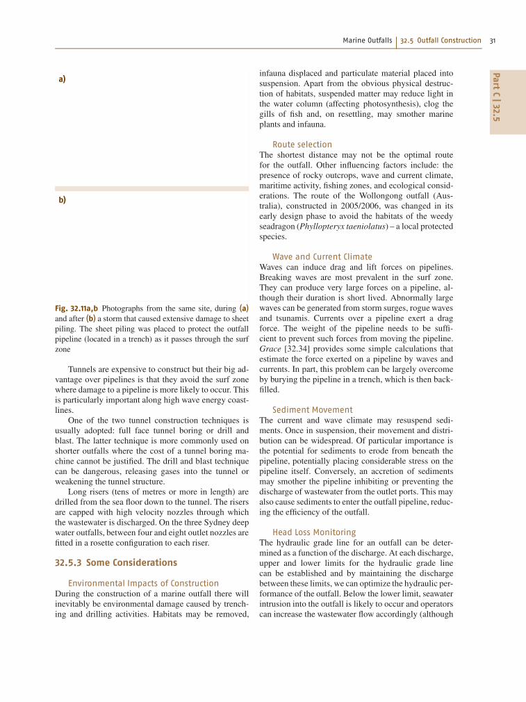
Marine Outfalls 32.5 Outfall Construction 31Part

C|32.5

a)

b)

Fig. 32.11a,b Photographs from the same site, during (a)and after (b) a storm that caused extensive damage to sheetpiling. The sheet piling was placed to protect the outfallpipeline (located in a trench) as it passes through the surfzone

Tunnels are expensive to construct but their big ad-vantage over pipelines is that they avoid the surf zonewhere damage to a pipeline is more likely to occur. Thisis particularly important along high wave energy coast-lines.

One of the two tunnel construction techniques isusually adopted: full face tunnel boring or drill andblast. The latter technique is more commonly used onshorter outfalls where the cost of a tunnel boring ma-chine cannot be justified. The drill and blast techniquecan be dangerous, releasing gases into the tunnel orweakening the tunnel structure.

Long risers (tens of metres or more in length) aredrilled from the sea floor down to the tunnel. The risersare capped with high velocity nozzles through whichthe wastewater is discharged. On the three Sydney deepwater outfalls, between four and eight outlet nozzles arefitted in a rosette configuration to each riser.

32.5.3 Some Considerations

Environmental Impacts of ConstructionDuring the construction of a marine outfall there willinevitably be environmental damage caused by trench-ing and drilling activities. Habitats may be removed,

infauna displaced and particulate material placed intosuspension. Apart from the obvious physical destruc-tion of habitats, suspended matter may reduce light inthe water column (affecting photosynthesis), clog thegills of fish and, on resettling, may smother marineplants and infauna.

Route selectionThe shortest distance may not be the optimal routefor the outfall. Other influencing factors include: thepresence of rocky outcrops, wave and current climate,maritime activity, fishing zones, and ecological consid-erations. The route of the Wollongong outfall (Aus-tralia), constructed in 2005/2006, was changed in itsearly design phase to avoid the habitats of the weedyseadragon (Phyllopteryx taeniolatus) – a local protectedspecies.

Wave and Current ClimateWaves can induce drag and lift forces on pipelines.Breaking waves are most prevalent in the surf zone.They can produce very large forces on a pipeline, al-though their duration is short lived. Abnormally largewaves can be generated from storm surges, rogue wavesand tsunamis. Currents over a pipeline exert a dragforce. The weight of the pipeline needs to be suffi-cient to prevent such forces from moving the pipeline.Grace [32.34] provides some simple calculations thatestimate the force exerted on a pipeline by waves andcurrents. In part, this problem can be largely overcomeby burying the pipeline in a trench, which is then back-filled.

Sediment MovementThe current and wave climate may resuspend sedi-ments. Once in suspension, their movement and distri-bution can be widespread. Of particular importance isthe potential for sediments to erode from beneath thepipeline, potentially placing considerable stress on thepipeline itself. Conversely, an accretion of sedimentsmay smother the pipeline inhibiting or preventing thedischarge of wastewater from the outlet ports. This mayalso cause sediments to enter the outfall pipeline, reduc-ing the efficiency of the outfall.

Head Loss MonitoringThe hydraulic grade line for an outfall can be deter-mined as a function of the discharge. At each discharge,upper and lower limits for the hydraulic grade linecan be established and by maintaining the dischargebetween these limits, we can optimize the hydraulic per-formance of the outfall. Below the lower limit, seawaterintrusion into the outfall is likely to occur and operatorscan increase the wastewater flow accordingly (although

PartC|32.6


increasing the flow may not always be possible). Theaddition of salinity sensors on individual risers can con-firm whether seawater intrusion has occurred.

Seawater Intrusion and PurgingA rule-of-thumb for preventing seawater from enter-ing the outfall is to keep the port densimetric Froudenumber (32.9) well above unity (e.g., on Sydney’sdeepwater ocean outfalls, the port densimetric Froudenumber is of the order of 20�30). Occasionally, the portdensimetric Froude number may become small and sea-water may enter the outfall. One method to help preventsuch an intrusion of seawater is to use nonreturn checkvalves. However, not all outfalls are so equipped andit may be necessary to periodically purge the seawaterfrom the outfall. This is done by backing up the wastew-ater in the treatment plant and releasing the wastewater

at high velocity. This also has the advantage of clearingthe outfall of sediments.

Outfall MaintenanceRegular inspections of the marine outfall should be car-ried out as part of a regular maintenance program toensure there is (a) no physical damage to any compo-nents and (b) no blockage of any outlet nozzles. Thiscan be carried out by divers although this is accom-panied by substantial health and safety concerns (e.g.,diving in contaminated waters, wave action, and decom-pression requirements for deep diving). Our preferenceis to carry out inspections using remotely operated ve-hicles. The frequency of maintenance inspections willdepend on a range of factors such as environmentalconditions and construction materials. Often, annual in-spections are adopted.

32.6 Environmental Monitoring

The fundamental objective of environmental monitor-ing is to quantify impacts that may arise as a result ofthe discharge of wastewater to the marine environment.Some of the questions that an environmental monitor-ing program should address include:

� Is it safe to swim?� Is it safe to eat the seafood?� Will the marine communities be protected into thefuture?� Will the beaches be free from contamination?

Two distinct environmental monitoring programsare often implemented. The first is a pre- and postcon-struction monitoring program. This is usually an intenseprogram of short duration (perhaps five years) aimedto quantify the initial impacts of the discharges fromthe marine outfall. The second is a long-term (ongo-ing) monitoring program, which usually takes a subsetof the information obtained from the pre- and post-construction monitoring program, and uses it to defineacceptable limits of change in the environmental indi-cators. Long-term monitoring is designed to determinewhether a subsequent change lies outside these limits.

There is an assumption, often tacit, that the en-gineering aspects of a sewage treatment system andmarine outfall are operating as designed. If there isa treatment bypass, breakdown or blockage of someof the outlet ports, the quality of the effluent (or itsdelivery to the marine environment) will be less thanexpected. Monitoring the operational performance is animportant element of environmental monitoring.

32.6.1 Change Versus Impact

The marine environment is in a state of continual flux.The challenge of a monitoring program is to separatechange that occurs via natural processes from changethat is a direct result of the discharge from the ma-rine outfall (i. e., impact). It is critical to define whatconstitutes an impact prior to the execution of the post-commissioning monitoring program. This places clearbounds on the interpretation of change that may be ob-served in the marine communities.

32.6.2 Pre- and PostconstructionMonitoring

Broadly, the pre- and postconstruction monitoring pro-gram compares conditions before and after the marineoutfall is commissioned. It is critical that sufficient timeis allowed to carry out the before monitoring. An aftermonitoring program can be conducted at any time af-ter commissioning of the marine outfall. However, weonly get one chance at the before phase of the monitor-ing program.

A monitoring program may be of several years’duration. Consequently, the cost of an environmentalmonitoring program may be large – perhaps 5% of theconstruction costs may be needed to properly addressthe main environmental issues.

Monitoring PhilosophySome of the characteristics that constitute a good mon-itoring program are outlined below. These characteris-

Marine Outfalls 32.6 Environmental Monitoring 33Part

C|32.6

tics combine to define our philosophy for environmentalmonitoring.

Environmental monitoring programs should be de-signed to establish cause-and-effect between the dis-charge and the environmental response. The approachwe favor uses weight-of-evidence. This simply meansapplying different techniques and approaches to thesame problem. If the answers that they provide areconsistent with what might be expected from such dis-charges, then we have greater confidence in the overallresult. Our weight-of-evidence is a three-pronged at-tack, which is detailed in the following section.

Most countries have guidelines (or licence condi-tions) that reflect the values that need to be protected.These values include social, public health and environ-mental aspects. While some values may be subjective,many can be quantified in terms of safe levels ofcontaminants that can be discharged. There is a tacitassumption, that by adhering to these concentration lim-its, there will be no irreversible damage done to themarine environment.

The most critical task in undertaking a monitoringprogram to quantify environmental impacts of a marineoutfall is to ask the right questions. This requires an un-derstanding of what is being discharged, what effectsthese discharges are likely to have on the marine en-vironment and the level of change that we are willingto accept. An answer to the wrong question, no matterhow accurate is that answer, will not allow impacts tobe quantified.

Environmental monitoring programs must be sci-entifically robust and defensible. We must test a hy-pothesis and gather empirical evidence to support (ordisprove) the hypothesis. The experiment must be re-peatable, cover a range of conditions and, in theory,repeated experiments should arrive at the same con-clusion. Marine outfalls may be contentious and themonitoring program may need to be defended. Oneway in which this can be done is via peer review ofthe work and publication of the results in a reputablejournal.

Conditions of approval for a marine outfall are oftenreliant on predictions. The objectives of an environmen-tal monitoring program should include the verification(or otherwise) of those predictions and whether theenvironmental values have been maintained. Further,the program should include a mechanism by whichproblems identified in the monitoring program can berectified or mitigated.

The Three-Pronged AttackAn approach to collecting weight-of-evidence for im-pact assessment includes three components. These aredetailed below.

Sources of Contaminants. There are many potentialsources of contaminants discharged to marine waters,including rivers, sediments (as both a source and sink),private and industrial outfalls, illegal dumping, andcoastal wastewater treatment plants. An important con-sideration to environmental monitoring is separating therelative contribution of an outfall from contributionsfrom the other sources. It may be possible to charac-terize (and isolate) the different sources via the types,concentrations, and variability of contaminants beingdischarged from each source.

Marine organisms may be impacted if exposed towastewater. Toxicity testing is a technique used to de-termine the concentration of substance which is likelyto harm to marine organisms. Whole effluent toxicity(WET) testing examines whether a toxic response isidentified when an organism is subjected to the com-plex wastewater matrix.

If toxicity testing is carried out using a single test or-ganism, it is then inferred that all marine organisms willexhibit the same toxic response. This is not necessar-ily the case and multiple organisms are recommendedfor toxicity testing: different organisms display differ-ent responses to different substances at different stagesin their life cycle. Ideally, a range of fish, inverte-brates, and algae at different stages in their life cycleshould be considered for toxicity testing. Toxicity testscan be either acute or chronic and both types of testsshould be included. The former determine the concen-tration of wastewater that is lethal to the test organism.Chronic testing examines the reduced capability (e.g.,impaired development or reproductive ability) of thetest organism.

Movement of Wastewater. Once we know what is be-ing discharged, we determine the path that the wastew-ater will take after discharge and how dilute it becomes.Emery and Thompson [32.36] describe many techniquesto measure and/or monitor the physical properties of themarine environment.

Instrumented moorings provide excellent temporalcoverage although the horizontal spatial coverage islimited by the number of such systems that the mon-itoring program can afford to deploy. Remote sensingprovides good spatial coverage of the region, althoughin general, the temporal scales are much longer thanthose associated with the movement of wastewaterplumes.

Numerical modeling enables us to predict how thewastewater will react to different marine conditions andto changes in the volume or method of discharge. It iscritical to calibrate and validate any numerical modelto ensure confidence in the results under existing con-ditions and for future scenarios. Coupled with this is

PartC|32.6


a need for confidence limits to be placed on modelresults. Too often model results are provided withouta real appreciation for the confidence that can be placedon those results.

Quantifying Change. There are a number of ap-proaches to quantifying change in response to a marineoutfall. One favored by the authors is the beyond BACIor mBACI approach [32.37]. BACI is an acronym forbefore, after, control, impact. Sites close to, and remotefrom, the outfall are monitored on several occasionsboth before and after commissioning of the marine out-fall. Perhaps the main reason that this is a favoredapproach is its emphasis on statistical power and sta-tistical error.

Statistical Errors. A Type I statistical error occurswhen the results of our analysis incorrectly predicts thata change has occurred. We can protect against makingsuch a mistake by specifying the level of significance.Usually this is set at 5% (equivalent to 95% confidencelimits), i. e., there is a 5% chance that our analysismakes a Type I statistical error.

A Type II statistical error occurs when the resultsof the analysis incorrectly predicts that a change hasnot occurred. From an environmental point of view, thisis more insidious than a Type I error because it incor-rectly leads us to believe that there is no environmentalproblem. It is difficult to protect against a Type II er-ror as this requires a priori knowledge of the variabilityin the system being measured. Such knowledge is ac-quired only after the monitoring is complete. Therefore,we need to use experience to estimate the system vari-ability and design experiments accordingly. To protectagainst making a Type II statistical error, we usually de-sign our experiments to target statistical power above80%. However, if statistical power is too high, verysmall changes become statistically significant and wequestion whether such small changes are meaningful. Itis critical to check the statistical power after the experi-ments have been completed.

Type III statistical errors occur when we arrive atthe correct answer but have asked the wrong question.

Some of the marine components measured to de-tect change as a result of a new marine outfall includewater quality, sediment quality and community studies(such as intertidal, plankton, pelagic, benthic, and ses-sile communities). Marine community studies shouldbe tailored for specific outfalls and might include:

� Intertidal community studies for shoreline or shortoutfalls.� Subtidal settlement panel studies for marine outfallin waters less than about 20 m depth (much deeper

than this and the light attenuation starts to inhibitthe growth of organisms on the settlement panels).� Fish, shellfish, and planktonic communities movein, and with, marine waters. The variability amongcontrol sites may be as much as the variability be-tween putatively impacted sites and control sites.Therefore, it may be difficult to isolate the marineoutfall as the cause of change in such communities.� Sediments have been used to assess the accumu-lation of contaminants and to examine infaunacommunity variations. Our experience is that suchstudies have limited success. Unless the contami-nant signal is very strong, it is unlikely to register ina sediment sample.� Bioaccumulation studies are sometimes recom-mended as impact assessment indicators. However,caution is needed when interpreting the results ofsuch studies because:– Fish move, and it is not always possible to know

the region from where contaminants were ac-cumulated. This necessitates fish home rangestudies, which can be expensive and, perhaps,inconclusive.

– Species that are caught at one particular timeand location may not be caught at other timesor locations and pooling into higher biologi-cal levels may be required. Different speciesmay accumulate different substances at differentrates and the pooling process may mask poten-tial impacts.

– Moored systems comprising oysters or musselsare often used in bioaccumulation studies. How-ever, this may involve removing the animalsfrom their natural habitat thereby, adding stressto the organisms and confounding the resultsthat are obtained.

32.6.3 Long-Term Monitoring

The pre- and postconstruction monitoring program willidentify whether there has been a step change in thebaseline conditions as a result of the discharge fromthe marine outfall. Long-term monitoring is used toidentify whether further change occurs well after themarine outfall has been commissioned. It can be usedto extrapolate trends and, where necessary, design andimplement an appropriate mitigation strategy to pre-vent, or reverse, the trend. The three-pronged attackdescribed in Sect. 32.6.2 is also applicable to long-termmonitoring.

However, there is a temptation to simply implementthe bulk of the pre- and postconstruction monitoringprogram as part of the long-term monitoring program.Apart from the expense associated in maintaining a de-

Marine Outfalls References 35Part

C|32.6

tailed monitoring program over a long period of time,environmental changes will be masked by the smalltime steps between consecutive sets of readings. It maybe more effective to implement a low level, long-termmonitoring program and revisit the detailed monitoringprogram, for example, over two consecutive years ev-ery 10 yr. If the long-term program indicates a potentialproblem, it provides the motivation for a more detailedinvestigation.

Where such an approach is adopted, source charac-terization combined with numerical modeling are usedto estimate environmental impact. If the results indicatea possible impact, confirmation studies can be imple-mented.

32.6.4 Summary

This chapter provides a synopsis of the discharge ofwastewater to the marine environment. Flows of ef-fluent from municipal sewage treatment plants andbrine from desalination plants are primarily consideredwithin the context of near-field modeling and outfall hy-draulics. The designers of outfalls are under increasingpressure from social, public health and environmentalconstraints, within a regulatory and economic frame-work, all of which need to be considered. This compactoverview exposes the reader to fundamentals of outfalldesign and identifies some of the traps and problemsthat may arise.

References

32.1 P.M. Tate, J.H. Middleton: Buoyant jets of ellipticshape: Approximation for duckbill valves, J. Hy-draul. Eng. 130(5), 432–440 (2004)

32.2 Metcalf & Eddy Inc., G. Tchobanoglous, F.L. Burton,H.D. Stensel: Wastewater Engineering: Treatmentand Reuse, 4th edn. (McGraw-Hill, New York 2003)

32.3 P. Palomar, I.J. Losada: Impacts of brine dischargeon the marine environment. Modelling as a pre-dictive tool. In: Desalination, Trends and Tech-nologies, ed. by M. Schorr (InTech, Rijeka 2010)pp. 279–310

32.4 I.R. Wood, R.G. Bell, D.L. Wilkinson: Ocean Disposalof Waste (World Scientific, Singapore 1993)

32.5 J.H. Lee, V. Cheung: Generalized Lagrangian modelfor buoyant jets in current, J. Environ. Eng. 116(6),1085–1106 (1990)

32.6 P.M. Tate, J.H. Middleton: Unification of non-dimensional solutions to asymptotic equations forplumes of different shape, Boundary-Layer Mete-orol. 94(2), 225–251 (2000)

32.7 G.H. Jirka, P.J. Akar: Hydrodynamic classificationof submerged multiport-diffuser discharges, J. Hy-draul. Eng. 117(9), 1113–1128 (1991)

32.8 G.H. Jirka, R.L. Domeker: Hydrodynamic classifica-tion of submerged single-port discharges, J. Hy-draul. Eng. 117(9), 1095–1112 (1991)

32.9 B. Morton, G. Taylor, J. Turner: Turbulent gravi-tational convection from maintained and instan-taneous sources, Proc. R. Soc. A 234(1196), 1–23(1956)

32.10 L.-N. Fan: Turbulent Buoyant Jets into Stratified orFlowing Ambient Fluids, Technical Report (CALTECH,Pasadena 1967)

32.11 C.C. Lai, J.H. Lee: Mixing of inclined dense jets instationary ambient, J. Hydroenviron. Res. 6(1), 9–28 (2012)

32.12 P.J. Roberts, A. Ferrier, G. Daviero: Mixing in in-clined dense jets, J. Hydraul. Eng. 123(7), 693–699(1997)

32.13 A. Cipollina, A. Brucato, F. Grisafi, S. Nicosia:Bench-scale investigation of inclined dense jets,J. Hydraul. Eng. 131(11), 1017–1022 (2005)

32.14 S. Nemlioglu, P. Roberts: Experiments on densejets using three-dimensional laser-induced fluo-rescence (3DLIF), Proc. 4th Int. Conf. MWWD, Antalya(2006)

32.15 G. Kikkert, M. Davidson, R. Nokes: Inclined nega-tively buoyant discharges, J. Hydraul. Eng. 133(4),545–554 (2007)

32.16 D. Shao, A.W.-K. Law: Mixing and boundary inter-actions of 30 and 45 inclined dense jets, Environ.Fluid Mech. 10(5), 521–553 (2010)

32.17 I.G. Papakonstantis, G.C. Christodoulou, P.N. Pa-panicolaou: Inclined negatively buoyant jets 1: Ge-ometrical characteristics, J. Hydraul. Res. 49(1), 3–12(2011)

32.18 I.G. Papakonstantis, G.C. Christodoulou, P.N. Pa-panicolaou: Inclined negatively buoyant jets 2:Concentration measurements, J. Hydraul. Res.49(1), 13–22 (2011)

32.19 V.H. Chu: L.N. Fan’s data on buoyant jets in cross-flow, J. Hydraul. Div. 105(4), 612–617 (1979)

32.20 P.J. Roberts, H.J. Salas, F.M. Reiff, M. Libhaber: Ma-rine Wastewater Outfalls and Treatment Systems(IWA Publishing, London 2010)

32.21 B. Henderson-Sellers: Modeling of Plume Rise andDispersion-The University of Salford Model: USPR,Lecture Notes in Engineering, Vol. 25 (Springer,Berlin Heidelberg 1987)

32.22 H.B. Fischer, E.J. List, R.C.Y. Koh, J. Imberger,N.H. Brooks: Mixing in Inland and Coastal Waters(Academic, New York 1979)

32.23 D.L. Wilkinson: Optimal design of ocean outfalls. In:Environmental Hydraulics, ed. by C.C. Lai, J.H. Lee(Balkema, Rotterdam 1991) pp. 275–279

32.24 S.I. Seneviratne, N. Nicholls, D. Easterling,C.M. Goodess, S. Kanae, J. Kossin, Y. Luo,J. Marengo, K. McInnes, M. Rahimi, M. Reich-stein, A. Sorteberg, C. Vera, X. Zhang: Changes inclimate extremes and their impacts on the naturalphysical environment. In: Managing the Risks ofExtreme Events and Disasters to Advance ClimateChange Adaptation, ed. by C.B. Field, V. Barros,T.F. Stocker, D. Qin, D.J. Dokken, K.L. Ebi, M.D. Mas-

PartC|32.6


trandrea, K.J. Mach, G.-K. Plattner, S.K. Allen,M. Tignor, P.M. Midgley (Cambridge Univ. Press,Cambridge 2012) pp. 109–230

32.25 M.H. Sharqawy, J.H. Lienhard, S.M. Zubair: Ther-mophysical properties of seawater: A review ofexisting correlations and data, Desalin. Water Treat.16(1-3), 354–380 (2010)

32.26 J. Pitt, P. Ackers: Hydraulic Roughness of Segmen-tally Lined Tunnels (CIRIA, London 1982)

32.27 D.S. Miller: Internal Flow Systems (Miller Innova-tions, Bedford 2009)

32.28 I. Idelchik: Handbook of Hydraulic Resistance(Jaico, Mumbai 2003)

32.29 D.L. Wilkinson: Avoidance of seawater intrusioninto ports of ocean outfalls, J. Hydraul. Eng. 114(2),218–228 (1988)

32.30 W.H. Hager: Wastewater Hydraulics: Theory andPractice (Springer, Berlin Heidelberg 2010)

32.31 H.T. Falvey: Air-Water Flow in Hydraulic Structures,Technical Report (Water and Power Resources Ser-vice, Denver 1980)

32.32 C.S. Lauchlan, R.W.P. May, R. Burrows, C. Gahan: Airin Pipelines: A Literature Review (HR Ltd., Walling-ford 2005)

32.33 D. Butler, R.W.P. May, J.C. Ackers: Sediment trans-port in sewers part 1: Background, Proc. ICE-WaterMarit. Energy, Vol. 118 (1996) pp. 103–112

32.34 R.A. Grace: Marine Outfall Systems. Planning, De-sign and Construction (Prentice-Hall, Upper SaddleRiver 1978)

32.35 R.A. Grace: Marine Outfall Construction: Back-ground, Techniques, and Case Studies (ASCE, Reston2009)

32.36 W.J. Emery, R.E. Thomson: Data Analysis Methodsin Physical Oceanography (Pergamon, Oxford 1998)

32.37 A. Underwood: Beyond BACI: Experimental designsfor detecting human environmental impacts ontemporal variations in natural populations, Mar.Freshw. Res. 42(4), 569–587 (1991)

32.38 32nocite]Please cite this reference in the text. Oth-erwise it must be deleted.M.S. Field, R.G. Wilhelm,J.F. Quinlan, T.J. Aley: An assessment of the po-tential adverse properties of fluorescent tracer dyesused for groundwater tracing, Environ. Monit. As-sess. 38(1), 75–96 (1995)

32.39 C. Leibundgut, S. Hadi: A contribution to toxicity offluorescent tracers. In: Tracer Hydrology, Vol. 97, ed.by A. Kranjc (Balkema, Rotterdam 1997)

http://www.springer.com/978-3-319-16648-3

32. marine outfalls

Documents