3.2 Using a Relational Database from Java

(Sciore, 2008, Chapter 8)

• We shall consider the SimpleDB server side structure later in this course.

• Let us consider here the structure for a simple client.

• There is a family of client-server database communication protocols called OpenData Base Connectivity (ODBC).

• There are now ODBC binding libraries for many programming languages. Theypermit application programs written in that language to communicate with anyODBC-compliant database server.

• The Java binding is called JDBC – which does not mean “Java DBC” according toSun’s legal position. . .

• The SimpleDB supports enough of the JDBC specification to allow writing simpleclients – but not nearly all the features of the whole specification.

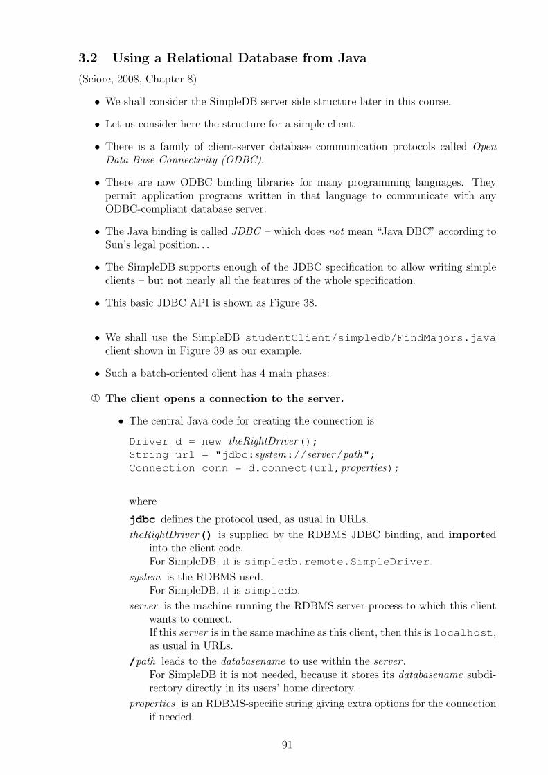
• This basic JDBC API is shown as Figure 38.

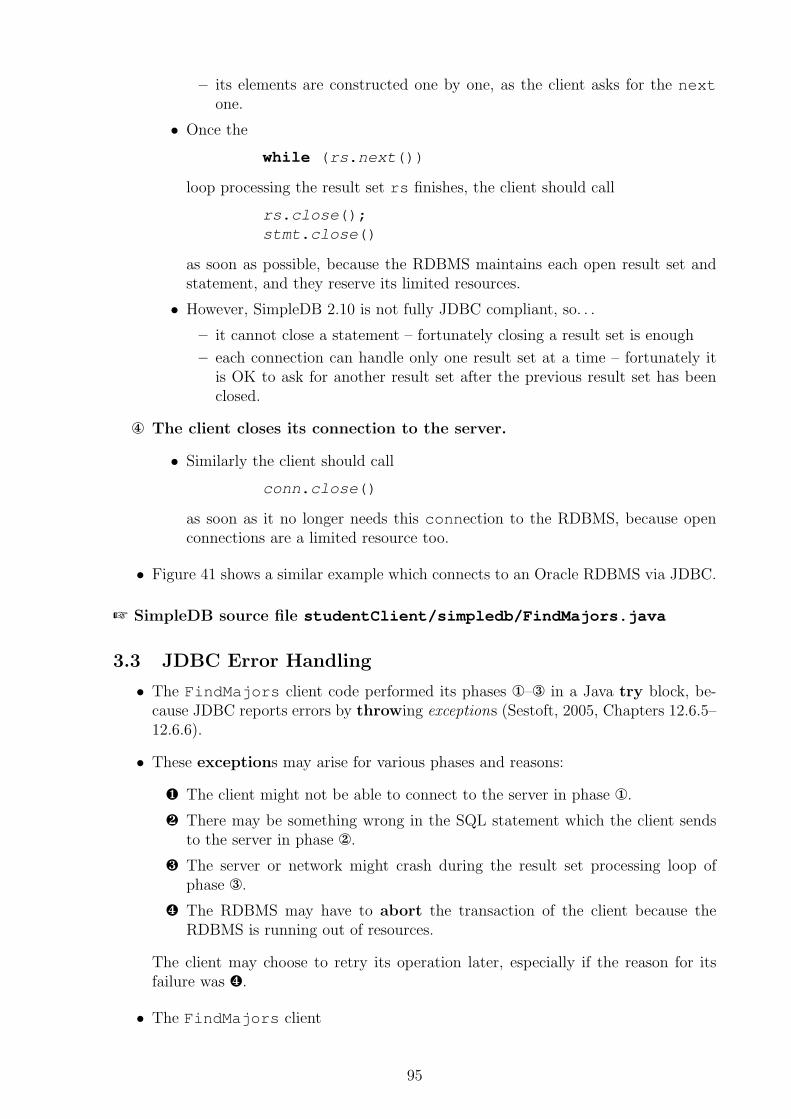
• We shall use the SimpleDB studentClient/simpledb/FindMajors.java

client shown in Figure 39 as our example.

• Such a batch-oriented client has 4 main phases:

¬ The client opens a connection to the server.

• The central Java code for creating the connection is

Driver d = new theRightDriver();String url = "jdbc:system://server/path";Connection conn = d.connect(url,properties);

where

jdbc defines the protocol used, as usual in URLs.

theRightDriver() is supplied by the RDBMS JDBC binding, and importedinto the client code.For SimpleDB, it is simpledb.remote.SimpleDriver.

system is the RDBMS used.For SimpleDB, it is simpledb.

server is the machine running the RDBMS server process to which this clientwants to connect.If this server is in the same machine as this client, then this is localhost,as usual in URLs.

/path leads to the databasename to use within the server .For SimpleDB it is not needed, because it stores its databasename subdi-rectory directly in its users’ home directory.

properties is an RDBMS-specific string giving extra options for the connectionif needed.

91

Figure 38: The basic JDBC Application Programming Interface. (Sciore, 2008)

92

– For instance, if the RDBMS has mandatory access control, then thisstring can contain the required username and password.

– SimpleDB does not support any properties so it is the null pointer.

• The vendor-independent parts of JDBC are imported from java.sql.*.

• The method calls of this created connection go to the Remote Method Invo-cation (RMI) registry running on the server .

– This is the rmiregistry mentioned in Section 3.1.

– It is the “phone directory” for Java methods which can be called fromother processes, even across the network.

– When the SimpleDB server starts, it registers its public methods there,so that its client processes can invoke them to ask the server to performdatabase operations.

• Unfortunately this old way to form the connection is not very portable, be-cause the client must contain theRightDriver which is vendor-dependent.

• Java supports also new ways, where the server can send theRightDriver to itsclients based on the system in the url (Sciore, 2008, Chapter 8.2.1).

+ Now the client is vendor-independent, but. . .

− the server-side setup gets more complicated, and so we continue using theold way here instead.

­ The client sends an SQL statement to the server.

• The central Java code for querying the database is

Statement stmt = conn.createStatement();

String qry = statement;ResultSet rs = stmt.executeQuery(qry);

where

statement is an SQL SELECT. . .FROM. . .WHERE. . . statement as text.

rs gives the results of the query as a result set to be processed in the nextphase ®.

• Other SQL statements can be issued with

int howMany = stmt.executeUpdate(qry);

whose return value tells how many records were affected instead of a result set.

• The RDBMS server

¶ first compiles this statement into Relational Algebra and optimizes it intoa form. . .

· which it then executes.

• A statement can also be prepared beforehand:

– The compilation step ¶ happens only once.

– The same compiled statement can be executed in step · many times withdifferent parameter values each time.

93

• These prepared statements are

efficient because we shall see during this course that the compilation step ¶

is not trivial

safer because their vendor-supplied implementation is probably more robustthan our own handwritten code.For instance, handwritten code may be vulnerable to the SQL injectionattack which permits the attacker to execute arbitrary SQL commandsagainst our database. . .

• These parameter positions are marked with question marks ‘?’ within thestatement to prepare, while the value for the nth ‘?’ can be set with themethod

setType(int n,Type value)

for each SQL Type.

• Figure 40 shows an example, where the same parameterized query is used in aloop to query the students of different majors.

® The client receives the result from the server.

• The result set of a query consists of the corresponding rows. One of them isthe current row – a reading position within the result set.

– Initially this current row is just before the first row of the result set – soit is not valid yet.

– Method next moves this current row to the next row of the result set. Itreturns false if it moved past the last row of the result set – so it is nolonger valid.

– If the current row is valid, then the value for its named attribute can beextracted with the method

Type getType(String name)

for each SQL Type.

– Note: Figure 38 did not mention this name parameter.

• SimpleDB uses this current row model also for its internal intermediate resultsets of individual Relational Algebra operators.

• This current row model is the same as in the iterators for Java collections (Ses-toft, 2005, Chapters 22.1, 22.7 and 12.5.2) discussed in the course “Data Struc-tures and Algorithms I” (“Tietorakenteet ja algoritmit I” (TRAI) in Finnish).

• Besides these basic “read forward” result sets, JDBC also supports

scrollable result sets, whose current row can move also backwards, and

updatable result sets, which permit updating the attribute values of thecurrent row

(Sciore, 2008, Chapter 8.2.5) which are especially useful in clients with graph-ical user interfaces (GUIs).

• Such a result set is an example of a lazy data structure:

– it does not exist as a whole, but. . .

94

– its elements are constructed one by one, as the client asks for the nextone.

• Once the

while (rs.next())

loop processing the result set rs finishes, the client should call

rs.close();

stmt.close()

as soon as possible, because the RDBMS maintains each open result set andstatement, and they reserve its limited resources.

• However, SimpleDB 2.10 is not fully JDBC compliant, so. . .

– it cannot close a statement – fortunately closing a result set is enough

– each connection can handle only one result set at a time – fortunately itis OK to ask for another result set after the previous result set has beenclosed.

¯ The client closes its connection to the server.

• Similarly the client should call

conn.close()

as soon as it no longer needs this connection to the RDBMS, because openconnections are a limited resource too.

• Figure 41 shows a similar example which connects to an Oracle RDBMS via JDBC.

+ SimpleDB source file studentClient/simpledb/FindMajors.java

3.3 JDBC Error Handling

• The FindMajors client code performed its phases ¬–® in a Java try block, be-cause JDBC reports errors by throwing exceptions (Sestoft, 2005, Chapters 12.6.5–12.6.6).

• These exceptions may arise for various phases and reasons:

¶ The client might not be able to connect to the server in phase ¬.

· There may be something wrong in the SQL statement which the client sendsto the server in phase ­.

¸ The server or network might crash during the result set processing loop ofphase ®.

¹ The RDBMS may have to abort the transaction of the client because theRDBMS is running out of resources.

The client may choose to retry its operation later, especially if the reason for itsfailure was ¹.

• The FindMajors client

95

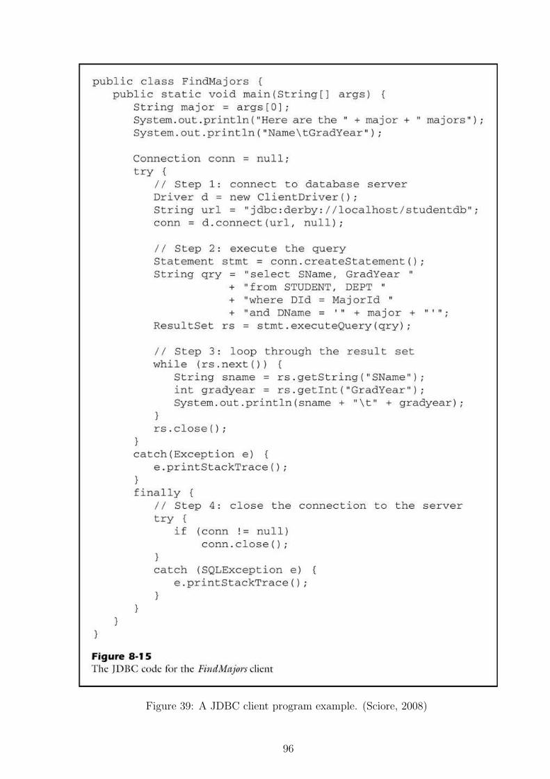
Figure 39: A JDBC client program example. (Sciore, 2008)

96

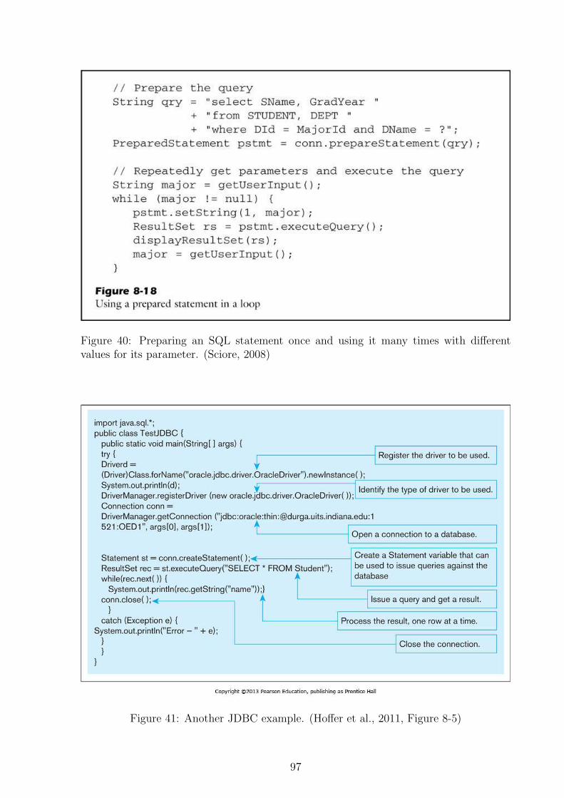
Figure 40: Preparing an SQL statement once and using it many times with differentvalues for its parameter. (Sciore, 2008)

Figure 41: Another JDBC example. (Hoffer et al., 2011, Figure 8-5)

97

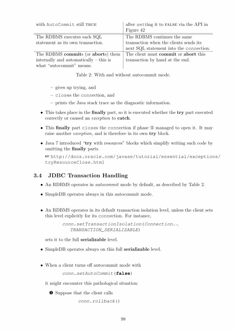
with AutoCommit still true after setting it to false via the API inFigure 42

The RDBMS executes each SQLstatement as its own transaction.

The RDBMS continues the sametransaction when the clients sends itsnext SQL statement into the connection.

The RDBMS commits (or aborts) theminternally and automatically – this iswhat “autocommit” means.

The client must commit or abort thistransaction by hand at the end.

Table 2: With and without autocommit mode.

– gives up trying, and

– closes the connection, and

– prints the Java stack trace as the diagnostic information.

• This takes place in the finally part, so it is executed whether the try part executedcorrectly or caused an exception to catch.

• This finally part closes the connection if phase ¬ managed to open it. It mayraise another exception, and is therefore in its own try block.

• Java 7 introduced “try with resources” blocks which simplify writing such code byomitting the finally parts.

+ http://docs.oracle.com/javase/tutorial/essential/exceptions/

tryResourceClose.html

3.4 JDBC Transaction Handling

• An RDBMS operates in autocommit mode by default, as described by Table 2.

• SimpleDB operates always in this autocommit mode.

• An RDBMS operates in its default transaction isolation level, unless the client setsthis level explicitly for its connection. For instance,

conn.setTransactionIsolation(Connection.ց

TRANSACTION_SERIALIZABLE)

sets it to the full serializable level.

• SimpleDB operates always on this full serializable level.

• When a client turns off autocommit mode with

conn.setAutoCommit(false)

it might encounter this pathological situation:

¶ Suppose that the client calls

conn.rollback()

98

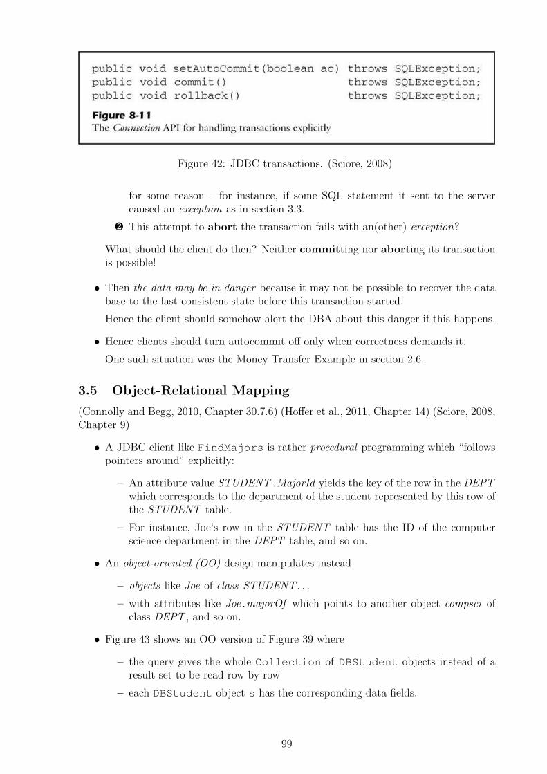
Figure 42: JDBC transactions. (Sciore, 2008)

for some reason – for instance, if some SQL statement it sent to the servercaused an exception as in section 3.3.

· This attempt to abort the transaction fails with an(other) exception?

What should the client do then? Neither committing nor aborting its transactionis possible!

• Then the data may be in danger because it may not be possible to recover the database to the last consistent state before this transaction started.

Hence the client should somehow alert the DBA about this danger if this happens.

• Hence clients should turn autocommit off only when correctness demands it.

One such situation was the Money Transfer Example in section 2.6.

3.5 Object-Relational Mapping

(Connolly and Begg, 2010, Chapter 30.7.6) (Hoffer et al., 2011, Chapter 14) (Sciore, 2008,Chapter 9)

• A JDBC client like FindMajors is rather procedural programming which “followspointers around” explicitly:

– An attribute value STUDENT .MajorId yields the key of the row in the DEPTwhich corresponds to the department of the student represented by this row ofthe STUDENT table.

– For instance, Joe’s row in the STUDENT table has the ID of the computerscience department in the DEPT table, and so on.

• An object-oriented (OO) design manipulates instead

– objects like Joe of class STUDENT . . .

– with attributes like Joe .majorOf which points to another object compsci ofclass DEPT , and so on.

• Figure 43 shows an OO version of Figure 39 where

– the query gives the whole Collection of DBStudent objects instead of aresult set to be read row by row

– each DBStudent object s has the corresponding data fields.

99

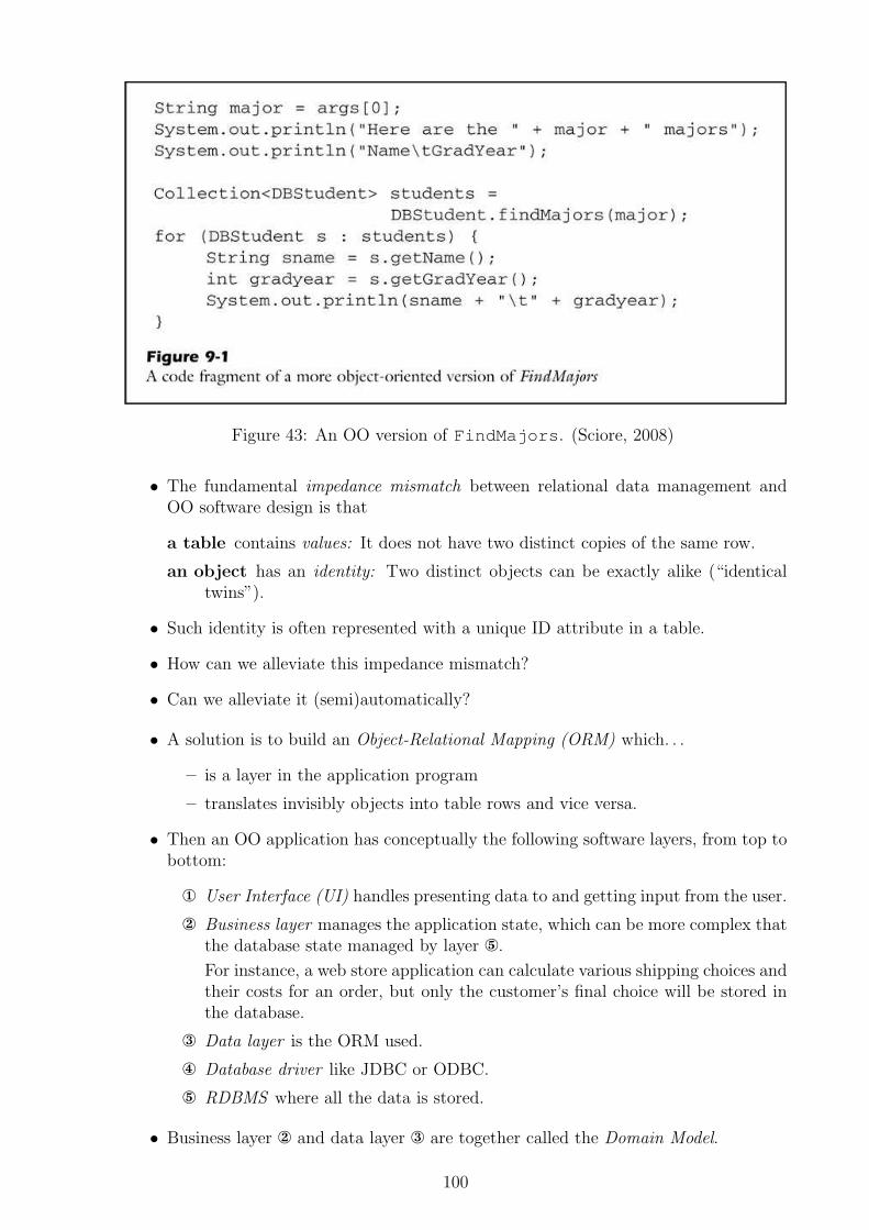
Figure 43: An OO version of FindMajors. (Sciore, 2008)

• The fundamental impedance mismatch between relational data management andOO software design is that

a table contains values: It does not have two distinct copies of the same row.

an object has an identity: Two distinct objects can be exactly alike (“identicaltwins”).

• Such identity is often represented with a unique ID attribute in a table.

• How can we alleviate this impedance mismatch?

• Can we alleviate it (semi)automatically?

• A solution is to build an Object-Relational Mapping (ORM) which. . .

– is a layer in the application program

– translates invisibly objects into table rows and vice versa.

• Then an OO application has conceptually the following software layers, from top tobottom:

¬ User Interface (UI) handles presenting data to and getting input from the user.

­ Business layer manages the application state, which can be more complex thatthe database state managed by layer °.

For instance, a web store application can calculate various shipping choices andtheir costs for an order, but only the customer’s final choice will be stored inthe database.

® Data layer is the ORM used.

¯ Database driver like JDBC or ODBC.

° RDBMS where all the data is stored.

• Business layer ­ and data layer ® are together called the Domain Model.

100

– This “domain” means “what this application is designed for”, like “placingorders in a web store”.

– Its layer ­ tells how the different objects of this application domain interactwith each other.

– Its layer ® tells which of these objects are persistent – saved between differentexecutions of the application.

– Unfortunately also relational database theory uses these same words “domain”and “model”, but they mean entirely different concepts there. . .

• The Java Persistence Architecture (JPA) is one tool for generating an ORM ® ontop of JDBC ¯.

• JPA attempts to be the standard for Java persistent objects, which have been offeredin various incompatible ways before.

• OpenJPA + http://openjpa.apache.org/ is one free JPA implementation.

• JPA uses Java code tagged with the relational table design, as in Figure 44.

– Consider the class diagram for our University example in Figure 3 (or theExtended Entity-Relationship (EER) diagram (Hoffer et al., 2011, Chapters 2–4) (Connolly and Begg, 2010, Chapters 12 and 13) if that was used instead).

– We assume for simplicity that set-valued attributes have already been turnedinto relationships in this diagram, so it is “in 1NF” (although strictly speakingsuch design diagrams do not have normal forms).

– Each class (or entity) in the diagram corresponds to a class in the Java program.

∗ Such a Java class is tagged with @Entity.

∗ Another tag @Table{name=X} tells the database table X where theseentities are stored.

∗ In Figure 44, we are tagging that the table STUDENT stores the objects ofentity class Student which represents a student.

– Each field in the class (or entity) becomes a field of the object, tagged with@Column{name=Y} telling the table attribute X.Y where its contents arestored.

– The primary key of table X is also added as such a field, and tagged with @Id

to say that it provides the object identity.

– Each relationship (or “line”) A—B between classes (or entities) A and B in thediagram is represented as two fields.

∗ Each endpoint corresponds to a Java class. This Java class gets one field.This field represents this relationship seen from this endpoint towards theother endpoint.

∗ This field for A formed by looking from A towards B (and vice versa forthe other field).

∗ If we look from STUDENT towards his/her majoring DEPT in Figure 3,we see a many-to-one (“m : 1”) relationship.

∗ But if we look from STUDENT towards his/her course ENROLLments,we see a one-to-many (“1 : m”) relationship.

101

– If the other endpoint B has ”1” then the field at this endpoint A will be likethis:

∗ It will have the type “one reference to an object of class B” – in Java: B.

∗ Thus we have the field Student.major of type Dept.

∗ It is tagged with @ManyToOne to express this cardinality.

∗ The table at this endpoint must also have a foreign key F referencing theother endpoint. It is given as the tag @JoinColumn{name=F}.

∗ Thus we have F = MajorId by Figure 6.

∗ If the other endpoint has cardinality 0..1 (“at most one”) then this field ispermitted to be NULL.

– If the other endpoint B has ”m” then the field at this endpoint A will be likethis instead:

∗ It will have the type “many references to objects of class B” where B

corresponds to the other endpoint – in Java: Collection<B>.

∗ Thus field Student.enrollments has type Collection<Enroll>.

∗ The class of the other endpoint must have some field B.G which representsthis relation in the other direction B—A.

∗ This field is tagged with @OneToMany{mappedBy=G} to express thiscardinality and the other direction.

∗ Thus we assume G = student.

• Now we can use JPA to access the data as objects in Figure 46:

¬ First we create a javax.jpa.EntityManager for our database.

– It keeps track of persistent objects – like the Connection kept track ofStatements and their ResultSets in JDBC.

– Its two-step creation provides flexibility: this same initialization codeworks both for stand-alone applications and web services.

­ We must start our own transaction, because want to make either all our changesin parts ¯ and ° to the persistent objects or none of them.

® We use our EntityManager to find the object of class Dept whose @Idfield is 20 – the object for the Mathematics Department.

– The EntityManager ensures that we do not have two different “live”copies in RAM of the same persistent object.

– It does this by checking if it has already constructed such an object before.In other words, it maintains a cache of persistent objects internally.

– Two different EntityManagers (maybe running on two different com-puters) do have their own “live” copies of the same persistent object.It is the job of the database transaction management to coordinate changesinto the database when each EntityManager tries to commit its changesas in part ±.

¯ We add a new Mathematics student s and make him persistent.

By default, JPA creates only “vanilla” Java transient objects which disappearwhen the application quits.

° We change his graduation year into 2011 and delete all his Enrollments.

102

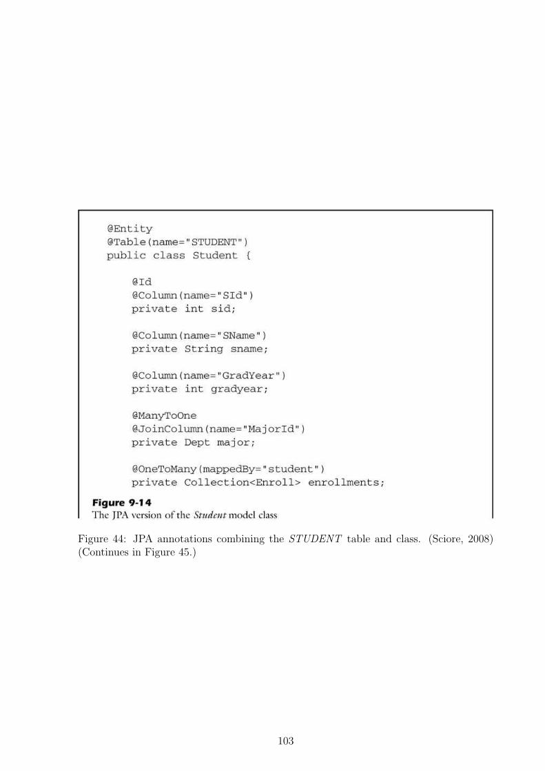
Figure 44: JPA annotations combining the STUDENT table and class. (Sciore, 2008)(Continues in Figure 45.)

103

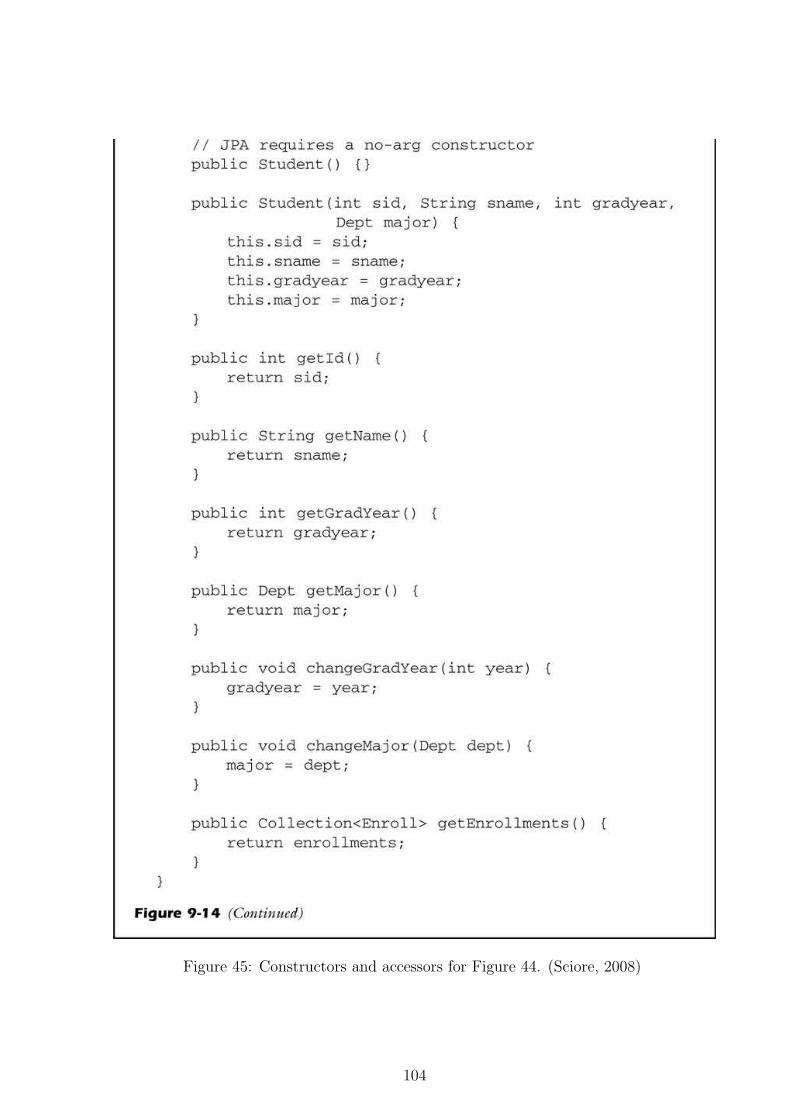
Figure 45: Constructors and accessors for Figure 44. (Sciore, 2008)

104

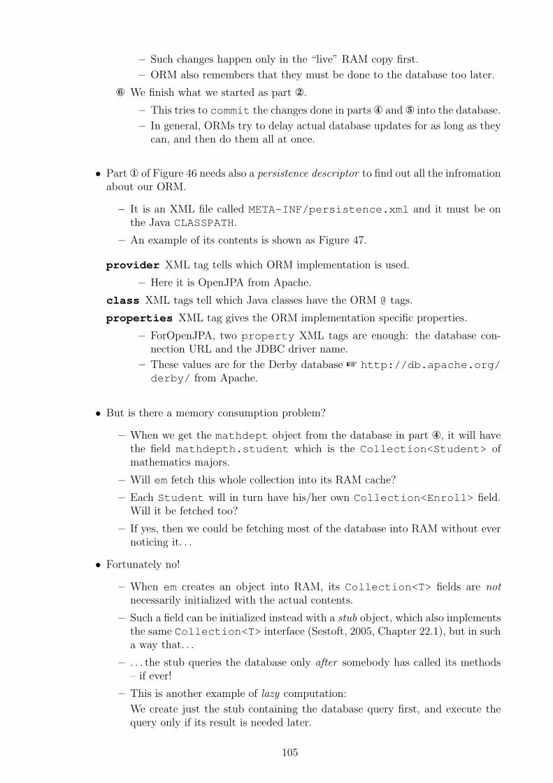
– Such changes happen only in the “live” RAM copy first.

– ORM also remembers that they must be done to the database too later.

± We finish what we started as part ­.

– This tries to commit the changes done in parts ¯ and ° into the database.

– In general, ORMs try to delay actual database updates for as long as theycan, and then do them all at once.

• Part ¬ of Figure 46 needs also a persistence descriptor to find out all the infromationabout our ORM.

– It is an XML file called META-INF/persistence.xml and it must be onthe Java CLASSPATH.

– An example of its contents is shown as Figure 47.

provider XML tag tells which ORM implementation is used.

– Here it is OpenJPA from Apache.

class XML tags tell which Java classes have the ORM @ tags.

properties XML tag gives the ORM implementation specific properties.

– ForOpenJPA, two property XML tags are enough: the database con-nection URL and the JDBC driver name.

– These values are for the Derby database + http://db.apache.org/

derby/ from Apache.

• But is there a memory consumption problem?

– When we get the mathdept object from the database in part ¯, it will havethe field mathdepth.student which is the Collection<Student> ofmathematics majors.

– Will em fetch this whole collection into its RAM cache?

– Each Student will in turn have his/her own Collection<Enroll> field.Will it be fetched too?

– If yes, then we could be fetching most of the database into RAM without evernoticing it. . .

• Fortunately no!

– When em creates an object into RAM, its Collection<T> fields are notnecessarily initialized with the actual contents.

– Such a field can be initialized instead with a stub object, which also implementsthe same Collection<T> interface (Sestoft, 2005, Chapter 22.1), but in sucha way that. . .

– . . . the stub queries the database only after somebody has called its methods– if ever!

– This is another example of lazy computation:

We create just the stub containing the database query first, and execute thequery only if its result is needed later.

105

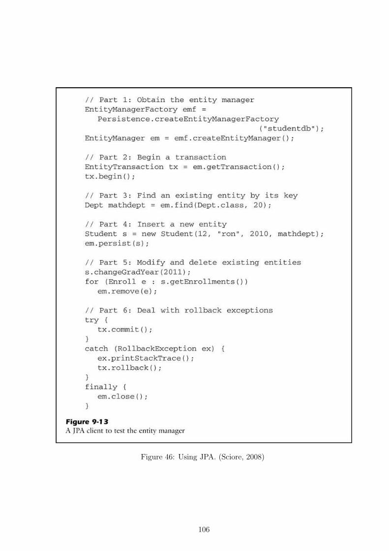
Figure 46: Using JPA. (Sciore, 2008)

106

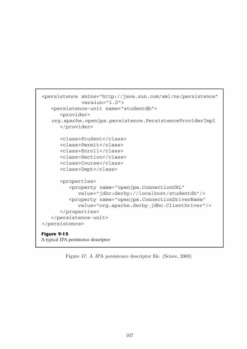
Figure 47: A JPA persistence descriptor file. (Sciore, 2008)

107

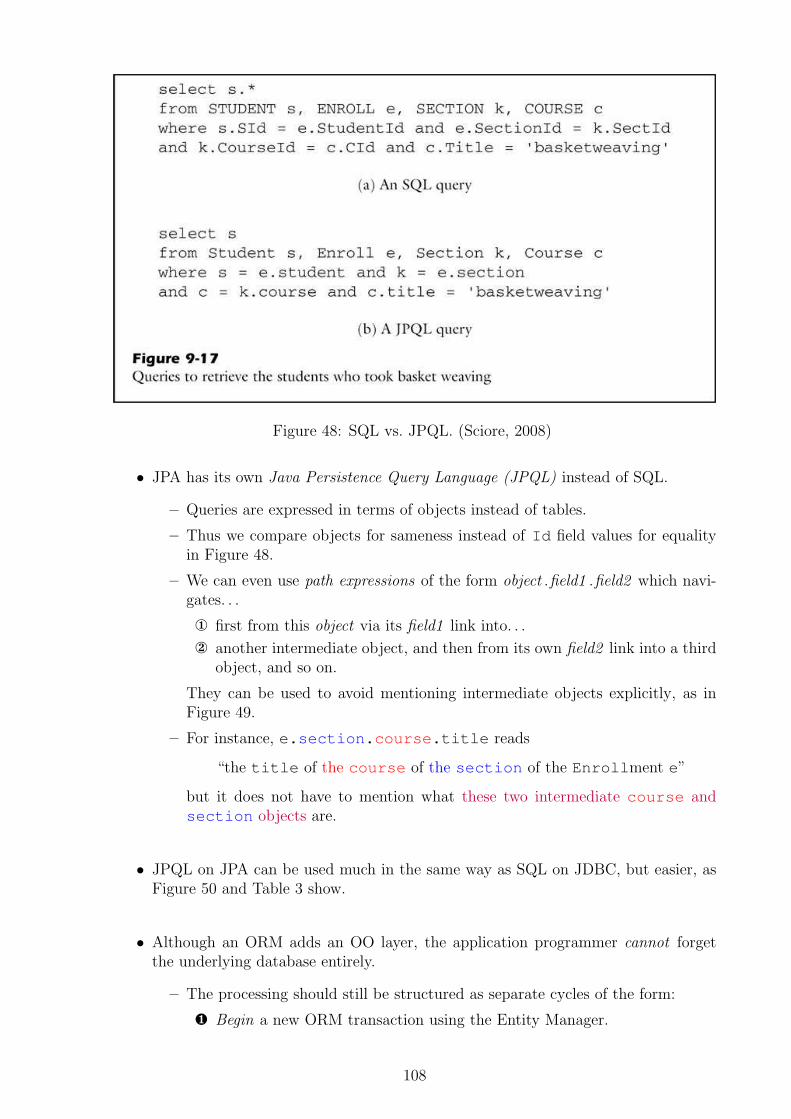
Figure 48: SQL vs. JPQL. (Sciore, 2008)

• JPA has its own Java Persistence Query Language (JPQL) instead of SQL.

– Queries are expressed in terms of objects instead of tables.

– Thus we compare objects for sameness instead of Id field values for equalityin Figure 48.

– We can even use path expressions of the form object .field1 .field2 which navi-gates. . .

¬ first from this object via its field1 link into. . .

­ another intermediate object, and then from its own field2 link into a thirdobject, and so on.

They can be used to avoid mentioning intermediate objects explicitly, as inFigure 49.

– For instance, e.section.course.title reads

“the title of the course of the section of the Enrollment e”

but it does not have to mention what these two intermediate course andsection objects are.

• JPQL on JPA can be used much in the same way as SQL on JDBC, but easier, asFigure 50 and Table 3 show.

• Although an ORM adds an OO layer, the application programmer cannot forgetthe underlying database entirely.

– The processing should still be structured as separate cycles of the form:

¶ Begin a new ORM transaction using the Entity Manager.

108

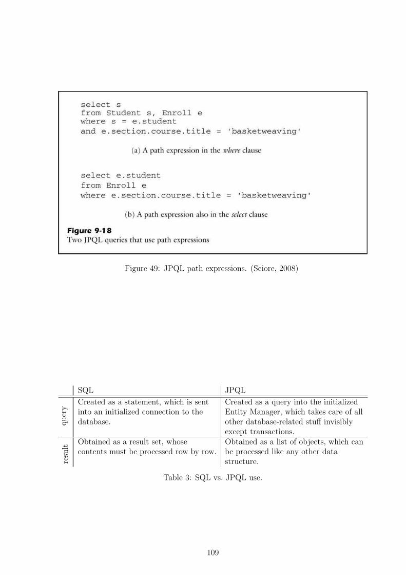
Figure 49: JPQL path expressions. (Sciore, 2008)

SQL JPQL

quer

y

Created as a statement, which is sentinto an initialized connection to thedatabase.

Created as a query into the initializedEntity Manager, which takes care of allother database-related stuff invisiblyexcept transactions.

resu

lt

Obtained as a result set, whosecontents must be processed row by row.

Obtained as a list of objects, which canbe processed like any other datastructure.

Table 3: SQL vs. JPQL use.

109

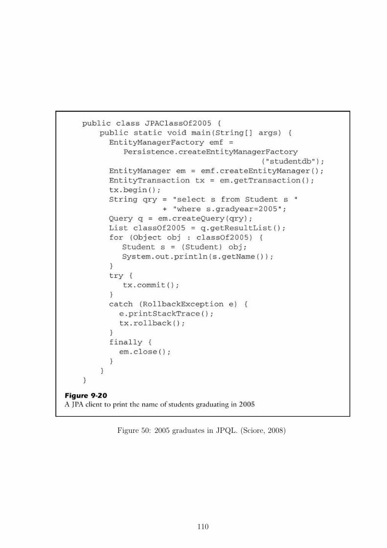
Figure 50: 2005 graduates in JPQL. (Sciore, 2008)

110

· Fetch the required persistent objects and process them as necessary.This processing may fetch other persistent objects invisibly.

¸ Commit the ORM transaction and forget the objects.That is, permit the corresponding Java objects be garbage collected by nolonger having references to them.

– Moreover, each such cycle should be as short as possible:

Just moving from one consistent state of the persistent data into the next –like an ordinary transaction.

– This is because a transaction prevents other concurrently running applicationprograms from accessing the same data – recall Isolation.

• This is one example of a general tradeoff in programming:

It is often straightforward to write code which is

either declarative

or resource-conscious

but hard to achieve both at the same time.

• The next big step from ORMs would be to switch from an RDBMS into a fullObject-Oriented DBMS (OODBMS) (Abiteboul et al., 1995, Chapter 21) (Connollyand Begg, 2010, Chapter 27).

– They look very promising when the data has such a complicated structurewhich calls for detailed OO design, as in Computer-Aided Design (CAD), Man-ufacturing (CAM), Software Engineering (CASE),. . .

– However, although OO is now the mainstream in programming methodology,and it has the impedance mismatch with RDBMS, OODBMS have remaineda niche commercially.

– One reason could be that although it is straightforward to move your datafrom one RDBMS into another, it may be much harder to move it from oneOODBMS into another — an organization might find itself stuck with just oneOODBMS vendor.

– Another could be that the SQL:1999 standard added some OO features (butnot many, to remain backwards compatible).

– Many RDBMS (such as Oracle 11g) have also added some OO features tobecome Object-Relational DBMS (ORDBMS) which offer a smaller step thanfull OODBMS.

– This course does not consider the wide and fragmented OODBMS field.

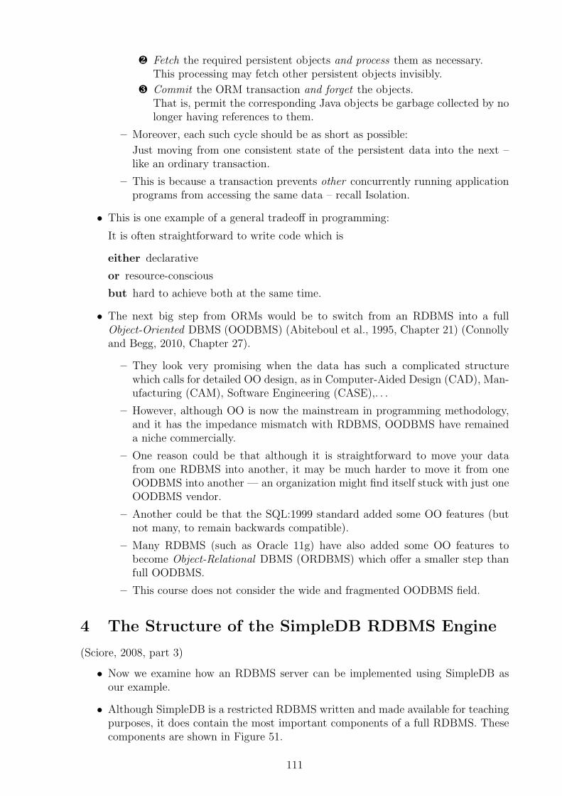
4 The Structure of the SimpleDB RDBMS Engine

(Sciore, 2008, part 3)

• Now we examine how an RDBMS server can be implemented using SimpleDB asour example.

• Although SimpleDB is a restricted RDBMS written and made available for teachingpurposes, it does contain the most important components of a full RDBMS. Thesecomponents are shown in Figure 51.

111

Figure 51: The components of an RDBMS engine. (Sciore, 2008, page 310)

• SimpleDB has chosen straightforward implementations for these components. Weshall mention some alternatives too.

• We can trace the execution of an SQL query in the SimpleDB RDBMS server processdown these components:

¶ The Remote manager handles the communication with the client. The serverprocess allocates a separate thread for each connection via the RMI meacha-nism.

· When a clients sends an SQL statement to its open connection, this Remotemanager passes it to the Planner component.

– This component plans how the statement will be executed.

– This plan is a Relational Algebra expression which it sends to the Querycomponent.

112

– It invokes the Parser component, which turns the statement into a syntaxtree containing the tables, attributes, constants,. . . mentioned in it.

– This Parser component in turn invokes the Metadata manager, whichkeeps track of information about the tables, attributes, indexes,. . . CRE-ATEd in the database to check that the things mentioned in the syntaxtree do exist and have the right type.

¸ The Query component turns the plan it received from the Planner componentinto a scan and executes it.

– It forms this scan by choosing an implementation for each operation inthe expression. For instance, if the expression contains a sort operation,then this Query component chooses a particular sorting algorithm to use.

– The RDBMS can choose from several algorithms for the same operation,because different algorithms suit different situations, improving perfor-mance.

– This component uses the Metadata manager too, because its informationhelps in making these choices.

– This scan is executed using the same “current row” approach as the clientuses for processing the result in its phase ® in section 3.2.

¹ Each of these rows processed by the Query component is stored on disk as arecord handled by the Record manager.

– These records are stored in disk blocks held in files managed by the Filemanager.

– The Buffer manager is in turn responsible for those disk blocks which havebeen read into RAM for accessing the records in them.

º Each (scan for a) statement is executed as (if in autocommit mode) or within(otherwise) a Transaction. They are managed by a manager responsible for

concurrency control and

recovery using a designated Log file managed by its own component.

• The relative order of these components may vary according to architecture:

– SimpleDB handles concurrency in the Buffer level, so its Transaction manageris located just above it.

– Other databases handle it in the Record level instead, and so their Transactionmanagers are above it instead.

• However, we will go upwards in Figure 51 so that each component

uses services provided by the components below it

provides services to the components above it.

4.1 File Management

(Sciore, 2008, Chapter 12)

• This lowest level of an RDBMS is the component which handles interaction withthe underlying disk drive(s).

• The RDBMS can do this with

113

raw disk(s) so that the database resides on dedicated drives (or partitions) withnothing else.

+ This is as fast as possible, but. . .

− such disks needs dedicated special support from the DBA.

This is used only for very high performance requirements.

OS file(s) so that the database is in normal files in normal file systems.

+ They need only the same support as file systems in general, but. . .

− the OS layer overhead impairs performance.

This is currently the most common choice.

• This OS file choice can be divided further into

single file architecture, where the whole database is stored in a single (possiblyvery) big file, like for instance the .mdb files of Microsoft Access.

multifile architecture, where each database is in a separate subdirectory containingseparate files for its tables, indexes,. . . like for instance Oracle and SimpleDBdo.

• The RDBMS treats its files internally like raw disks:

– It consults the OS only for opening and closing its files, and extending the withmore blocks, but. . .

– manages these blocks, their buffering, and their allocation by itself.

The reason is not only better performance but even more importantly ensuringdurability:

The RDBMS must know precisely which of its data is

already stored on disk, and which is

still only in RAM, and vanishes if the computer crashes.

Disks are persistent storage.

• In order to guarantee durability, the RDBMS needs some memory whose contentsdo not disappear when the computer crashes.

• A disk drive provide such persistent storage.

• A disk drive consists of sectors which the OS divides further into blocks.

• Big databases require big disks.

− Big disks are more expensive than small disks.

+ It is possible to connect many small disks into one unit, which looks like a bigdisk to the OS, because the controller of the unit takes care of spreading thestored data among these disks.

• Disk striping builds such a big disk out of many smaller disks. For performancereasons, it spreads the sectors of the big disk evenly across the sectors of the smallerdisks, as in Figure 52.

114

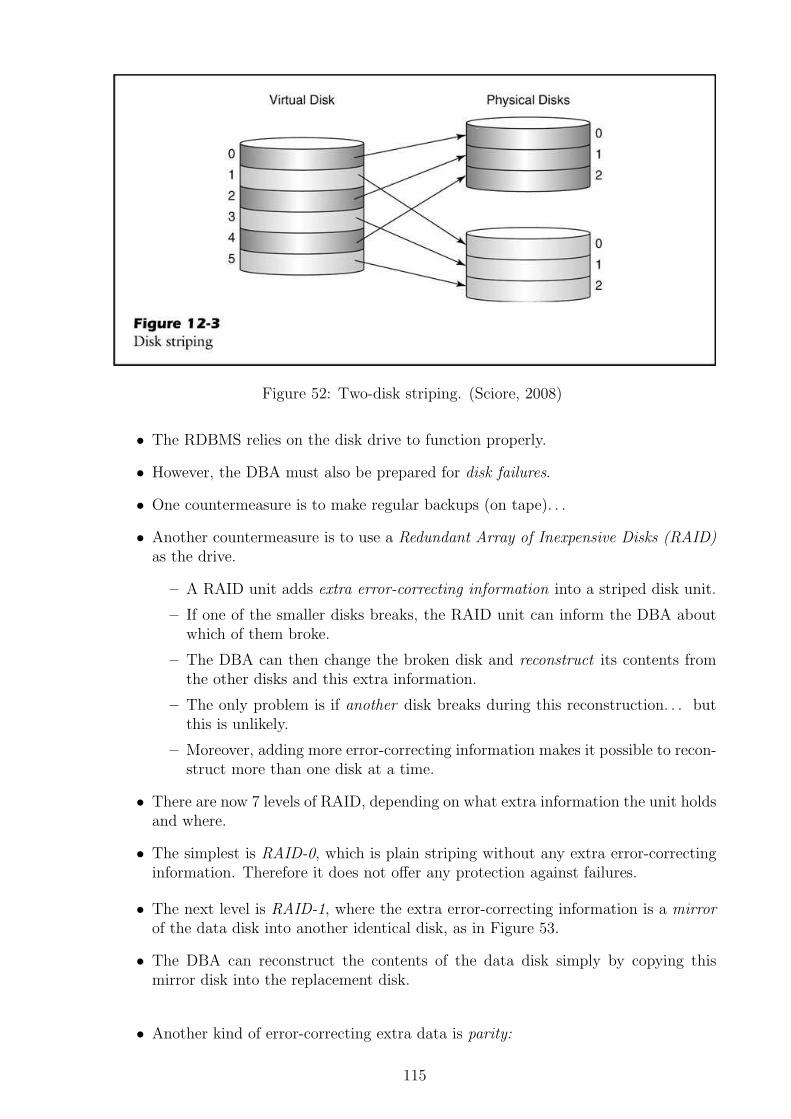
Figure 52: Two-disk striping. (Sciore, 2008)

• The RDBMS relies on the disk drive to function properly.

• However, the DBA must also be prepared for disk failures.

• One countermeasure is to make regular backups (on tape). . .

• Another countermeasure is to use a Redundant Array of Inexpensive Disks (RAID)as the drive.

– A RAID unit adds extra error-correcting information into a striped disk unit.

– If one of the smaller disks breaks, the RAID unit can inform the DBA aboutwhich of them broke.

– The DBA can then change the broken disk and reconstruct its contents fromthe other disks and this extra information.

– The only problem is if another disk breaks during this reconstruction. . . butthis is unlikely.

– Moreover, adding more error-correcting information makes it possible to recon-struct more than one disk at a time.

• There are now 7 levels of RAID, depending on what extra information the unit holdsand where.

• The simplest is RAID-0, which is plain striping without any extra error-correctinginformation. Therefore it does not offer any protection against failures.

• The next level is RAID-1, where the extra error-correcting information is a mirrorof the data disk into another identical disk, as in Figure 53.

• The DBA can reconstruct the contents of the data disk simply by copying thismirror disk into the replacement disk.

• Another kind of error-correcting extra data is parity:

115

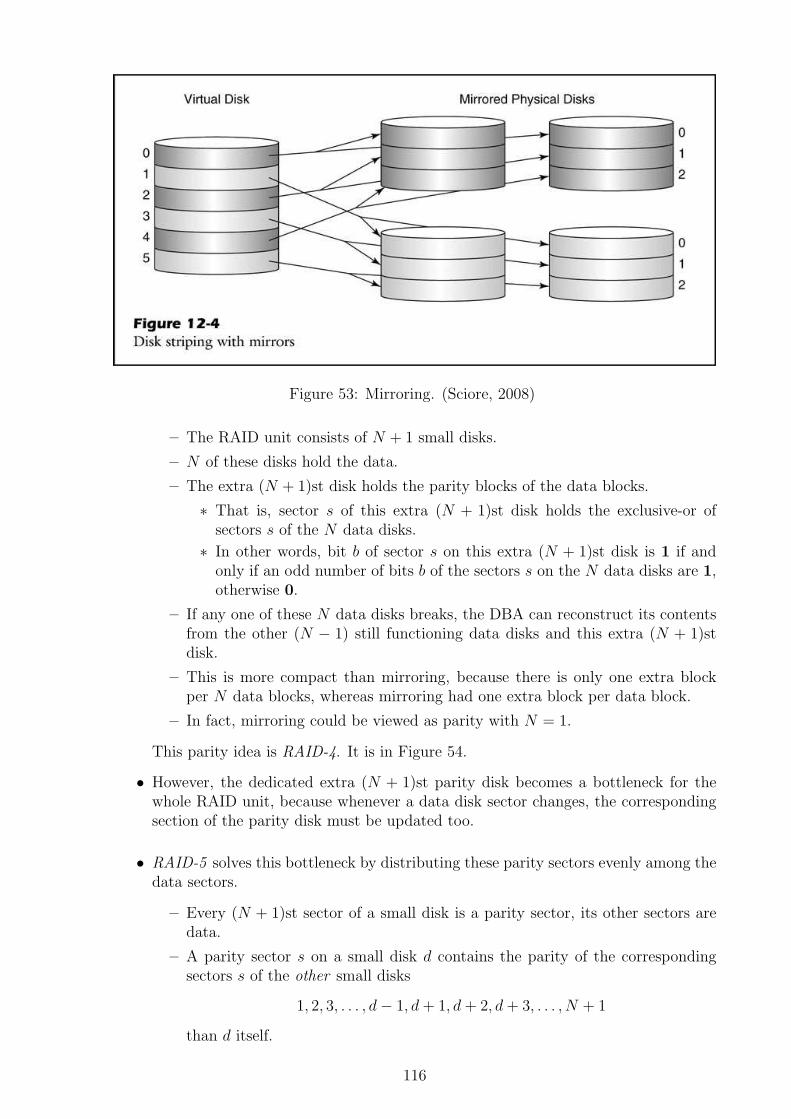
Figure 53: Mirroring. (Sciore, 2008)

– The RAID unit consists of N + 1 small disks.

– N of these disks hold the data.

– The extra (N + 1)st disk holds the parity blocks of the data blocks.

∗ That is, sector s of this extra (N + 1)st disk holds the exclusive-or ofsectors s of the N data disks.

∗ In other words, bit b of sector s on this extra (N + 1)st disk is 1 if andonly if an odd number of bits b of the sectors s on the N data disks are 1,otherwise 0.

– If any one of these N data disks breaks, the DBA can reconstruct its contentsfrom the other (N − 1) still functioning data disks and this extra (N + 1)stdisk.

– This is more compact than mirroring, because there is only one extra blockper N data blocks, whereas mirroring had one extra block per data block.

– In fact, mirroring could be viewed as parity with N = 1.

This parity idea is RAID-4. It is in Figure 54.

• However, the dedicated extra (N + 1)st parity disk becomes a bottleneck for thewhole RAID unit, because whenever a data disk sector changes, the correspondingsection of the parity disk must be updated too.

• RAID-5 solves this bottleneck by distributing these parity sectors evenly among thedata sectors.

– Every (N + 1)st sector of a small disk is a parity sector, its other sectors aredata.

– A parity sector s on a small disk d contains the parity of the correspondingsectors s of the other small disks

1, 2, 3, . . . , d − 1, d + 1, d + 2, d + 3, . . . , N + 1

than d itself.

116

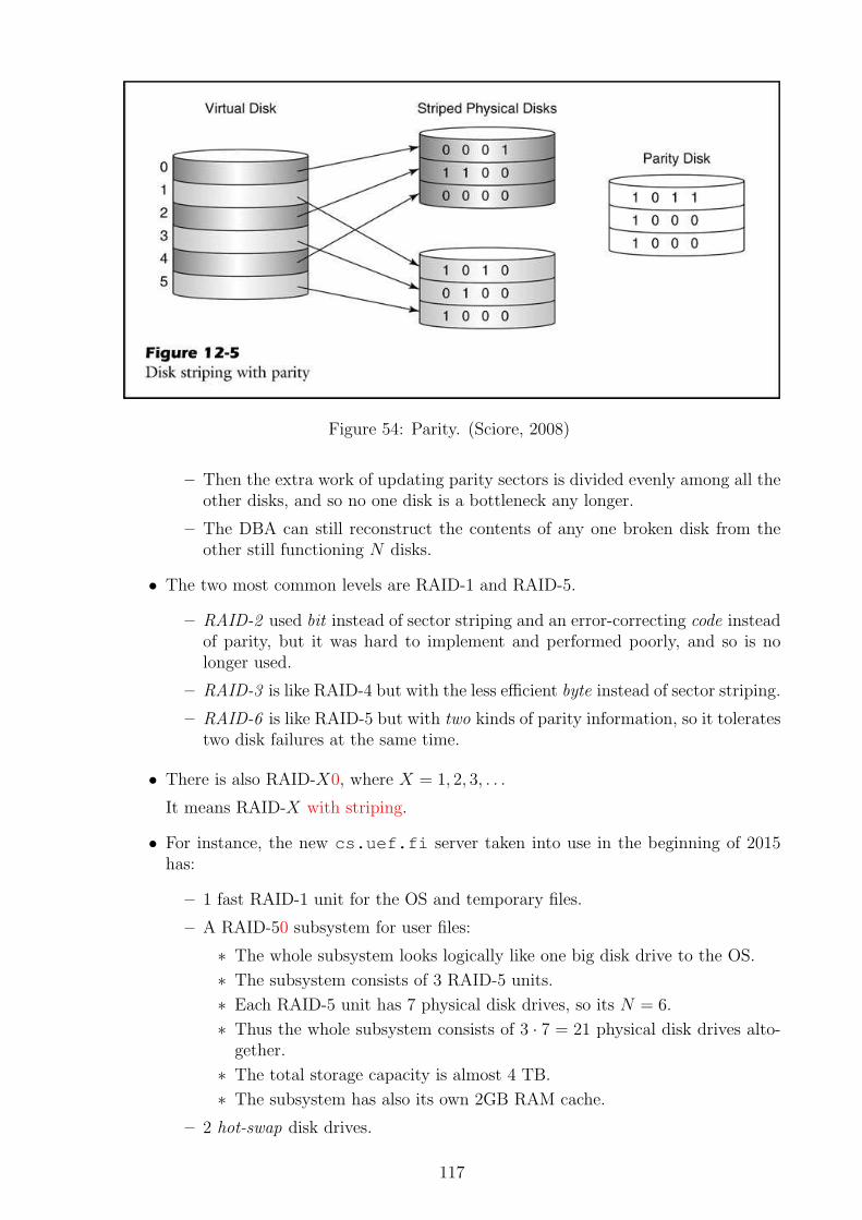
Figure 54: Parity. (Sciore, 2008)

– Then the extra work of updating parity sectors is divided evenly among all theother disks, and so no one disk is a bottleneck any longer.

– The DBA can still reconstruct the contents of any one broken disk from theother still functioning N disks.

• The two most common levels are RAID-1 and RAID-5.

– RAID-2 used bit instead of sector striping and an error-correcting code insteadof parity, but it was hard to implement and performed poorly, and so is nolonger used.

– RAID-3 is like RAID-4 but with the less efficient byte instead of sector striping.

– RAID-6 is like RAID-5 but with two kinds of parity information, so it toleratestwo disk failures at the same time.

• There is also RAID-X0, where X = 1, 2, 3, . . .

It means RAID-X with striping.

• For instance, the new cs.uef.fi server taken into use in the beginning of 2015has:

– 1 fast RAID-1 unit for the OS and temporary files.

– A RAID-50 subsystem for user files:

∗ The whole subsystem looks logically like one big disk drive to the OS.

∗ The subsystem consists of 3 RAID-5 units.

∗ Each RAID-5 unit has 7 physical disk drives, so its N = 6.

∗ Thus the whole subsystem consists of 3 · 7 = 21 physical disk drives alto-gether.

∗ The total storage capacity is almost 4 TB.

∗ The subsystem has also its own 2GB RAM cache.

– 2 hot-swap disk drives.

117

∗ They allow the IT staff to plug in a new physical disk drive without havingto shut down the whole server.

∗ Thus they can reconstruct a broken physical disk drive “on the fly”.

• The IT support (including the DBAs) recommends which RAID to buy based onthe required levels of

protection against downtime and loss of work caused by disk failures – in theory,by determining a low enough expected value

disk failure probability · cost of disk failure

of the cost involved – and

performance requirements for the system – based on

statistics collected about its current use, and

estimates about its future use.

Disks are slow.

• Disk storage is much slower than RAM: About

100 000 times slower for mechanical disk drives, but “only” about

1 000 times slower for flash drives.

Requirement 11 (little I/O). The RDBMS must strive to avoid unnecessary disk I/Owhenever possible.

• This is one reason why the RDBMS executes queries concurrently:

If one query running in one thread must stop and wait for disk I/O, other queriesrunning in other threads which already have the data they need in RAM maycontinue.

Disks are block devices.

• Disk storage is different from RAM also in that its addressing operates in muchlarger units than single bytes.

• Each disk drive / file system / OS has its own block size constant, so that the blockk = 0, 1, 2, . . . of a file consists of the bytes at

from k · block size into (k + 1) · block size − 1

within that file, and reading/writing the value of any byte within that area copiesthe whole block between disk and RAM.

• One way how the RDBMS can meet requirement 11 is to ensure that if a block mustbe read from the disk, then the information in it is used as well as possible.

• This constant is usually between 512 bytes and 16 kilobytes, 4 kilobytes is a typicalvalue.

118

• On the one hand, the application programmer does not have to be aware of thisbuffering because the OS handles it.

But (s)he may want to be, for performance reasons.

• On the other hand, the RDBMS wants to be aware of it, and bypasses this OSbuffering altogether with its own Buffer manager, for both performance and dura-bility.

• That Buffer manager will use the services offered by this File manager for the actualdisk I/O operations.

+ SimpleDB source file simpledb/file/Block.java

• A Block object represents logical block number: a block number k within a particularOS file.

• The OS converts it internally into a physical block number, which identifies a par-ticular block on a particular sector of the disk drive.

+ SimpleDB source file simpledb/file/Page.java

• A Page object is a Block -sized chunk of memory.

• It is implemented with library class Java.nio.ByteBuffer .

• This library class provides also a reading/writing position within the chunk.

• Moreover, a Page object allocates the chunk Direct ly:

– This means that Java uses one of its OS I/O buffers as the chunk.

– This is a good idea in an RDBMS (but not in most other programming situa-tions!) because it will manage its own Buffers.

– In this way, the RDBMS can “recycle” the same memory which the OS wouldhave used for the same purpose.

• All these methods (like many others) are synchronized (Sestoft, 2005, Chap-ter 16.2):

– That is, only one thread can execute the methods of a Page object at the sametime.

– Because the RDBMS process handles each connection with a client in its ownthread, this ensures that two clients cannot manipulate the same Page at thesame time – one must wait until the other is finished instead.

– This is important for the get. . . and set. . . methods, which

¬ first move the position where they want it to be, and

­ then read or write the data starting at that position.

119

+ SimpleDB source file simpledb/file/FileMgr.java

• The SimpleDB process has just one global File Manager object. It handles all diskI/O operations

read the contents of Block from disk into a ByteBuffer – for instance, into a Pageobject

write a ByteBuffer into an already existing disk Block

append a new Block into the end of a file

get size of a file as the number of disk blocks in it

for the other components.

• It also opens all requested files and keeps them in openFiles to avoid reopeningthem.

• These files are opened in binary random access

read and

write and

synchronous so that when write is executed without errors, then the operationhas really modified this block of this file on disk – this is where the RDBMStakes over Buffer ing from the OS.

mode.

4.2 Log Management

(Sciore, 2008, Chapters 13.1–13.3)

• The RDBMS has two kinds of files:

Data files (and their supporting files like indexes, metadata,. . . ) – the RDBMShas only partial control over their access patterns, because they depend on theusers’ queries too

Log file – which the RDBMS controls fully. It is. . .

– an extremely important special file, because it is the central concept toimplement database recovery after a crash!

– a “diary” (or “ship’s log” or “journal”) of all the operations which theRDBMS has performed recently.

• You have (most likely. . . ) already encountered these log files implicitly in your dailywork:

– For instance, when Microsoft Word crashes, and is restarted, then it may ask“Do you want to recover your file?”

– It can do this, because it has kept a log of all operations since the last “Save”operation, and so it can redo them.

• Because this Log file is so important, and the RDBMS processes it differently fromits other files, it has its own manager.

120

• The Log file consists of log records.

– Each log record is identified with a Log Sequence Number (LSN).

– Each RDBMS operation generates its own kind of log record. The basic prin-ciple is:

Suppose this Transaction is aborted later. Is this operation somethingthat you must undo then? If it is, then write a log record about itwhen you do it! So that you remember to undo it.

– These log records are written at the end of the log in the order in which theRDBMS executes their operations – that is, “forward in time”.

– However, recovery needs to read the Log file not only forward but also backwardsin time – also from the most recently written log record at the end towards theolder log records at the beginning.

– Hence the Log file is a linked list of log records, where each record has also abackward pointer to the previous one.

• The RDBMS allocates a specific Page which represents the last block of the Log file(step 1 in Figure 55).

– All the previous blocks of the Log file have aready been written onto the disk.

– This last block may or may not have been written onto the disk yet.

• The log grows with the operations

append a new log record at the end of the Log file (step 2 in Figure 55) and giveit an LSN

flush a given LSN (step 3 in Figure 55) – that is, make sure that it is reallywritten onto the disk, and not just on the last log Page in RAM

which write the last log Page onto the disk if necessary.

• Since only the last log Page is still in RAM, flushing an LSN implies flushingall the log records before it as well.

• The algorithm in Figure 55 is optimal in the sense that it writes the last log Pageonto the disk only when

append finds that it is already full, or

flush commands it to write an LSN in it.

• However, the algorithm in Figure 55 may write the same last log Page many times:

– once for each flush in it, and

– once more for the last append which finds it full.

• The algorithm in Figure 55 can be further improved to write each last log Page(almost) just once with some concurrent programming:

– When a thread flushes an LSN in the last log Page, then it goes to sleepwaiting for some other thread to write the Page. It is namely enough to havethe LSN on disk when this flushing thread continues.

121