1

3.3 LIMB CORRECTION OF INFRARED IMAGERY IN CLOUDY REGIONS FOR THE IMPROVED INTERPRETATION OF RGB COMPOSITES

Nicholas J. Elmer1,4,*, Emily Berndt2,4, Gary J. Jedlovec3,4

1Department of Atmospheric Science, University of Alabama in Huntsville, Huntsville, Alabama, USA 2Earth System Science Center, University of Alabama in Huntsville, Huntsville, Alabama, USA 3Earth Science Office, NASA Marshall Space Flight Center (MSFC), Huntsville, Alabama, USA

4NASA Short-term Prediction Research and Transition (SPoRT) Center, Huntsville, Alabama, USA

1. INTRODUCTION

Red-Green-Blue (RGB) composites (EUMETSAT User Services 2009) combine information from several channels into a single composite image. RGB composites contain the same information as the original channels, but presents the information in a more efficient manner. However, RGB composites derived from infrared imagery of both polar-orbiting and geostationary sensors are adversely affected by the limb effect, which interferes with the qualitative interpretation of RGB composites at large viewing zenith angles.

The limb effect, or limb-cooling, is a result of an increase in optical path length of the absorbing atmosphere as viewing zenith angle increases (Goldberg et al. 2001; Joyce et al. 2001; Liu and Weng 2007). As a result, greater atmospheric absorption occurs at the limb, causing the sensor to observe anomalously cooler brightness temperatures. Figure 1 illustrates this effect. In general, limb-cooling results in a 4-11 K decrease in measured brightness temperature (Liu and Weng 2007) depending on the infrared band. For example, water vapor and ozone absorption channels display much larger limb-cooling than infrared window channels. Consequently, RGB composites created from infrared imagery not corrected for limb effects can only be reliably interpreted close to nadir, which reduces the spatial coverage of the available imagery.

Elmer (2015) developed a reliable, operational limb correction technique for clear regions. However, many RGB composites are intended to be used and interpreted in cloudy regions, so a limb correction methodology valid for both clear and cloudy regions is needed. This paper presents a limb correction technique valid for both clear and cloudy regions, which is described in Section 2. Section 3 presents

several RGB case studies demonstrating the improved functionality of limb-corrected RGBs in both clear and cloudy regions, and Section 4 summarizes and presents the key conclusions of this work.

2. LIMB CORRECTION Following the methodology in Elmer (2015), limb

correction coefficients, which describe the change in brightness temperature due to limb effects, were derived from the Joint Center for Satellite Data Assimilation (JCSDA) Community Radiative Transfer Model (CRTM; Han et al. 2006) for the Suomi-NPP Visible Infrared Imaging Radiometer Suite (VIIRS), Meteosat Second Generation (MSG) Spinning Enhanced Visible and Infrared Imager (SEVIRI), and Advanced Himawari Imager (AHI) infrared bands. Limb correction coefficients for Aqua and Terra Moderate Resolution Imaging Spectroradiometer were obtained directly from Elmer (2015). Note that the limb correction coefficients vary both latitudinally and

* Corresponding author address: Nicholas J. Elmer, Univ.

of Alabama in Huntsville, Dept. of Atmospheric Sciences,

Huntsville, AL 35805, phone: 256-961-7356, email:

nicholas.j.elmer@nasa.gov.

Figure 1. As the satellite scans from nadir to the limb, the

optical path length of the absorbing atmosphere

increases, resulting in limb-cooling.

https://ntrs.nasa.gov/search.jsp?R=20160001851 2018-07-16T13:29:27+00:00Z

2

seasonally, similar to the findings of Joyce et al. (2001), and were derived assuming a clear sky.

In cloudy regions, clouds impact the observed limb-cooling, since cloudy scenes have a shorter optical path length than clear scenes. Therefore, if limb effects are corrected without accounting for clouds, the limb correction will be inaccurate in cloudy regions. To develop the limb correction for cloudy regions, layer optical thickness (τl) was obtained from CRTM for MODIS, VIIRS, SEVIRI, and AHI using the same model atmospheric profiles from Elmer (2015). Layer optical thickness was converted to atmospheric transmittance from cloud top pressure (p) to the top-of-atmosphere (TOA), t(p), where,

𝑡(𝑝) = 𝑡𝑙(𝑝) 𝑡(𝑝 − 1) (1) and

𝑡𝑙(𝑝) = 𝑒−𝜏𝑙(𝑝). (2) t(p) was then normalized by the total atmospheric transmittance,

𝑄(𝑝) =𝑡(0)−𝑡(𝑝)

𝑡(0)−𝑡(𝑝𝑠), (3)

where the normalized value, Q, which also varies latitudinally and seasonally, is defined as the cloud correction coefficient. Note that Q decreases as p

decreases, so Q = 1 for clear regions, whereas Q < 1 for cloudy regions.

Modifying the limb correction equation from Elmer (2015) to include Q, and ignoring channel differences between sensors, results in

TCORR = TB + Q [C2 ln(cosθZ)2 − C1 ln(cosθZ)], (4)

where TCORR is the limb corrected brightness temperature, TB is the original measured brightness temperature, Q is the cloud correction coefficient, C1 and C2 are limb correction coefficients, and θZ is the viewing zenith angle. Note that Q is a function of cloud top pressure, so a cloud product is needed to properly apply the limb correction in cloudy regions.

The limb correction equation (Eq. 4) is applied to individual infrared bands prior to creating the RGB composite to remove limb effects, and is valid for both polar-orbiting and geostationary sensors. More information about the limb correction equation valid for clear and cloudy regions can be found in Elmer et al. (2016). 3. RESULTS AND DISCUSSION

Figure 2 shows the impact of limb correction on reducing errors in brightness temperature due to limb-

Figure 2. 1330 UTC 28 June 2015 Aqua MODIS band 27 (6.7 μm) minus SEVIRI band 5 (6.2 μm) brightness temperature

difference for (left) uncorrected and (right) limb-corrected water vapor imagery. Color scale in Kelvin.

3

cooling. In the uncorrected imagery, anomalous cooling of 6-8 K is observed along the edge of the MODIS swath. However, in the corrected imagery, the anomalous cooling is removed, and brightness temperature differences (BTDs) of less than ±2 K are observed. Large differences are observed near cloudy regions due to differences in viewing angle and cloud movement between the MODIS and SEVIRI observation times.

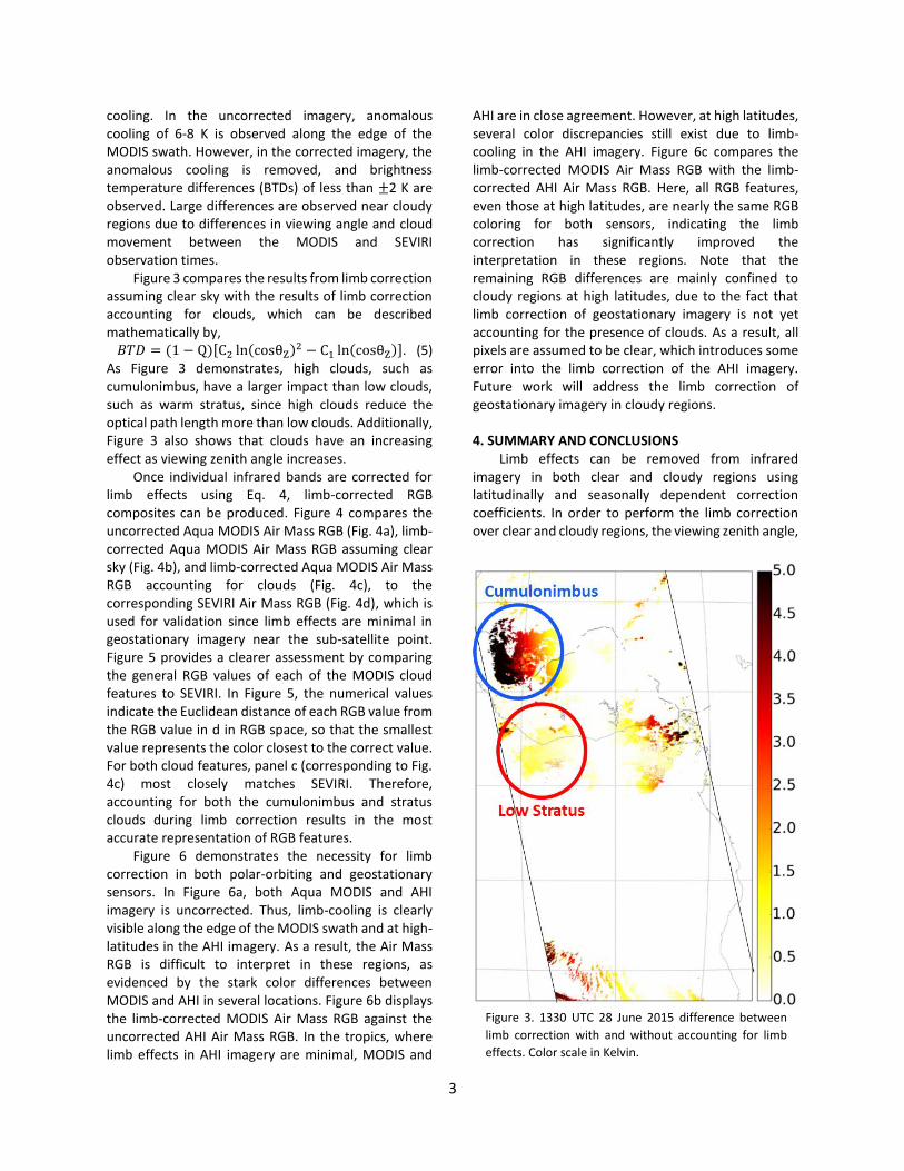
Figure 3 compares the results from limb correction assuming clear sky with the results of limb correction accounting for clouds, which can be described mathematically by, 𝐵𝑇𝐷 = (1 − Q)[C2 ln(cosθZ)

2 − C1 ln(cosθZ)]. (5) As Figure 3 demonstrates, high clouds, such as cumulonimbus, have a larger impact than low clouds, such as warm stratus, since high clouds reduce the optical path length more than low clouds. Additionally, Figure 3 also shows that clouds have an increasing effect as viewing zenith angle increases.

Once individual infrared bands are corrected for limb effects using Eq. 4, limb-corrected RGB composites can be produced. Figure 4 compares the uncorrected Aqua MODIS Air Mass RGB (Fig. 4a), limb-corrected Aqua MODIS Air Mass RGB assuming clear sky (Fig. 4b), and limb-corrected Aqua MODIS Air Mass RGB accounting for clouds (Fig. 4c), to the corresponding SEVIRI Air Mass RGB (Fig. 4d), which is used for validation since limb effects are minimal in geostationary imagery near the sub-satellite point. Figure 5 provides a clearer assessment by comparing the general RGB values of each of the MODIS cloud features to SEVIRI. In Figure 5, the numerical values indicate the Euclidean distance of each RGB value from the RGB value in d in RGB space, so that the smallest value represents the color closest to the correct value. For both cloud features, panel c (corresponding to Fig. 4c) most closely matches SEVIRI. Therefore, accounting for both the cumulonimbus and stratus clouds during limb correction results in the most accurate representation of RGB features.

Figure 6 demonstrates the necessity for limb correction in both polar-orbiting and geostationary sensors. In Figure 6a, both Aqua MODIS and AHI imagery is uncorrected. Thus, limb-cooling is clearly visible along the edge of the MODIS swath and at high-latitudes in the AHI imagery. As a result, the Air Mass RGB is difficult to interpret in these regions, as evidenced by the stark color differences between MODIS and AHI in several locations. Figure 6b displays the limb-corrected MODIS Air Mass RGB against the uncorrected AHI Air Mass RGB. In the tropics, where limb effects in AHI imagery are minimal, MODIS and

AHI are in close agreement. However, at high latitudes, several color discrepancies still exist due to limb-cooling in the AHI imagery. Figure 6c compares the limb-corrected MODIS Air Mass RGB with the limb-corrected AHI Air Mass RGB. Here, all RGB features, even those at high latitudes, are nearly the same RGB coloring for both sensors, indicating the limb correction has significantly improved the interpretation in these regions. Note that the remaining RGB differences are mainly confined to cloudy regions at high latitudes, due to the fact that limb correction of geostationary imagery is not yet accounting for the presence of clouds. As a result, all pixels are assumed to be clear, which introduces some error into the limb correction of the AHI imagery. Future work will address the limb correction of geostationary imagery in cloudy regions. 4. SUMMARY AND CONCLUSIONS

Limb effects can be removed from infrared imagery in both clear and cloudy regions using latitudinally and seasonally dependent correction coefficients. In order to perform the limb correction over clear and cloudy regions, the viewing zenith angle,

Figure 3. 1330 UTC 28 June 2015 difference between

limb correction with and without accounting for limb

effects. Color scale in Kelvin.

4

latitude, and cloud top pressure for each image pixel is required.

As was shown by the RGB cases in Section 3, limb-corrected RGB composites increase the confidence in the interpretation of RGB features and improve the situational awareness of operational forecasters using the corrected RGB composite. The limb correction technique described in this paper can be easily applied to future infrared sensors, including the Geostationary Operational Environmental Satellite R-Series (GOES-R)

Advanced Baseline Imager (ABI) in order to create limb-corrected RGB composites as soon as imagery becomes available. REFERENCES Elmer, N. J., E. Berndt, and G. Jedlovec, 2016: Limb

correction of MODIS and VIIRS infrared channels for the improved interpretation of RGB composites. Accepted with minor revisions, J. Atmos. Ocean. Tech.

Figure 4. 1330 UTC 28 June 2015 (a) uncorrected, (b) limb-corrected assuming clear sky, (c) limb corrected accounting for

clouds Aqua MODIS Air Mass RGB overlaying (d) the corresponding SEVIRI Air Mass RGB.

5

Elmer, N. J., 2015: Limb correction of individual infrared channels for the improved interpretation of RGB composites. M.S. thesis, Department of Atmospheric Science, Univ. of Alabama in Huntsville, 75 pp.

EUMETSAT User Services, 2009: Best practices for RGB compositing of multi-spectral imagery. Darmstadt, 8 pp., http://oiswww.eumetsat.int/~idds/html/doc/best_practices.pdf.

Goldberg, M. D., D. S. Crosby, and L. Zhou, 2001: The limb adjustment of AMSU-A observations: Methodology and validation. J. Appl. Meteor., 40, 70-83.

Han, Y., P. van Delst, Q. Liu, F. Weng, B. Yan, R. Treadon, and J. Derber, 2006: JCSDA Community Radiative Transfer Model (CRTM). Tech. rep., Washington, D.C.

Joyce, R., J. Janowiak, and G. Huffman, 2001: Latitudinally and seasonally dependent zenith-angle corrections for geostationary satellite IR brightness temperatures. J. Appl. Meteor., 40, 689-703.

Liu, Q. and F. Weng, 2007: Uses of NOAA-16 and -18 satellite measurements for verifying the limb-correction algorithm. J. Appl. Meteor. Climatol., 46, 544-548.

Figure 5. General RGB values of the cloud features

indicated in Fig. 4. Panels a-d correspond to the same

panels in Fig. 4 for both cloud features, and the numerical

values represent the Euclidean distance of the RGB value

in (a-c) from the RGB value in (d) in RGB color space.

Figure 6. 1640 UTC 21 October 2015 (left) uncorrected Aqua MODIS and uncorrected AHI Air Mass RGB, (center) limb-

corrected Aqua MODIS and uncorrected AHI Air Mass RGB, and (right) limb-corrected Aqua MODIS and limb-corrected AHI

Air Mass RGB. Color insets compare the RGB coloring between the MODIS and AHI.