3496 ieee transactions on wireless ......3496 ieee transactions on wireless communications, vol. 12,...

3496 IEEE TRANSACTIONS ON WIRELESS COMMUNICATIONS, VOL. 12, NO. 7, JULY 2013

Optimal Tradeoff Between Sum-Rate Efficiency andJain’s Fairness Index in Resource Allocation

Akram Bin Sediq, Student Member, IEEE, Ramy H. Gohary, Senior Member, IEEE, Rainer Schoenen,and Halim Yanikomeroglu, Senior Member, IEEE

Abstract—The focus of this paper is on studying the tradeoffbetween the sum efficiency and Jain’s fairness index in generalresource allocation problems. Such problems are frequentlyencountered in wireless communication systems with M users.Among the commonly-used methods to approach these problemsis the one based on the α-fair policy. Analyzing this policy, it isshown that it does not necessarily achieve the optimal Efficiency-Jain tradeoff (EJT) except for the case of M = 2 users. Whenthe number of users M > 2, it is shown that the gap betweenthe efficiency achieved by the α-fair policy and that achievedby the optimal EJT policy for the same Jain’s index can beunbounded. Finding the optimal EJT corresponds to solving afamily of potentially difficult non-convex optimization problems.To alleviate this difficulty, we derive sufficient conditions whichare shown to be sharp and naturally satisfied in various radioresource allocation problems. These conditions provide us with ameans for identifying cases in which finding the optimal EJTand the rate vectors that achieve it can be reformulated asconvex optimization problems. The new formulations are used todevise computationally-efficient resource schedulers that enablethe optimal EJT to be achieved for both quasi-static and ergodictime-varying communication scenarios. Analytical findings areconfirmed by numerical examples.

Index Terms—Scheduling, convex optimization, α-fairness,fairness metrics, efficiency-fairness tradeoff.

I. INTRODUCTION

THE resources available for wireless communication sys-tems are usually scarce and shared among multiple users.

The way in which these resources are allocated determinesthe efficiency of the system and the benefits received by itsusers. Since the service provider is interested in maximizingthe efficiency of the system and the users are interested inmaximizing their own benefits, the allocation of resourcesis typically encountered by conflicting goals. For instance,favouring a certain class of users may increase the systemefficiency, but would result in the dissatisfaction of otherclasses of users. In contrast, providing equal benefits to allusers yields higher fairness, but will potentially result in lowefficiency. To control the emphasis placed on various goals, the

Manuscript received November 2, 2012; revised February 8 and April 15,2013; accepted April 15, 2013. The associate editor coordinating the reviewof this paper and approving it for publication was D. Niyato.

The authors are with the Department of Systems and Computer Engineer-ing, Carleton University, Ottawa, ON, Canada (e-mail: {akram, gohary, rs,halim}@sce.carleton.ca).

This work is supported in part by Huawei Technologies Canada Co., Ltd.,in part by the Natural Sciences and Engineering Research Council (NSERC)of Canada, and in part by the Ontario Graduate Scholarship (OGS).

A preliminary version of this work was presented at the 2012 IEEE Int.Symp. Personal, Indoor and Mobile Radio Commun. (PIMRC’12).

Digital Object Identifier 10.1109/TWC.2013.061413.121703

provider uses a tradeoff policy, which, unless properly chosen,can result in wasteful allocation of resources. In particular, asuboptimal tradeoff policy can be less efficient and, at thesame time, less fair to the users [1]–[3].

The benefits received by the users in the downlink ofa wireless communication system can be measured by therates at which data is delivered to these users. These ratesare controlled by appropriate allocation of radio resources atthe transmitter. For instance, the transmitter may allocate itsresources in such a way that maximizes the sum of the ratesdelivered to the users. This allocation favours users that aregeographically closer to the transmitter, but “starves” fartherusers. Although more efficient from the system perspective,such an allocation is unfair to the users at less advantageouslocations [4], [5]. A fairer allocation is one in which theminimum rate received by the users is maximized [1], [3],[6]. However, this allocation can result in unacceptable systemefficiency, i.e., low sum-rate. Hence, it is desirable to find anoptimal tradeoff policy whereby the system provider allocatesits resources in such a way that no other allocation can providea strictly higher efficiency and at the same time be fairer tothe users. The focus of this paper is two-fold: 1) to develop atechnique for obtaining an efficiency-fairness tradeoff that isoptimal in a specific sense; and 2) to derive sufficient condi-tions, which, when satisfied by the set of feasible benefits, leadto efficiently computable optimal tradeoff and benefit vectors.

The applications that we will consider herein are derivedfrom practical radio resource scheduling problems that arisein wireless communication systems operating over quasi-staticand ergodic time-varying channels. However, our analysisapplies to a broader class of frameworks, including social andeconomics ones [2], [7], [8].

To study the tradeoff between efficiency and fairness, wenote that efficiency is usually defined depending on the partic-ular resource allocation problem considered. For instance, inthe case of wireless networks considered herein, efficiencyis measured by the sum-rate delivered to the users of thenetwork. In contrast, several definitions are used to quantifyfairness. In [2], axioms that include continuity and homogene-ity, and subsequent features, are provided to obtain a generalclass of plausible fairness measures. Among the members ofthat class are the entropy-based index [2] and Jain’s fairnessindex [9]. In addition to the axioms and features providedin [2], we identify two more features that commend the useof Jain’s index as a fairness measure.

• Conformity to standard fairness benchmarks: A fairness

1536-1276/13$31.00 © 2013 IEEE

SEDIQ et al.: OPTIMAL TRADEOFF BETWEEN SUM-RATE EFFICIENCY AND JAIN’S FAIRNESS INDEX IN RESOURCE ALLOCATION 3497

measure with this feature can be related to easily conceiv-able benchmarks. For instance, a Jain’s index of p/100can be regarded as the fairness index of an equivalentresource allocation in which p% of the users receiveequal non-zero benefits and the remaining (100 − p)%receive zero benefits [9]. Analogous relations betweenother metrics and standard benchmarks are not readilyavailable.

• Accommodating more users: A good fairness measureenables more users with specific benefit requirements tobe accommodated in the system. The superiority of Jain’sindex in that respect will be illustrated by numericalcomparisons hereinafter.

A common approach to trading off efficiency with fair-ness in wireless networks, is to allocate the resources in away that maximizes the sum-rate efficiency while ensuringthat the minimum rates achieved by the users exceed someprescribed bounds, e.g., [3], [8]. Varying these bounds overthe set of feasible rates provides a means for controllingfairness [3]. Another approach is to allocate the resourcesin a way that maximizes a parametric utility, whereby oneor multiple parameters are used to control the emphasis onefficiency and fairness. A commonly used policy is the α-fair one (also known as the α-fair utility) [1], wherein varioussettings of a parameter α yield allocations that achieve popularefficiency-fairness tradeoffs. For instance, setting α = 0 yieldsmaximum efficiency, setting α = 1 yields proportionally fairallocations [10], and setting α =∞ yields allocations that arefair in the max-min sense [1]. Motivations for using the α-fairpolicy are provided in [2]. Generally speaking, increasing αresults in allocations that are fairer [2] in a sense that doesnot necessarily conform to Jain’s index, as will be shownhereinafter. Other parametric utilities for trading off efficiencyand fairness are considered in [11] and [12], and a comparisonbetween multiple tradeoff criteria is provided in [13].

Compared with other measures, Jain’s index provides afairness criterion that takes into consideration all the usersof the system, not only those users that are assigned minimalresources [9]. Maximizing Jain’s index without wasting valu-able resources requires optimal tradeoff between efficiencyand this index. A question that arises is whether maximizingthe well-studied α-fair policy yields such an optimal tradeoff.To address this question, we show that α-fair allocationsare not guaranteed to achieve the optimal Efficiency-Jaintradeoff (EJT) except for the case of M = 2 users. Toovercome this drawback, we develop a generic techniquefor obtaining optimal EJT allocations. Unfortunately, thistechnique involves solving potentially difficult non-convex op-timization problems. To alleviate this difficulty, we derive suf-ficient conditions, which are shown to be sharp and naturallysatisfied in various radio resource allocation problems. Theseconditions provide us with a means for identifying cases inwhich finding the optimal EJT and the rate vectors that achieveit can be reformulated as convex optimization problems. Thenew formulations are used to devise computationally-efficientresource schedulers that enable the optimal EJT to be achievedfor both quasi-static and ergodic time-varying communicationscenarios.

Numerical results are provided for confirming our theo-

retical findings and for demonstrating the advantage of theoptimal tradeoff provided by our technique over the α-fairone.

Notation: Bold-face and regular-face fonts will be usedto denote vectors and scalars, respectively. The set of length-M vectors with non-negative real entries will be denoted byR

M+ and the length-M all-one and all-zero vectors will be

denoted by 1M and 0M , respectively. The symbols � and �will be used to denote element-wise inequalities, and (·)T willbe used to denote the transpose. The Euclidean norm will bedenoted by ‖ · ‖.

II. PRELIMINARIES

Let x ∈ C ⊆ RM+ be a vector of non-negative real entries

{xm}Mm=1, where xm is the benefit received by user m andC is the set of feasible benefit vectors. Generally, the benefits{xm}Mm=1 and the set C depend on the application and theresources allocated to each user [9, Sec. 5]. For example,in the downlink of wireless communications, xm can be therate of user m resulting from a particular allocation of theradio resources, and C can be the set of all achievable rates.In this paper, the efficiency, η(x), of a resource allocation isdefined by the sum of benefits (i.e., η(x) =

∑Mm=1 xm), and

its fairness is given by the Jain’s index defined below.

Definition 1 (Jain’s Index [9]). For x ∈ RM+ , Jain’s fairness

index J : RM+ → R+ is given by

J(x) =( M∑m=1

xm

)2/M

M∑m=1

x2m. (1)

�This definition shows that J(x) is continuous and lies in[1M , 1

]. In this interval, J = 1

M corresponds to the least fairallocation in which only one user receives a non-zero benefit,and J = 1 corresponds to the fairest allocation in which allusers receive the same benefit.

In many cases, depending on C, there is an inherent tradeoffbetween η(x) and J(x). Hence, to ensure efficient utilizationof resources, we seek the optimal tradeoff, which is definednext.

Definition 2 (Optimal Efficiency-Jain tradeoff (EJT)). Anoptimal EJT is one that results in a benefit vector x� suchthat no x = x�, x ∈ C satisfies either: 1) η(x) > η(x�), andat the same time, J(x) ≥ J(x�), or 2) η(x) ≥ η(x�), and atthe same time, J(x) > J(x�). �

This definition is closely related to Pareto optimality definedfor optimization problems with multiple objectives [14]. Withefficiency and Jain’s index as objectives, a Pareto optimalpoint is one at which efficiency cannot be increased withoutdecreasing Jain’s index and likewise, Jain’s index cannot beincreased without decreasing efficiency. As such, a point thatis optimal from the EJT perspective, as per Definition 2, isequivalent to Pareto optimality in efficiency and Jain’s index.However, a point that is Pareto optimal from an Efficiency-Jainperspective is not necessarily Pareto optimal if the multipleobjectives are taken to be the users’ benefits themselves, ratherthan the efficiency and Jain’s index that these benefits achieve.


Definition 2 will be used in the next section to determinewhether the α-fair tradeoff policy achieves the optimal EJT.

III. DOES α-FAIR POLICY ACHIEVE THE OPTIMAL

EFFICIENCY-JAIN TRADEOFF?

Given an α ∈ [0,∞), the benefit vector x�α generated by

the α-fair tradeoff policy maximizes the α-fair utility [1], i.e.,

x�α = argmax

x∈CUα(x), (2)

where

Uα(x) =

⎧⎪⎪⎨⎪⎪⎩

M∑m=1

log xm, α = 1,

11−α

M∑m=1

x1−αm , α ≥ 0, α = 1.

(3)

In [2], it was shown that, for α = 1, x�α generated by (2)

is the same as that generated by

x�α = argmax

x∈C

(∣∣∣ α

1− α

∣∣∣L(Hα(x))+ L

(η(x)

)), (4)

where L(·) � sgn(·) log(| · |), and

Hα(x) = sgn(1− α) α

√√√√ M∑m=1

( xm

η(x)

)1−α

. (5)

This equivalent formulation of the α-fair policy providesinsight into the role of α. In particular, it can be seen that L(·)is monotonically increasing and that, for any α = 1, Hα(x)provides a homogeneous fairness measure [2]. Hence, it canbe seen that increasing α places more emphasis on fairness atthe expense of efficiency.

Using the above observations, it was argued in [2] that solv-ing (4) yields a benefit vector that achieves the optimal tradeoffbetween Hα(x) and η(x). Although this explanation offers abetter understanding, it presents the fairness component of theα-fair policy as being parameterized by α. Hence, accordingto this explanation, varying α not only controls the emphasisplaced on fairness, but also changes the fairness measure itself.A question that arises is whether the α-fair policy achievesthe optimal efficiency-fairness tradeoff in practical resourceallocation scenarios wherein the fairness measure does notdepend on extrinsic parameters like α.

To address this question, in this section we will investigatethe relationship between the α-fair policy and the optimal EJT.We begin by studying the case of M = 2 users. The mainresult in this case is stated in the following proposition.

Proposition 1. Let C be an arbitrary set, possibly discrete,and let M = 2. For any α ∈ (0,∞), the α-fair benefit vectorx�α generated by (2) achieves the optimal EJT.

Proof: See Appendix A.Proposition 1 shows that for an arbitrary set C and M = 2,

the α-fair policy yields a tradeoff that is optimal from Jain’sindex perspective. However, this result does not necessarilycarry over to cases with M > 2 users. To show this, weconstructed counter examples for M = 3 and M = 4. Thecase of M = 4 yields deeper insight and will be explained inmore detail.

Example 1. Let C contain two benefit vectors, i.e., C ={x,y}, where x = [8, 8, 90, 90] and y = [7, 14, 27, 86].

For α = 2, maximizing the α-fair utility yields y becauseU2(y) > U2(x). However, η(x) = 196, η(y) = 134, J(x) =0.59 and J(y) = 0.54, that is, η(x) > η(y) and J(x) > J(y),which implies that x is the optimal EJT benefit vector. Thisagrees with intuition since, by inspection, x offers 75% of theusers higher benefits than y. �

Drawing more insight from the above example, we willshow that the efficiency gap between the benefit vectorsgenerated by the optimal EJT policy and those generatedby the α-fair one can be unbounded. To show that, let usmodify C in the above example such that C = {x,y, x, y},where x = cx, y = cy, and c > 1 is some constant.In this case, it can be easily verified that y is the α-fair benefit vector and x is the optimal EJT benefit vector.Furthermore, because Jain’s index is invariant under scaling,J(x) = J(x) > J(y) = J(y). However, direct computationreveals that η(x) − η(y) = c

(η(x) − η(y)

). Hence, an

unbounded c, results in an unbounded difference in efficiencybetween the optimal EJT and the α-fair benefit vectors. Theexistence of such c depends, of course, on C. In fact, it willbe shown later that the structure of C is intimately related tothe optimal EJT.

Another insight that can be drawn from the above exampleis that the α-fair benefit vector corresponding to α = 0 isx. From Jain’s index perspective, this vector is fairer thanthe α-fair benefit vector corresponding to α = 2. Hence, thisexample shows that, although increasing α results in benefitvectors that are fairer in the senses considered in [1] and [2],it does not necessarily improve fairness in the Jain’s indexsense.

Many applications, including wireless communicationsones, involve the tradeoff between the benefit vectors of morethan two users. Since in these cases, maximizing the α-fairutility does not necessarily yield benefit vectors that achievethe optimal EJT (cf. Example 1), in the next section we willdevelop a technique for achieving this tradeoff.

IV. THE OPTIMAL EFFICIENCY-JAIN TRADEOFF POLICY

In this section, we develop a generic technique for obtainingthe optimal EJT for an arbitrary set C. To enable practicalimplementation of this technique, we identify conditions onC, which render the underlying optimization problems easyto solve. We will then provide instances in which theseconditions are satisfied in practice. A geometric interpretationthat commends the use of Jain’s index as a fairness measure isthen provided. We conclude this section by providing an alter-nate formulation that will prove useful in characterizing andachieving the optimal EJT in ergodic time-varying scenarios.

A. A Technique for Obtaining the Optimal EJT for an Arbi-trary C

Let σ be a threshold on the minimum efficiency, and let Xσ

be the set of all benefit vectors that yield an efficiency greaterthan σ and, at the same time, maximize Jain’s index, that is,

Xσ �{x∣∣x = arg max

η(x)≥σ, x∈CJ(x)

}. (6)


We note that the cardinality of Xσ depends on C. Fur-thermore, some elements in Xσ may satisfy the conditionη(x) ≥ σ in (6) with a strict inequality. Since we are seekingthe benefit vectors that achieve the optimal EJT, we pickthose vectors in Xσ that maximize η(x). In particular, let x�

σ

be one of the benefit vectors that achieve the optimal EJTcorresponding to σ, that is,

x�σ ∈ arg max

x∈Xσ

η(x). (7)

From (6) and (7), it can be seen that, for the given σ, x�σ

achieves the optimal EJT in Definition 2. Hence, the set of allEJT-optimal benefit vectors can be obtained by decrementingσ from σmax = max

x∈Cη(x) to σmin = min

x∈Cη(x) in K + 1

steps, each of size δ. For each step k, k = 0, . . . ,K , theoptimization problems in (6) and (7) corresponding to σ =σmax − kδ are solved; a smaller δ results in evaluating morepoints and therefore obtaining a smoother EJT curve. Thispolicy is presented formally in Procedure 1.

Procedure 1 Optimal EJT policy for arbitrary CInput: Arbitrary set C and step δ > 0Output: x�

σ

1: Initialize σmin = minx∈C

η(x), σmax = maxx∈C

η(x) and K =

�(σmax − σmin)/δ�.2: for k = 0 : K, do3: σ = σmax − kδ4: Find Xσ in (6).5: x�

σ ← arg maxx∈Xσ

η(x).

6: end for

Inspection of Procedure 1 reveals that the main difficulty inobtaining x�

σ lies in finding a solution of the optimizationproblem in (6), let alone finding the entire set Xσ . Thisdifficulty arises because J(x) is a non-concave function, evenwhen C is a convex set. If the dimension of the set offeasible benefits is large, Procedure 1 can be prohibitivelycomplex to implement in real-time scenarios. In such cases,this procedure might be used as a benchmark for less costlyalgorithms that approximate the solution of the underlyingnon-convex optimization problems. The accuracy of suchalgorithms depends on the approximation technique and theproperties of C. The complexity of Procedure 1 motivates usto seek conditions on C that enable the optimal EJT to bereadily obtained.

B. A Property for Ensuring Tractability

In order to render the optimization problems underlying (6)easy to solve, we begin by identifying a class of sets Cwhich satisfy what we refer to as the “monotonic tradeoffproperty”. To do so, let J�

σ denote the maximum Jain’s indexcorresponding to an efficiency η(x) = σ, i.e.,

J�σ = max

η(x)=σ, x∈CJ(x). (8)

By definition, J�σ is unique. However, it might be achieved by

multiple benefit vectors.Using (8), we are now ready to define the monotonic

tradeoff property.

Definition 3 (Monotonic Tradeoff Property). A set C is saidto possess the monotonic tradeoff property if J�

σ is strictlydecreasing in σ, for σ ≥ σ�, and constant otherwise. �

This definition states that a set that possesses the monotonictradeoff property is one in which any decrease in efficiencyresults in a strict increase in Jain’s index, until σ� is reached.Decreasing efficiency beyond σ� maintains Jain’s index at itsmaximum. In other words,

J�σ� = max

η(x)=σ�,x∈CJ(x) = max

x∈CJ(x). (9)

An instance in which C satisfies the monotonic tradeoffproperty is shown in Fig. 1(a) and the corresponding EJT isshown in Fig. 1(b). These figures will be discussed in the nextsection.

We will now show how the monotonic tradeoff propertyfacilitates finding the benefit vectors that achieve the optimalEJT. When a set possesses this property and σ > σ�, theinequality η(x) ≥ σ in (6) is satisfied with equality becauseJ�σ is strictly decreasing in σ. In this case, the optimization

in (6) is equivalent to that in (8). We now use (8) to obtain anequivalent convex formulation. By definition, J(x) = η2(x)

M‖x‖2 .Hence, when η(x) = σ, the objective in (8) can be expressedas σ2

M‖x‖2 and (8) can be cast in the following equivalent form:

minη(x)=σ, x∈C

‖x‖2. (10)

In contrast with (6), the objective in (10) is convex. In fact,this objective is strictly convex, which implies that when Ctoo is convex, the optimization problem in (10) is easy tosolve and its solution is unique [14, p. 397]. In addition, ifC is not convex and (10) has multiple solutions, all thesesolutions will achieve the same EJT as they all have thesame efficiency, σ, and the same Jain’s index. This observationeliminates the requirement for finding all solutions in (6) sinceany solution of (10) achieves the optimal EJT. To summarize,if the monotonic tradeoff property in Definition 3 is satisfied,x�σ can be found by solving (10), which is significantly easier

to solve than the optimization problems in (6) and (7) for anarbitrary C.

Similar to Procedure 1, the benefit vectors that achieve theoptimal EJT can be obtained by varying σ from σmax to σmin.However, when C possesses the monotonic tradeoff property,we can find x�

σ by solving (10) for each σ. This policy ispresented formally in Procedure 2 below.

C. Sufficient Conditions for Satisfying the Monotonic TradeoffProperty

In the previous section, we showed that finding the set ofbenefit vectors that achieve the optimal EJT is significantlysimplified when the set C possesses the monotonic tradeoffproperty. Unfortunately, we have not been able to identify adistinguishing feature that is necessary for a set to possessthat property. For instance, the monotonic tradeoff propertycan be possessed by sets that are either continuous or discrete,convex or otherwise. This observation suggests that derivingnecessary conditions might be elusive. However, we have beenable to obtain sufficient conditions that ensure that a given


Procedure 2 Optimal EJT for C possessing the monotonictradeoff propertyInput: A set C possessing the monotonic tradeoff property

and step δ > 0Output: x�

σ

1: Initialize σmin = minx∈C

η(x), σmax = maxx∈C

η(x) and K =

�(σmax − σmin)/δ�.2: for k = 0 : K, do3: σ = σmax − kδ4: x�

σ = arg minη(x)=σ, x∈C

‖x‖25: if J(x�

σ) = J(x�σ+δ) then

6: quit7: end if8: end for

set possesses this property. Such conditions are provided inTheorem 1 below1.

Theorem 1. The set C possesses the monotonic tradeoffproperty if:

i. C is convex;ii. xmin1M ∈ C; and

iii. every x ∈ C satisfies x � xmin1M .

Proof: See Appendix B.Note that xmin ≥ 0 provides a guarantee on the minimum

benefit that each user receives.To provide a graphical illustration of Theorem 1, in Fig. 1(a)

we show a feasible set C satisfying the conditions of thetheorem with xmin = 0 for a case with M = 2 users. The EJTcorresponding to the set in Fig. 1(a) is shown in Fig. 1(b).

To show how Fig. 1(b) is obtained, we begin by notingthat, in Fig 1(a), the maximum Jain’s fairness line x1 = x2

passes through C and yields J(x) = 1. The regular-weightdashed lines in this figure represent the constant efficiencylevels, η(x) = σ, at different values of σ. For σ ≤ 5.33, thepoints at which the dashed lines intersect the x1 = x2 linelie inside C. In this case, the maximal Jain’s index, J�

σ =1. For σ > 5.33, the dashed lines representing the η(x) =σ levels intersect the x1 = x2 line at points outside C. Forthese efficiency levels, the maximal Jain’s indices are strictlyless than 1 and correspond to the points at which the dashedlines intersect with the boundary of C. The set of optimalEJT benefit vectors is shown by the thick dashed line on theboundary of C. The variation of J�

σ with σ is depicted inFig. 1(b).

It can be seen from this figure that, in agreement withTheorem 1, the set C satisfies the monotonic tradeoff propertyin Definition 3 with σ� = 5.33. In this figure, the optimal EJTcorresponding to the thick dashed line on the boundary of Cin Fig. 1(a) is represented by the thick dashed line to the rightof σ�.

Although necessary conditions are not available, the suffi-cient conditions provided in Theorem 1 are relatively sharp. Toillustrate that, we consider the optimal EJT for the set C shownin Fig. 2(a). This set satisfies the first condition of Theorem 1,

1This theorem is a generalized version of the one we provided in [15],wherein xmin was restricted to be zero.

0 1 2 3 40

1

2

3

4

5

6

7

x1

x2

η(x) = 7, J �7 = 0.66η(x) = 6.5, J �

6.5 = 0.78

η(x) = 5.33, J �5.33 = 1

η(x) = 4, J �4 = 1

η(x) = 2, J �2 = 1

x1= x2

C

Optimal EJT Benefit Vectors

(a) A convex set that satisfies the conditions in Theorem 1.

4 4.5 5 5.5 6 6.5 70.6

0.65

0.7

0.75

0.8

0.85

0.9

0.95

1

1.05

1.1

σ = η(x)

Jain

’sIn

dex

Maximum Jain’s Index, J�σ

Optimal EJT

σ�

(b) Variations of J�σ with σ.

Fig. 1. The monotonic tradeoff property: An illustrative example.

but does not satisfy the second and third conditions. In otherwords, C is convex, but there is no xmin such that xmin1M ∈ Cand x � xmin1M , ∀x ∈ C. We will now demonstrate thatthis set does not possess the monotonic tradeoff property inDefinition 3.

For the set shown in Fig. 2(a), the maximum Jain’s fairnessline x1 = x2 intersects C at one point, viz., x1 = x2 = 6. Atthis point, the efficiency, σ = 12 and Jain’s index, J(x) = 1.At any other point in C, Jain’s index is strictly less than1. To see why this implies that C does not possess themonotonic tradeoff property, we note that, for each dashedline representing constant σ ∈ [3.6, 12) and σ ∈ (12, 16] themaximal Jain’s index, J�

σ , corresponds to the intersection ofthe dashed line with the non-vertical part of the boundary of C.For σ ∈ [3.6, 12), J�

σ is strictly monotonically increasing in σ,and for σ ∈ (12, 16], J�

σ , is strictly monotonically decreasingin σ.2 Hence, it can be seen that, for σ < 12, the tradeoffis not meaningful, since, in that region, both η(x) and J�

σ(x)can be increased at the same time. The optimal EJT benefitvectors are shown by the thick dashed line on the boundaryof C.

2For this C, σ < 3.6 and σ > 16 are not feasible.


3 4 5 6 7 8 9 10 110

1

2

3

4

5

6

7

x1

x2

η(x) =5, J �

5 =0.73

η(x) =8, J �

8 =0.96

η(x) =12, J �

12 =1

η(x) =16, J �

16 =0.94

x1=x2

Optimal EJT Benefit Vectors

(a) A convex set that does not satisfy the conditions in Theorem 1.

4 6 8 10 12 14 160.5

0.6

0.7

0.8

0.9

1

σ = η(x)

Jain

’sIn

dex

Maximum Jain’s Index, J�σ

Optimal EJT

σ�

(b) Variations of J�σ with σ.

Fig. 2. An example of a set that does not posses the monotonic tradeoffproperty.

The variation of J�σ with σ is depicted in Fig. 2(b). As we

pointed out, J�σ is strictly increasing for σ < 12, implying

that C does not satisfy the monotonic tradeoff property inDefinition 3. For σ ∈ (12, 16], the optimal EJT correspondingto the thick dashed line on the boundary of C in Fig. 2(a) isrepresented by the thick dashed line to the right of σ�.

D. Practical Applications of Theorem 1

The sufficient conditions given in Theorem 1 are quite gen-eral and can be applied to scenarios beyond those consideredhereinafter. Indeed, these conditions are applicable, not onlyto communication systems, but also to other fields includingsocial and economics ones. The conditions in Theorem 1 arenaturally satisfied in various resource allocation problems incommunication networks. For instance, in congestion controlin elastic traffic communication networks [1], [10], M usersshare L finite-capacity links and the goal is to obtain anefficient and fair benefit vector x, which represents the users’rates. The set of feasible rates in this case is given byC = {x|Ax � c,0M � x}, where the �-th entry of c ∈ R

L+

is the capacity of link �, � = 1, . . . ,L, and A is a matrixwith binary entries that represent the assignment of users to

x 1=· · ·

=xM

C

Projectionin

(11)

η(x) =σ

σM 1M

x�σ

β1MProjectionin

(12)

Fig. 3. The optimal EJT benefit vector, x�σ , is the unique projection of the

fairest vector σM

1M onto the set {x|η(x) = σ, x ∈ C}. Projection of β1M

onto C is also shown.

links. In this case, the set C is a convex polyhedron [14, p.31] containing 0M , and thereby satisfying the conditions ofTheorem 1 with xmin = 0. Hence, C satisfies the monotonictradeoff property and Procedure 2 can be used to find alloptimal EJT rate vectors.

Another example is the allocation of radio resources in thedownlink of cellular networks, which will be discussed inSection V in more detail.

E. Geometric Interpretation of the Optimal EJT

When C satisfies the sufficient conditions given in Theo-rem 1, optimal EJT benefit vectors {x�

σ} have an interestinggeometric interpretation. To see that, we use (10) to write

x�σ = arg min

η(x)=σ, x∈C

M∑m=1

x2m

= arg minη(x)=σ, x∈C

M∑m=1

(x2m − 2

σ

Mη(x) +

σ2

M2

)

= arg minη(x)=σ, x∈C

∥∥∥x− σ

M1M

∥∥∥2. (11)

The last equality states that x�σ is the unique Euclidean

projection [14, p. 397] of the equal allocation vector σM 1M

onto the set {x|η(x) = σ, x ∈ C}. In other words, a benefitvector x�

σ achieves the optimal EJT if there is no feasiblebenefit vector y = x�

σ such that η(y) = σ is closer to thefairest solution σ

M 1M . This interpretation commends the useof Jain’s index as a fairness measure and is illustrated in Fig. 3.It also complements the interpretation given in [16] that Jain’sindex represents the angular deviation from a scaled all-onevector.

F. An Alternate Formulation

In Section IV-B it was shown that, if the set C possesses themonotonic tradeoff property, the optimal EJT benefit vectorscan be obtained by solving the optimization problem in (10)for each σ. As such, the solution of (10) can be viewed asbeing parameterized by σ.

Although the form in (10) is convenient for providingan explicit characterization of the optimal EJT, the equality


constraint therein renders it difficult to utilize in some appli-cations. An instance of these applications is considered in thenext section, wherein the instantaneous allocations of radioresources are to be updated for optimizing long-term averagerates.

One approach to address the aforementioned difficulty isto incorporate the equality constraint into the objective byeliminating one of the variables [14, pp. 523–524]. However,this approach results in complicating the computation ofgradient vectors necessary for the development of effectiveprocedures for updating resource allocations. To alleviate thisdifficulty, we now provide an alternate formulation for (10).In this formulation, the efficiency σ is implicitly accountedfor by a non-negative parameter β in the objective, and thebenefit vectors are only constrained to lie in C. In particular,when the conditions of Theorem 1 are satisfied, we have thatfor any σ = η(x), the formulation in (10) is equivalent to

minx∈C‖x‖2 − 2βη(x), (12)

for some β ∈ [0,∞). To see this, we let σ be the efficiencycorresponding to the solution of (12) for a given β ∈ [0,∞);letting β = 0 corresponds to σmin, the minimum feasibleefficiency, and letting β → ∞ corresponds to σ → σmax,the maximum feasible efficiency. For intermediate values ofβ, it can be shown that the efficiency generated by (12) isstrictly increasing in β. Thus, the EJT obtained by letting βspan the interval [0,∞) in (12) is the same as that obtainedby letting σ span the interval [σmin, σmax) in (10).

Similar to the observation made in the previous section, theobjective in (12) can be equivalently expressed as ‖x−β1M‖2.Hence, the optimal EJT benefit vector generated by (12) isthe Euclidean projection of the benefit vector β1M onto thefeasible set C. A subtle difference between the objectivesin (12) and (11) is that, the projection in (12) is onto C,whereas that in (11) is onto the intersection of C with thehyperplane η(x) = σ; cf. Fig. 3.

To obtain further insight into the role of β, we notethat, because of the monotonic tradeoff property, the solutionof (10) remains unchanged if the equality constraint is replacedby the inequality η(x) ≥ σ. Hence, 2β in (12) can be regardedas the Lagrange multiplier corresponding to this constraint andis, therefore, non-negative.

V. IMPLICATIONS OF THEOREM 1 IN RADIO RESOURCE

ALLOCATIONS

In this section, we consider the scheduling of radio re-sources to multiple users in the downlink of a wirelesscommunication network using orthogonal frequency divisionmultiplexing (OFDM). Resources are divided into N (time-frequency) resource blocks (RBs) [17], and the goal is toallocate these RBs to M users in a way that is both “efficientand fair”. We consider quasi-static and ergodic time-varyingchannels. For quasi-static channels, we consider schedulingwith and without time-sharing. In the case of time-sharing,the scheduling variables are continuous and the correspondingset of feasible benefit vectors, C, satisfies the conditions ofTheorem 1. In contrast, in the case without time-sharing, thescheduling variables are discrete and C does not satisfy the

conditions of Theorem 1. For ergodic time-varying channels,time-sharing is not plausible and the scheduling variables arediscrete. In spite of that, the corresponding set of feasiblebenefit vectors, C, can be shown to satisfy the conditions ofTheorem 1. It is worth noting that several communicationscenarios are neither quasi-static nor ergodic time-varying,e.g., non-ergodic communication scenarios [18]. For thesescenarios, an appropriate efficiency measure would accountfor the probability of outage.

A. Case 1: Quasi-Static Channels

Under quasi-static channel conditions and given modulationand coding schemes, the data rate of each user m ∈ M �{1, . . . ,M} on RB n ∈ N � {1, . . . , N}, which we denoteby rmn, is a deterministic quantity known to the transmitter.The objective of the transmitter is to determine a fair RBallocation that ensures efficient communication of data to theusers. To achieve this goal, let ρmn ∈ [0, 1] be a schedulingvariable that assigns RB n to user m for a fraction ρmn of thesignalling interval [19]. At each time instant, each RB is usedby at most one user, and thus

∑Mm=1 ρmn ≤ 1. The total data

rate (benefit) of user m is given by xm =∑N

n=1 ρmnrmn andthe efficiency of the network is given by the total sum-rate,which is given by η(x) =

∑Mm=1 xm. The set of achievable

rates (benefits) of the users is given by

C ={x|xm =

N∑n=1

ρmnrmn,M∑

m=1ρmn ≤ 1, ρmn ∈ [0, 1],

xm ≥ xmin,m =∈M, n ∈ N},

(13)where xmin ≥ 0 represents a feasible threshold on theminimum rate that must be delivered to each user. Usingthis description, the goal of the transmitter can be cast as todetermine the set {ρmn} that results in rate vectors x thatspan the optimal EJT. This goal can be achieved by invokingthe results of Theorem 1. In particular, we note that the setC in (13) is convex and contains the vector xmin1M . Hence,the conditions of Theorem 1 are satisfied and C possessesthe monotonic tradeoff property. Based on this observation,Procedure 2 will be used in Section VI-A to obtain {ρmn}that achieve every point on the optimal EJT.

When the RBs are not time-shared, {ρmn} assume binaryvalues (i.e., ρmn ∈ {0, 1}), resulting in the set C being non-convex. In this case, C may not possess the monotonic tradeoffproperty and Procedure 1 can be used to obtain the optimal{ρmn}. Procedure 1 is significantly more computationally-demanding in comparison with Procedure 2, which is usedwhen time-sharing is allowed and {ρmn} are continuous.

B. Case 2: Ergodic Time-Varying Channels

We now consider the problem of determining the radioresource allocations that span the optimal EJT when thechannels are ergodic and time-varying. Before providing themathematical framework for this case, we begin by notingthat, from a practical perspective, one is typically interestedin average, rather than instantaneous, rates [17], [18]. In thosecases, one might be tempted to apply the same approachin the previous section on instantaneous realizations of the


channels. Although this would guarantee optimal tradeoffbetween efficiency and fairness in every time instant, it doesnot necessarily lead to long-term average rates that are optimalfrom an EJT perspective [17].

For ergodic time-varying channels considered in this sec-tion, the channel gains assume random values in every timeslot t. These gains are assumed to be available at the trans-mitter and the receivers, and the instantaneous data rate thatcan be achieved by each user m ∈ M on each RB n ∈ N isdenoted by rmn(t). To achieve various points on the long-termaverage optimal EJT, we define scheduling variables, similarto the previous section. However, in the current case of time-varying channels, these variables are binary, indexed by t, anddenoted by {ρmn(t)}. The reason that {ρmn(t)} are assumedto be binary is that the channel gains take on different valuesin each time slot, rendering time-sharing implausible. In otherwords, for each channel realization, the role of {ρmn(t)} isto assign each RB to a particular user. Updating {ρmn(t)} toachieve points on the long-term average optimal EJT will beaccomplished using the gradient scheduling algorithm, whichwe describe next.

1) The Gradient Scheduling Algorithm: The gradientscheduling algorithm is a particular instance of adaptive algo-rithms that enable efficient solving of stochastic optimizationproblems in which the utilities to be maximized involve long-term averaging over an ergodic process; see e.g., [17], [20].The key idea that underlies such an algorithm is to usegradient-based steps to update optimization variables sequen-tially using current and previous observations of the process.In addition to its relative simplicity, variants of the gradientscheduling algorithm were shown in [17] and [20] to yield theoptimal solution of the stochastic optimization problem as thenumber of observations becomes sufficiently large.

To apply this algorithm to the current framework, let Rm(t)be the data rate scheduled to user m at time t, i.e., Rm(t) =N∑

n=1ρmn(t)rmn(t). Maximizing the standard average rate of

user m directly results in spurious behaviour [21], whichcan be alleviated by using the exponentially-weighted movingaverage instead. To do so, let μ ∈ (0, 1) be a small positivescalar [20] and define Wm(t) to be

Wm(t) = μ

t∑i=0

(1− μ)i−tRm(i)

= (1 − μ)Wm(t− 1) + μRm(t). (14)

For notational convenience, let W(t) = [W1(t), . . . ,WM (t)]T

and R(t) = [R1(t), . . . , RM (t)]T . Since our goal is tooptimize long-term (i.e., steady-state) average rates, the ben-efit vector of the M users can be defined to be x =limt→∞ W(t). Using the above notation, the idea behind thegradient scheduling algorithm can be described as follows:Given the exponentially-weighted average rates at time slott − 1, and the instantaneous rates, {rmn(t)}, the task ofthe scheduler is to determine the instantaneous schedulingvariables, {ρmn(t)}, in such a way that maximizes a givensystem utility U(x) : R

M → R. We will later show howU(·) can be chosen to account for various tradeoff criteria.Since at time slot t the scheduler knows the previous values

of W(t), but not future ones, its instantaneous decisions,{ρmn(t)}, can only depend on W(t−1) and {rmn(t)}. In thegradient scheduling algorithm, the scheduler generates thesedecisions using the first order Taylor’s series expansion ofU(W(t)) around W(t − 1). In particular, using (14) with asufficiently small μ, we can write U(W(t)) ≈ U(W(t−1))+μ∇U(W(t−1))T (R(t)−W(t−1)). Noting that, at time slott, U(W(t− 1)) is constant, it can be seen that only the termcontaining R(t) depends on {ρmn(t)}. Hence, maximizingU(W(t)) is approximately equivalent to solving

max{ρmn(t)}∈S

∇U(W(t− 1))TR(t), (15)

where S �{{ρmn}

∣∣∑Mm=1 ρmn ≤ 1, ρmn ∈ {0, 1}, ∀m ∈

M, n ∈ N}.Invoking the definition of R(t), the solution of (15) can be

expressed as

ρmn(t) =

{1, if m = arg max

m∈M∂U(W(t−1))∂Wm(t−1) rmn(t),

0, otherwise.(16)

It is shown in [17], [20], [21] that, when the rate processes{rmn(t)} are ergodic and the utility U(·) is concave, thescheduling variables obtained by the gradient scheduling al-gorithm in (16) yield a long-term average rate vector x thatmaximizes U(x), asymptotically as μ→ 0.

2) Application of Gradient Scheduling to Efficiency-Fairness Utilities: With a proper choice of U(·) in (16), thegradient scheduling algorithm can be made to yield instan-taneous schedules that attain long-term optimal efficiency-fairness tradeoffs for various fairness measures. To show this,we consider the case in which the set C contains the long-term average rate benefit vectors corresponding to all possiblechoices of the scheduling variables {ρmn(t)}, i.e.,

C =⋃

{ρmn(t)}∈S, ∀t

{x|xm = lim

t→∞μ

t∑i=0

(1− μ)i−t

Rm(i),

Rm(i) =N∑

n=1ρmn(i)rmn(i)

}.

(17)This definition implies that the instantaneous scheduling vari-ables generated by (16) yield long-term average rate benefitvectors that lie in C.

a) Achieving α-Fairness: When the fairness measure isgiven by the α-fair utility, the function U(·) in (16) is replacedwith the utility Uα(x) in (3). Since this utility is concave forall α ∈ [0,∞), the gradient scheduling algorithm with μ→ 0can be used to obtain the instantaneous schedules that yieldthe corresponding long-term optimal average rate vectors. Inthis case, these schedules are given by

ρmn(t) =

{1, if m = arg max

m∈M(Wm(t− 1))−αrmn(t),

0, otherwise.(18)

b) Achieving the Optimal EJT: We now show how to usethe gradient scheduling algorithm to obtain the optimal EJT.For simplicity we restrict our attention to the case of xmin = 0.To consider this case, we note that, with xmin = 0, the set offeasible benefit vectors defined in (17) satisfies the conditions


of Theorem 1. In particular, this set is convex and contains theall-zero vector, 0M . To see that C is convex in x, we note that,for any two long-term average rate benefit vectors x1,x2 ∈ Cand any θ ∈ [0, 1], the line segment θx1 + (1 − θ)x2 is alsoin C [17]. That 0M ∈ C follows from the fact that setting thescheduling variables ρmn(t) = 0 for all m, n and t is feasible,i.e., the all-zero M ×N matrix, 0MN ∈ S.

Now that the conditions of Theorem 1 are satisfied, weknow that C possesses the monotonic tradeoff property inDefinition 3, and Procedure 2 can be used to find the optimalEJT long-term average rates. In this procedure, the optimiza-tion problem in (10) is solved for various choices of σ. Foreach value of σ, the problem in (10) involves a constrainton the sum of the long-term average rates. Unfortunately,incorporating such a constraint in the gradient schedulingalgorithm is not straightforward and hence, this algorithmcannot be used directly to solve (10) in the current stochasticframework. To circumvent this difficulty, we use the alternateformulation of (10) given in (12). Using that formulation, thegradient scheduling algorithm can be applied with the utilityU(·) in (16) replaced with

Uβ(x) = −‖x‖2 + 2βη(x), (19)

where, as explained in Section IV-F, β ∈ [0,∞).Using the utility in (19), the instantaneous schedules that

yield the optimal EJT long-term average rate vectors, for agiven β, are given by

ρmn(t) =

{1, if m = arg max

m∈M(β −Wm(t− 1))rmn(t),

0, otherwise.(20)

Now that we have shown how the gradient schedulingalgorithm can be used to yield the optimal EJT long-termaverage rate vectors, in the next section we will investigatethe performance of this algorithm in practical wireless com-munication scenarios.

VI. NUMERICAL AND SIMULATION RESULTS

In this section, we compare the EJT achieved by optimaland α-fair based schedulers for two cases. In the first case,the channels between the base station (BS) and the users arequasi-static and in the second case these channels are ergodictime-varying.

A. Case 1: Quasi-Static Channels

We consider one realization of a quasi-static network withM = 4 users and N = 5 RBs. As an example, we assumethat the rate matrix r = [rmn] is given by

r =

⎡⎢⎢⎣

544 648 807 544 722388 92 223 388 5635 544 35 722 5635 56 35 92 35

⎤⎥⎥⎦ . (21)

The rates in this matrix are given in Kb/s and were obtainedfrom simulating a practical scenario based on the Long TermEvolution (LTE) standard [22]. In the considered scenario,users 1 and 2 are closer to the BS than users 3 and 4, and the

0.5 1 1.5 2 2.5 3 3.5

0.4

0.5

0.6

0.7

0.8

0.9

1

α increases

Jain

’sIn

dex

Sum-Rate Efficiency, η(x), Mb/s

α = 30

α = 1

α = 0

Δη = 33%

ΔJ = 20%

α-fair Based TradeoffOptimal EJT (Proc. 2)

(a) xmin = 0 Kb/s.

0.5 1 1.5 2 2.5 3 3.5

0.4

0.5

0.6

0.7

0.8

0.9

1

α increases

Jain

’sIn

dex


α = 30

α = 1

α = 0

Δη = 21%

ΔJ = 14%


(b) xmin = 50 Kb/s.

Fig. 4. A comparison between the EJTs achieved by optimal and α-fairpolicies with time-sharing.

wireless channels are quasi-static frequency-flat and Rayleighfading on each RB.

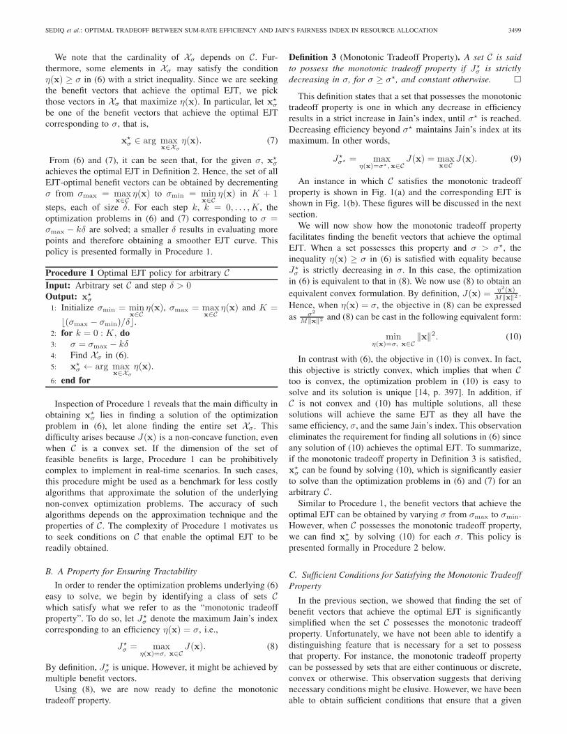
The comparisons between the optimal EJT and the tradeoffachieved by the α-fair policy for the case when the RBs can betime-shared among users are shown in Fig. 4(a) and Fig. 4(b).In Fig. 4(a), it is assumed that there is no minimum rateguarantee, i.e., xmin = 0, while in Fig. 4(b) the minimumrate guarantee is assumed to be xmin = 50 Kb/s. Procedure 2was used to obtain the optimal EJT, and the tradeoff achievedby the α-fair policy was obtained by solving (2). The convexoptimization problems underlying Procedure 2 and the α-fairpolicy were solved using ‘fmincon’, which is available inthe MATLAB optimization toolbox. From both figures, it canbe seen that, while these tradeoffs are close to each otherfor small and large values of α, for intermediate values, thetradeoff generated by the optimal EJT policy is significantlybetter than that generated by the α-fair one. For example, fora Jain’s index of 0.7, the optimal EJT policy provides 33%gain in efficiency as compared to the α-fair policy for the caseof xmin = 0 Kb/s and 21% gain in efficiency for the case ofxmin = 50 Kb/s.

In Figs. 5(a) and 5(b) we present the counterparts of


1 1.5 2 2.5 3 3.50.35

0.4

0.45

0.5

0.55

0.6

0.65

0.7

0.75

0.8

0.85

α increases

Jain

’sIn

dex


α = 70

α = 1

α = 0

Δη = 37%

ΔJ = 20%

α-fair Based Tradeoff

Optimal EJT (Proc. 1)

(a) xmin = 0 Kb/s.

1.4 1.6 1.8 2 2.2 2.4 2.60.55

0.6

0.65

0.7

0.75

0.8

0.85

0.9

α increases

Jain

’sIn

dex


α = 70

α = 1 α = 0

Δη = 37%

ΔJ = 4%


(b) xmin = 50 Kb/s.

Fig. 5. A comparison between the EJTs achieved by optimal and α-fairpolicies without time-sharing.

Figs. 4(a) and 4(b), but for the case when the RBs are nottime-shared by the users; in Fig. 5(a), xmin = 0, while inFig. 5(b) xmin = 50 Kb/s. Since the set C in this case is notconvex and hence does not satisfy the sufficient conditionsfor possessing the monotonic tradeoff property, Procedure 1was used to obtain the optimal EJT; cf. Section V-A. The non-convex optimization problems underlying Procedure 1 and theα-fair policy were solved using exhaustive search. Similar tothe case of time-sharing considered in Figs. 4(a) and 4(b),it can be seen from Figs. 5(a) and 5(b) that, in this case too,the optimal EJT policy provides tradeoffs that are significantlybetter than those provided by the α-fair policy when xmin = 0and when xmin = 50 Kb/s.

B. Case 2: Ergodic Time-Varying Channels

We now compare the performance of the α-fair schedulerin (18) with the one proposed in (20). To do so, we considera cellular network based on the IMT-Advanced guidelinesfor the Urban Macro (UMa) scenario [23]. As per theseguidelines, the number of hexagonal sectors is set to be57, which are served by 19 BSs. Each of these BSs hasa tri-sector antenna to serve a 3-sector cell-site. The users

TABLE ISIMULATION PARAMETERS BASED ON IMT-ADVANCED UMA SCENARIO.

Parameter Assumption or Value

Number of sectors 57Number of users 570Inter-site distance 500 m

BS height 25 mMin. distance b/w user and BS 25 m

User speed 30 km/hBandwidth (downlink) 10 MHz

Sub-carrier spacing 15 KHzNumber of RBs (N ) 50

OFDM symbol duration 66.67 µsNumber of sub-carriers per RB 12

Number of OFDM symbols per RB 7Carrier Frequency (GHz) 2.0Total BS transmit power 46 dBm

Number of drops 10Number of time slots per drop 10000

Smoothing factor (μ) 0.01BS antenna gain (boresight) 17 dBi

User antenna gain 0 dBiFeeder loss 2 dB

Channel estimation delay 4 time slotsSINR estimation margin 6 dB

Antenna tilt 12◦ [25, p. 4]Traffic model Full buffer

are uniformly dropped in the 57 sectors, and Monte Carlosimulations are carried over 104 time slots and averaged over10 independent drops. Users are assumed to be associated withthe sector with the highest received average power. This powerdepends on large channel variations, which are mainly due tonon-uniform antenna patterns (cf. [23, pp. 17–18]), distance-dependent path-loss and correlated shadowing. To incorporatethese variations in our simulations, we considered the line-of-sight (LOS) and non-line of-sight (NLOS) users as in [23,pp. 17–33]. For the LOS users, the path-loss exponent is setto be 2.2 and the shadowing is assumed log-normal withstandard deviation of 4 dB. For the NLOS users, the path-loss exponent is set to be 3.9 and the log-normal shadowingstandard deviation is set to be 6 dB. The system parametersare based on the LTE standard, whereby each RB is composedof a time slot of 7 OFDM symbols and 12 subcarriers [22].The simulation parameters are given in Table I.

In addition to large variations, the received signal power issubject to small-scale variations due to time-varying multipathfading. Variations of the received signal power due to fadingwithin each RB is negligible and hence, the channels can beassumed fixed over each RB. For other RBs the channels takeon different values depending on the spectro-temporal corre-lation of the IMT-Advanced model for the UMa scenario [24].

At time slot t, each user m ∈ M calculates its receivedsignal-to-interference-plus-noise ratios (SINRs) on all RBs,and subsequently determines rmn(t), the data rate that canbe reliably communicated on every RB n ∈ N . The set of allrates at time slot t, {rmn(t)}, are available at the BS, whichsubsequently determines the appropriate scheduling variables,{ρmn(t)}, depending on previously scheduled rates and theadopted scheduling strategy.

1) EJT Comparison: Using the UMa model with the aboveparameter settings, in Fig. 6 we plot the EJT curve for boththe α-fair scheduler in (18) and the optimal EJT scheduler


2 4 6 8 10 12 14 160.2

0.3

0.4

0.5

0.6

0.7

0.8

0.9

1

3 4 5 6 70.9

1Zoomed

Δη = 35%

α-fair Based SchedulingOptimal EJT Scheduling

Jain

’sIn

dex


Fig. 6. A long-term average rates comparison between the EJTs achievedby optimal and α-fair policies.

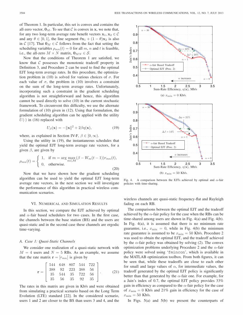
proposed in (20). From this figure it can be seen that thescheduler in (20) achieves a better tradeoff, especially inthe high fairness region. For example, for a Jain’s index of0.94, the scheduler in (20) provides 35% gain in efficiency ascompared to the α-fair scheduler.

2) User Satisfaction Comparison: To illustrate the advan-tage of using Jain’s index, we compare the number of satisfiedusers when the scheduling is performed based on the optimalEJT and α-fair policies. In particular, we assume that a useris satisfied if its long-term average rate exceeds a certainthreshold. To perform this comparison, for the α-fair policy,the parameter α is chosen to maximize the percentage of usersfor which the rates obtained by the scheduler in (18) exceeda given threshold. Similarly, for the proposed optimal EJTpolicy, the parameter β is chosen to maximize the percentageof users for which the rates obtained by the scheduler in (20)exceed the same threshold. Unfortunately, obtaining closed-form expressions for the optimal α and β as functions ofrate thresholds has proved intractable. As an alternative, foreach threshold we performed an exhaustive search to find theoptimal α and β that maximize the number of satisfied users ineach policy. In practice, the optimal α and β can be determinedthrough a pre-communication learning phase that enables theBSs to evaluate user satisfactions for tentative values of α andβ.

The comparison between the percentage of satisfied users atgiven rate thresholds is plotted in Fig. 7. As can be expected,the number of satisfied users is monotonically decreasing withthe threshold for both schedulers. However, the schedulerbased on the optimal EJT is consistently better than the onebased on the α-fair policy as it enables significantly moreusers to be satisfied. For instance, for the considered scenariowhen the threshold is set to be 1 Mb/s, the scheduler based onthe optimal EJT satisfies 10% more users than those satisfiedby the scheduler based on the α-fair policy. Hence, froma service provider’s perspective, using the scheduler basedon the optimal EJT yields a valuable increase in the abilityof the system to satisfy users with long-term average raterequirements.

0 0.5 1 1.5 2 2.5 310

20

30

40

50

60

70

80

90

100

α-fair Based SchedulingOptimal EJT Scheduling

Threshold (Mb/s)

Perc

enta

geof

Satis

fied

Use

rs(%

)

Fig. 7. Percentage of satisfied users for different thresholds.

VII. CONCLUSIONS

In this paper, we considered multiuser resource allocationsthat achieve the optimal tradeoff between efficiency and fair-ness from the Jain’s index perspective. We showed that, ingeneral, the commonly-used α-fair policy does not yield theoptimal EJTs except for the two-user case. To achieve the op-timal EJTs in the general case, we developed two procedures.In the first procedure, the set of feasible allocations is arbitrary,but finding the allocations that achieve the optimal EJTsinvolves solving potentially difficult optimization problems.In contrast, in the second procedure, the set of feasibleallocations is assumed to have a monotonic property that arisesin many practical scenarios. This property is exploited tofacilitate the search for allocations that achieve the optimalEJTs, and is shown to arise naturally in the problem ofscheduling radio resources in quasi-static and ergodic time-varying communication scenarios. This property enables usto devise computationally-efficient schedulers that achievethe optimal EJT. Our analysis is supported by illustrations,geometric interpretations and numerical examples.

ACKNOWLEDGMENT

The authors would like to express their gratitude to Dr.Gamini Senarath, Dr. Ho Ting Cheng, and Dr. Petar Djukicof Huawei Technologies Canada Co., Ltd.

APPENDIX APROOF OF PROPOSITION 1

We will proceed by contradiction. Let α ∈ (0,∞) be givenand suppose that x�

α does not achieve the optimal EJT, that is,there exists a non α-fair optimal vector x such that either: 1)η(x) > η (x�

α) and J(x) ≥ J (x�α); or 2) η(x) ≥ η (x�

α) andJ(x) > J (x�

α). We will show that such a vector x results inUα(x) > Uα(x

�α), which contradicts the definition of α-fair

benefit vectors; cf. (2). We will focus on the first case. Theproof for the second case follows similar lines and is omittedfor brevity.

Since M = 2, we can define a parameter ω = maxxminx . Using

this ω, we have J(x) = (1+ω)2

2(1+ω2) . Now, dJdω = − ω2−1

(ω2+1)2 . Since,


by definition, ω ≥ 1, it can be seen that J is monotonicallydecreasing in ω. This with the fact that, in the considered case,J(x) ≥ J (x�

α) implies that

maxx

minx≤ maxx�

α

minx�α

. (22)

Since in this case we also have η(x) > η(x�α), it follows that

minx + maxx > minx�α + maxx�

α, which is equivalent to(1 + maxx

minx

)minx >

(1 +

maxx�α

minx�α

)minx�

α. This inequalityimplies that

minx >

(1 +

maxx�α

minx�α

)(1 + maxx

minx

) minx�α. (23)

Invoking (22) implies that the fraction on the right hand sideis greater than 1, which further implies that we can writeminx = minx�

α + ε1, with ε1 > 0. Since x is not α-fair,we must have

Uα(x) < Uα(x�α). (24)

We now observe that Uα(x) is strictly increasing in each xm,m = 1, 2. This observation and (24) imply that maxx =maxx�

α − ε2, with ε2 > 0. Combining this with the fact thatminx = minx�

α + ε1 and the fact that in the current caseη(x) > η (x�

α) yields ε1 > ε2. Using this notation, it can bereadily verified that, because ε1 > ε2,

∇Uα(x)T (x�

α − x) = −ε1(minx)−α(1− ε2

ε1

(maxxminx

)−α)

< 0,

Now, direct computation of the Hessian of Uα(x) showsthat Uα is concave for any α ∈ (0,∞). Thus [14, p. 69],Uα(x

�α) ≤ Uα(x) +∇Uα(x)

T (x�α − x), which yields

Uα(x�α) < Uα(x). (25)

This with (24) establish the desired contradiction.

APPENDIX BPROOF OF THEOREM 1

Let x�σ1

and x�σ2

be the benefit vectors obtained using (10)with σ1 and σ2, respectively, where σmin ≤ σ1 < σ2 ≤ σmax.To prove Theorem 1, it suffices to show that if the conditionsof the theorem are satisfied, then J�

σ1≥ J�

σ2with equality if

and only if J�σ2

= J�σ� , where J�

σ and J�σ� are given by (8)

and (9), respectively. We consider two distinct cases: xmin > 0and xmin = 0.

Case 1 (xmin > 0): First we note that, because xmin1 ∈C, J�

σ� = 1. Now, the convexity of C implies that, for anyθ ∈ (0, 1),

yθ = θxmin1+ (1− θ)x�σ2∈ C. (26)

Substituting for yθ from (26) in (1), it can be verified that

J(yθ)− J�σ2

= a(1− J(yθ)), (27)

where a =θ2M2x2

min+2θ(1−θ)Mxmin1Tx�

σ

M(1−θ)2x�σTx�

σ≥ 0.

To prove the theorem, we will show that J(yθ)− J�σ2≥ 0,

with equality if and only if J�σ2

= 1. To do so, we note that,by the properties of Jain’s index, if J�

σ2< 1, then x�

σ2= γ11,

and subsequently from (26) yθ = γ21 for any γ1, γ2 > 0. This

implies that J(yθ) < 1. This with (27) and the fact that a > 0for any θ ∈ (0, 1) further implies that J(yθ) > J�

σ2. We next

show that there exists a θ0 ∈ (0, 1) such that η(yθ0) = σ1. Inparticular, setting θ0 = σ2−σ1

σ2−Mxminyields this efficiency. Since

J�σ1

is the maximum Jain’s index corresponding to η(x) = σ1,we must have J�

σ1≥ J(yθ0), which implies that J�

σ1> J�

σ2.

For the case of J�σ2

= 1, we note that yθ = γ21, for some γ2and therefore, by the homogeneity of Jain’s index, J(yθ) = 1for any θ. The statement of the theorem follows by using anargument analogous to the above and noting that J�

σ ≤ 1, forany σ including σ1.

Case 2 (xmin = 0): The proof for the case of xmin > 0does not hold when xmin = 0. Furthermore, it is easy to findsets C for which xmin = 0, but vectors of the form γ11 /∈ Ceven for infinitesimal values of γ1 > 0, e.g., C = {x1, x2 :0 ≤ x2 ≤ cx1}, where c ∈ (0, 1).

To prove the theorem for this case, we provide the followinglemma:

Lemma 1. Let C be a set satisfying the conditions of Theo-rem 1 with xmin = 0 and let σmin ≤ σ1 ≤ σ2 ≤ σmax, thenJ�σ1≥ J�

σ2.

Before providing the proof, we note that, unlike the claim ofTheorem 1, this lemma does not tell whether a strict decreasein σ will yield a strict increase in Jain’s index.

Proof: Let x�σ2

be the optimal benefit vector at efficiencyσ2; that is, J(x�

σ2) = J�

σ2. Since C is convex and 0M ∈ C, it

follows that, for any θ ∈ [0, 1], x = θx�σ2∈ C. Noting that

σ1 ≤ σ2 and setting θ = σ1

σ2, it can be seen that η(x) = σ1.

Now, the homogeneity of Jain’s index implies that J(x) =J�σ2

. However, J�σ1

is the optimal Jain’s index at efficiencyσ1 and hence J�

σ1≥ J(x), which completes the proof of the

lemma.We now proceed to complete the proof of Theorem 1. Let

σ� be the highest efficiency corresponding to the maximumachievable Jain’s index, i.e., J�

σ� . We will consider two cases:σ2 ≤ σ� and σ2 > σ�.

When σ2 ≤ σ�, we have by assumption that σ1 < σ�,which, by Lemma 1, implies that J�

σ2= J�

σ1= J�

σ2, and the

theorem is proved in this case.We now consider the case of σ2 > σ�. We again consider

two cases: σ1 ≤ σ� and σ1 > σ�.Since σ2 > σ�, it follows by the definition of σ� that J�

σ2<

J�σ� . Now, if σ1 ≤ σ�, invoking Lemma 1 yields J�

σ1= J�

σ� ,which implies that J�

σ2< J�

σ1.

We next prove the theorem for the remaining case of σ2 >σ1 > σ�.

For this case, we will consider the line segment, yθ ,connecting x�

σ2with x�

σ�, i.e., yθ = θx�

σ�+ (1 − θ)x�

σ2,

θ ∈ [0, 1]. The convexity assumption implies that yθ ∈ C.Substituting for yθ in (1), it can be verified that, for any x�

σ2

and yθ such that ‖x�σ2‖‖yθ‖ > 0,

J(yθ)− J(x�σ2) =

θ2(σ�2‖x�σ2

‖2−σ22‖x�

σ�‖2)+2θ(1−θ)σ2(σ

�‖x�σ2

‖2−σ2x�σ�

Tx�σ2

)

M‖x�σ2

‖2‖yθ‖2 .

(28)We will now use this equality to show that J(yθ) > J(x�

σ2).

For the first term in the numerator, we note that, since byassumption σ2 > σ�, we have J�

σ2< J�

σ� . This implies that


σ�2‖x�σ2‖2 − σ2

2‖x�σ�‖2 > 0. For the second term, we note

that, by the Cauchy-Schwartz inequality,

σ�‖x�σ2‖2 − σ2x

�σ�

Tx�σ2≥ ‖x�

σ2‖(σ�‖x�

σ2‖ − σ2‖x�

σ�‖) > 0.

The strict positivity follows from the fact that J�σ2

< J�σ� .

Hence, we have shown that J(yθ) > J(x�σ2) for any θ ∈

(0, 1).We next show that there exists a θ0 ∈ (0, 1) such that

η(yθ0) = σ1. In particular, setting θ0 = σ2−σ1

σ2−σ� yields thisefficiency, where θ0 ∈ (0, 1) by the assumption that σ1 > σ�.Since J�

σ1is the maximum Jain’s index corresponding to

η(x) = σ1, we must have J�σ1≥ J(yθ0), which implies that

J�σ1

> J�σ2

and completes the proof of the theorem.

REFERENCES

[1] J. Mo and J. Walrand, “Fair end-to-end window-based congestioncontrol,” IEEE/ACM Trans. Netw., vol. 8, no. 5, pp. 556–567, Oct. 2000.

[2] T. Lan, D. Kao, M. Chiang, and A. Sabharwal, “An axiomatic theory offairness in network resource allocation,” in Proc. 2010 IEEE Int. Conf.Comput. Commun.

[3] H. T. Cheng and W. Zhuang, “An optimization framework for balancingthroughput and fairness in wireless networks with QoS support,” IEEETrans. Wireless Commun., vol. 7, no. 2, pp. 584–593, Feb. 2008.

[4] R. Schoenen, A. Bin Sediq, H. Yanikomeroglu, G. Senarath, andZ. Chao, “Fairness analysis in cellular networks using stochastic Petrinets,” in Proc. 2011 IEEE Int. Symp. Pers., Indoor Mobile RadioCommun.

[5] R. Schoenen, A. Bin Sediq, H. Yanikomeroglu, G. Senarath, Z. Chao,and H. T. Cheng, “Spectral efficiency and fairness tradeoffs in cellularnetworks with realtime+nonrealtime traffic mix using stochastic Petrinets,” in Proc. 2012 IEEE Veh. Tech. Conf. – Fall.

[6] D. Bertsekas and R. Gallager, Data Networks, 2nd ed. Prentice Hall,1992.

[7] A. Odlyzko, “Network neutrality, search neutrality, and the never-ending conflict between efficiency and fairness in markets,” Rev. Netw.Economics, vol. 8, no. 1, pp. 40–60, Mar. 2009.

[8] M. Zukerman, L. Tan, H. Wang, and I. Ouveysi, “Efficiency-fairnesstradeoff in telecommunications networks,” IEEE Commun. Lett., vol. 9,no. 7, pp. 643–645, July 2005.

[9] R. Jain, D. Chiu, and W. Hawe, “A quantitative measure of fairnessand discrimination for resource allocation in shared systems,” DigitalEquipment Corporation, DEC-TR-301, Tech. Rep., 1984. Available:http://www1.cse.wustl.edu/∼jain/papers/ftp/fairness.pdf.

[10] F. P. Kelly, A. K. Maulloo, and D. K. H. Tan, “Rate control for commu-nication networks: shadow prices, proportional fairness and stability,” J.Oper. Res. Soc., vol. 49, no. 3, pp. 237–252, 1998.

[11] C. Wengerter, J. Ohlhorst, and A. von Elbwart, “Fairness and through-put analysis for generalized proportional fair frequency scheduling inOFDMA,” in Proc. 2005 IEEE Veh. Tech. Conf. – Spring.

[12] C. Joe-Wong, S. Sen, T. Lan, and M. Chiang, “Multi-resource allocation:Fairness-efficiency tradeoffs in a unifying framework,” in Proc. 2012IEEE Int. Conf. Comput. Commun.

[13] A. Ibing and H. Boche, “Fairness vs. efficiency: comparison of gametheoretic criteria for OFDMA scheduling.” in Proc. 2007 Asilomar Conf.Signals, Syst., Comput.

[14] S. Boyd and L. Vandenberghe, Convex Optimization. Cambridge Uni-versity Press, 2004.

[15] A. Bin Sediq, R. H. Gohary, and H. Yanikomeroglu, “Optimal tradeoffbetween efficiency and Jain’s fairness index in resource allocation,” inProc. 2012 IEEE Int. Symp. Pers., Indoor Mobile Radio Commun.

[16] B. Radunovic and J.-Y. L. Boudec, “Rate performance objectives ofmultihop wireless networks,” IEEE Trans. Mobile Comput., vol. 3, no. 4,pp. 334–349, Oct. 2004.

[17] G. Song and Y. Li, “Cross-layer optimization for OFDM wirelessnetworks—part II: algorithm development,” IEEE Trans. Wireless Com-mun., vol. 4, no. 2, pp. 625–634, Mar. 2005.

[18] E. Biglieri, J. Proakis, and S. Shamai (Shitz), “Fading channels:information-theoretic and communication aspects,” IEEE Trans. Inf.Theory, vol. 44, no. 6, pp. 2619–2692, Oct. 1998.

[19] C. Y. Wong, R. S. Cheng, K. Ben Letaief, and R. D. Murch, “MultiuserOFDM with adaptive subcarrier, bit, and power allocation,” IEEE J. Sel.Areas Commun., vol. 17, no. 10, pp. 1747–1758, Oct. 1999.

[20] A. L. Stolyar, “On the asymptotic optimality of the gradient schedulingalgorithm for multiuser throughput allocation,” Oper. Res., vol. 53, no. 1,pp. 12–25, Jan. 2005.

[21] H. Kushner and P. Whiting, “Convergence of proportional-fair sharingalgorithms under general conditions,” IEEE Trans. Wireless Commun.,vol. 3, no. 4, pp. 1250–1259, July 2004.

[22] E. Dahlman, S. Parkvall, J. Skold, and P. Beming, 3G Evolution: HSPAand LTE for Mobile Broadband, 2nd ed. Academic Press, 2008.

[23] ITU, Report ITU-R M.2135-1, “Guidelines for evaluation of radiointerface technologies for IMT-Advanced,” ITU, Tech. Rep., Dec. 2009.Available: http://www.itu.int/pub/R-REP-M.2135-1-2009.

[24] J. Nystrom, “Software implementation of IMT.Eval channel model,”CELTIC/CP5-026 Project WINNER+ Doc. 5D/478-E, Tech. Rep., July2009. Available: http://www.itu.int/oth/R0A06000022/en.

[25] “Calibration for IMT-Advanced evaluations,” CELTIC/CP5-026Project WINNER+, Tech. Rep., May 2010. Available: http://projects.celtic-initiative.org/winner+/WINNER+EvaluationGroup.html.

Akram Bin Sediq (S’04) received the B. Sc. degreein Electrical Engineering (summa cum laude) in2006 from the American University of Sharjah,United Arab Emirates, and the M.A.Sc. degreein Electrical Engineering in 2008 from CarletonUniversity, Ottawa, Canada, where he is currentlyworking towards the Ph.D. degree in wireless com-munications. In Winter 2012, Mr. Bin Sediq was acourse instructor at the Department of Systems andComputer Engineering at Carleton University.

He has been conducting research in collaborationwith Huawei Technologies, which resulted in three patent applications. Hisresearch interests include inter-cell interference coordination, radio resourceallocations, heterogenous networks, constellation design, cooperative commu-nications, and applications of optimization in wireless networks.

Mr. Bin Sediq is a recipient of the IEEE Antennas and PropagationSociety Undergraduate Scholarship in 2004, the IEEE Microwave Theoryand Techniques Society Undergraduate/Pre-Graduate Scholarship in 2005,the third prize in IEEE IAS Myron Zucker Undergraduate Student DesignContest in 2005, the President Cup for graduating with the highest GPA at theBachelor’s level in 2006, the Ontario Graduate Scholarship for internationalstudents for three years in a row during 2007–2010, the Senate Medal foroutstanding academic achievement from Carleton University at the Master’slevel in 2008, and the EDC Teaching Assistant Outstanding Award at CarletonUniversity in 2013.

Ramy H. Gohary (S’02-M’06-SM’13) received theB.Sc. (Hons.) degree from Assiut University, Egyptin 1996, the M.Sc. degree from Cairo University,Egypt, in 2000, and the Ph.D. degree from Mc-Master University, Ontario, Canada in 2006, allin electronics and communications engineering. Hereceived the Natural Sciences and Engineering Re-search Council visiting fellowship award in 2007.

Dr. Gohary was a visiting scientist with the Ter-restrial Wireless Systems Branch, CommunicationsResearch Centre, Canada. He is currently the project

manager of the Carleton-BlackBerry (formerly Research In Motion (RIM))research project.

His research interests include analysis and design of MIMO wirelesscommunication systems, applications of optimization and geometry in signalprocessing and communications, information theoretic aspects of multiusercommunication systems, and applications of iterative detection and decodingtechniques in multiple antenna and multiuser systems.


Rainer Schoenen received his German Diplom-Ingenieur and Ph.D. degrees from RWTH AachenUniversity, in Electrical Engineering in 1995 and2000, respectively. His research interests includestochastic Petri nets and queuing systems, ATM,TCP/IP, switching, flow control, QoS, tariffs, User-in-the-loop (UIL), wireless resource and packetscheduling and the MAC layer of 4+5G systems. HisPh.D. thesis was “System Components for Broad-band Universal Networks with QoS Guarantee.” withthe ISS group of Prof. Heinrich Meyr at RWTH

Aachen University, Germany, from 1995 to 2000. He started working self-employed in 2000. Dr. Schoenen was a senior researcher at the Communi-cation Networks (ComNets) Research Group, RWTH Aachen with ProfessorWalke from 2005 to 2009, working on computer networks, queuing theory,Petri nets, LTE-Advanced, FDD relaying, scheduling, OSI layer 2 (MAC)and IMT-Advanced Evaluation within WINNER+. He is currently a projectmanager at the Department of Systems and Computer Engineering, CarletonUniversity, Ottawa, Canada, working with Professor Halim Yanikomeroglu.

Halim Yanikomeroglu (S’96–M’98–SM’12) wasborn in Giresun, Turkey, in 1968. He received theB.Sc. degree in Electrical and Electronics Engi-neering from the Middle East Technical University,Ankara, Turkey, in 1990, and the M.A.Sc. degreein Electrical Engineering (now ECE) and the Ph.D.degree in Electrical and Computer Engineering fromthe University of Toronto, Canada, in 1992 and1998, respectively. He was with the R&D Groupof Marconi Kominikasyon A.S., Ankara, Turkey,during 1993–1994.

Since 1998 Dr. Yanikomeroglu has been with the Department of Sys-tems and Computer Engineering at Carleton University, Ottawa, wherehe is now a Full Professor. His research interests cover many aspectsof wireless technologies with special emphasis on cellular networks. Dr.Yanikomeroglu coauthored more than 50 journal and 160 conference papers,and has given more than 20 tutorials in leading international conferenceson wireless technologies. In recent years, Dr. Yanikomeroglu’s research hasbeen funded by Huawei, BlackBerry (formerly Research in Motion (RIM)),Samsung, Communications Research Centre (CRC) of Canada, Telus, andNortel. This collaborative research resulted in about 15 patent applications.Dr. Yanikomeroglu is a member of the Steering Committee of the IEEEWireless Communications and Networking Conference (WCNC), and hasbeen involved in the organization of this conference over the years, includingserving as the Technical Program Co-Chair of WCNC 2004 and the TechnicalProgram Chair of WCNC 2008; he will also serve as the Technical ProgramCo-Chair of WCNC 2014 to be held in Istanbul. Dr. Yanikomeroglu wasthe General Co-Chair of the IEEE Vehicular Technology Conference Fall2010 held in Ottawa. Dr. Yanikomeroglu has served in the editorial boards ofthe IEEE TRANSACTIONS ON COMMUNICATIONS, IEEE TRANSACTIONS

ON WIRELESS COMMUNICATIONS, and IEEE COMMUNICATIONS SURVEYS

& TUTORIALS. He was the Chair of the IEEE’s Technical Committee onPersonal Communications (now called, Wireless Technical Committee). Heis a Distinguished Lecturer for the IEEE Vehicular Technology Society.

Dr. Yanikomeroglu is a recipient of the Carleton University Faculty Grad-uate Mentoring Award in 2010, the Carleton University Graduate StudentsAssociation Excellence Award in Graduate Teaching in 2010, and the CarletonUniversity Research Achievement Award in 2009. Dr. Yanikomeroglu spentthe 2011–2012 academic year at TOBB University of Economics and Tech-nology, Ankara, Turkey, as a Visiting Professor. He is a registered ProfessionalEngineer in the province of Ontario, Canada.

3496 ieee transactions on wireless ......3496 ieee transactions on wireless communications, vol. 12,...

Documents