13.021 – Marine Hydrodynamics, Fall 2004Lecture 10

Copyright c© 2004 MIT - Department of Ocean Engineering, All rights reserved.

13.021 - Marine HydrodynamicsLecture 10

3.5 - Boundary Conditions for Potential Flow

Types of Boundary Conditions:

1. Kinematic Boundary Conditions - specify the flow velocity ~v at boundaries.

2. Dynamic Boundary Conditions - specify force ~F or pressure p at flow boundary.

• Kinematic Boundary Conditions on an impermeable boundary (no flux condition):

⇀n · ~v =

⇀n · ⇀

U = Un (given) where ~v = ∇φ⇀n · ∇φ = Un −→ ∂φ

∂n= Un

∂∂n

=(n1

∂∂x1

+ n2∂

∂x2+ n3

∂∂x3

)

( )321 n,n,nn =�

( )�

U�

• Dynamic Boundary Conditions: Pressure is prescribed in general.

p = −ρ

(φt +

1

2(∇φ)2 + gy

)+ C (t) (prescribed)

1

In general:

( )�

( ) giventCgy2

1 2

t��

�

�

��

�

�+��

�

�

�+φ∇+φρ−

↓

non-linear

Free surface

02 =φ∇

(�

givenn

=∂

φ∂

( )�

( ) giventCgy2

1 2

t��

�

�

��

�

�+��

�

�

�+φ∇+φρ−

↓

non-linear

Free surface

02 =φ∇

(�

givenn

=∂

φ∂

Linear Superposition for Potential Flow

In the absence of dynamic boundary conditions, the potential flow boundary value problem islinear.

• Potential function φ.

BonfUn n ==

∂φ∂

Vin02 =φ∇

• Stream function ψ.

2

Vin02 =ψ∇

ψ=g on B

Linear Superposition: if φ1, φ2, . . . are harmonic functions, i.e. ∇2φi = 0, then φ =∑

αiφi, whereαi are constants, are also harmonic, and is the solution for the boundary value problem provided theboundary conditions (kinematic boundary condition) are satisfied, i.e.

∂φ

∂n=

∂

∂n(α1φ1 + α2φ2 + . . .) = Un on B.

The key is to combine known solution of the Laplace equation in such a way as to satisfy the K.B.C.(kinematic boundary condition).The same is true for the stream function ψ. K.B.C.s specify the value of ψ on the boundaries.

Example:

φi

(⇀x)is a unit-source flow with source at

⇀xi

i.e.

φi

(⇀x) ≡ φsource

(⇀x,

⇀xi

)=

1

2πln

∣∣⇀x − ⇀

xi

∣∣ (in 2D)

= − (4π

∣∣⇀x − ⇀

xi

∣∣)−1(in 3D),

then find mi such that:

φ =∑

i

miφi(⇀x) satisfies KBC on B

Caution: φ must be regular for x ∈ V , so it is required that ~x /∈ V .

3

1x�

•

2x�•

4x�•

3x�•

Vin02 =φ∇

fn

=∂Φ∂

Figure 1: Note: ~xj, j = 1, . . . , 4 are not in the fluid domain V .

Laplace equation in different coordinate systems (cf Hildebrand §6.18)1. Cartesian (x,y,z)

~v =

(iu,

jv,

kw

)= ∇φ =

(∂φ

∂x,∂φ

∂y,∂φ

∂z

)

∇2φ =

(∂2φ

∂x2+

∂2φ

∂y2+

∂2φ

∂z2

)

z

x

(x,y,z)

y

2. Cylindrical (r,θ,z)

4

r2 = x2 + y2,

θ = tan−1(y/x)

⇀v =

(ervr,

eθvθ,

ezvz

)=

(∂φ

∂r,1

r

∂φ

∂θ,∂φ

∂z

)

∇2φ =

∂2φ

∂r2+

1

r

∂φ

∂r︸ ︷︷ ︸1r

∂φ∂r (r ∂φ

∂r )

+1

r2

∂2φ

∂θ2+

∂2φ

∂z2

y

z

x

r

θ

z

)z,r,(

3. Spherical (r,θ,ϕ)

r2 = x2 + y2 + z2,

θ = cos−1(x/r) or x = r (cos θ)

ϕ = tan−1(z/y)

⇀v = ∇φ =

(ervr,

eθvθ,

eϕ

vϕ

)=

(∂φ

∂r,1

r

∂φ

∂θ,

1

r(sin θ)

∂φ

∂ϕ

)

5

∇2φ =

∂2φ

∂r2+

2

r

∂φ

∂r︸ ︷︷ ︸1

r2∂∂r (r2 ∂φ

∂r )

+1

r2 sin θ

∂

∂θ

(sin θ

∂φ

∂θ

)+

1

r2 sin2 θ

∂2φ

∂ϕ2

z

x

y

r(sinθ)

ϕ θ

),(r, ϕθ

3.7 - Simple Potential flows

1. Uniform Stream: ∇2(ax + by + cz + d) = 0

1D: φ = Ux + constant ψ = Uy + constant⇀v = (U, 0, 0)

2D: φ = Ux + V y + constant ψ = Uy − V x + constant⇀v = (U, V, 0)

3D: φ = Ux + V y + Wz + constant⇀v = (U, V,W )

2. Source (sink) flow:

2D: Polar coordinates

∇2 =1

r

∂

∂r

(r

∂

∂r

)+

1

r2

∂2

∂θ2, with r =

√x2 + y2

An axisymmetric solution: φ = ln r (verify)

6

Define 2D source of strength m at r = 0:

φ =m

2πln r

It satisfies ∇2φ = 0, except at r =√

x2 + y2 = 0 (so must exclude r = 0 from flow)

∇φ =∂φ

∂rer =

m

2πrer, i.e. vr =

m

2πr, vθ = 0

source (strength m)

x

y

Net outward volume flux is

∮C

⇀v · nds =

∫∫S

∇ · ⇀vds =

∫∫Sε

∇ · ⇀vds

∮Cε

⇀v · nds =

2π∫0

Vr︸︷︷︸m

2πrε

rεdθ = m︸︷︷︸source

strength

7

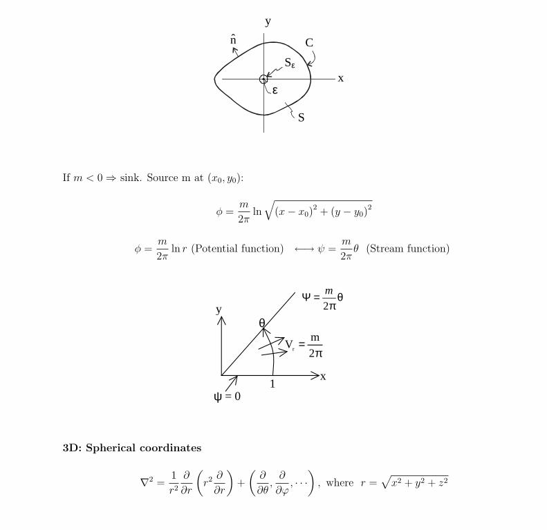
C

S

ε

Sε

n

x

y

If m < 0 ⇒ sink. Source m at (x0, y0):

φ =m

2πln

√(x− x0)

2 + (y − y0)2

φ =m

2πln r (Potential function) ←→ ψ =

m

2πθ (Stream function)

y

x

θ

ψ = 0 1

π=

2

mVr

θπ

=Ψ2

m

3D: Spherical coordinates

∇2 =1

r2

∂

∂r

(r2 ∂

∂r

)+

(∂

∂θ,

∂

∂ϕ, · · ·

), where r =

√x2 + y2 + z2

8

A spherically symmetric solution: φ = 1r

(verify ∇2φ = 0 except at r = 0)

Define 3D source of strength m at r = 0:

φ = − m

4πr, then Vr =

∂φ

∂r=

m

4πr2, Vθ, Vϕ = 0

Net outward volume flux is

∫∫©VrdS = 4πr2

ε ·m

4πr2ε

= m (m < 0 for a sink )

3. 2D point vortex

∇2 =1

r

∂

∂r

(r

∂

∂r

)+

1

r2

∂2

∂θ2

Another particular solution: φ = aθ + b (verify ∇2φ = 0 except at r = 0)

Define the potential for a point vortex of circulation Γ at r = 0:

φ =Γ

2πθ, then Vr =

∂φ

∂r= 0, Vθ =

1

r

∂φ

∂θ=

Γ

2πrand ωz =

1

r

∂

∂r(rVθ) = 0 except at r = 0

Stream function:

ψ = − Γ

2πln r

Circulation:

∫

C1

⇀v · d⇀

x =

∫

C2

⇀v · d⇀

x +

∫

C1−C2

⇀v · d⇀

x

︸ ︷︷ ︸∫ ∫S

ωzdS=0

=

2π∫

0

Γ

2πrrdθ = Γ︸︷︷︸

vortexstrength

9

C1

C2

S

0=zω

4. Dipole (doublet flow)

A Dipole is a superposition of a sink and a source with the same strength.

2D dipole:

10

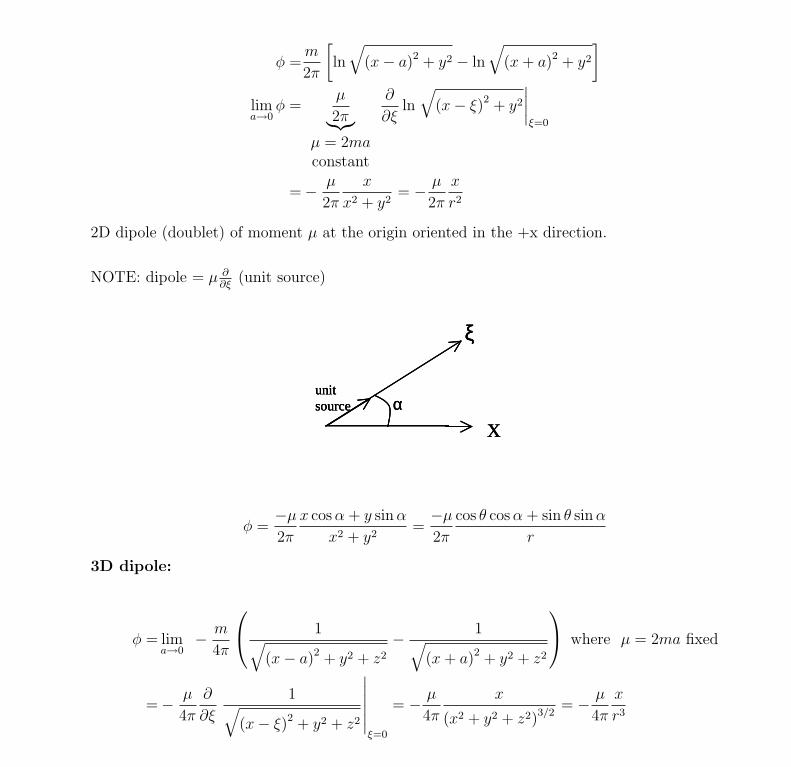
φ =m

2π

[ln

√(x− a)2 + y2 − ln

√(x + a)2 + y2

]

lima→0

φ =µ

2π︸︷︷︸µ = 2maconstant

∂

∂ξln

√(x− ξ)2 + y2

∣∣∣∣ξ=0

=− µ

2π

x

x2 + y2= − µ

2π

x

r2

2D dipole (doublet) of moment µ at the origin oriented in the +x direction.

NOTE: dipole = µ ∂∂ξ

(unit source)

ξ

α unit source

x

ξ

α unit source

ξ

α unit source

x

φ =−µ

2π

x cos α + y sin α

x2 + y2=−µ

2π

cos θ cos α + sin θ sin α

r

3D dipole:

φ = lima→0

− m

4π

1√

(x− a)2 + y2 + z2

− 1√(x + a)2 + y2 + z2

where µ = 2ma fixed

=− µ

4π

∂

∂ξ

1√(x− ξ)2 + y2 + z2

∣∣∣∣∣∣ξ=0

= − µ

4π

x

(x2 + y2 + z2)3/2= − µ

4π

x

r3

11

3D dipole (doublet) of moment µ at the origin oriented in the +x direction.

5. Stream and source: Rankine half-body

It is the superposition of a uniform stream of constant speed U and a source of strengthm.

U

m

2D:

φ = Ux +m

2πln

√x2 + y2

DU

U

x m

stagnation point 0v =�

Dividing Streamline

u = ∂φ∂x

= U + m2π

xx2+y2

u|y=0 = U + m2πx

∴ u = 0 at x = xs = − m2πU

12

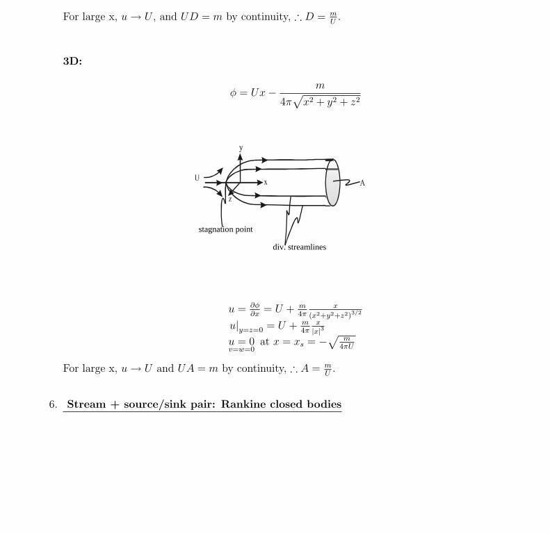
For large x, u → U , and UD = m by continuity, ∴ D = mU

.

3D:

φ = Ux− m

4π√

x2 + y2 + z2

div. streamlines

stagnation point

u = ∂φ∂x

= U + m4π

x

(x2+y2+z2)3/2

u|y=z=0 = U + m4π

x|x|3

u = 0v=w=0

at x = xs = −√m

4πU

For large x, u → U and UA = m by continuity, ∴ A = mU

.

6. Stream + source/sink pair: Rankine closed bodies

13

U SS x

y

+m -m

a

dividing streamline (see this with PFLOW)

To have a closed body, a necessary condition is to have∑

min body = 0

2D Rankine ovoid:

φ = Ux +m

2π

(`n

√(x + a)2 + y2 − `n

√(x− a)2 + y2

)

3D Rankine ovoid:

φ = Ux− m

4π

1√

(x + a)2 + y2 + z2

− 1√(x− a)2 + y2 + z2

For Rankine Ovoid,

u =∂φ

∂x= U +

m

4π

[x + a

((x + a)2 + y2 + z2

)3/2− x− a

((x− a)2 + y2 + z2

)3/2

]

u|y=z=0 =U +m

4π

[1

(x + a)2 −1

(x− a)2

]

=U +m

4π

(−4ax)

(x2 − a2)2

u|y=z=0 =0 at(x2 − a2

)2=

( m

4πU

)4ax

14

At x = 0,

u = U +m

4π

2a

(a2 + R2)3/2where R = y2 + z2

Determine radius of body R0:

2π

R0∫

0

uRdR = m

7. Stream + Dipole: circles and spheres

U µ

r

θ

2D:

φ =Ux +µx

2πr2, where x = r cos θ

= cos θ(Ur +

µ

2πr

)then Vr =

∂φ

∂r= cos θ

(U − µ

2πr2

)

So Vr = 0 on r = a =√

µ2πU

}(which is the K.B.C. for a stationary circle radius a) or choose

µ = 2πUa2.

Steady flow past a circle (U,a):

15

φ = U cos θ(r + a2

r

)

Vθ = 1r

∂φ∂θ

= −U sin θ(1 + a2

r2

)

Vθ|r=a = −2U sin θ

{= 0 at θ = 0, π SA and SB − stagnation points.= ∓2U at θ = π

2, 3π

2maximum tangential velocity

2U

2U

θ

Illustration of the points where the flow reaches maximum speed around the circle.

3D:

16

y

x

r

z

U

µ

θ

φ = Ux + µ4π

cos θr2 , x = r cos θ

Vr = ∂φ∂r

= cos θ(U − µ

2πr3

)Vr = 0 on r = a︸ ︷︷ ︸

K.B.C. onstationarysphere ofradius a

→ a = 3√

µ2πU

or µ = 2πUa3

Steady flow past a sphere (U, a):

φ = U cos θ(r + a3

2r2

)

Vθ = 1r

∂φ∂θ

= −U sin θ(1 + a3

2r3

)

Vθ |r=a = −3U2

sin θ

{= 0 at θ = 0, π= −3U

2at θ = π

2

x

2

3U

θ

17

8. 2D corner flow

Potential function: φ = rα cos αθ, and the Stream function: ψ = rα sin αθ

(a) ∇2φ =(

∂2

∂r2 + 1r

∂∂r

+ 1r2

∂2

∂θ2

)φ = 0

(b)ur = ∂φ

∂r= αrα−1 cos αθ

uθ = 1r

∂φ∂θ

= −αrα−1 sin αθ∴ uθ = 0 { or ψ = 0} on αθ = nπ, n = 0,±1,±2, . . .

i.e. on θ = θ0 = 0, πα, 2π

α, . . . (θ0 ≤ 2π)

i. interior corner flow – stagnation point origin: α > 1.

e.g. α = 1, θ0 = 0, π, 2π, u = 1, v = 0

x

y

ψ = 0

18

(90o corner)

ψ = 0

ψ = 0

y2v,x2u2,2

3,,

2,0,2 0 −==ππππ=θ=α

(120o corner)

θ=0, ψ = 0

θ=2π/3, ψ = 0

θ=2π, ψ = 0

θ=4π/3, ψ = 0

120o

120o

120o πππ=θ=α 2,3

4,

3

2,0,23 0

19

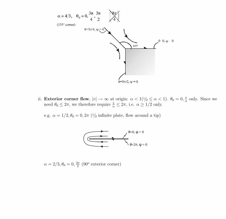
ii. Exterior corner flow, |v| → ∞ at origin: α < 1(1/2 ≤ α < 1). θ0 = 0, πα

only. Since weneed θ0 ≤ 2π, we therefore require π

α≤ 2π, i.e. α ≥ 1/2 only.

e.g. α = 1/2, θ0 = 0, 2π (1/2 infinite plate, flow around a tip)

θ=0, ψ = 0

θ=2π, ψ = 0

α = 2/3, θ0 = 0, 3π2

(90o exterior corner)

20

θ=3π/2, ψ = 0

θ=0, ψ = 0

21