3b.1 an extension of the advancing front method to ...imr.sandia.gov/papers/imr16/foucault.pdf ·...

3B.1An Extension of the Advancing Front Method to Composite Geometry

G. Foucault(1), J-C. Cuillière(1), V. François(1), J-C. Léon(2), R. Maranzana(3)

(1) Université du Québec à Trois-Rivières, CP 500, Trois-Rivières (Québec) G9A-5H7, Canada Gilles.Foucault, Jean-Christophe.Cuilliere, Vincent.Francois @uqtr.ca(2) Institut National Polytechnique de Grenoble, Laboratoire G-SCOP, France, [email protected] (3) Ecole de Technologie Supérieure de Montréal, GPA, Laboratoire LIPPS, Canada, [email protected]

AbstractThis paper introduces a new approach to automatic mesh generation over

composite geometry. This approach is based on an adaptation of advancing front mesh generation techniques over curved surfaces, and its main features are :

elements are generated directly over multiple parametric surfaces: advancing front propagation is adapted through the extension to composite geometry of propagation direction, propagation length, and target point concepts, each mesh entity is associated with sets of images in each reference entity of the composite geometry, the intersection tests between segments are performed in the parametric domain of their images.

Keywords: Adaptivity, advancing front, mesh generation, composite geometry, virtual topology, defeaturing.

288 G. Foucault et al.

1. Introduction

The recent integration of FEA in CAD has greatly reduced the median time requirements to prepare FE models [1].

However, the preparation of FE models from CAD models is still a difficult task when it contains many shape details, and when its Boundary Representation (B-Rep) is composed of a large number of faces, many of them being much smaller than the desired FE size. Such configurations are often at the origin of poorly-shaped elements and/or over-densified elements, not only increasing the analysis time, but also producing poor simulation results.

Several efforts have been made to avoid poorly-shaped elements and over-densified mesh elements generated from an unprepared (for analysis) CAD model [2-5]. In these approaches, well-known mesh topological transformations perform mesh element removal, e.g. decimation of surface meshes, or collapsing the faces of a tetrahedron in order to remove it. One limitation of these operators is that entity collapsing operations are not intrinsically suited for through hole removal, and need more complex extensions. Therefore, hole details may require specific treatments such as removing these details in the initial CAD model.

Other approaches consist in adapting CAD models directly. For example, feature recognition and extraction processes can be used to simplify details like fillets and blends [6, 7], bosses, pockets [8], and holes. These approaches generate tree-structured simplified models, where each simplification is identified as a feature.

Lee et al. [9] propose a feature removal technique which starts from a feature tree and provides the ability to suppress and subsequently, reinstate features independently from the order in which they were suppressed, within defined limitations [9]. Most of these approaches manage a restricted set of feature types, and interactions between features remains a major issue. Moreover, even recognized features are often difficult to suppress, which makes these approaches non-robust and very restrictive when used alone. Nevertheless, these approaches are efficient when used to remove holes and bosses prior to mesh simplification. However, feature suppression does not guarantee that the object’s boundary decomposition can be directly used for meshing. In this context, virtual topology techniques can contribute afterwards to adapt the boundary decomposition.

Virtual topology approaches proposed by Sheffer et al. [10] and Inoue et al. [11] aim at editing the B-Rep definition of a CAD model in order to produce a new topology that is more suited to mesh generation constraints. These approaches implement split and merge operators aimed at clustering adjacent surfaces into nearly planar regions in order to generate a new B-

3B.1 An Extension of the Advancing Front Method 289

Rep topology that is more suited to mesh generation, while preserving its geometry. However, face clustering algorithms proposed in [10, 11] show limitations in the context of FE models preparation: they do not support the definition of edges and vertices interior to faces, while these non-manifold surface configurations are required for various needs (modelling boundary conditions, taking into account specific features and sharp curves lying inside faces).

In a previous work, we have introduced alternate virtual topology concepts, dedicated to mesh generation requirements, designated as Meshing Constraints Topology (MCT) [12]. One of the basic and most important features of the MCT is enabling non-manifold surface transformations: edge deletion, vertex deletion, edge splitting, edge to vertex collapsing, vertices merging. The MCT preparation algorithm is based on local analysis of faces and edges regarding mesh generation constraints (local face width, normal vector deviation across edges, etc.) enabling the definition of interior edges and vertices on faces when required.

Virtual topology models are basically defined using composite geometry. For instance, a composite face (designated below as a MC face)is defined as a set of adjacent faces in original B-Rep structure, each of which associated with a bi-parametric surface. Consequently, using virtual topology for mesh generation requires the ability to automatically generate finite elements across composite geometry. At this point, mesh generation techniques aiming at this ability are based on the following concepts :

global parameterization of a composite surface [13, 14]: this method defines a bijective projection between any point inside sets of surface patches and a global parametric domain. The bijective transformations proposed in [13, 14] are both based on a cellular decomposition of each reference (non-composite) surface mapped into the global parametric space. Each cell is related to a reference surface image, and a global parametric space image. Any point of a cell in the global parametric space is represented using its barycentric coordinates, and projected in the equivalent cell of the corresponding reference surface using the same barycentric coordinates. This new parameterization enables a transparent use of parametric meshing schemes. Unfortunately, this type of approach is limited by:

open and non-periodic surface requirements: this method can only be applied to open surfaces (homeomorphic to a disc), but not to periodic surfaces and closed surfaces homeomorphic to a n-torus. the determination of surfaces outer loops is not automatic, smoothness and planarity requirements: planar projection of distorted surfaces may cause high variations in the global parameterization


metrics, and often results, either in failures during mesh generation or highly distorted mesh results [13].

using direct 3D advancing front techniques on a tessellated (triangulated) representation of composite surfaces [15]:

the mesh accuracy depends on the tessellation accuracy, more sophisticated discrete representations such as subdivision surfaces and higher order triangulations allow curved mesh generation but still generate approximation errors.

In order to overcome these weaknesses, we are introducing, in this paper, a new approach to automatic mesh generation over composite geometry. This approach is based on an adaptation of advancing front mesh generation techniques over curved surfaces and its main features are :

elements are generated directly over multiple parametric surfaces: advancing front propagation is adapted through the extension to composite geometry of propagation direction, propagation length, and target point concepts, each mesh entity is associated with sets of images in each reference entity of the composite geometry, the intersection tests between segments are performed in the parametric domain of their images.

2. Preparing CAD models for meshing

This section presents the FEA context, proposes a FE model preparation procedure, then sets up the MCT model (major input of the mesh generation process presented in this paper).

2.1. The FEA context

Prior to FEA itself, the analyst specifies mechanical hypotheses and boundary conditions on the CAD model, i.e. materials, loads and restraints. The analyst also specifies an analysis accuracy objective with regard to the engineering quantities (such as stresses) he is trying to compute. Based on his FEA skills, the analyst also specifies a priori a size map adapted to the component’s shape and to the analysis accuracy objective. This size map can either be rough to quickly obtain an approximate solution or refined, generally for accuracy needs.


This size map is a central issue in our automatic feature removal and topology adaptation processes because it represents the analyst intent with regard to the size of shape and topology features that can be neglected for analysis purposes. In fact, the size map is the principal input on which automatic feature removal and topology adaptation processes are based.

2.2. A three step approach to CAD automatic adaptation for FEA

(a) Initial model(b) Feature removal

(c) MCT adaptation (d) Mesh generation

Fig. 1. Preparation of a CAD model for mesh generation

A fully automatic adaptation process has been designed to prepare CAD models for FEA. The automatic simplification criteria are based on the imposed size map and the process takes place through the following three steps:

Step1- Feature removal: CAD design features (holes, fillets, pockets and protrusions) that are too small (with regard to the imposed size map) to affect analysis results are automatically identified as shape details (see fig. 1(b)). Two types of operations are used to automatically remove these details:

(a) Suppressing the feature directly in the feature-based model: this applies for details that have been designed as features, and for which suppression does not affect any other feature

(b) Performing a delete-face operation: this operation deletes detail faces and reconstructs a closed solid envelope by filling holes [8, 9].

Step2- MCT adaptation: the B-Rep topology obtained after feature removal often requires additional preparation for mesh generation : small edges, narrow faces, must be transformed. MCT operators and criteria, based on adjacency hypergraphs, have been designed for automatic topology adaptation (see fig. 1(c)):


MCT criteria, based on the size map and on boundary conditions zones, automatically identify MCT operations required [16]:

irrelevant edges located in narrow faces or planar surfaces are removed by edge deletion,irrelevant vertices located in small edges or smooth curves are removed by vertex deletion or edge contraction,constricted sections of faces are collapsed by vertices merging.

MCT operators then automatically edit the topology hypergraphs and their underlying geometry [12]: edge and vertex deletion, edge splitting, edge to vertex collapsing,

Step3-Meshing the MCT model: a mesh is automatically generated from the MCT model (see fig. 1(d)): the front is initialized by meshing MCedges (composite edges), then the mesh is propagated inside MC faces(composite faces) by the adapted advancing front technique presented in this paper.

2.3. Meshing Constraints Topology (MCT)

The MCT is represented as a B-Rep structure, providing a full description of orientation and topological links between entities, as shown in fig. 2. In this structure, MCT entities are defined versus reference entities as a outlined below:

DefinitionsThe reference model is the B-Rep model obtained after performing step 1 in the process presented above (after feature removal and prior to topology adaptation).Reference entities (reference face, reference edge, reference vertex) are topological entities of the reference model. Their underlying geometry is represented through a single mathematical definition:

the surface underlying a reference face is a Riemannian surface: plane, sphere, torus, NURBS, etc the curve underlying a reference edge is a Riemannian curve: line, circle, ellipse, NURBS, etc

MCT entities (MC face, MC edge, MC vertex) are composite topological entities created for mesh generation requirements. Their geometry is defined as sets of adjacent reference entities:

The composite surface underlying a MC face is designated as a PolySurface, defined as the union of reference faces,


MC Volume

Shell

CoFace MC Face

CoEdgeMC Edge

CoVertex MC Vertex

Grouping entitiesSense entities MC basic topology

Loop

Surface

Group of reference faces

Curve

Topology−based Geometry

Meshing constraints topology model

Reference topology

Volume

Shell

CoFace Face

CoEdgeEdge

CoVertex Vertex

Grouping entitiesSense entities Basic topology

Loop

Surface

Riemannian 2−manifolds

Plane, cone, cylinder,sphere, NURBS, torus

Curve

Line, circle, NURBS, Ellipse,

Riemannian 1−manifolds

Point

Geometric definitions

PolySurface

PolyCurve

Group of reference edges

1

1

1

1

1 1

1 1

1 1 1

1 1

1 1

1

n

n

n

2

1

1

1

1 1

1 1

1 1 1 1

1 1

1 1

n

n

n

2

n

n

1

1

1

n

n

Fig. 2. (top) the MCT composition diagram (bottom) reference topology composition diagram


The composite curve underlying a MC edge is designated as a PolyCurve, defined as the union of reference edges.

Thus, PolyCurves and PolySurfaces can feature tangency and curvature discontinuities. Fig. 3 illustrates a MC edge composed of a set of adjacent reference edges. MC faces featuring interior MC edges and interior MCvertices can be considered as special non-manifold faces.

V1

V2

V3

Reference model

E1

E1 E2

E2

V2V1 V3

V1 V3

MCT model

{E1,E2}

V1 V3

Geometry

Topology

{E1,E2}

Fig. 3. (a) The geometry and topology of two adjacent edges in the referencemodel. (b) The geometry and topology of the MCT model obtained by merging edges E1 and E2.

3. Advancing front triangulation

This section briefly recalls the main steps in the advancing front method applied to mesh generation over curved parametric surfaces (see ref [17]). Section 4 will present the adaptation of this classical scheme in the context of mesh generation over composite geometry.

3.1. Advancing front triangulation steps

After its initialization with the generation of nodes on vertices and oriented front segments on edges, the triangulation of a parametric surface [17] is based on a procedural loop involving the following steps:

While the front is not empty: Let the candidate front element PAPB be the smallest element of the front,Compute 1 the angle between the candidate front element and its

previous neighbour, and 2 the angle between the candidate front and its next neighbour,

Identify the front configuration using 1 and 2, among the six front configurations illustrated in fig. 4.

If the front configuration type lies between 1 and 5 (reference to fig. 4),


Then triangles are generated using neighbouring fronts (see fig. 5) and continue the loop.

Else,Compute the optimal candidate node location POPT to generate a

triangle that fulfils both element’s shape and size requirements (see §3.2),

Search a node PF of an existing front segment inside the area determined by two circles CM and COPT (see Fig. 5):

CM being centred on PM (middle of the candidate front), and which radius is 1.5�||PMPOPT||

COPT being centred on POPT and which radius is 32 ||PM POPT||

If PF is found, then PC = PF, else PC=POPTVerify that the triangle (PA, PC, PB) does not overlap existing

triangles, if so, create the triangle (PA, PC, PB) and replace candidate front element PAPB with front elements PA PC, and PC PB.

Fig. 4. The 6 front configurations and their specific triangulation process

Fig. 5. (a) Triangle created from the candidate node at the optimal location (b) Triangle created from an existing node located inside the search area

3.2. Computing the optimal candidate node location

Given a candidate front element PAPB and an isotropic size map function H(x,y,z), the optimal candidate node is located by following a surface path starting from PM = (PA+PB)/2 and progressing in the orthogonal direction to PAPB, until reaching a distance d from PM.


Fig. 6. Creation of the optimal point location

The distance d is calculated as a compromise between elements shape and size requirements (see fig. 6):

3 ( ) || ||2 T S A Bd w H wMP P P

wT controls the size map respect, whereas wS controls the elements shape quality. Past experience has shown that (wT, wS)=(0.65, 0.35) is a good compromise between these two contradictory requirements.

4. Extension to composite geometry

This section presents mesh generation data-structures and algorithms aiming at the extension of advancing front triangulation techniques to the context of composite geometry.

4.1. Association between the mesh and the reference model

A key component of composite geometry mesh generation is handling the images of FE nodes and segments on their adjacent reference entities.

Definitions:A reference point, noted Pi, is an Euclidian point located on one single

reference entity (face, edge, or vertex, defined in §2.3), which is not necessarily a node of the final mesh.

A reference sub-segment, noted PiPi+1, is a curvilinear segment defined by two reference points and located on one single reference edge or face. The shape of a reference sub-segment lies on the surface of the reference B-Rep.

In our data-structure, a node of the mesh is associated with (see Fig. 7(a)): its underlying MCT entity (defined in §2.3),


one reference entity (defined in §2.3), its images on its adjacent reference entities (see fig. 7(a)), each of them defined by their parametric coordinates.

And a segment of the mesh is associated with: its underlying MCT entity, PA and PB, its two extremity nodes, an image curve defined as a sequence of N reference sub-segments PAP1,P1P2, …, PN-1PB (see fig. 7(b), fig. 8(c), and fig. 9), each of them being associated with :

a reference entity, its image on this reference entity, a set images on its adjacent reference entities.

E2

F2

F1

F1

F2

F3

E1

E2

E2P(V1)

V1

E2

F2

F1

E1V

(a)(b)

PA

PB

PA

PB

Node

Reference point

Reference sub−segment

Segment

E1

Image of a node on an adjacent reference entity

Image of a reference pointon adjacent reference entity

Fig. 7. Links between mesh elements and reference topology (a) a mesh node lying on a MC Vertex (b) a mesh segment lying on a MC Edge (PolyCurve)

(a) (b) (c)

Fig. 8. (a) reference topology (b) MCT model (c) image curves of segments lying on reference entities


4.2. Meshing MC edges

Conventions:Fjix represents parametric coordinates (ui,vi) underlying reference point Pi

, on reference face Fj.Sj represents the parametric surface equation underlying face Fj. Thus Pi =Sj( Fj

ix ).Variables t designate curve parameter associated with a reference geometry, while variables t’ designate curve parameter associated with a composite geometry.

The MCT meshing process begins with the generation of a set of nodes on MC vertices. Then nodes are intercalated on MC edges. Given an MC edgeparametric curve PolyC(t’) and the size map function H(x,y,z), the method presented in [18] generates optimal parametric coordinate for each node Pi :

'it with 0,1,.., segi N , and Nseg being the number of segments of the MCedge discretization. When nodes parameters t’i are defined, the mapping function of the PolyCurve provides, for any t’, the corresponding reference edge E and the parametric coordinate (on this reference edge) t written as :

(E , t) = PolyC (t’)

Each node is then initialized with the following procedure (see fig. 7(a)):

A process described in [18] generates t’i nodes coordinates on PolyC(t’),respecting the size map H(x,y,z)For each parameter t’i:

(Ei , ti) = PolyC (t’i)Create the node Pi = Ei(ti),For each face Fj adjacent to Ei:

Create the image of Pi by projecting it on Fj : Fjix = proj(Fj, Pi)

For each segment (t’i, t’i+1) (see Fig. 7(b)):Let PA and PB be the current segment nodes, located on PolyC(t’) at t’A=t’i and t’B=t’i+1 respectively Construct segment PAPB on the MC edgeLet P[t’] be the list of reference points of the segment sorted by t’

parameter P[t’A]=PA and P[t’B]=PBFor each reference vertex Vj of PolyC(t’):

Let t’(Vj) be the parameter of the reference vertex Vj on PolyC(t’)


If '( ) ' ; 'j A Bt V t t then create a reference point P(Vj)=Ej(t’(Vj))and add P[t’(Vj)] = P(Vj)

For j=0 to size (P[t’])-1:Let Pj and Pj+1 be the j-th and j+1-th nodes of P[t’]Create a reference sub-segment Pj Pj+1 on reference edge Ej=PolyC((t’(Pj)+ t’(Pj+1))/2 ) For each reference face Fk adjacent to the reference edge Ej:

Create the image of Pj Pj+1 on Fk

PA

PB

P1

P2

P3P4

Reference points of the image

Node of segment

Reference sub−segment of the image

Segment

F1

F2

F3F4

F5

u1

v1

xA x1

x1

x2

u2

v2

x2 x3

u3

v3

x4

x3

u4

v4

xBx4

u5

v5

PA

PB

P1

P2

P3 P4

PolyCurve

Fig. 9. Images of a segment lying on multiple reference edges and faces

4.3. Creating the optimal candidate node from a candidate segment

Conventions:( )Fj

uv tC represents a curve in the parametric space of reference face Fj.

The equivalent curve in the Euclidian space is ( )Fj tC = ( )Fjj uv tS C .

N(S, P) represents the normal vector to surface S at point P, where: S can be a MC face, a PolySurface, a reference face, or a parametric surface. P can be an Euclidian point of S or, a parametric coordinate of S.

Given a candidate front element starting at PA and ending at PB,constructing the optimal candidate node POPT on the PolySurface SPoly of a MC face FMCT can be achieved by creating :

PM the middle point of the curvilinear segment PAPB

plane , orthogonal to PAPB and containing PM

Path C(t’) defined as the intersection curve between plane and SPoly,oriented with regard to the orientation of the advancing front.


The main part of this procedure is the creation of the path C(t’),illustrated in fig. 10 and fig. 11, and it is processed as follows:

Initialize j=0, P0 = PM, Lmax = d (where d is defined in section §3.2 ) Do

Set Aj = N(SPoly, Pj ) (PB-PA) (PolySurface normal vector is defined in §4.4 see fig. 11) Find face Fj adjacent to Pj and contained in SPoly, such as Aj isinterior to face Fj at Fj

ix (see section 4.4 presenting interior directions on a face) If Fj is not found, then break the loop, Create the path ( )Fj

uv tC intersecting Fj with plane , starting from Pi, with start direction A3D,0=Aj, accuracy max, target length LFj =Lmax - || C(t’) || and increment length ds (see algorithm in section 4.5.4)Add curve ( )Fj tC to C(t’)

initialize Pj+1 with the last point of ( )Fj tCj=j+1

While || C(t’) || < LmaxPOPT is located at parameter t’OPT of the curve C(t’) such as || C(t’OPT)||= Lmax

Fig. 10. The optimal location of candidate node POPT from candidate segment PAPB is determined using path C(t’) intersecting the PolySurface with a plane


Fig. 11. The PolySurface path C(t’) is constituted by multiple curves lying on reference faces of the PolySurface

4.4. Definition of PolySurface normal vectors for discontinuous configurations

Section 4.3 underlined that the generation of paths on PolySurfaces requires the definition of normal vectors at locations where tangency and curvature discontinuities occur:

on a reference edge shared by two reference faces of the PolySurface(see Fig. 11), on a reference vertex shared by multiple reference faces of the PolySurface (see Fig. 12).

Then, we define the normal vector at sharp locations Pi of a PolySurfaceSPoly by a simple weighted average of adjacent faces normal vectors. The weights used are the normalized spanning angles j of faces Fj adjacent to point Pi and contained in SPoly (see Fig. 12):

1

1

( , )( , )

nj ij

Poly i n

j

Fj

j

N PN S P

Fig. 12. Spanning angle and normal vectors along PolySurface discontinuities


4.5. Creation of an intersection curve between a reference face and a plane

Section 4.3 also underlined that the generation of plane-PolySurfacesintersection paths relies on a procedure creating an intersection path between a reference face and a plane. Given a plane and a reference face Fj, the problem is to create a path starting from a given point P0, and following the intersection curve CFj(t) between and Fj. A target point Pncan be optionally prescribed as the ending point of the path. The path CFj(t)is represented as a polyline ( )Fj

uv tC defined in the parametric space of face

Fj. The polyline ( )Fjuv tC is constructed by:

calculating a small displacement 3D in the Euclidian space, calculating uv equivalent to 3D in the parametric space (detailed in §4.5.1),correcting the displacement error (detailed in §4.5.1) by projecting the incremented point on the intersection plane .

Fig. 13. Displacement vector created at each iteration of the plane-surface intersection path computation

4.5.1. Approximating a 3D displacement on a surface by a parametric displacement

Algorithms creating plane-face intersection paths are based on the transformation of a 3D displacement into its equivalent parametric vector. Consider a parametric point xi on surface S(u,v), Pi its Euclidian space equivalent and 3D an infinitesimal 3D displacement tangent to S at Pi:

3D = du dvu vS S


Let us consider the tangent (to S at point Pi) plane frame

xiu v u vS S S S

and uv with coordinates (du,dv,0) in this

tangent plane frame. We can state that (see Fig. 13): ( )P uvT3D ix

where Tp (xi) is the transformation matrix relating the 3D space frame and the tangent plane frame :

( )Pxi

xi

x x y z z yu v u v u vy y z x x zT

u v u v u v u v u vz z x y y xu v u v u v

iS S S Sx

First order approximation

Let Pi+1 be the surface point obtained by the displacement (du,dv) from point Pi :

1 1 1 ( , ) and ( )i i iu du v dvx P S xThe 1st order Taylor expansion of the surface S(x) equation about a point xigives:

1 1 1 3 1( )P i i P uv Dxi xi

du dv Tu v iS SP P R x R R

Where R1 is the remainder term of the first-order Taylor expansion. Therefore, uv = Tp

-1� 3D can be considered as a first order approximation of the parametric space displacement that is equivalent to

3D.

Second order approximation

Remainder R1 of the first order approximation can estimated by a 2nd order Taylor expansion :

2 2 2 2 2

1 22 22 2xi xi xi

du dv du dvu v u vS S SR R


Where R2 is the remainder term of the second-order Taylor expansion. Now, correcting uv by projecting R1 in the tangent plane frame

reduces the approximation error:

2 2 2 2 21

1 1 2 2'= ( ) with 2 2uv uv P

xi xi xi

du dvT du dvu v u v

- iS S Sx R R

In the remaining of the text, uvis used as a 2-dimensional vector (the third component of uv, being equal to 0 is neglected).

4.5.2. Verifying interior directions on a reference face

The creation of a path in a reference face Fj requires to verify that the path remains interior to Fj when advancing in a given direction uv. Given an initial point Fj

ix in the parametric space of Fj, the parametric direction

uv=(du, dv)=( cos , sin ) is interior only if exists so that > 0 and Fjix + � uv is interior to Fj.

Three topological configurations of the initial point Fjix must be handled

differently:If Fj

ix is on an edge, then uv is interior to Fj if �� [ 1 ; 1+ ] where

1 is the angular direction of coedge tangent t1 at Fjix in the parametric

space (see fig. 14(a) ) If Fj

ix is on a vertex, then uv is interior to Fj if �[ 2 ; 1+ ] where 1

and 2 are the angular direction of coedges tangent vectors t1 and t2 at Fjix preceding and succeeding the vertex (see fig. 14(b))

Otherwise, uv is interior to Fj (see fig. 14 (c))

x

F

xx

x in facex in edge x in vertex

F F

(a) (b) (c)

Fig. 14. interior directions of a point x on a face F for various topological configurations of x


Verifying if an Euclidian direction 3D is interior to Fj at a point Pi is achieved by transforming 3D to its equivalent bi-parametric vector uv at parameter Fj

ix using equation (3) presented in section 4.5.1.

4.5.3. Verifying if a parametric segment crosses outside the face domain

During the construction of the path intersecting face Fj and plane withaccuracy max (see section 4.5), it is necessary to verify for each offset PiPi+1, if it crosses outside the domain of Fj (see fig. 13). If so, the PolySurface path should be continued on next face Fj+1. This is achieved as follows (see fig. 15):

Let Pk be the list of intersection points between plane and edges bounding FjFor each Pk

Let P’k � PiPi+1 be the closest point of PiPi+1 to Pk

If ||Pk-P’k|| < max and 1Fj Fji ix x is not interior to Fj, then PiPi+1

crosses outside Fj

(a) (b)

Fig. 15. Segment crossing an edge of the face Fj (a) Euclidian space (b) parametric space of Sj

4.5.4. Creating the path

Fig. 16. Construction of the path following the plane / reference face intersection curve


In this section, we describe the algorithm creating the path CFj(t) on surface S of reference face Fj intersecting the plane while respecting the following constraints:

Let P0 be the initial point of CFj (t),Let A3D,0 be the initial tangent vectorThe distance between any point of CFj (t) to the plane must respect the accuracy constraint maxThe length of each new segment of the polyline must be limited to dsThe path computation is stopped when :

The segment intersects any edge or vertex of the face Its length reaches the target length LFj

max

The segment pass through the target point Pn

i=0 ; stop = false Do

3D = 3 ,

3 ,|| ||D i

D i

dsAA

2 2 2 2 2

2 2

13

1

2 2

( )

' ( )xi xi xi

FjP i D

FjP i

du dvdu dv

u v u v

T

T

uv

uv uvS S S

x

x

1Fjix = Fj

ix + uv' and Pi+1 = Sj( 1Fjix )

Let Pproj be the normal projection of point Pi+1 on , and =Pproj–Pi+1be the error vector, While || || > max

uv = 11( )Fj

P iT x (1st order approximation of , see § 4.5.1)

1Fjix = 1

Fjix + uv.

If Fjix 1

Fjix leaves the domain of Fj, then:

Pi+1 = Pk (intersection between and the face boundary, see § 4.5.3),

1Fj Fji kx x

stop = true If Fj

ix 1Fjix reaches the target point Pn, then:Pi+1 = Pn

1Fj Fji nx x

stop = true


Add 1Fjix to the parametric polyline ( )Fj

uv tCA3D,i+1 = N(Sj, Fj

ix )� NIf A3D,i+1 � A3D,i < 0 then A3D,i+1 = - A3D,i+1i=i+1;

While (||CFj(t)|| < LFjmax and stop=false)

The number of parametric points constituting the polyline ( )Fjuv tC is equal

to LFjmax/ds+1 , but only few points are really required to respect the

accuracy constraint max of the plane/surface intersection. In order to reduce the number of polyline points, an additional procedure is included during path creation in order to keep the minimum number of points that is necessary to respect max.

4.6. Image of a segment on a PolySurface

Fig. 17. Construction of the image of segment PAPB on a PolySurface ( F1, F2 )

Sections 4.3, 4.4, and 4.5 presented optimal candidate node generation on a PolySurface. This section presents another algorithm needed to extend advancing front mesh generation to composite geometry: generating a segment on a PolySurface.

Constructing the image curve of a segment PAPB on a MC face F consists in projecting it on the underlying PolySurface Spoly. The projection is calculated as a plane-surface intersection:

The normal vector to PolySurface SPoly along the segment is averaged by:Navg = (N (SPoly,PA) + N (SPoly,PB))/2


The plane , parallel to Navg and containing points PA and PB, is defined by its normal N = Navg (PB-PA) and its origin P =PA

Create a path C(t’) intersecting Spoly with plane with: starting point P0=PA and target point Pn=PB,start direction A0 = N (Spoly,PA) N ,ds = || PB – PA || / nseg, where nseg is the number of sub segments of the polyline.accuracy max = �|| PB – PA ||

j=0, Find face F0 adjacent to P0 such as A0 is interior to face F0 at P0 (seesection 4.4 presenting interior directions on a face) Do

Create the path CFj(t) by intersecting face Fj with plane ,starting from Pj, with start direction A3D,0=Aj, and (if Pn lies on Fj) ending at Pn (algorithm section 4.5.4) Add curve CFj(t) to C(t) initialize Pj+1 with the last point of CFj(t)Aj+1= N (SPoly,Pj+1) NFj+1= face adjacent to Pj+1 such as:

Fj+1 Fj,Fj+1 SPoly,Aj+1 or -Aj+1 is interior to Fj

If Aj+1 is not interior to Fj, then Aj+1=- Aj+1j=j+1

While Pj Pn

4.7. Calculating intersection points between segments

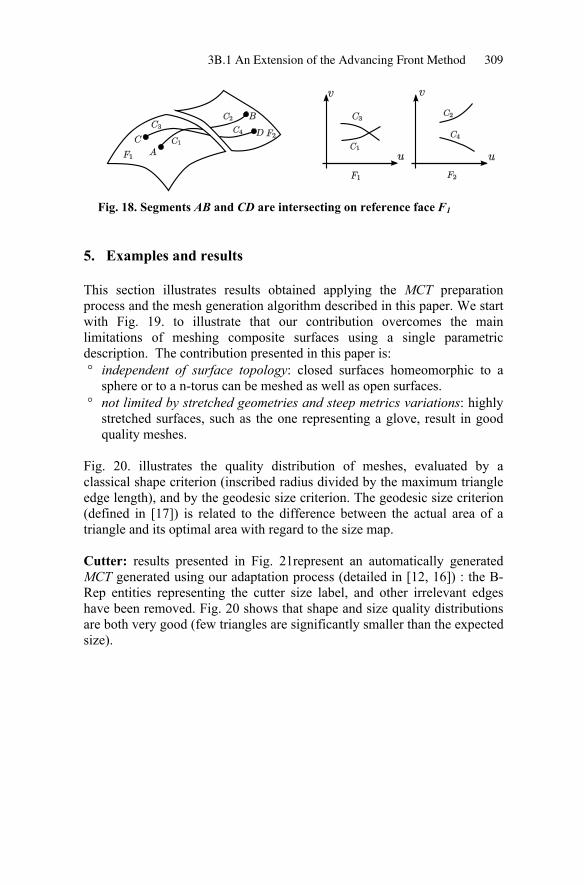
The creation of a triangle during the advancing front method mainly relies on the intersection test between newly created segments and existing segments. The intersection point of two segment is determined by the intersection of their image curves in the parametric space of reference faces (see fig. 18).


Fig. 18. Segments AB and CD are intersecting on reference face F1

5. Examples and results

This section illustrates results obtained applying the MCT preparation process and the mesh generation algorithm described in this paper. We start with Fig. 19. to illustrate that our contribution overcomes the main limitations of meshing composite surfaces using a single parametric description. The contribution presented in this paper is:

independent of surface topology: closed surfaces homeomorphic to a sphere or to a n-torus can be meshed as well as open surfaces. not limited by stretched geometries and steep metrics variations: highly stretched surfaces, such as the one representing a glove, result in good quality meshes.

Fig. 20. illustrates the quality distribution of meshes, evaluated by a classical shape criterion (inscribed radius divided by the maximum triangle edge length), and by the geodesic size criterion. The geodesic size criterion (defined in [17]) is related to the difference between the actual area of a triangle and its optimal area with regard to the size map.

Cutter: results presented in Fig. 21represent an automatically generated MCT generated using our adaptation process (detailed in [12, 16]) : the B-Rep entities representing the cutter size label, and other irrelevant edges have been removed. Fig. 20 shows that shape and size quality distributions are both very good (few triangles are significantly smaller than the expected size).


Fig. 19. Models after topology adaptation and meshes obtained on closed composite surfaces. The remaining MC edge (colored in blue) has been used for the advancing front initialization. For these configurations, approaches based on a mapping into a unique parameterization would likely fail.

Mesh quality

0.00%10.00%20.00%30.00%40.00%50.00%60.00%70.00%80.00%

0.25 0.5 0.75 1

Shape Quality(cutter)Size Quality(cutter)Shape Quality(piston)Size quality(piston)

Fig 20. Quality distribution of the Cutter and Piston meshes


(a)

(b)

(c)

Fig. 21. Mesh generated on a CAD model representing a cutter.

Quarter of piston: fig. 22 shows a piston CAD model, split into one quarter due to symmetry considerations. The original CAD model features many narrow faces and small edges, which are irrelevant for mesh generation. On this sample part, the MCT simplification process [12, 16] operated 60 edges deletions, 62 vertex deletions, and collapsed one edge to a vertex. The number of faces has been reduced from 71 to 21, the number of edges from 182 to 76, and the number of vertices from 113 to 63. Again, size and shape quality distributions are quite satisfying as illustrated in fig. 20.

(a) (b) (c)

Fig. 22. Mesh obtained on a CAD model representing a quarter of piston


6. Conclusion

This paper presents an extension of the advancing front method to surfaces composed of multiple parametric faces, avoiding the construction of a global parameterization and by the way, overcoming the weaknesses of this type of approaches. This extension is intended to be used in the scope of a MCT adaptation procedure that prepares FE models from CAD models. Unlike previous re-parameterization based schemes, the proposed method has no limitations concerning the type and topology of composite surfaces involved.

The main limitation of the current approach concerns its weakness when applied to poorly prepared feature models. For example, a failure in the feature-removal preparation step often cause the presence of small features disturbing the convergence of advancing front mesh generation. The ideal feature-removal algorithm would transform the initial model into a model that conforms to the specified size map. Further work could overcome this weakness by improving the robustness of feature-removal and advancing front mesh generation processes.

Future potential directions in this research include: Extension to elements with higher degree: quadratic triangles (T6) can be easily generated on the exact geometry by inserting a middle node on each segment’s image curve. This method should include a quality criterion to avoid squeezed elements in highly curved zones. The segment-swapping and node moving optimization steps will require quality criteria adapted to curved mesh elements. Extension to mixed-dimensional models: extending feature-removal and MCT preparation algorithms to 3D geometric models mixing curves (meshed with beam elements), surfaces (meshed with shell elements), and solids (meshed with solid elements).

7. Acknowledgements

This study was carried out as part of a project supported by research funding from Québec Nature and Technology Research Fund and by the Natural Sciences and Engineering Research Council of Canada (NSERC).


8. References

1. Halpern, M., Industrial requirements and practices in finite element meshing: a survey of trends, in 6th International Meshing Roundtable. 1997. p. 399--1997.

2. S. Dey, S.S. Mark, and K.G. Marcel, Elimination of the Adverse Effects of Small Model Features by the Local Modification of Automatically Generated Meshes. Engineering with Computers, 1995. 13(3): p. 134--152.

3. Shephard, M.S., M.W. Beall, and R.M.O. Bara, Revisiting the Elimination of the Adverse Effects of Small Model Features in Automatically Generated Meshes, in 7th International Meshing Roundtable. 1998. p. 119-132.

4. Mark, W.B., W. Joe, and S.S. Mark, Accessing CAD Geometry For Mesh Generation, in Proceedings of 12th International Meshing Roundtable, Sandia National Laboratories. 2003.

5. L. Fine, L. Remondini, and J.C. Leon, Automated generation of FEA models through idealization operators. International Journal for Numerical Methods in Engineering, 2000. 49(1): p. 83--108.

6. S. Venkataraman, M. Sohoni, and R. Rajadhyaksha, Removal of blends from boundary representation models, in Proceedings of the seventh ACM symposium on Solid modeling and applications. 2002. p. 83--94.

7. S. Venkataraman, M. Sohoni, and G. Elber, Blend recognition algorithm and applications, in Proceedings of the sixth ACM symposium on Solid modeling and applications. 2001. p. 99--108.

8. S. Venkataraman and M. Sohoni, Reconstruction of feature volumes and feature suppression, in Proceedings of the seventh ACM symposium on Solid modeling and applications. 2002. p. 60--71.

9. K. Y. Lee, et al., A small feature suppression/unsuppression system for preparing B-rep models for analysis, in SPM '05: Proceedings of the 2005 ACM symposium on Solid and physical modeling. 2005: New York, NY, USA. p. 113--124.

10. A. Sheffer, Model simplification for meshing using face clustering. Computer Aided Design, 2001. 33(13): p. 925--934.

11. K. Inoue, et al., Clustering a Large Number of Faces For 2-Dimensional Mesh Generation, in 8th International Meshing Roundtable. 1999. p. 281-292.

12. G. Foucault, et al., A Topological Model for the Representation of Meshing Constraints in the Context of Finite Element Analysis, in Proceedings of ASME 2006 International Design Engineering Technical Conferences and Computers and Information in Engineering Conference. 2006: Philadephia, USA.

13. DL. Marcum, J.G. Unstructured Surface Grid Generation Using Global Mapping and Physical Space Approximation. in 8th International Meshing Roundtable. 1999.

14. F. Noel, Global parameterization of a topological surface defined as a collection of trimmed bi-parametric patches: Application to automatic


mesh construction. International Journal for Numerical Methods in Engineering, 2002. 54(7): p. 965--986.

15. S. H. Lo and T. S. Lau, Mesh generation over curved surfaces with explicit control on discretization error. Engineering Computations, 1998. 15(3): p. 357--373.

16. G Foucault, J-C Cuillière, V François, J-C Léon, R Maranzana,, Towards CAD models automatic simplification for finite element analysis, in 2nd World Congress of Design and Modelling of Mechanical Systems. 2007: Monastir.

17. J-C Cuilliere, An adaptative method for the automatic triangulation of 3D parametric surfaces. Computer Aided Design, 1998. 30: p. 139--149.

18. J-C Cuilliere, Direct method for the automatic discretization of 3D parametric curves. Computer Aided Design, 1997. 29(9): p. 639 - 647.

3b.1 an extension of the advancing front method to ...imr.sandia.gov/papers/imr16/foucault.pdf ·...

Documents