3D AUDIO PLAYBACK THROUGH TWOLOUDSPEAKERS

ByRamin Anushiravani

ECE 499Senior Thesis

Electrical and Computer EngineeringUniversity of Illinois at Urbana Champaign

Urbana, Illinois

Advisor:

Douglas L. Jones

January 10, 2014

To my parents, for their infinite and unconditional love

ii

Abstract

3D sound can reproduce a realistic acoustic environment for binaural recordings through headphonesand loudspeakers. 3D audio playback through loudspeakers is externalized in contrast with headphoneplayback, where the sound localization is inside the head. Playback through loudspeakers, however,requires crosstalk cancellation (XTC). It is known that XTC can add severe spectral coloration to thesignal. One of the more successful XTC filters is the BACCH implemented in Jambox, where the spec-tral coloration is reduced at the cost of lowering the level of XTC. BACCH uses a free field two-pointsource model to derive the XTC filter. In this thesis, Head Related Transfer Function (HRTF)-basedXTC is discussed in comparison with the BACCH filter. The HRTF-based XTC filter considers anindividual’s sound localization frequency responses in a recording room (spectral cues), in addition tothose (ITD and ILD cues) in BACCH. HRTF-based XTC, nevertheless, is individual to one personand works best in an acoustically treated room (e.g., anechoic chamber) for only one sweet spot (it ispossible to create multiple sweet spots for an HRTF-based XTC by tracking the head using Kinect).

Key terms:Binaural recordings Crosstalk Cancellation, Head Related Transfer Function

iii

Acknowledgment

I would like to express my gratitude to my advisor and mentor, Prof. Douglas Jones, for his supportand patience during this project. Prof. Jones has truly been an inspiration to me throughout myacademic life at the University of Illinois. I would also like to acknowledge Michael Friedman fortaking the time to walk me through the project step by step for the past year. The friendship ofNguyen Thi Ngoc Tho is very much appreciated throughout this project, particularly for helping me intaking various acoustic measurements. I would also like to thank Dr. Zhao Shengkui for his valuablecomments on 3D audio playback.

iv

Table of Contents

Chapter 1

Introduction . . . . . . . . . . . . . . . . . . . . . . . . . . . . . . . . . . . . . . . . . . . . . . . . . . . . . . . . . . . . . . . . . . . . . . . . . . . . . . . . . . . . . 11.1 Background . . . . . . . . . . . . . . . . . . . . . . . . . . . . . . . . . . . . . . . . . . . . . . . . . . . . . . . . . . . . . . . . . . . . . . . . . . . . . . . 11.2 Motivation . . . . . . . . . . . . . . . . . . . . . . . . . . . . . . . . . . . . . . . . . . . . . . . . . . . . . . . . . . . . . . . . . . . . . . . . . . . . . . . . 11.3 The Problem of XTC . . . . . . . . . . . . . . . . . . . . . . . . . . . . . . . . . . . . . . . . . . . . . . . . . . . . . . . . . . . . . . . . . . . . . . 2

Chapter 2

Literature Review . . . . . . . . . . . . . . . . . . . . . . . . . . . . . . . . . . . . . . . . . . . . . . . . . . . . . . . . . . . . . . . . . . . . . . . . . . . . . . . . 32.1 Microsoft Research . . . . . . . . . . . . . . . . . . . . . . . . . . . . . . . . . . . . . . . . . . . . . . . . . . . . . . . . . . . . . . . . . . . . . . . . 32.2 OSD . . . . . . . . . . . . . . . . . . . . . . . . . . . . . . . . . . . . . . . . . . . . . . . . . . . . . . . . . . . . . . . . . . . . . . . . . . . . . . . . . . . . . . 42.3 BACCH . . . . . . . . . . . . . . . . . . . . . . . . . . . . . . . . . . . . . . . . . . . . . . . . . . . . . . . . . . . . . . . . . . . . . . . . . . . . . . . . . . . 5

Chapter 3

Fundamentals of XTC . . . . . . . . . . . . . . . . . . . . . . . . . . . . . . . . . . . . . . . . . . . . . . . . . . . . . . . . . . . . . . . . . . . . . . . . . . . .63.1 Free Field Two-Point Source . . . . . . . . . . . . . . . . . . . . . . . . . . . . . . . . . . . . . . . . . . . . . . . . . . . . . . . . . . . . . . .63.2 Metrics . . . . . . . . . . . . . . . . . . . . . . . . . . . . . . . . . . . . . . . . . . . . . . . . . . . . . . . . . . . . . . . . . . . . . . . . . . . . . . . . . . . .73.3 Impulse Responses . . . . . . . . . . . . . . . . . . . . . . . . . . . . . . . . . . . . . . . . . . . . . . . . . . . . . . . . . . . . . . . . . . . . . . . . 83.4 Perfect XTC . . . . . . . . . . . . . . . . . . . . . . . . . . . . . . . . . . . . . . . . . . . . . . . . . . . . . . . . . . . . . . . . . . . . . . . . . . . . . . 9

Chapter 4

Regularization . . . . . . . . . . . . . . . . . . . . . . . . . . . . . . . . . . . . . . . . . . . . . . . . . . . . . . . . . . . . . . . . . . . . . . . . . . . . . . . . . . 124.1 Constant Regularization . . . . . . . . . . . . . . . . . . . . . . . . . . . . . . . . . . . . . . . . . . . . . . . . . . . . . . . . . . . . . . . . . . 124.2 Frequency-Dependent Regularization . . . . . . . . . . . . . . . . . . . . . . . . . . . . . . . . . . . . . . . . . . . . . . . . . . . . . 13

Chapter 5

HRTF-Based XTC . . . . . . . . . . . . . . . . . . . . . . . . . . . . . . . . . . . . . . . . . . . . . . . . . . . . . . . . . . . . . . . . . . . . . . . . . . . . . . 165.1 Sound Localization by Human Auditory System . . . . . . . . . . . . . . . . . . . . . . . . . . . . . . . . . . . . . . . . . . 165.2 HRTF . . . . . . . . . . . . . . . . . . . . . . . . . . . . . . . . . . . . . . . . . . . . . . . . . . . . . . . . . . . . . . . . . . . . . . . . . . . . . . . . . . . .175.3 Perfect HRTF-Based XTC . . . . . . . . . . . . . . . . . . . . . . . . . . . . . . . . . . . . . . . . . . . . . . . . . . . . . . . . . . . . . . . 185.4 Perfect HRTF-Based XTC Simulation . . . . . . . . . . . . . . . . . . . . . . . . . . . . . . . . . . . . . . . . . . . . . . . . . . . . 195.5 Constant Regularization . . . . . . . . . . . . . . . . . . . . . . . . . . . . . . . . . . . . . . . . . . . . . . . . . . . . . . . . . . . . . . . . . . 245.6 Frequency-Dependent Regularization . . . . . . . . . . . . . . . . . . . . . . . . . . . . . . . . . . . . . . . . . . . . . . . . . . . . . 29

Chapter 6

Perceptual Evaluation . . . . . . . . . . . . . . . . . . . . . . . . . . . . . . . . . . . . . . . . . . . . . . . . . . . . . . . . . . . . . . . . . . . . . . . . . . . 336.1 Assumptions . . . . . . . . . . . . . . . . . . . . . . . . . . . . . . . . . . . . . . . . . . . . . . . . . . . . . . . . . . . . . . . . . . . . . . . . . . . . . 336.2 Listening Room Setup . . . . . . . . . . . . . . . . . . . . . . . . . . . . . . . . . . . . . . . . . . . . . . . . . . . . . . . . . . . . . . . . . . . . 336.3 Evaluation . . . . . . . . . . . . . . . . . . . . . . . . . . . . . . . . . . . . . . . . . . . . . . . . . . . . . . . . . . . . . . . . . . . . . . . . . . . . . . . 35

v

Chapter 7

7.1 Summary . . . . . . . . . . . . . . . . . . . . . . . . . . . . . . . . . . . . . . . . . . . . . . . . . . . . . . . . . . . . . . . . . . . . . . . . . . . . . . . . 377.2 Future Work . . . . . . . . . . . . . . . . . . . . . . . . . . . . . . . . . . . . . . . . . . . . . . . . . . . . . . . . . . . . . . . . . . . . . . . . . . . . . 37

References . . . . . . . . . . . . . . . . . . . . . . . . . . . . . . . . . . . . . . . . . . . . . . . . . . . . . . . . . . . . . . . . . . . . . . . . . . . . . . . . . . . . . . 38

Appendix

Matlab Codes . . . . . . . . . . . . . . . . . . . . . . . . . . . . . . . . . . . . . . . . . . . . . . . . . . . . . . . . . . . . . . . . . . . . . . . . . . . . . . . . . . . 40

vi

Chapter 1

1 Introduction

The goal of 3D audio playback through loudspeakers is to re-create a realistic field as if the soundswere recorded at the listener’s ears. 3D Audio can be created either by using Binaural Recordingtechniques [1] or by encoding the Head Related Transfer Function (HRTF) [2] of an individual into astereo signal. 3D Audio must contain the proper Interaural Level Difference (ILD) [3] and InterauralTime Difference (ITD) [4] cues when it is delivered to the listeners. These cues are required by one’sauditory system in order to interpret the 3D image of the sound (3DIS). Any corruptions to ITD andILD cues would result in a severe distortion to the 3DIS. This thesis, discusse different techniques toensure that these cues are delivered to the listener through loudspeakers’ playback that is as accurateas possible.

1.1 Background

There are two major ways to deliver 3D Audio to the listener: headphones and loudspeakers. Whenplayback is through headphones, the ITD and ILD cues for left and right ears are directed to thelisteners’ ears directly, since the signal is transmitted to each ear separately. There are no (very small)reflections in playback through headphones and so it is expected that the 3D audio playback throughheadphones could create a much more realistic field than loudspeakers, where the ITD and ILD cuescan get mixed because both ears can hear the cues meant for the other, and there is also the problemof room reflection when playback is in a non-acoustically treated place.

1.2 Motivation

In practice, however, the 3DIS delivered by the headphone is “internalized”, inside the head, becausethe playback transducers are too close to the ears [5]. A small mismatch between the listener’s HRTFand the one that was used to encode the 3D audio signal, lack of bone-conducted sound (which mightbe fixed using bone-conduction headphones), and the user’s head movement (which might be fixed bytracking the head) are major problems with headphone playback that result in a perception that isinside the head and not realistic.

These problems with headphone playback have been the motivation for research on 3D Audioplayback through loudspeakers, since playback through loudspeakers does not have the issue of inter-nalization.

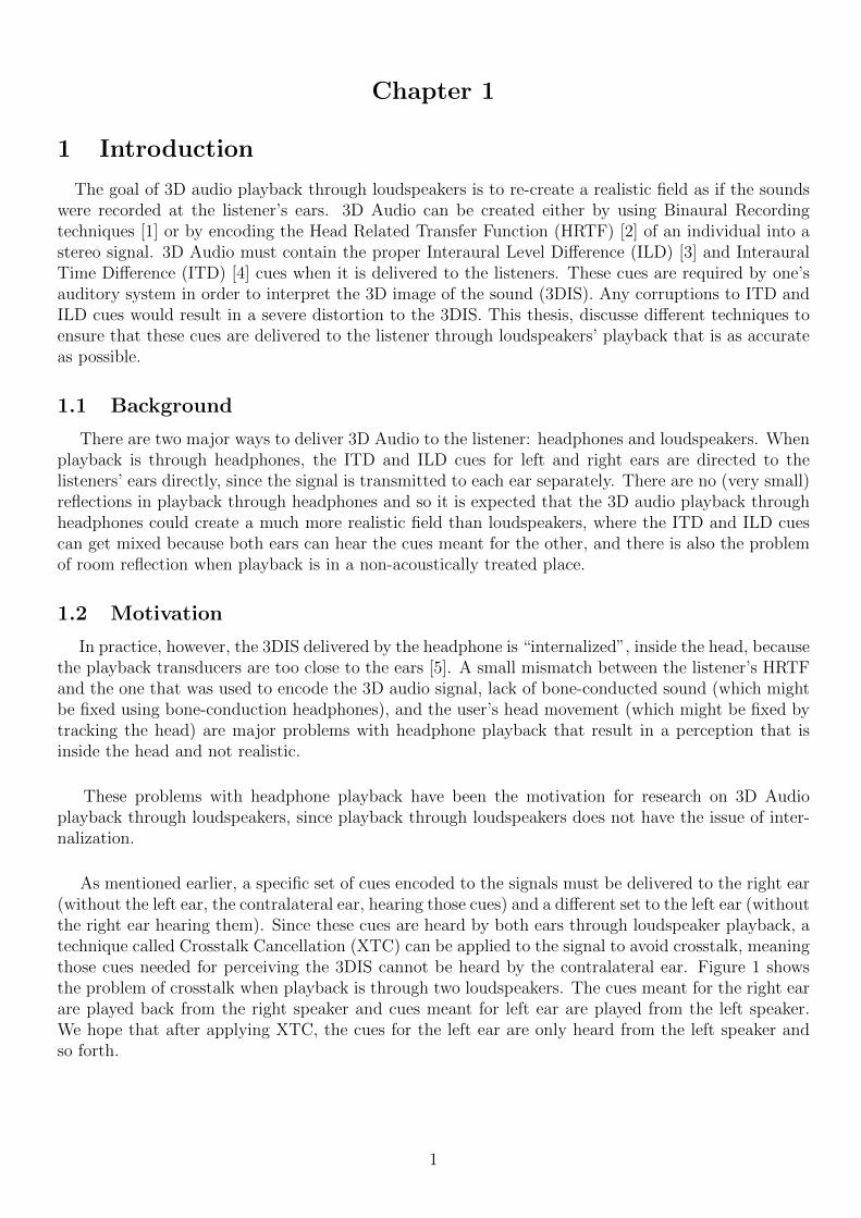
As mentioned earlier, a specific set of cues encoded to the signals must be delivered to the right ear(without the left ear, the contralateral ear, hearing those cues) and a different set to the left ear (withoutthe right ear hearing them). Since these cues are heard by both ears through loudspeaker playback, atechnique called Crosstalk Cancellation (XTC) can be applied to the signal to avoid crosstalk, meaningthose cues needed for perceiving the 3DIS cannot be heard by the contralateral ear. Figure 1 showsthe problem of crosstalk when playback is through two loudspeakers. The cues meant for the right earare played back from the right speaker and cues meant for left ear are played from the left speaker.We hope that after applying XTC, the cues for the left ear are only heard from the left speaker andso forth.

1

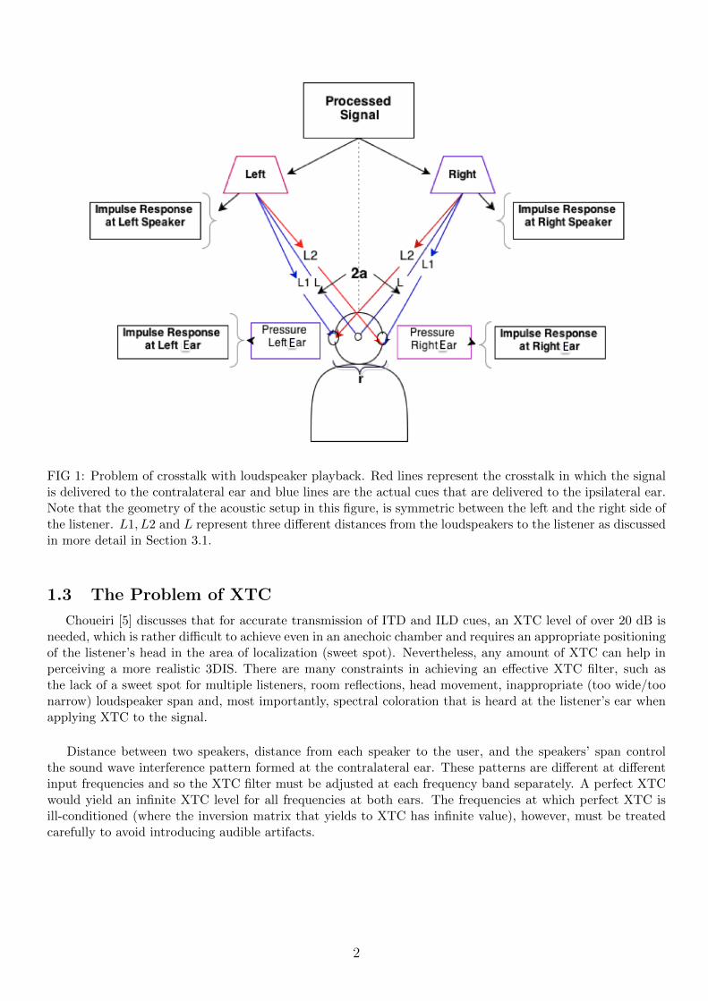
FIG 1: Problem of crosstalk with loudspeaker playback. Red lines represent the crosstalk in which the signalis delivered to the contralateral ear and blue lines are the actual cues that are delivered to the ipsilateral ear.Note that the geometry of the acoustic setup in this figure, is symmetric between the left and the right side ofthe listener. L1, L2 and L represent three different distances from the loudspeakers to the listener as discussedin more detail in Section 3.1.

1.3 The Problem of XTC

Choueiri [5] discusses that for accurate transmission of ITD and ILD cues, an XTC level of over 20 dB isneeded, which is rather difficult to achieve even in an anechoic chamber and requires an appropriate positioningof the listener’s head in the area of localization (sweet spot). Nevertheless, any amount of XTC can help inperceiving a more realistic 3DIS. There are many constraints in achieving an effective XTC filter, such asthe lack of a sweet spot for multiple listeners, room reflections, head movement, inappropriate (too wide/toonarrow) loudspeaker span and, most importantly, spectral coloration that is heard at the listener’s ear whenapplying XTC to the signal.

Distance between two speakers, distance from each speaker to the user, and the speakers’ span controlthe sound wave interference pattern formed at the contralateral ear. These patterns are different at differentinput frequencies and so the XTC filter must be adjusted at each frequency band separately. A perfect XTCwould yield an infinite XTC level for all frequencies at both ears. The frequencies at which perfect XTC isill-conditioned (where the inversion matrix that yields to XTC has infinite value), however, must be treatedcarefully to avoid introducing audible artifacts.

2

Chapter 2

2 Literature Review

Recently, there have been much research on forming optimized XTC filters, such as a Personal 3D audiosystem by Microsoft Research [6], Optimal Source Distribution (OSD) developed by Tekeuchi and Nelson [7],and the BACCH filter developed by Edgar Chouiri [5] which is the main focus of this thesis. Next, I willdiscuss some of these works briefly.

2.1 Microsoft Research

The main focus of “Personal 3D Audio System With Loudspeakers” (P3D) is head tracking. Head trackingcan effectively solve the issue of limited sweet spot and create variable sweet spots based on head movement.The XTC in this section is a matrix inversion of loudspeakers’ natural HRTFs without any regularization.Figure 2 shows the head tracking results in P3D by tracking eyes, lips, ears and the nose.

FIG 2: Head tracking using a regular camera.

The listener’s head movement changes the distance between each ear to the loudspeakers; therefore, avariable time delay is introduced based on the speed of the speed of the sound and the new distance fromeach source to each ear. An adaptive XTC can then be implemented that takes the variable time delay intoconsideration, and so creating an adaptive sweet spot for one individual. Equation 1 shows the transfer matrixfor an individual who is facing two speakers for multiple sweet spots.

XTC =

r0rLz−dLCLL r0rRz−dRCRL

r0rLz−dLCLR

r0rRz−dRCRR

(1)

CLL is the acoustic transfer function from the left speaker to the left ear and CLR is the acoustic transferfunction from the left speaker to the right ear and so on. r0 is the distance between the loudspeakers, rl isthe distance from the left speaker to the left ear and rr is the distance from the right speaker to the rightear. z represents the phase shift (ejw), when dL and dR represent the time delay to each ear which can bemeasured from the geometry of the setup. The inversion matrix will be discussed further in Section 3.4.

3

P3D enables multiple listening sweet spots and is robust to the head movement. The XTC filter in P3D,however, suffers from severe spectral coloration in addition to loss in the dynamic range due to the lack ofregularization. As we will discuss next, one can implement a system where the XTC filter is robust to thehead movement without the need to track the head while maintaining an effective level of XTC at the cost ofsome (very small) spectral coloration.

2.2 OSD

Optimal Source Distribution was developed in 1996 in Southampton Institute of Sound and VibrationResearch (ISVR) at the University of Southampton [8]. OSD involves a pair of “monopole transducers whoseposition varies continuously as a function of frequency” to help the listener localize the sound without applyingsystem inversion to avoid the loss in the dynamic range of the sound. Figure 3 shows a conceptual modelfor when speakers move to right and left for low frequencies and back to the center at higher frequencies. Inpractice OSD uses a minimum of six speakers, where each speaker carries a band-limited range of frequency.

FIG 3: Conceptual model for OST.

Since speakers’ span can change with respect to the frequency, OSD is also able to create multiple sweetspots. OSD is also robust to the reflections and reverberations in the room. Figure 4.a and Figure 4.b showthe set up for OSD [9].

FIG 4.a : Surrounded by six speakers with FIG 4.b: OSD implementation from [9].variable span to create multiple sweet spotsin the room.

OSD is able to overcome many of the issues with common crosstalk cancellation filters such as spectralcoloration, multiple sweet spots and room reverberation. However, OSD is not a practical solution for homeentertainment systems, since it takes a lot of space and it would be very expensive to implement such systems

4

in one’s living room. As shown later in Section 4.2, one can implement some of the great qualities of OSTinto two fixed loudspeakers while maintaining the same level of XTC without loss in the dynamic range.

2.3 BACCH

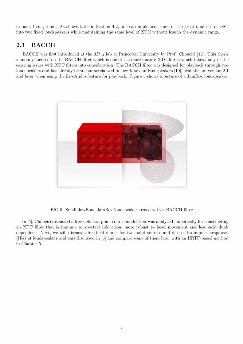
BACCH was first introduced at the 3D3A lab at Princeton University by Prof. Choueiri [13]. This thesisis mainly focused on the BACCH filter which is one of the more mature XTC filters which takes many of theexisting issues with XTC filters into consideration. The BACCH filter was designed for playback through twoloudspeakers and has already been commercialized in JawBone JamBox speakers [10], available on version 2.1and later when using the LiveAudio feature for playback. Figure 5 shows a picture of a JamBox loudspeaker.

FIG 5: Small JawBone JamBox loudspeaker armed with a BACCH filter.

In [5], Choueiri discussed a free-field two-point source model that was analyzed numerically for constructingan XTC filter that is immune to spectral coloration, more robust to head movement and less individual-dependent. Next, we will discuss a free-field model for two point sources and discuss its impulse responses(IRs) at loudspeakers and ears discussed in [5] and compare some of them later with an HRTF-based methodin Chapter 5.

5

Chapter 3

3 Fundamentals of XTC

There are different methods to form an XTC filter for two speakers. In this thesis, two major methods arereviewed, a numerical method using wave equations as done in BACCH filter and an HRTF-based method.In this section, some of the important acoustic equations related to the XTC are reviewed as shown in [5, 8].

3.1 Free-Field Two-Point Source

In this section, an analytical model of a two-point source model in free field as shown earlier in Figure 1 isdiscussed.

Pressure from a simple point source in a homogenous medium at distance L can be calculated as follows[14],

P (L, t) =(A

L)ej(wt−kL) (2)

where P is the air pressure located at distance L and at time t from the point source. w is the angularvelocity of the pulsating source, k is the wavenumber, and j is an imaginary unit. A is a factor that can befind using appropriate boundary condition as

A =p0q

4π(3)

where p0 is the air density and q is the source strength. Equation (3) represents the pressure in the timedomain; this can be easily converted back to the frequency domain as follows

P (L,w) =(jwA

L)e−jkL (4)

For convenience we can define

V =jwA

L(5)

V is the derivative ofAL in frequency domain; therefore, it is defined as the rate of air density flow from the

point source.

Given Equation 4 and Figure 1, we can define the pressure at each ear in the frequency domain as follows,

PL = VLe−jkL1

L1+ VR

e−jkL2

L2(6)

PR = VRe−jkL1

L1+ VL

e−jkL2

L2(7)

where L1 is the distance between the speaker and the ipsilateral ear (LL, RR), L2 is the distance betweenthe speaker and the contralateral ear (LR, RL), VL is the rate of air flow from the left speaker, and VR is therate of air flow from the right speaker. The second term in both equations 6 and 7 represent the pressure at

6

the contralateral ear, the crosstalk pressure. Using the geometry shown in Figure 1, we can calculate L1 andL2 in terms of L,

L1 =

√L2 +

r

2

2− rL sin(α) (8)

L2 =

√L2 +

r

2

2+ rL sin(α) (9)

where L is the distance between each speaker to the listener’s head, r is the distance between the listener’sleft and right ears, and 2α is defined as the speakers’ span with respect to the listener’s head. For conveniencewe can define,

g =L1

L2, ∆L = L2 − L1 (10)

where g defines the ratio between the ipsilateral distance to the contralateral distance. Normally for a far-fieldlistening room, this ratio is about 0.985 [5]. The time it takes for the sound to travel from the speaker to thecontralateral ear is delayed by ∆L. The time delay is then,

τ =∆L

C(11)

where C is the speed of sound at room temperature or approximately 340.3 m/s.

Equations 1 through 11 describe the pressure in a free-field two-point source model for the setup shownin Figure 1. In the next section, we will define a system based on these equations that will take the soundpressures at the loudspeakers and ears into consideration when constructing the XTC filter as shown in Figure1.

3.2 Metrics

Using Equations 6 and 7 we can form the following matrices,[PLPR

]= α

[1 ge−jwτ

ge−jwτ 1

] [VLVR

](12)

where α is defined ase−jwL1/C

L1 . α is the time it takes for the signal to travel from the speaker to the ipsilateralear divided by L1. Consider PL for example, the pressure at the left ear is the rate of air flow at the right eardelayed by α plus the rate of air pressure flow at the right speaker delayed by α, also delayed by τ and thenlowered by g. The diagonal terms in Equation 11 describe the ipsilateral pressure and the off-diagonal elementsdescribe the crosstalk pressure at the contralateral ear. VL and VR are the pressures at the loudspeakers inthe frequency domain which can be calculated as follows,[

VLVR

]=

[HLL HLR

HRL HRR

] [DL

DR

](13)

where HLL is the left speaker impulse response recorded at the left ear, HLR is the left speaker impulseresponse recorded at the right ear and so forth. DL is the left recorded signal and DR is the right recordedsignal. Given Equation (13), we can write Equation (12) as follows,

[PLPR

]= α

[1 ge−jwτ

ge−jwτ 1

] [HLL HLR

HRL HRR

] [DL

DR

](14)

For convenience we define

7

N =

[1 ge−jwτ

ge−jwτ 1

](15)

where N is the listening room setup transfer matrix delayed by α. And,

H =

[HLL HLR

HRL HRR

](16)

where the H’s are the speakers’ impulse response due to their placements. H can be measured by extractingthe impulse response in front of the speaker as discussed in Chapter 5. D represents the desired recordedsignal encoded with binaural cues.

D =

[DL

DR

](17)

Next we will define a performance matrix [5],

R =

[RLL RLRRRL RRR

]= NH (18)

where R represents the natural HRTF of speakers due to its location with respect to the listener and eachother, including the distance between the speakers and the listener. R is basically a set of impulse responsesthat exist in the listening room due to the positioning of the speakers with respect to the listener. R can bemeasured in the room by extracting the impulse response at the listener’s ears.The final pressure at the ear is then,

P = αRD (19)

We now have enough information to calculate and simulate the impulse responses at the speakers and atthe listener’s ears.

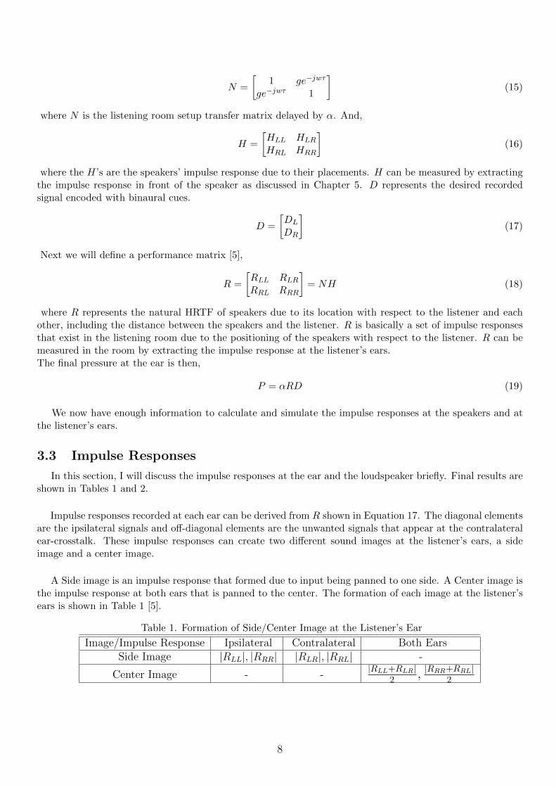
3.3 Impulse Responses

In this section, I will discuss the impulse responses at the ear and the loudspeaker briefly. Final results areshown in Tables 1 and 2.

Impulse responses recorded at each ear can be derived from R shown in Equation 17. The diagonal elementsare the ipsilateral signals and off-diagonal elements are the unwanted signals that appear at the contralateralear-crosstalk. These impulse responses can create two different sound images at the listener’s ears, a sideimage and a center image.

A Side image is an impulse response that formed due to input being panned to one side. A Center image isthe impulse response at both ears that is panned to the center. The formation of each image at the listener’sears is shown in Table 1 [5].

Table 1. Formation of Side/Center Image at the Listener’s Ear

Image/Impulse Response Ipsilateral Contralateral Both EarsSide Image |RLL|, |RRR| |RLR|, |RRL| -

Center Image - -|RLL+RLR|

2 , |RRR+RRL|2

8

Another important frequency response is the one at the loudspeakers. The result is shown in Table 2 below.

Table 2. Formation of Side/Center Image at the Loudspeaker

Image/Impulse Response Ipsilateral Contralateral Both SidesSide Image |HLL|, |HRR| |HLR|, |HRL| -

Center Image - -|HLL+HLR|

2 , |HRR+HRL|2

As can be seen, once the ipsilateral and the contralateral signals interfere, the side image transforms to acenter image. There are also sound images that can be created due to signals being in-phase and out-of-phaseat the loudspeaker. The images formed at the loudspeakers are shown in Table 3.

Table 3. Formation of In/Out of Phase Images at the Loudspeaker, S

Image/Impulse Response Ipsilateral ContralateralIn-Phase Image |HLL +HRR| |HLR +HLR|

Out-of-Phase Image |HLL −HRR| |HLR −HLR|

An in-phase image is double the center image. This is of course because the signal was divided into twoequal signals at the center. As shown in [5], it is more useful to find the maximum phase since there will bedifferent phase components based on the system setup.

S = max[S[in−phase], S[out−of−phase]] (20)

where S is the maximum amplitude impulse response we expect to see at the loudspeakers. Another importantfactor mentioned in [5] is the crosstalk-cancellation spectrum,

X(w) =|RLL||RRL|

(21)

This can be easily calculated by dividing the impulse response at the ear by the contralateral ear. The XTCspectrum can also be defined as the division of the side image by the center image described in Table 1.

3.4 Perfect XTC

A perfect XTC cancels all the crosstalk at both ears for all the frequencies (X = ∞). As shown inEquation 18, the final pressure at each ear is the desired recorded signal multiplied by R in the frequencydomain (separately for the left and right channels) and delayed by α. It is clear that to transmit the desiredsignal without crosstalk, R must be equal to the identity matrix. Looking back at Equation (17) we thenhave,

HP = N−1 =1

1− g2e−2jwτc

[1 −ge−jwτc

−ge−jwτc 1

]=

1

1− g2e−2jk∆L

[1 −ge−jk∆L

−ge−jk∆L 1

](22)

where HP represents the Perfect XTC. For far distance, when l� ∆r, ∆L = ∆r sin(α). So, we can re-writeEquation (22) in terms of the distance between left and right ears, speaker span and g.

HP =1

1− g2e−2jk∆rsin(α)

[1 −ge−jk∆rsin(α)

−ge−jk∆rsin(α) 1

](23)

Given Equations 22 and 23, we can solve for every other impulse responses in Tables 1 to 3 as calculated in[5]. As an example, the maximum amplitude frequency response at the loudspeaker would be the following,

S = max

(1√

g2 + 2g.cos(wτc)) + 1,

1√g2 − (2g.cos(wτc)) + 1

)(24)

9

where wτc = k∆L = k∆rsin(α) =2πf∆rsin(α)

cs. Obviously, frequency depends on the speakers’ span (α) and

the only variable that can be controlled by the user in a normal listening room is the speakers’ span. Solvingfor α we have,

α(f) = sin−1(cswτc

2πf∆r) (25)

It can be shown that wτc must be equal to nπ/2 to avoid ill-conditioned frequencies (frequencies where thesystem inversion leads to spectral coloration). Therefore we have,

α(f) = sin−1(ncs

4f∆r) (26)

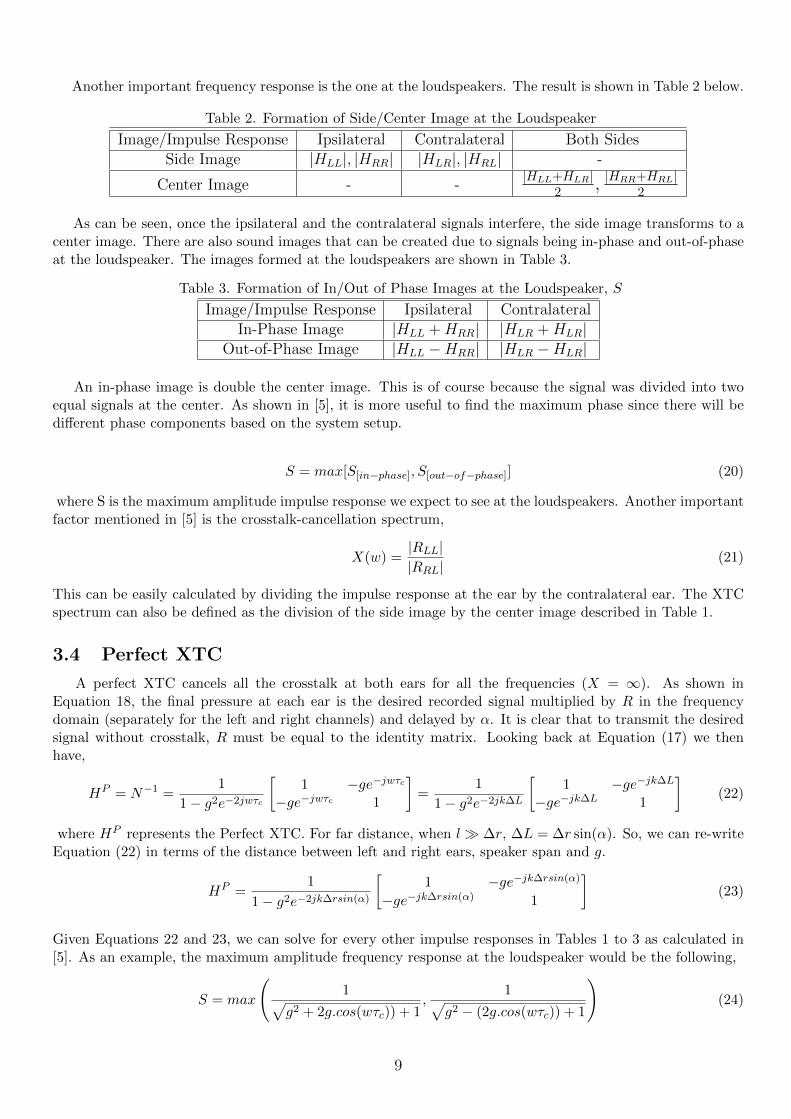
Equation 26 is the basis of OSD explained in Section 2.2, where the loudspeakers’ span changes with frequencyto ensure a high level of XTC while avoiding spectral coloration. Figure 6 shows the side image, center imageand the maximum amplitude frequency response at the loudspeaker when PXTC is applied to the system.

FIG 6: Frequency response at the loudspeaker for PXTC.

The green curve SP represents the maximum amplitude spectrum at the loudspeaker. The blue and redcurves represent SSideImage and SCenterImage at the loudspeaker when PXTC is applied to the system. Thecharacteristics for the listening room setup in Figure 6 are,

g = 0.985, τc = 65 us, L = 1.6 m and 2α = 18◦

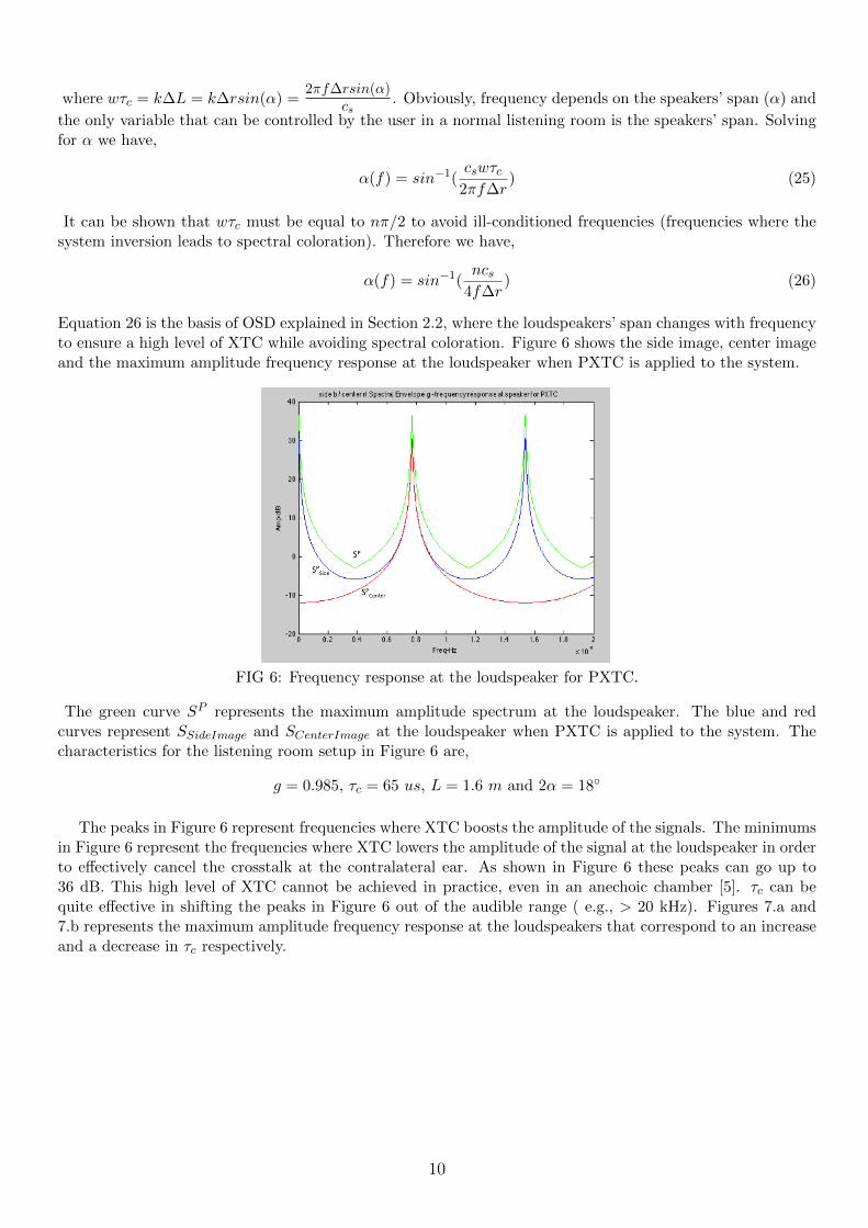
The peaks in Figure 6 represent frequencies where XTC boosts the amplitude of the signals. The minimumsin Figure 6 represent the frequencies where XTC lowers the amplitude of the signal at the loudspeaker in orderto effectively cancel the crosstalk at the contralateral ear. As shown in Figure 6 these peaks can go up to36 dB. This high level of XTC cannot be achieved in practice, even in an anechoic chamber [5]. τc can bequite effective in shifting the peaks in Figure 6 out of the audible range ( e.g., > 20 kHz). Figures 7.a and7.b represents the maximum amplitude frequency response at the loudspeakers that correspond to an increaseand a decrease in τc respectively.

10

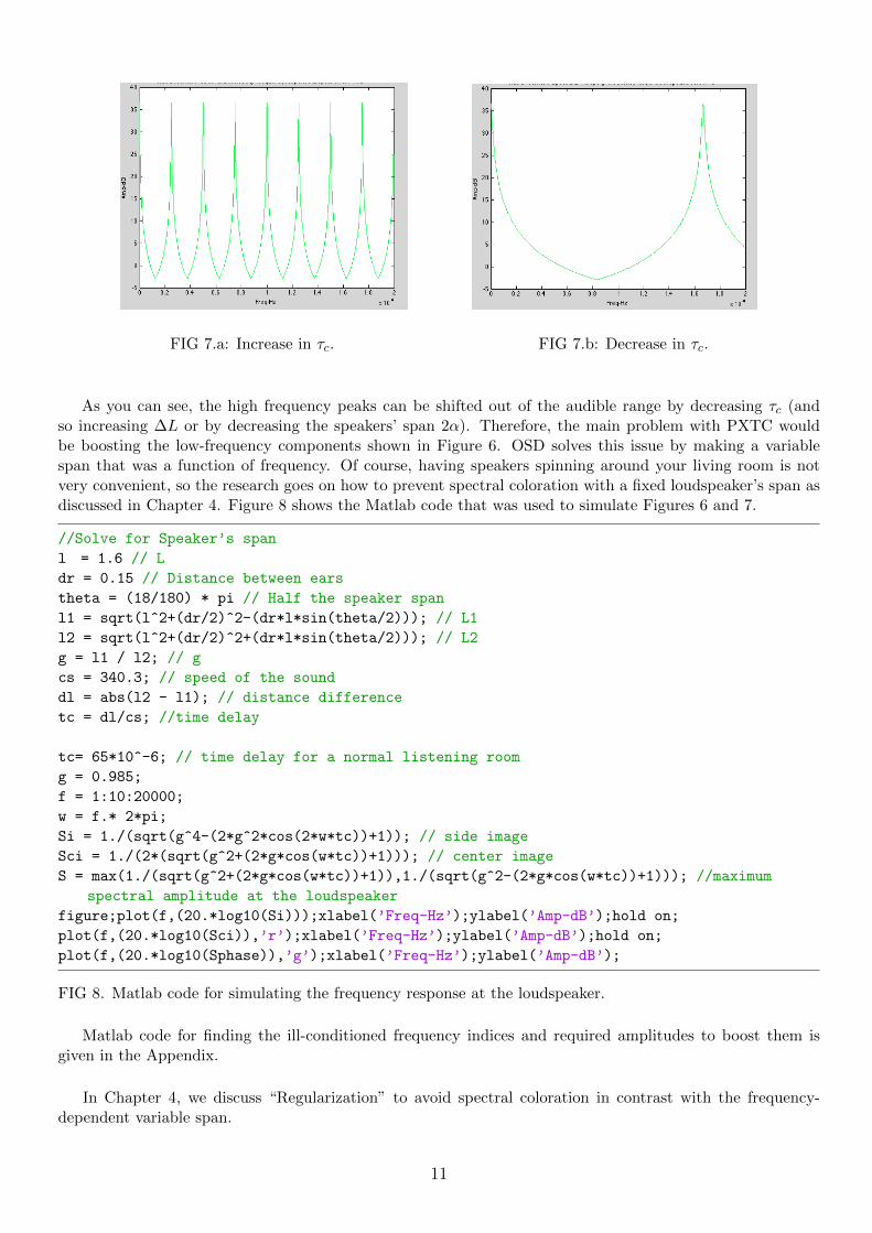
FIG 7.a: Increase in τc. FIG 7.b: Decrease in τc.

As you can see, the high frequency peaks can be shifted out of the audible range by decreasing τc (andso increasing ∆L or by decreasing the speakers’ span 2α). Therefore, the main problem with PXTC wouldbe boosting the low-frequency components shown in Figure 6. OSD solves this issue by making a variablespan that was a function of frequency. Of course, having speakers spinning around your living room is notvery convenient, so the research goes on how to prevent spectral coloration with a fixed loudspeaker’s span asdiscussed in Chapter 4. Figure 8 shows the Matlab code that was used to simulate Figures 6 and 7.

//Solve for Speaker’s span

l = 1.6 // L

dr = 0.15 // Distance between ears

theta = (18/180) * pi // Half the speaker span

l1 = sqrt(l^2+(dr/2)^2-(dr*l*sin(theta/2))); // L1

l2 = sqrt(l^2+(dr/2)^2+(dr*l*sin(theta/2))); // L2

g = l1 / l2; // g

cs = 340.3; // speed of the sound

dl = abs(l2 - l1); // distance difference

tc = dl/cs; //time delay

tc= 65*10^-6; // time delay for a normal listening room

g = 0.985;

f = 1:10:20000;

w = f.* 2*pi;

Si = 1./(sqrt(g^4-(2*g^2*cos(2*w*tc))+1)); // side image

Sci = 1./(2*(sqrt(g^2+(2*g*cos(w*tc))+1))); // center image

S = max(1./(sqrt(g^2+(2*g*cos(w*tc))+1)),1./(sqrt(g^2-(2*g*cos(w*tc))+1))); //maximum

spectral amplitude at the loudspeaker

figure;plot(f,(20.*log10(Si)));xlabel(’Freq-Hz’);ylabel(’Amp-dB’);hold on;

plot(f,(20.*log10(Sci)),’r’);xlabel(’Freq-Hz’);ylabel(’Amp-dB’);hold on;

plot(f,(20.*log10(Sphase)),’g’);xlabel(’Freq-Hz’);ylabel(’Amp-dB’);

FIG 8. Matlab code for simulating the frequency response at the loudspeaker.

Matlab code for finding the ill-conditioned frequency indices and required amplitudes to boost them isgiven in the Appendix.

In Chapter 4, we discuss “Regularization” to avoid spectral coloration in contrast with the frequency-dependent variable span.

11

Chapter 4

4 Regularization

Regularization is a technique that reduces the effect of the ill-conditioned frequencies at the cost of losingsome amount of XTC. In Equation (23), we see that the fraction next to the speaker’s natural HRTF is thereason we have ill-conditioned frequencies at the first place. For example, there might be a frequency at whichthe amplitude for this fraction (determinant of N) is very small, therefore, taking the inverse of this fractionmight result in boosting the signal at that specific frequency to a very large value. To avoid this issue, onecan shift the magnitude of this determinant by a small value while keeping the phase to avoid introducingsevere spectral coloration to the signal.

4.1 Constant Regularization

Constant regularization shifts the magnitude at every frequency bins with an equal amplitude. As shownin [5], we can approximate the inversion matrix from Equation (22), using linear least-square aprroximationas follows,

Hβ = [NHN + βI]−1NH (27)

where Hβ represents the regularized XTC and the subscript H is the Hermition operator (conjugate transpose)and β is the regularization factor. It can be shown that increase in β would reduce the artifacts at the costof decreasing the XTC level. Given Equation 27, we can once again derive all the equations in Tables 1 to3. For example, the maximum amplitude frequency response at the loudspeaker for constant regularizationwould be

Sβ = max

( √g2 + 2g.cos(w.tc) + 1

g2 + 2g.cos(wtc)) + β + 1,

√g2 − 2g.cos(w.tc) + 1

g2 − (2g.cos(w.tc)) + β + 1

)(28)

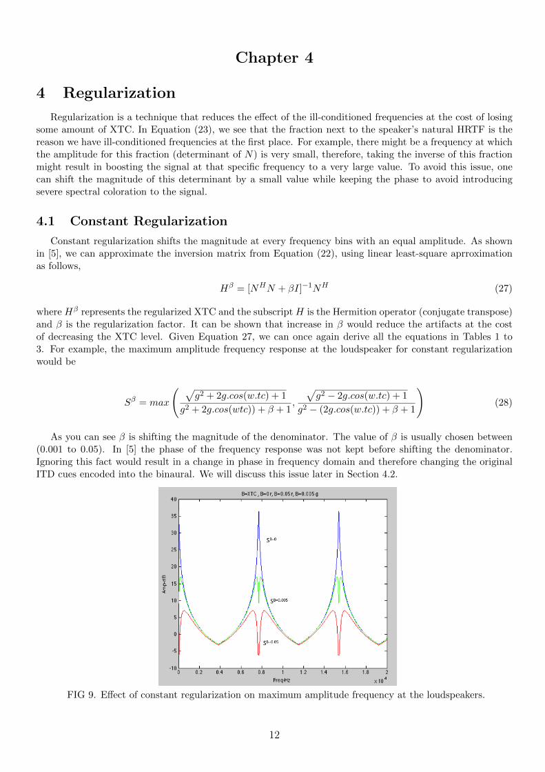
As you can see β is shifting the magnitude of the denominator. The value of β is usually chosen between(0.001 to 0.05). In [5] the phase of the frequency response was not kept before shifting the denominator.Ignoring this fact would result in a change in phase in frequency domain and therefore changing the originalITD cues encoded into the binaural. We will discuss this issue later in Section 4.2.

FIG 9. Effect of constant regularization on maximum amplitude frequency at the loudspeakers.

12

As you can see in Figure 9, even a small regularization factor decreases the XTC level at the ill-conditionedfrequency by almost 20 dB. One of the problems with the constant regularization, as seen in Figure 9, is theformation of doublet peaks in the frequency response. The first doublet at 0 Hz is perceived as a wide-bandlow frequency rolloff and the two other two doublet are perceived as narrow-band artifacts at high frequenciesdue to the human logarithmic frequency perception [5]. As mentioned earlier, the high frequency peaks canbe shifted out the audible range by changing the listening room set up; therefore the main problem is the lowfrequency peaks. It worth noting that the low frequency boost in PXTC transformed in to low frequency rolloff at constant regularization.

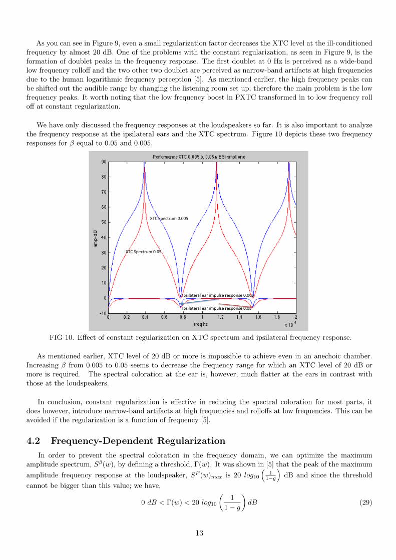
We have only discussed the frequency responses at the loudspeakers so far. It is also important to analyzethe frequency response at the ipsilateral ears and the XTC spectrum. Figure 10 depicts these two frequencyresponses for β equal to 0.05 and 0.005.

FIG 10. Effect of constant regularization on XTC spectrum and ipsilateral frequency response.

As mentioned earlier, XTC level of 20 dB or more is impossible to achieve even in an anechoic chamber.Increasing β from 0.005 to 0.05 seems to decrease the frequency range for which an XTC level of 20 dB ormore is required. The spectral coloration at the ear is, however, much flatter at the ears in contrast withthose at the loudspeakers.

In conclusion, constant regularization is effective in reducing the spectral coloration for most parts, itdoes however, introduce narrow-band artifacts at high frequencies and rolloffs at low frequencies. This can beavoided if the regularization is a function of frequency [5].

4.2 Frequency-Dependent Regularization

In order to prevent the spectral coloration in the frequency domain, we can optimize the maximumamplitude spectrum, Sβ(w), by defining a threshold, Γ(w). It was shown in [5] that the peak of the maximum

amplitude frequency response at the loudspeaker, SP (w)max is 20 log10

(1

1−g

)dB and since the threshold

cannot be bigger than this value; we have,

0 dB < Γ(w) < 20 log10

(1

1− g

)dB (29)

13

If SP (w) is bigger than Γ(w) then Sβ(w) is made to be equal to Γ(w) at that frequency bin, otherwiseSβ(w) would be equal to SP (w). Looking back at Equation 28, if we solve for β when SP (w) = Γ(w), thenwe have,

β1(w) = −g2 + 2gcos(wτc) +

√g2 − 2gcos(wτc) + 1

10Γ

20

− 1 (30)

β2(w) = −g2 − 2gcos(wτc) +

√g2 + 2gcos(wτc) + 1

10Γ

20

− 1 (31)

It was shown in [5] that β1(w) is applied when the maximum amplitude spectrum is the out-of-phase com-ponent, and β2(w) is used when the in-phase component is the maximum value (Eq.20). We summarize theresults in Table 4.

Table. 4, Formation of In/Out of Phase Images at the Loudspeaker

Condition I/Condition II SoP > Si

P SiP > So

P

SP (w) > 10Γ

20β = β1(w) β = β2(w)

SP (w) > 10Γ

20β = 0 β = 0

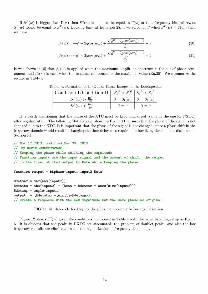
It is worth mentioning that the phase of the XTC must be kept unchanged (same as the one for PXTC)after regularization. The following Matlab code, shown in Figure 11, ensures that the phase of the signal is notchanged due to the XTC. It is important that the phase of the signal is not changed, since a phase shift in thefrequency domain would result in changing the time-delay cues required for localizing the sound as discussed inSection 5.1.

// Nov 12,2013, modified Nov 30, 2013

// by Ramin Anushiravani

// Keeping the phase while shifting the magnitude

// Function inputs are the input signal and the amount of shift, the output

// is the final shifted output by Beta while keeping the phase.

function output = bkphase(input1,input2,Beta)

Bdetmax = max(abs(input2));

Bdetabs = abs(input2) + (Beta * Bdetmax * ones(size(input2)));

Bdetang = angle(input1);

output = (Bdetabs).*(exp(1j*Bdetang));

// create a response with the new magnitude but the same phase as original.

FIG 11. Matlab code for keeping the phase components before regularization.

Figure 12 shows Sβ(w) given the conditions mentioned in Table 4 with the same listening setup as Figure6. It is obvious that the peaks in PXTC are attenuated, the problem of doublet peaks, and also the lowfrequency roll offs are eliminated when the regularization is frequency dependent.

14

FIG 12: Sβ(w) is the blue curve. The red curve depicts the peaks at the PXTC as shown in Figure 6.

In this section we have discussed the advantages of frequency-dependent regularization over constantregularization. In Chapter 5, we will discuss the HRTF-Based XTC in comparison with the Free Field Two-Point Source model in Section 3.1.

15

Chapter 5

5 HRTF-Based XTC

In the previous sections, we discussed the fundamental of XTC using acoustic wave equations and theadvantages of applying regularization to the XTC filter. In this chapter, we will discuss the HRTF-BasedXTC which includes spectral cues, in addition to interaural time difference (ITD) and the interaural leveldifference (ILD) cues discussed in [5].

5.1 Sound Localization by Human Auditory System

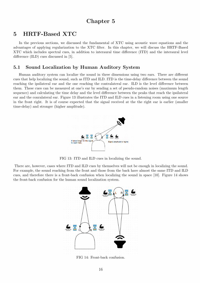
Human auditory system can localize the sound in three dimensions using two ears. There are differentcues that help localizing the sound, such as ITD and ILD. ITD is the time-delay difference between the soundreaching the ipsilateral ear and the one reaching the contralateral ear. ILD is the level difference betweenthem. These cues can be measured at one’s ear by sending a set of pseudo-random noises (maximum lengthsequence) and calculating the time delay and the level difference between the peaks that reach the ipsilateralear and the conralateral ear. Figure 13 illustrates the ITD and ILD cues in a listening room using one sourcein the front right. It is of course expected that the signal received at the the right ear is earlier (smallertime-delay) and stronger (higher amplitude).

FIG 13: ITD and ILD cues in localizing the sound.

There are, however, cases where ITD and ILD cues by themselves will not be enough in localizing the sound.For example, the sound reaching from the front and those from the back have almost the same ITD and ILDcues, and therefore there is a front-back confusion when localizing the sound in space [10]. Figure 14 showsthe front-back confusion for the human sound localization system.

FIG 14: Front-back confusion.

16

In addition to ITD and ILD cues, there are also the spectral cues which also include the head-shadow effect,outer ear shape and the room impulse response (HRTF).

5.2 HRTF

The Head Related Transfer Function (HRTF) is an individual’s sound localization transfer function fora point in space. HRTF includes information about a sound travelling from a point to the outer ears of anindividual. Given a set of HRTFs, one can create sounds coming from different angles by multiplying anarbitrary sound with the HRTFs for that point in the frequency domain, which is equivalent to convolving theinput signal with the Head Related Impulse Response (HRIR). Equation 32 shows the 3D audio reconstructionof an arbitrary mono input signal using HRTFs in the frequency domain.[

OutL(α)OutR(α)

]=[Input Input

].

[HRTFL(α)HRTFR(α)

](32)

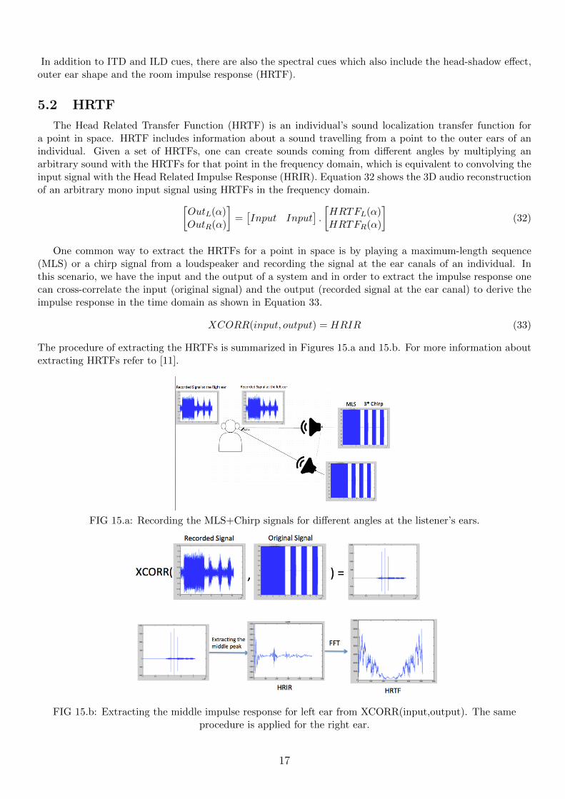
One common way to extract the HRTFs for a point in space is by playing a maximum-length sequence(MLS) or a chirp signal from a loudspeaker and recording the signal at the ear canals of an individual. Inthis scenario, we have the input and the output of a system and in order to extract the impulse response onecan cross-correlate the input (original signal) and the output (recorded signal at the ear canal) to derive theimpulse response in the time domain as shown in Equation 33.

XCORR(input, output) = HRIR (33)

The procedure of extracting the HRTFs is summarized in Figures 15.a and 15.b. For more information aboutextracting HRTFs refer to [11].

FIG 15.a: Recording the MLS+Chirp signals for different angles at the listener’s ears.

FIG 15.b: Extracting the middle impulse response for left ear from XCORR(input,output). The sameprocedure is applied for the right ear.

17

5.3 Perfect HRTF-Based XTC

Looking back at Figure 1, one can extract the impulse response at the ipsilateral and contralateral (XT)ear using HRTFs. Equation 13 can then be written as,[

OutLOutR

]=

[HRTFLL HRTFLRHRTFRL HRTFRR

] [InLInR

](34)

[HRTFLL HRTFLRHRTFRL HRTFRR

]= HS (35)

where Out is the signal received at the ear and In is the input to the loudspeakers ( e.g., 3D audio) bothin the frequency domain. The HRTF matrix is comprised of the frequency responses existing in the listeningroom due to the geometry of the setup, listener’s source localization system and the room impulse response.One can then extract the impulse response at the listener’s ears for that specific listening room in order tocancel the crosstalk in that room for that individual. The same fundamentals are applied to HRTF-basedXTC as those applied to the two-point source free-field model in Section 3. A Perfect HRTF-Based XTC canbe derived similar to Equation 22 as shown below,

XTCPHRTF = H−1S =

[HRTFLL HRTFLRHRTFRL HRTFRR

]−1

(36)

where XTCPHRTF is the perfect HRTF-Based XTC. Expanding this equation gives,

1

HRTFLL.HRTFRR −HRTFLR.HRTFRL

[HRTFRR −HRTFLR−HRTFRL HRTFLL

](37)

The first term in Equation 37, is 1Determinant . This term must be treated carefully to avoid spectral coloration

in the XTC. As an example, Figure 16 depicts this term for an individual’s HRTF recorded in an officeenvironment.

FIG 16: Deteminant of Equation 35 in the frequency domain.

As can be seen for some frequencies, the amplitude of the Determinant is lower than -20 dB (20 log(0.1) =−20 dB). When taking the inverse of the Determinant, the amplitude at these frequencies are amplified byan order of 10 to 100. This of course would introduce a severe spectral coloration to the signal, since some ofthe frequencies are over-amplified due to the very high level of XTC required at that frequency.

For a perfect XTC we expect to have,

RS = H−1S ∗XTC

PHRTF =

[HRTFLL HRTFLRHRTFRL HRTFRR

]∗[HRTFLL HRTFLRHRTFRL HRTFRR

]−1

=

[1 00 1

](38)

18

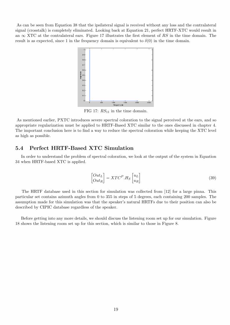
As can be seen from Equation 38 that the ipsilateral signal is received without any loss and the contralateralsignal (crosstalk) is completely eliminated. Looking back at Equation 21, perfect HRTF-XTC would result inan ∞ XTC at the contralateral ears. Figure 17 illustrates the first element of RS in the time domain. Theresult is as expected, since 1 in the frequency domain is equivalent to δ(0) in the time domain.

FIG 17: RS11 in the time domain.

As mentioned earlier, PXTC introduces severe spectral coloration to the signal perceived at the ears, and soappropriate regularization must be applied to HRTF-Based XTC similar to the ones discussed in chapter 4.The important conclusion here is to find a way to reduce the spectral coloration while keeping the XTC levelas high as possible.

5.4 Perfect HRTF-Based XTC Simulation

In order to understand the problem of spectral coloration, we look at the output of the system in Equation34 when HRTF-based XTC is applied.

[OutLOutR

]= XTCP .HS

[uLuR

](39)

The HRTF database used in this section for simulation was collected from [12] for a large pinna. Thisparticular set contains azimuth angles from 0 to 355 in steps of 5 degrees, each containing 200 samples. Theassumption made for this simulation was that the speaker’s natural HRTFs due to their position can also bedescribed by CIPIC database regardless of the speaker.

Before getting into any more details, we should discuss the listening room set up for our simulation. Figure18 shows the listening room set up for this section, which is similar to those in Figure 8.

19

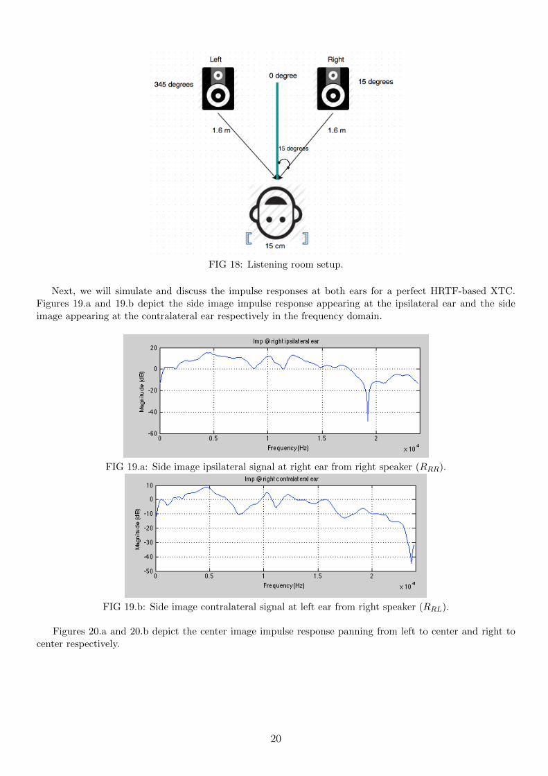
FIG 18: Listening room setup.

Next, we will simulate and discuss the impulse responses at both ears for a perfect HRTF-based XTC.Figures 19.a and 19.b depict the side image impulse response appearing at the ipsilateral ear and the sideimage appearing at the contralateral ear respectively in the frequency domain.

FIG 19.a: Side image ipsilateral signal at right ear from right speaker (RRR).

FIG 19.b: Side image contralateral signal at left ear from right speaker (RRL).

Figures 20.a and 20.b depict the center image impulse response panning from left to center and right tocenter respectively.

20

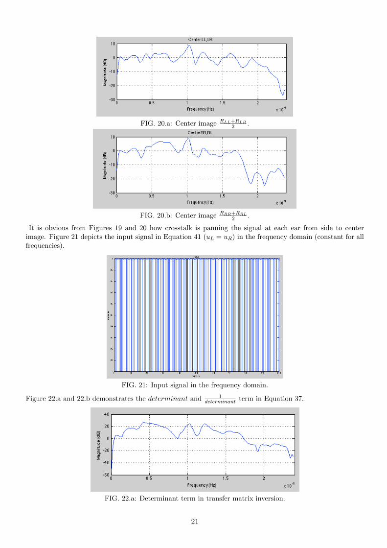
FIG. 20.a: Center image RLL+RLR2 .

FIG. 20.b: Center image RRR+RRL2 .

It is obvious from Figures 19 and 20 how crosstalk is panning the signal at each ear from side to centerimage. Figure 21 depicts the input signal in Equation 41 (uL = uR) in the frequency domain (constant for allfrequencies).

FIG. 21: Input signal in the frequency domain.

Figure 22.a and 22.b demonstrates the determinant and 1determinant term in Equation 37.

FIG. 22.a: Determinant term in transfer matrix inversion.

21

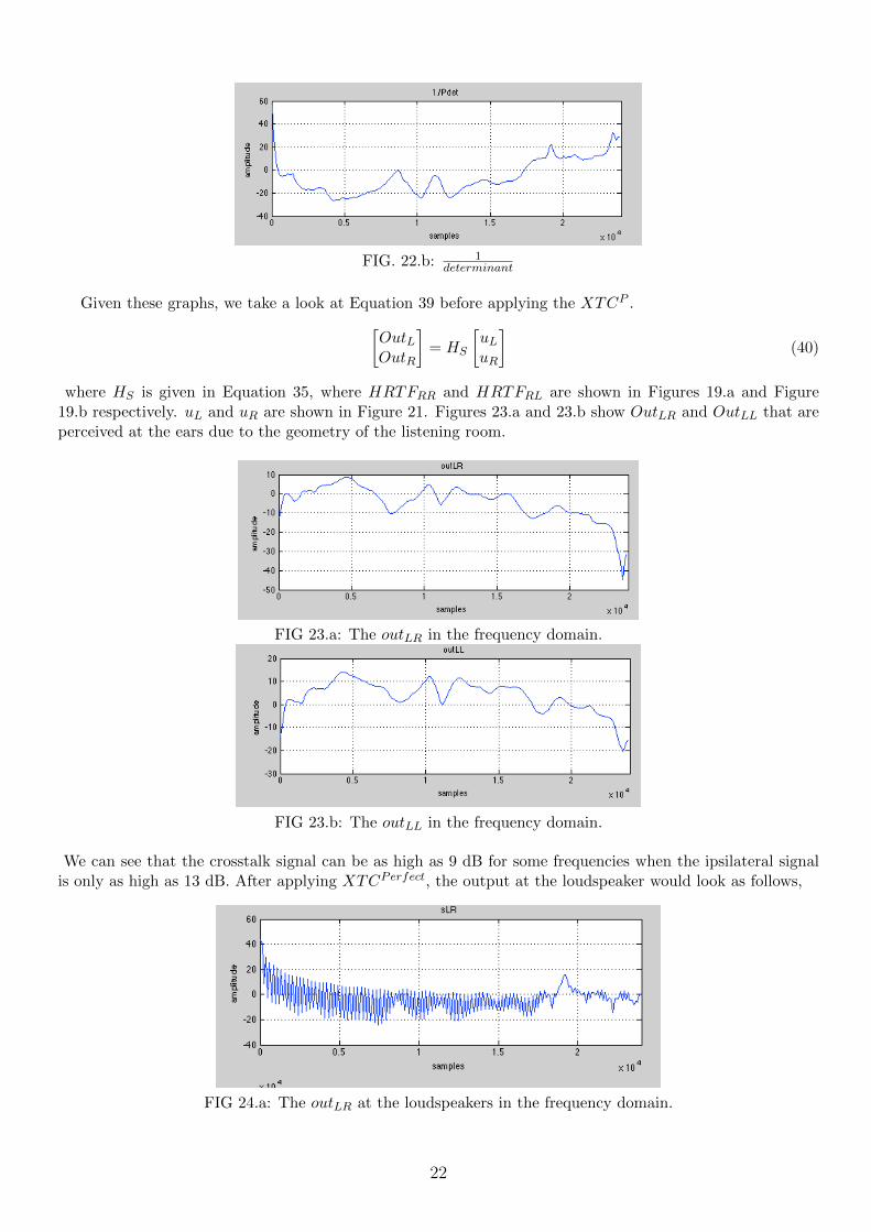
FIG. 22.b: 1determinant

Given these graphs, we take a look at Equation 39 before applying the XTCP .[OutLOutR

]= HS

[uLuR

](40)

where HS is given in Equation 35, where HRTFRR and HRTFRL are shown in Figures 19.a and Figure19.b respectively. uL and uR are shown in Figure 21. Figures 23.a and 23.b show OutLR and OutLL that areperceived at the ears due to the geometry of the listening room.

FIG 23.a: The outLR in the frequency domain.

FIG 23.b: The outLL in the frequency domain.

We can see that the crosstalk signal can be as high as 9 dB for some frequencies when the ipsilateral signalis only as high as 13 dB. After applying XTCPerfect, the output at the loudspeaker would look as follows,

FIG 24.a: The outLR at the loudspeakers in the frequency domain.

22

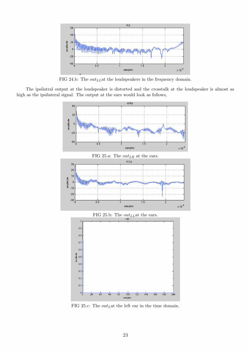
FIG 24.b: The outLLat the loudspeakers in the frequency domain.

The ipsilatral output at the loudspeaker is distorted and the crosstalk at the loudspeaker is almost ashigh as the ipsilateral signal. The output at the ears would look as follows,

FIG 25.a: The outLR at the ears.

FIG 25.b: The outLLat the ears.

FIG 25.c: The outLat the left ear in the time domain.

23

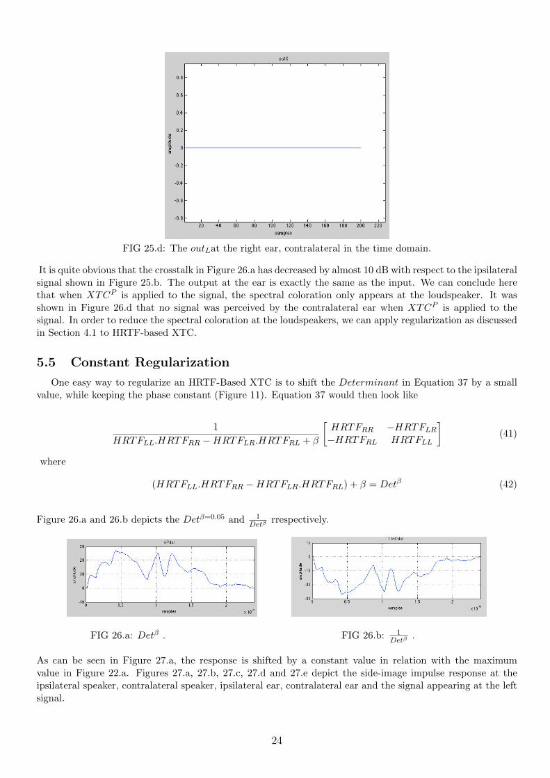
FIG 25.d: The outLat the right ear, contralateral in the time domain.

It is quite obvious that the crosstalk in Figure 26.a has decreased by almost 10 dB with respect to the ipsilateralsignal shown in Figure 25.b. The output at the ear is exactly the same as the input. We can conclude herethat when XTCP is applied to the signal, the spectral coloration only appears at the loudspeaker. It wasshown in Figure 26.d that no signal was perceived by the contralateral ear when XTCP is applied to thesignal. In order to reduce the spectral coloration at the loudspeakers, we can apply regularization as discussedin Section 4.1 to HRTF-based XTC.

5.5 Constant Regularization

One easy way to regularize an HRTF-Based XTC is to shift the Determinant in Equation 37 by a smallvalue, while keeping the phase constant (Figure 11). Equation 37 would then look like

1

HRTFLL.HRTFRR −HRTFLR.HRTFRL + β

[HRTFRR −HRTFLR−HRTFRL HRTFLL

](41)

where

(HRTFLL.HRTFRR −HRTFLR.HRTFRL) + β = Detβ (42)

Figure 26.a and 26.b depicts the Detβ=0.05 and 1Detβ

rrespectively.

FIG 26.a: Detβ . FIG 26.b: 1Detβ

.

As can be seen in Figure 27.a, the response is shifted by a constant value in relation with the maximumvalue in Figure 22.a. Figures 27.a, 27.b, 27.c, 27.d and 27.e depict the side-image impulse response at theipsilateral speaker, contralateral speaker, ipsilateral ear, contralateral ear and the signal appearing at the leftsignal.

24

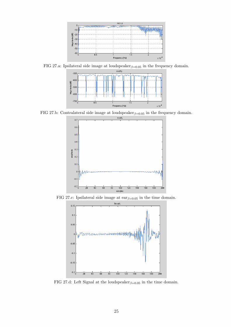
FIG 27.a: Ipsilateral side image at loudspeakerβ=0.05 in the frequency domain.

FIG 27.b: Contralateral side image at loudspeakerβ=0.05 in the frequency domain.

FIG 27.c: Ipsilateral side image at earβ=0.05 in the time domain.

FIG 27.d: Left Signal at the loudspeakerβ=0.05 in the time domain.

25

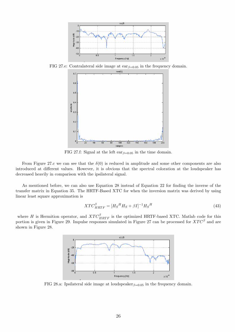
FIG 27.e: Contralateral side image at earβ=0.05 in the frequency domain.

FIG 27.f: Signal at the left earβ=0.05 in the time domain.

From Figure 27.c we can see that the δ(0) is reduced in amplitude and some other components are alsointroduced at different values. However, it is obvious that the spectral coloration at the loudspeaker hasdecreased heavily in comparison with the ipsilateral signal.

As mentioned before, we can also use Equation 28 instead of Equation 22 for finding the inverse of thetransfer matrix in Equation 35. The HRTF-Based XTC for when the inversion matrix was derived by usinglinear least square approximation is

XTCβHRTF = [HSHHS + βI]−1HS

H (43)

where H is Hermition operator, and XTCβHRTF is the optimized HRTF-based XTC. Matlab code for thisportion is given in Figure 29. Impulse responses simulated in Figure 27 can be processed for XTCβ and areshown in Figure 28.

FIG 28.a: Ipsilateral side image at loudspeakerβ=0.05 in the frequency domain.

26

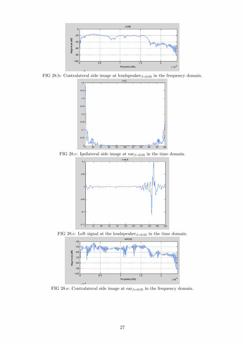
FIG 28.b: Contralateral side image at loudspeakerβ=0.05 in the frequency domain.

FIG 28.c: Ipsilateral side image at earβ=0.05 in the time domain.

FIG 28.c: Left signal at the loudspeakerβ=0.05 in the time domain.

FIG 28.e: Contralateral side image at earβ=0.05 in the frequency domain.

27

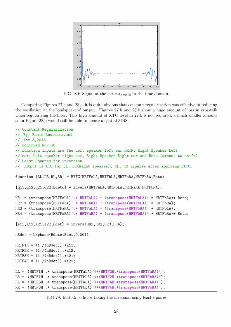
FIG 28.f: Signal at the left earβ=0.05 in the time domain.

Comparing Figures 27.c and 28.c, it is quite obvious that constant regularization was effective in reducingthe oscillation at the loudspeakers’ output. Figures 27.b and 28.b show a huge amount of loss in crosstalkwhen regularizing the filter. This high amount of XTC level in 27.b is not required; a much smaller amountas in Figure 28.b would still be able to create a spatial 3DIS.

// Constant Regularization

// By: Ramin Anushiravani

// Nov 3,2013

// modified Nov,30

// function inputs are the Left speaker left ear HRTF, Right Speaker Left

// ear, Left speaker right ear, Right Speaker Right ear and Beta (amount to shift)

// Least Squares for inversion

// Output is XTC for LL, LR(Right speaker), RL, RR impulse after applying BXTC.

function [LL,LR,RL,RR] = BXTC(HRTFaLA,HRTFbLA,HRTFaRA,HRTFbRA,Beta)

[q11,q12,q21,q22,Bdeto] = invers(HRTFaLA,HRTFbLA,HRTFaRA,HRTFbRA);

HR1 = (transpose(HRTFaLA)’.* HRTFaLA) + (transpose(HRTFbLA)’.* HRTFbLA)+ Beta;

HR2 = (transpose(HRTFaLA)’.* HRTFaRA) + (transpose(HRTFbLA)’.* HRTFbRA);

HR3 = (transpose(HRTFaRA)’.* HRTFaLA) + (transpose(HRTFbRA)’.* HRTFbLA);

HR4 = (transpose(HRTFaRA)’.* HRTFaRA) + (transpose(HRTFbRA)’.* HRTFbRA)+ Beta;

[a11,a12,a21,a22,Bdet] = invers(HR1,HR2,HR3,HR4);

nBdet = bkphase(Bdeto,Bdet,0.001);

HRTF1H = (1./(nBdet)).*a11;

HRTF2H = (1./(nBdet)).*a12;

HRTF3H = (1./(nBdet)).*a21;

HRTF4H = (1./(nBdet)).*a22;

LL = (HRTF1H .* transpose(HRTFaLA)’)+(HRTF2H.*transpose(HRTFaRA)’);

LR = (HRTF1H .* transpose(HRTFbLA)’)+(HRTF2H.*transpose(HRTFbRA)’);

RL = (HRTF3H .* transpose(HRTFaLA)’)+(HRTF4H.*transpose(HRTFaRA)’);

RR = (HRTF3H .* transpose(HRTFbLA)’)+(HRTF4H.*transpose(HRTFbRA)’);

FIG 29. Matlab code for taking the inversion using least squares.

28

In the next section, we will briefly discuss frequency dependent regularization for HRTF-based XTC .

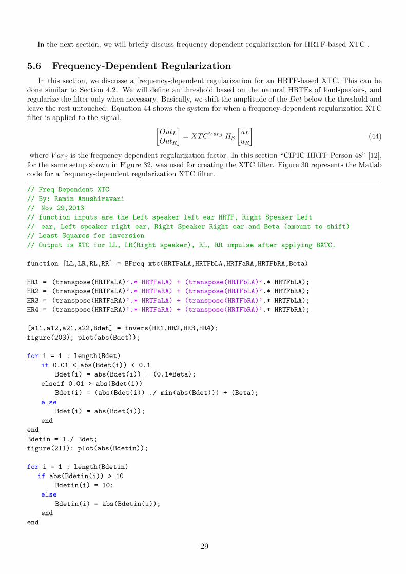
5.6 Frequency-Dependent Regularization

In this section, we discusse a frequency-dependent regularization for an HRTF-based XTC. This can bedone similar to Section 4.2. We will define an threshold based on the natural HRTFs of loudspeakers, andregularize the filter only when necessary. Basically, we shift the amplitude of the Det below the threshold andleave the rest untouched. Equation 44 shows the system for when a frequency-dependent regularization XTCfilter is applied to the signal. [

OutLOutR

]= XTCV arβ .HS

[uLuR

](44)

where V arβ is the frequency-dependent regularization factor. In this section “CIPIC HRTF Person 48” [12],for the same setup shown in Figure 32, was used for creating the XTC filter. Figure 30 represents the Matlabcode for a frequency-dependent regularization XTC filter.

// Freq Dependent XTC

// By: Ramin Anushiravani

// Nov 29,2013

// function inputs are the Left speaker left ear HRTF, Right Speaker Left

// ear, Left speaker right ear, Right Speaker Right ear and Beta (amount to shift)

// Least Squares for inversion

// Output is XTC for LL, LR(Right speaker), RL, RR impulse after applying BXTC.

function [LL,LR,RL,RR] = BFreq_xtc(HRTFaLA,HRTFbLA,HRTFaRA,HRTFbRA,Beta)

HR1 = (transpose(HRTFaLA)’.* HRTFaLA) + (transpose(HRTFbLA)’.* HRTFbLA);

HR2 = (transpose(HRTFaLA)’.* HRTFaRA) + (transpose(HRTFbLA)’.* HRTFbRA);

HR3 = (transpose(HRTFaRA)’.* HRTFaLA) + (transpose(HRTFbRA)’.* HRTFbLA);

HR4 = (transpose(HRTFaRA)’.* HRTFaRA) + (transpose(HRTFbRA)’.* HRTFbRA);

[a11,a12,a21,a22,Bdet] = invers(HR1,HR2,HR3,HR4);

figure(203); plot(abs(Bdet));

for i = 1 : length(Bdet)

if 0.01 < abs(Bdet(i)) < 0.1

Bdet(i) = abs(Bdet(i)) + (0.1*Beta);

elseif 0.01 > abs(Bdet(i))

Bdet(i) = (abs(Bdet(i)) ./ min(abs(Bdet))) + (Beta);

else

Bdet(i) = abs(Bdet(i));

end

end

Bdetin = 1./ Bdet;

figure(211); plot(abs(Bdetin));

for i = 1 : length(Bdetin)

if abs(Bdetin(i)) > 10

Bdetin(i) = 10;

else

Bdetin(i) = abs(Bdetin(i));

end

end

29

figure(202);plot(abs(Bdetin));title(’Bdetin’)

Bframe = buffer(abs(Bdetin),50);

for i = 1 : length(Bframe(1,:))

BframeW(i,:) = Bframe(:,i) .* hamming(length(Bframe(:,1));

end

BdetW = reshape(transpose(BframeW),1,length(BframeW(1,:))*length(BframeW(:,1)));

nBdet = bkphase(abs(1./Bdet),BdetW,0.005);

figure(207);plot(abs(nBdet));

figure(206); freqz(ifft(nBdet),1,200,48000);

HRTF1H = ((nBdet)).*(a11);

HRTF2H = ((nBdet)).*(a12);

HRTF3H = ((nBdet)).*(a21);

HRTF4H = ((nBdet)).*(a22);

LL = (HRTF1H .* transpose(HRTFaLA)’)+(HRTF2H.*transpose(HRTFaRA)’);

LR = (HRTF1H .* transpose(HRTFbLA)’)+(HRTF2H.*transpose(HRTFbRA)’);

RL = (HRTF3H .* transpose(HRTFaLA)’)+(HRTF4H.*transpose(HRTFaRA)’);

RR = (HRTF3H .* transpose(HRTFbLA)’)+(HRTF4H.*transpose(HRTFbRA)’);

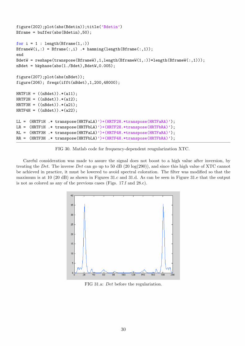
FIG 30. Matlab code for frequency-dependent reugularization XTC.

Careful consideration was made to assure the signal does not boost to a high value after inversion, bytreating the Det. The inverse Det can go up to 50 dB (20 log(290)), and since this high value of XTC cannotbe achieved in practice, it must be lowered to avoid spectral coloration. The filter was modified so that themaximum is at 10 (20 dB) as shown in Figures 31.c and 31.d. As can be seen in Figure 31.e that the outputis not as colored as any of the previous cases (Figs. 17.f and 28.c).

FIG 31.a: Det before the regulariation.

30

FIG 31.b: 1/Det before the frequency-dependent regularization.

FIG 31.c: 1/Det after the frequency-dependent regularization in samples.

FIG 31.d: 1/Det after the frequency-dependent regularization in Hz-dB.

31

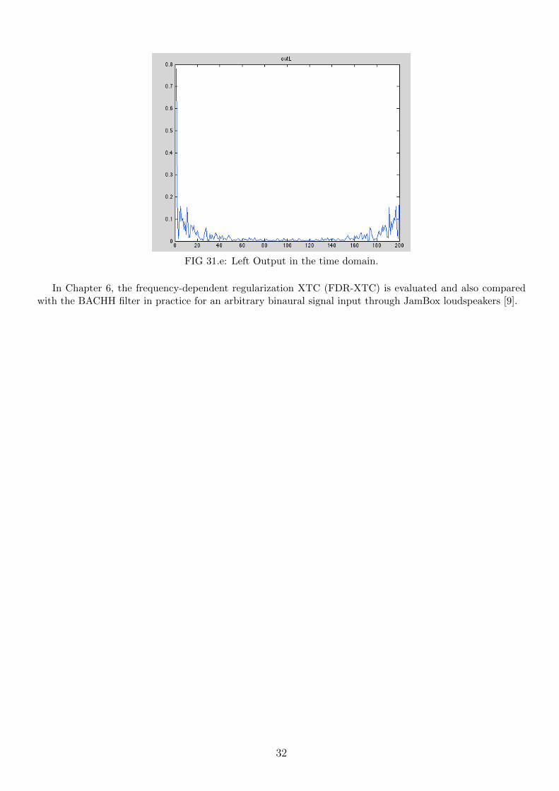
FIG 31.e: Left Output in the time domain.

In Chapter 6, the frequency-dependent regularization XTC (FDR-XTC) is evaluated and also comparedwith the BACHH filter in practice for an arbitrary binaural signal input through JamBox loudspeakers [9].

32

Chapter 6

6 Perceptual Evaluation

In this Chapter, FDR-XTC is compared with the BACCH filter in the sense of comparing an HRTF-basedXTC with the one that was created using a free-field two-point source model for an arbitrary binaural inputsignal [16].

6.1 Assumptions

In this evaluation, a few assumptions were made for the sake of fair comparison.

1. The HRTF database used in this chapter is collected from “CIPIC HRTF Person 153”. The assump-tion was made that the loudspeaker’s natural HRTF can be defined by this database, using only their angles.

2. The binaural recording signals used in this chapter were recorded for an individual in a small-officeenvironment. The assumption was made that this signal has the capability of creating the same 3D image forany other individual.

3. Another assumption made was that the difference between the HRTFs encoded into the FDR-XTC andthose into the binaural recordings are negligable.

4. The playback room is in the same recording room as where the binarual recording and speaker’s im-pulse responses were recorded, or in an anechoic chamber.

5. The listening room setup matches the one in Section 6.2.

6.2 Listening Room Setup

The listening room for the FDR-HRTF-based XTC has a specific characteristics that must be followed forbest results given the assumptions made in section 6.1. Since the BACCH filter is implemented into JamBoxloudspeakers, the FDR-HRTF-based XTC was also designed to match the characteretics of this loudspeaker,even though the actual impulse responses of the speakers were not used (first assumption).

JamBox specifications are given in [15]. It is a relatively small loudspeaker with a narrow-span stereotransducer and bluetooth capability. Figure 32 shows a regular-sized JamBox followed by Figures 33.a and33.b where the JamBox’s loudspeaker’s span were calculated for the given listening room.

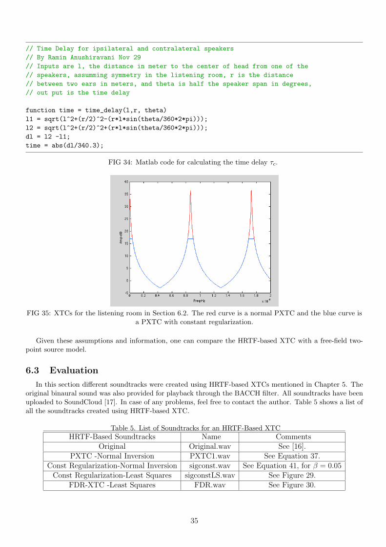
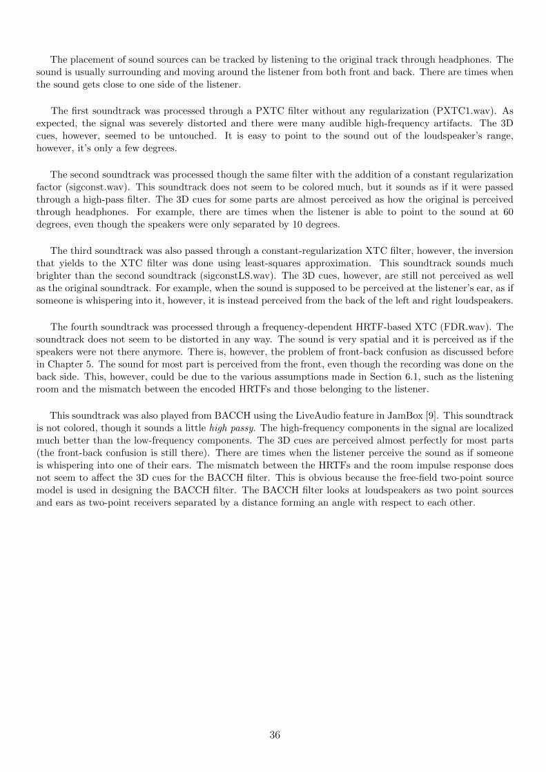
The setup is symmetric between the listener’s left and right sides. The ipsilateral length, L1, is about 0.59m. The contralateral length, L2, is about 0.61 m. The loudspeaker’s span turn out to be about 10 degrees(Figure 33.b). Therefore, the HRTFs used for creating the XTC filter, loudspeaker’s natural HRTFs, are at -5and +5 degrees. This setup causes a time Delay, τc , between the ipsilateral and the contralateral ear of about57.8 us. The Matlab code for calculating the time delay is given in Figure 34. If we evaluate the PXTC filterfor this setup as was done earlier in Figure 12, then we can see that the high-frequency boosts are shifted moretowards 20 kHz. This could mean that the XTC filter has an advantage due to the choice of the loudspeakerfor this setup. This is shown in Figure 35, where the red curve is a non-regularized PXTC and the blue curverepresents a PXTC with constant regularization.

33

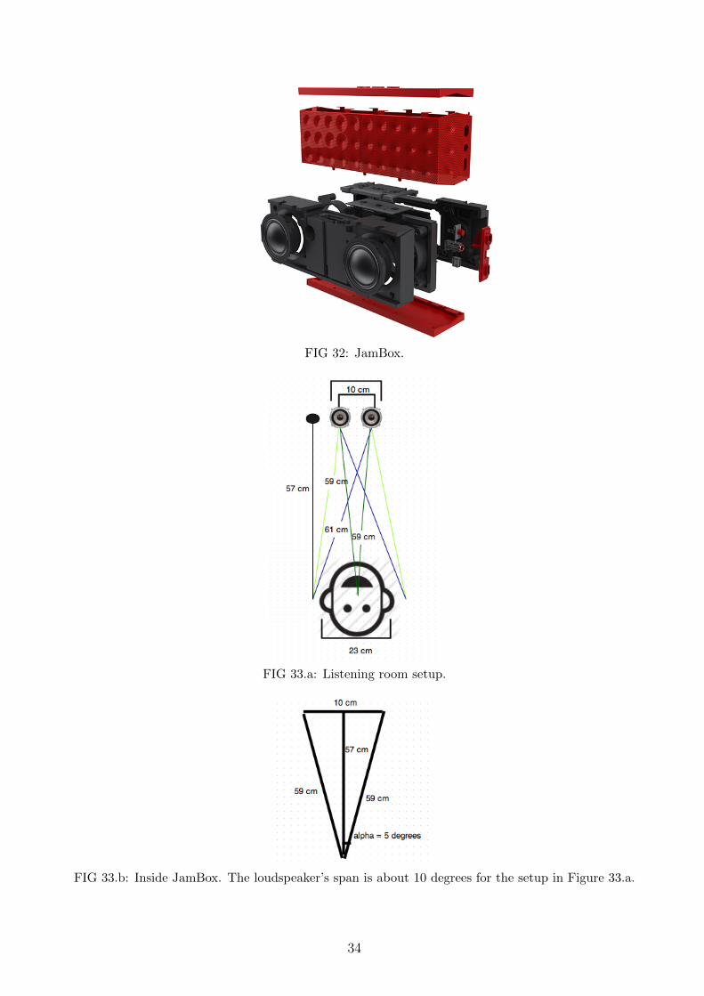
FIG 32: JamBox.

FIG 33.a: Listening room setup.

FIG 33.b: Inside JamBox. The loudspeaker’s span is about 10 degrees for the setup in Figure 33.a.

34

// Time Delay for ipsilateral and contralateral speakers

// By Ramin Anushiravani Nov 29

// Inputs are l, the distance in meter to the center of head from one of the

// speakers, assumming symmetry in the listening room, r is the distance

// between two ears in meters, and theta is half the speaker span in degrees,

// out put is the time delay

function time = time_delay(l,r, theta)

l1 = sqrt(l^2+(r/2)^2-(r*l*sin(theta/360*2*pi)));

l2 = sqrt(l^2+(r/2)^2+(r*l*sin(theta/360*2*pi)));

dl = l2 -l1;

time = abs(dl/340.3);

FIG 34: Matlab code for calculating the time delay τc.

FIG 35: XTCs for the listening room in Section 6.2. The red curve is a normal PXTC and the blue curve isa PXTC with constant regularization.

Given these assumptions and information, one can compare the HRTF-based XTC with a free-field two-point source model.

6.3 Evaluation

In this section different soundtracks were created using HRTF-based XTCs mentioned in Chapter 5. Theoriginal binaural sound was also provided for playback through the BACCH filter. All soundtracks have beenuploaded to SoundCloud [17]. In case of any problems, feel free to contact the author. Table 5 shows a list ofall the soundtracks created using HRTF-based XTC.

Table 5. List of Soundtracks for an HRTF-Based XTCHRTF-Based Soundtracks Name Comments

Original Original.wav See [16].PXTC -Normal Inversion PXTC1.wav See Equation 37.

Const Regularization-Normal Inversion sigconst.wav See Equation 41, for β = 0.05Const Regularization-Least Squares sigconstLS.wav See Figure 29.

FDR-XTC -Least Squares FDR.wav See Figure 30.

35

The placement of sound sources can be tracked by listening to the original track through headphones. Thesound is usually surrounding and moving around the listener from both front and back. There are times whenthe sound gets close to one side of the listener.

The first soundtrack was processed through a PXTC filter without any regularization (PXTC1.wav). Asexpected, the signal was severely distorted and there were many audible high-frequency artifacts. The 3Dcues, however, seemed to be untouched. It is easy to point to the sound out of the loudspeaker’s range,however, it’s only a few degrees.

The second soundtrack was processed though the same filter with the addition of a constant regularizationfactor (sigconst.wav). This soundtrack does not seem to be colored much, but it sounds as if it were passedthrough a high-pass filter. The 3D cues for some parts are almost perceived as how the original is perceivedthrough headphones. For example, there are times when the listener is able to point to the sound at 60degrees, even though the speakers were only separated by 10 degrees.

The third soundtrack was also passed through a constant-regularization XTC filter, however, the inversionthat yields to the XTC filter was done using least-squares approximation. This soundtrack sounds muchbrighter than the second soundtrack (sigconstLS.wav). The 3D cues, however, are still not perceived as wellas the original soundtrack. For example, when the sound is supposed to be perceived at the listener’s ear, as ifsomeone is whispering into it, however, it is instead perceived from the back of the left and right loudspeakers.

The fourth soundtrack was processed through a frequency-dependent HRTF-based XTC (FDR.wav). Thesoundtrack does not seem to be distorted in any way. The sound is very spatial and it is perceived as if thespeakers were not there anymore. There is, however, the problem of front-back confusion as discussed beforein Chapter 5. The sound for most part is perceived from the front, even though the recording was done on theback side. This, however, could be due to the various assumptions made in Section 6.1, such as the listeningroom and the mismatch between the encoded HRTFs and those belonging to the listener.

This soundtrack was also played from BACCH using the LiveAudio feature in JamBox [9]. This soundtrackis not colored, though it sounds a little high passy. The high-frequency components in the signal are localizedmuch better than the low-frequency components. The 3D cues are perceived almost perfectly for most parts(the front-back confusion is still there). There are times when the listener perceive the sound as if someoneis whispering into one of their ears. The mismatch between the HRTFs and the room impulse response doesnot seem to affect the 3D cues for the BACCH filter. This is obvious because the free-field two-point sourcemodel is used in designing the BACCH filter. The BACCH filter looks at loudspeakers as two point sourcesand ears as two-point receivers separated by a distance forming an angle with respect to each other.

36

Chapter 7

7 Conclusion

In this chapter, both BACCH and HRTF-based XTC filters are summarized and compared. We alsodiscussed some possible improvments to both systems in Section 7.2.

7.1 Summary

In summary, we discussed the 3D audio playback through two loudspeakers. The main challenge withplayback through loudspeakers was crosstalk. Crosstalk occurs because the 3D cues encoded into left and rightsignals are also percieved by the contralateral ear. It was discussed further that crosstalk can be eliminatedusing digital crosstalk cancellation filters. Three major previous XTC filters were discussed, Microsoft Personal3D Audio, OSD and BACCH filters.

The most successful XTC was BACCH, which used a free-field two-point source model. Since BACCHdoes not take spectral cues into consideration, it works best for most people in most environments. We alsodiscussed HRTF-based XTC in comparison with BACCH filter. HRTF-based XTC takes an individual soundlocalization system into consideration. HRTF-based XTC would sound better than the BACCH filter since itcontains spectral cues in addition to ITD and ILD. However, HRTF-based XTC has to be played back underprecise measurements and it works best for an individual whose HRTFs were encoded into the filter.

In both cases, there are some constraints to designing the filter. In a perfect case (PXTC), the inversionof the transfer matrix is applied to input signals. In BACCH, the inversion matrix elements are constructedusing acoustic wave equations and in HRTF-based XTC, they are measured for an individual in the room.PXTC, however, adds severe spectral coloration to the signal and must be regularized in advance and afterinversion. We discussed two main methods to regularize an XTC filter, constant regularization and frequencydependent regularization.

Constant regularization can reduce the coloration at the cost of losing some XTC. It does, however,introduce low-frequency rolloffs and high-frequency artifacts to the sound. This can be prevented using afrequency-dependent regularization (FDR). FDR regularizes the filter by defining a threshold; the signal isregularized above that threshold and left untouched below that level.

Overall, we can conclude that FDR regularization XTC is the best solution to regularizing an XTC filter.A free-field two-point source model would make a better entertainment system due to its simplicity and thefact that it is not individualized to one person. Both methods, however, are only designed for a limited sweetspot. This is discussed furthre in the next section.

7.2 Future Work

It is known that the listener’s head movement can severely distort the signal perceived at the listener’sears as shown in Figure 7. This can be improved by creating a real-time sweet spot as done in [6, 18, 21].For example, in the case of a BACCH filter one can use a Kinect depth camera to track an individual’s headand measure the ipsilateral and contralateral distances to create new XTC filters in real-time. We can alsoincorporates user interface into the system. For example, a recording headset can be provided to the user. Thesystem can then be calibrated using HRTF-based XTC, by extracting the impulse responses at the listener’sear in real time. There are also ways to design more sophisticated models for creating an adaptive BACCHfilter. For example, one can also model the room impulse response [19] and also the ear frequency response[20] when using the free field two-point source model.

37

References

[1] Zea, E. Binaural in-ear monitoring of acoustic instruments in live music performance (2012) 15thInternational Conference on Digital Audio Effects, DAFx 2012 Proceedings, 8 p.

[2] “HRTF Measurements of a KEMAR Dummy-Head Microphone.” HRTF Measurements of a KEMARDummy-Head Microphone. Web. 01 Dec. 2013.[Online]. Available:http://sound.media.mit.edu/resources/KEMAR.html

[3] “Sound Localization.” Monaural and Binaural Cues for A I Thzmu and El Tievaon, 25 Feb. 2011.[Online]. Available:http://www.bcs.rochester.edu/courses/crsinf/221/ARCHIVES/S11/Localization1.pdf

[4] “Sound Localization and the Auditory Sce Ne.” Washington University.[Online]. Available:http://courses.washington.edu/psy333/lecture_pdfs/Week9_Day2.pdf

[5] E. Choueiri, “Optimal Crosstalk Cancellation for Binaural Audio with Two Loudspeakers,” PrincetonUniversity. [Online]. Available: http://www.princeton.edu/3D3A/Publications/BACCHPaperV4d.pdf.

[6] M. Song, C. Zhang, D. Florencio, “Personal 3D Audio System with Loudspeakers,” IEEE 2010.

[7] “Virtual Acoustics and Audio Engineering: Optimal Source Distribution.” Virtual Acoustics and AudioEngineering: Optimal Source Distribution. Web. 01 Dec. 2013. [Online]. Available:http://resource.isvr.soton.ac.uk/FDAG/VAP/html/osd.html

[8] Takeuchi T, Nelson PA. “Engineering and the Environment, University of Southampton.” OptimalSource Distribution. Web. 01 Dec. 2013.

[9] Jambox, “Software Update 2.1”, [Online]. Available: https://jawbone.com/liveaudio, JawboneJambox.

[10] Sang-Jin Cho; Ovcharenko, A.; Ui-Pil Chong, “Front-Back Confusion Resolution in 3D SoundLocalization with HRTF Databases,” Strategic Technology, The 1st International Forum on, pp. 239, 243,18-20 Oct. 2006.

[11] “Extracting the System Impulse Response from MLS Measurement.” Extracting the System ImpulseResponse from MLS Measurement. Web. 01 Dec. 2013. [Online]. Available:http://www.kempacoustics.com/thesis/node85.html

[12] “CIPIC International Laboratory.” CIPIC International Laboratory. Web. 01 Dec. 2013. [Online].Available: http://interface.cipic.ucdavis.edu/sound/hrtf.htm

[13] 3D3A Lab at Princeton University. Web. 01 Dec. 2013. [Online]. Available:http://www.princeton.edu/3D3A/PureStereo/Pure_Stereo.html

[14] Kinsler, Lawrence E., and Austin R. Frey. Fundamentals of Acoustics. New York: Wiley, 1962. Print.

[15] “Jambox The Remix.” Jawbone.com. 01 Dec. 2013. [Online]. Available:https://jawbone.com/speakers/jambox/specs

38

[16] Anushiravani, Ramin. “Joker Interrogation Scene (3D Audio for Headphone).” Web. YouTube. 03Aug. 2013. 01 Dec. 2013. [Online]. Available: http://www.youtube.com/watch?v=x_kwi0yaH5w

[17] “3D Audio Playback Through Two Loudspeakers.” SoundCloud. 01 Dec. 2013. [Online]. Available:https://soundcloud.com/ramin-anushir/sets/3d-audio-playback-through-two

[18] Javier Lpez, Jos, and Alberto Gonzlez. “3-D Audio With Video Tracking For MultimediaEnvironments.” Journal Of New Music Research 30.3 (2001): 271. Academic Search Premier. Web. 1 Dec.2013.

[19] “Room Impulse Response Data Set — Isophonics.” Room Impulse Response Data Set — Isophonics.Web. 01 Dec. 2013.[Online]. Available:http://isophonics.net/content/room-impulse-response-data-set

[20] “Frequency Response of the Ear.” Fsear. Web. 01 Dec. 2013.[Online]. Available:http://www.engr.uky.edu/~donohue/audio/fsear.html

[21] Peter Lessing, “A Binaural 3D Sound System Applied to Moving Sources,” Institute of ElectronicMusic and Acoustics (IEM). University of Music and Dramatic Arts of Graz, Master Thesis. [Online].Available: http://iem.kug.ac.at/fileadmin/media/iem/altdaten/projekte/acoustics/awt/binaural/binaural.pdf

39

Appendix

Matlab Codes

In this appendix you can find the Matlab code for simulating the frequency response of the BACCH XTCfilter (e.g., the Matlab code for calculating the ill-conditioned frequency indices).

//Perfect XTC, Constant Regularization XTC, Adaptive Regularization

// By Ramin Anushiravani Oct/12/13

// Modified Oct/13

td = time_delay(0.59,0.23,5)

// P-XTC

tc= td;

g = 0.985;

f = 1:10:20000;

w = f.* 2*pi;

Si = 1./(sqrt(g^4-(2*g^2*cos(2*w*tc))+1));

Sci = 1./(2*(sqrt(g^2+(2*g*cos(w*tc))+1)));

Sphase = max(1./(sqrt(g^2+(2*g*cos(w*tc))+1)),1./(sqrt(g^2-(2*g*cos(w*tc))+1)));

beta = 0.05;

gamma = 20*log10(1/(2*sqrt(beta)));

plot(f,(20.*log10(Sphase)),’r’);xlabel(’Freq-Hz’);ylabel(’Amp-dB’);

for i = 1 : length(Sphase)

if (Sphase(i)) > gamma

Sphase(i) = gamma;

else

Sphase(i) = Sphase(i);

end

end

hold on; plot(f,(20.*log10(Sphase)),’b’);xlabel(’Freq-Hz’);ylabel(’Amp-dB’);

// peaks for which we need to boost the signal

// Side Image Ipisilatteral

// npi

SsiIImax = 20*log10(1/(1-g^2)) //amount to be shifted in dB

n = 0 : 1 : 8;

w = (n * pi)/tc;

fsiIImax = w./(2*pi) //freq needs to be boosted for side image ipsilatereal

//npi/2

n = 1 : 2 :9

SsiImin = 20*log10(1/(1+g^2)) // amount to attenuated

w = (n * pi/2)/tc;

fsiImin = w./(2*pi) // frequecies to be attenuated

// Side Image CrossTalk

//npi

SsiXmax = 20*log10(g/(1-g^2))

// Same frequncies

// npi/2

40

SsiXmin = 20*log10(g/(1+g^2))

//Center Image

// npi

n = 1 : 2 :9

Scemax = 20*log10(1/(2-(2*g)))

w = (n * pi)/tc;

fceMax = w./(2*pi)

// npi/

n = 0 : 2 :10

Scemin = 20*log10(1/(2+(2*g)))

w = (n * pi)/tc;

fceMin = w./(2*pi)

// Metric Phase.

// npi

n = 1 : 1 :9;

Sphmax = 20*log10(1/(1-g))

w = (n * pi)/tc;

fphMax = w./(2*pi)

// npi/2

n = 1 : 1 :9;

Sphmax = 20*log10(1/sqrt(1+g^2))

w = (n * pi/2)/tc;

fphMin = w./(2*pi)

//Calculating tc from l and speaker span

l = 1.6 //distance from speakers to the middle of the head m

dr = 0.15 //distance between ears m

theta = (18/180) * pi //speaker span raidan VERY VERY Important the smaller the smaller

tc, less peaks in freq response less //spectral coloration in hearing range

l1 = sqrt(l^2+(dr/2)^2-(dr*l*sin(theta/2)));

l2 = sqrt(l^2+(dr/2)^2+(dr*l*sin(theta/2)));

g = l1 / l2; // distance ratio less than 1 between ipsilateral and contralateral

cs = 340.3;

dl = abs(l2 - l1);

tc = dl/cs;

// Condition number

c= 65*10^-6;

g = 0.985;

f = 1:10:22000;

w = f.* 2*pi;

kc =

max(sqrt(2*(g^2+1)./(g^2+2*g*cos(w*tc)+1)-1),sqrt(2*(g^2+1)./(g^2-2*g*cos(w*tc)+1)-1));

figure(3);plot(f,kc) //where it’s ill-conditioned

// shifting

n = 0:1:5;

k = (1+g)/(1-g) //condition number value at higher freq

w = (n * pi)/tc;

fill_Condition = w./(2*pi) //those frequencies of - illconditioned

n = 1:2:9;

w = (n * pi/2)/tc; //k is zero, no need for boost

fwell_Condition = w./(2*pi)

41

// B-XTC Const B

//Spectral Envelope

tc= 65*10^-6;

g = 0.985;

f = 1:10:20000;

w = f.* 2*pi;

B = 0;

S = max(sqrt(g^2+(2*g*cos(w*tc))+1)./(g^2+(2*g*cos(w*tc))+B+1),

sqrt(g^2-2*g*cos(w*tc)+1)./(g^2-(2*g*cos(w*tc))+B+1) );

figure(33);plot(f,(20.*log10(S)));xlabel(’Freq-Hz’);ylabel(’Amp-dB’);hold on;

B = 0.05;

S = max(sqrt(g^2+(2*g*cos(w*tc))+1)./(g^2+(2*g*cos(w*tc))+B+1),

sqrt(g^2-2*g*cos(w*tc)+1)./(g^2-(2*g*cos(w*tc))+B+1) );

plot(f,(20.*log10(S)),’r’);xlabel(’Freq-Hz’);ylabel(’Amp-dB’);hold on;

B = 0.005;

S = max(sqrt(g^2+(2*g*cos(w*tc))+1)./(g^2+(2*g*cos(w*tc))+B+1),

sqrt(g^2-2*g*cos(w*tc)+1)./(g^2-(2*g*cos(w*tc))+B+1) );

plot(f,(20.*log10(S)),’g’);xlabel(’Freq-Hz’);ylabel(’Amp-dB’); title(’B=XTC , B=0 r,

B=0.05 r, B=0.005 g’);

// doublet peaks and singlet peaks attenuation

B = 0.0001;

Bs = 20*log10(B/((g-1)^2+1)) //singlet peaks -> Perfect XTC

B = 0.05;

Bb1 = 20*log10(2*sqrt(B)/(1-g)) // doublet peaks attenuation

B = 0.005

Bb2 = 20*log10(2*sqrt(B)/(1-g))

// Freq respons for const reg at ear

tc= 65*10^-6; //19*10^-6;//2 * 10^-4 ; //65*10^-6; //Depends only on the set up!

g = 0.985;

f = 1:10:20000;

w = f.* 2*pi;

B = 0.005;

X = (g^4 + (B * g^2) - (2*(g^2)*cos(2*w*tc))+B+1)./(2*g*B*abs(cos(w*tc))); //XTC

performance

figure;plot(f,20.*log10(X));axis([0 21000 -10 40])

B = 0.05;

X = (g^4 + (B * g^2) - (2*(g^2)*cos(2*w*tc))+B+1)./(2*g*B*abs(cos(w*tc))); //XTC

performance

hold on;plot(f,20.*log10(X),’r’);axis([0 20000 -10 90]);xlabel(’freq hz’);ylabel(’amp

-dB’);

B = 0.005;

Esii = (g^4 + (B * g^2) -

(2*(g^2)*cos(2*w*tc))+B+1)./(-2*g^2*(cos(2*w*tc))+(g^2+B)^2+2*B+1);

plot(f,20*log10(Esii));

B = 0.05;

Esii = (g^4 + (B * g^2) -

42

(2*(g^2)*cos(2*w*tc))+B+1)./(-2*g^2*(cos(2*w*tc))+(g^2+B)^2+2*B+1);

hold on;plot(f,20*log10(Esii),’r’);title(’Performance XTC 0.005 b, 0.05 r/ ESii small

one’);

// Impulse Response HLL, HLR...

tc= 65*10^-6;/

f = 0:3:20000; //20k/increament = number of samples

g = 0.985;

w = f* 2*pi;

B = 0.05;

HLL = ((exp(4*1i*w*tc)*g^2) -

((B+1)*exp(1i*2*w*tc)))./(g^2.*exp(1i*4*w*tc)+g^2-((g^2+B)^2+2*B+1));

HLR = ((exp(1i*w*tc)*g) -

(g*(g^2+B)*exp(1i*3*w*tc)))./(g^2.*exp(1i*4*w*tc)+g^2-((g^2+B)^2+2*B+1));

figure;plot(f,20*log10(abs(HLL)));

hold on; plot(f,20*log10(abs(HLR)),’r’);title(’HRTF ipsilatteral b, HRTF contralateral

XT r’);xlabel(’freq hz’);ylabel(’amp-db’)

hll = ifft(HLL);

hlr = ifft(HLR);

Max1 = max(abs(hll));

Max2 = max(abs(hlr));

Max = max(Max1,Max2);

figure;stem(((hll)/Max));hold on; stem(((hlr)/Max),’r’);title(’hlr r, hll

b’);xlabel(’sample’);ylabel(’amp’);

43