3d computer vision: csc 83020. instructor: ioannis stamos istamos (at) hunter.cuny.edu ioannis...
TRANSCRIPT
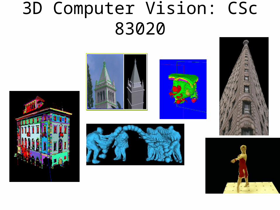
3D Computer Vision: CSc 83020
Instructor: Ioannis Stamosistamos (at) hunter.cuny.edu
http://www.cs.hunter.cuny.edu/~ioannis
Office Hours: Tuesdays 4-6 (at Hunter) or by appoitnment
Office: 1090G Hunter North (69th street bw. Park and Lex.)
Computer Vision Lab: 1090E Hunter North
Course web page: http://www.cs.hunter.cuny.edu/~ioannis/3D_f12.html
3D Computer Vision: CSc 83020
Goals
• To familiarize you with basic the techniques and jargon in the field
• To enable you to solve computer vision problems
• To let you experience (and appreciate!) the difficulties of real-world computer vision
• To get you excited!

Class Policy
• You have to– Turn in all assignments (60% of grade)– Complete a final project (30% of grade)– Actively participate in class (10% of grade)
• Late policy– Six late days (but not for final project)
• Teaming– For final project you can work in groups of 2
About me
• 11th year at Hunter and the Graduate Center
• Graduated from Columbia in ’01– CS Ph.D.
• Research Areas:– Computer Vision– 3D Modeling– Computer Graphics
BooksComputer Vision: Algorithms and Applications, Richard Szeliski, 2010 (available
online for free)Robot Vision B. K. P. Horn, The MIT Press (great classic book)Introductory Techniques for 3-D Computer Vision Emanuele Trucco and Alessandro Verri, Prentice Hall, 1998 (algorithmic
perspective)Computer Vision A Modern ApproachDavid A. Forsyth, Jean Ponce, Prentice Hall 2003An Invitation to 3-D Vision Yi Ma, Stefano Soatto, Jana Kosecka, S. Shankar Sastry
Springer 2004.Three-Dimensional Computer Vision: A Geometric Viewpoint Olivier Faugeras The MIT Press, 1996.
Journals/Web• International Journal of Computer Vision.• Computer Vision and Image Understanding.• IEEE Trans. on Pattern Analysis and Machine Intelligence.• SIGGRAPH (mostly Graphics)• http://www.ri.cmu.edu/ (CMU’s Robotic Institute)• http://www.cs.cmu.edu/~cil/vision.html (The Vision Home Page)• http://www.dai.ed.ac.uk/CVonline/ (CV Online)• http://iris.usc.edu/Vision-Notes/bibliography/contents.html (Annotated CV Bibliography)
Class History
• Based on class taught at Columbia University
by Prof. Shree Nayar.• New material reflects modern approach.• Taught similar class at Hunter • Taught “3D Photography” class at the Graduate Center of
CUNY.• My active research area
– Funded by the National Science Foundation

Class Schedule
• Check class website
• Final project proposals– Due Nov. 7– Design your own or check list of possible
projects on class website
• Final project presentations and report– May 16 (last class)
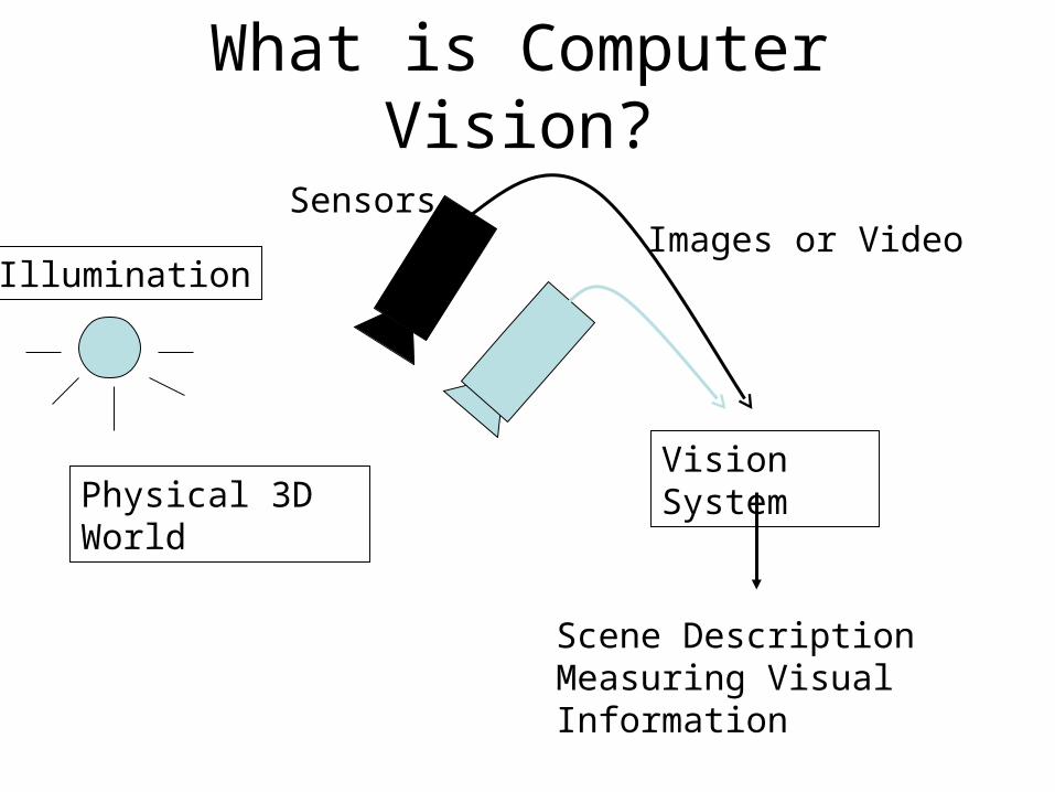
What is Computer Vision?
Physical 3D World
Illumination
Vision System
Scene DescriptionMeasuring Visual Information
SensorsImages or Video
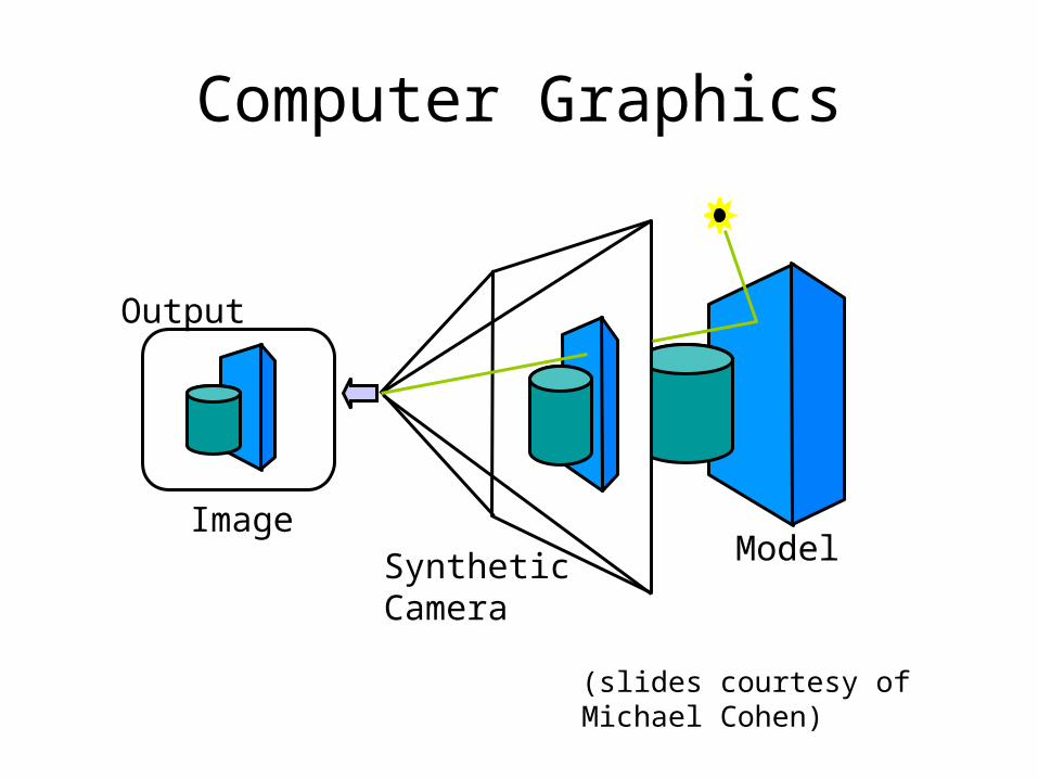
Computer Graphics
Image
Output
ModelSyntheticCamera
(slides courtesy of Michael Cohen)

Real Scene
Computer Vision
Real Cameras
Model
Output
(slides courtesy of Michael Cohen)
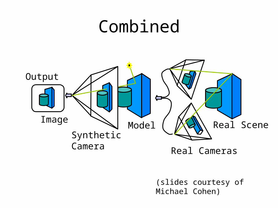
Combined
Model Real Scene
Real Cameras
Image
Output
SyntheticCamera
(slides courtesy of Michael Cohen)
Cont.
• Vision is automating visual processes (Ball & Brown).• Vision is an information processing task (Marr).• Vision is inverting image formation (Horn).• Vision is inverse graphics.• Vision looks easy, but is difficult.• Vision is difficult, but it is fun (Kanade).• Vision is useful.
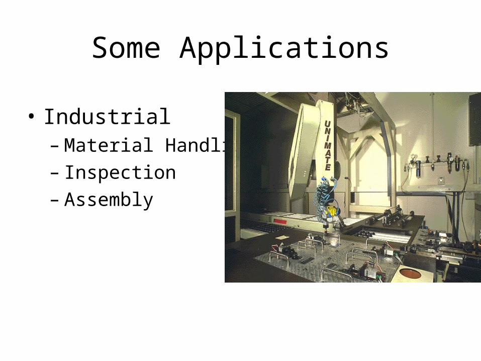
Some Applications
• Industrial – Material Handling– Inspection– Assembly
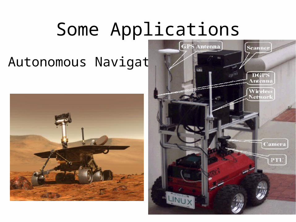
Some Applications
Autonomous Navigation
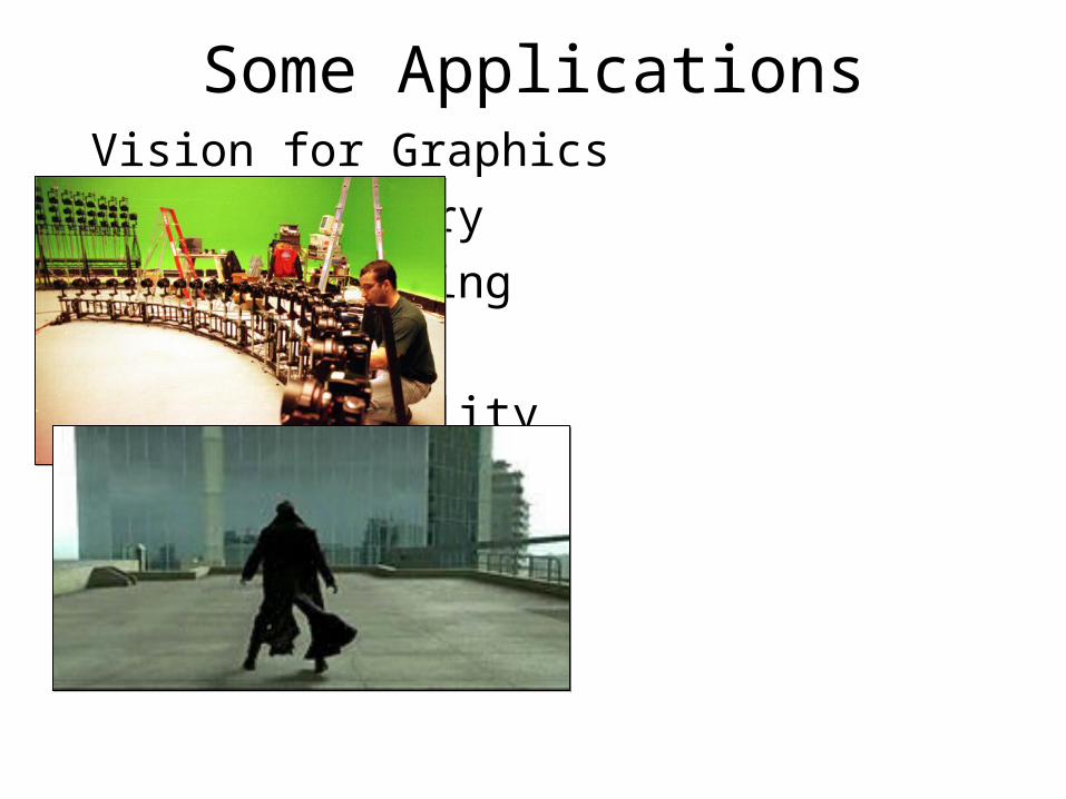
Vision for Graphics
Film Industry
Urban Planning
E-commerce
Virtual Reality
Some Applications
Some Applications
• Realistic 3D experience– Google Earth
http://earth.google.com/– Microsoft Photosynth
http://labs.live.com/photosynth/
More Applications!
• Optical Character Recognition (OCR)
• Visual Databases (images or movies)– Searching for image content
• Face Recognition (security)
• Iris Recognition (security)
• Traffic Monitoring Systems
• Many more…
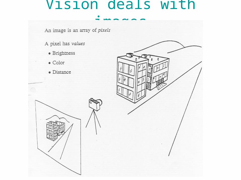
Vision deals with images

Images Look Nice…

Ioannis Stamos – CSc 83020 Spring 2007
Images Look Nice…
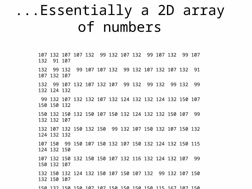
...Essentially a 2D array of numbers
107 132 107 107 132 99 132 107 132 99 107 132 99 107 132 91 107
132 99 132 99 107 107 132 99 132 107 132 107 132 91 107 132 107
132 99 107 132 107 132 107 99 132 99 132 99 132 99 132 124 132
99 132 107 132 132 107 132 124 132 132 124 132 150 107 150 150 132
150 132 150 132 150 107 150 132 124 132 132 150 107 99 132 132 107
132 107 132 150 132 150 99 132 107 150 132 107 150 132 124 132 132
107 150 99 150 107 150 132 107 150 132 124 132 150 115 124 132 150
107 132 150 132 150 150 107 132 116 132 124 132 107 99 150 132 107
132 150 132 124 132 150 107 150 107 132 99 132 107 150 132 150 107
150 132 150 150 107 107 150 150 150 150 115 167 107 150 107 132 150
107 150 132 124 132 124 132 124 132 124 132 150 107 150 107 107 132
116 132 150 132 150 107 150 150 132 150 132 116 132 124 132 150 132
150 150 150 132 116 132 116 107 132 99 150 150 132 107 132 150 107
150 132 124 132 116 132 107 150 132 107 150 132 150 107 150 107 132
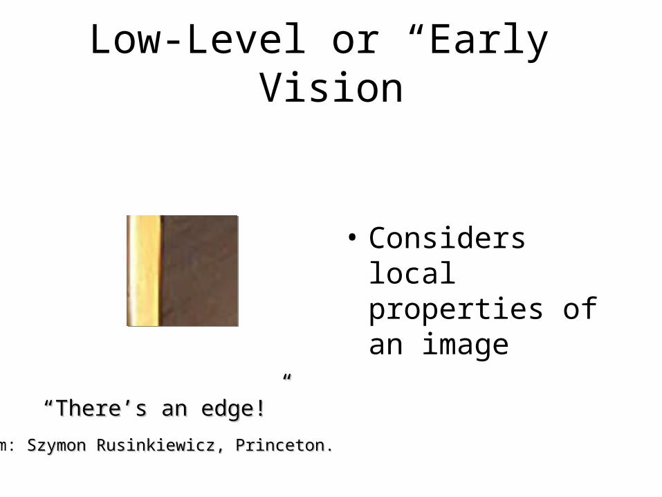
Low-Level or “Early” Vision
• Considers local properties of an image
““There’s an edge!”There’s an edge!”
From: Szymon Rusinkiewicz, Princeton.Szymon Rusinkiewicz, Princeton.
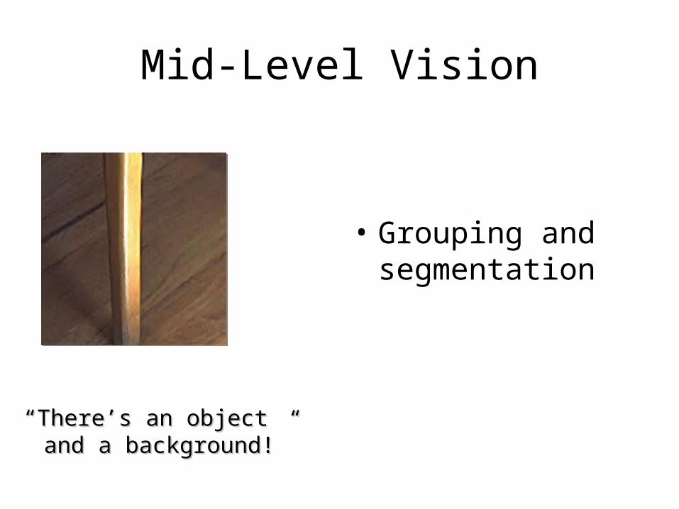
Mid-Level Vision
• Grouping and segmentation
““There’s an object There’s an object and a background!”and a background!”
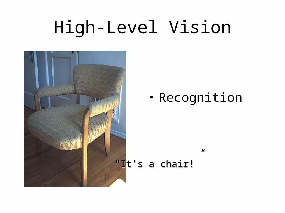
High-Level Vision
• Recognition
““It’s a chair!”It’s a chair!”
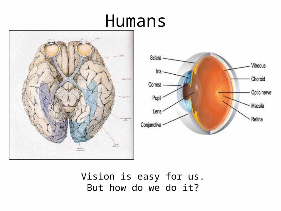
Humans
Vision is easy for us.But how do we do it?
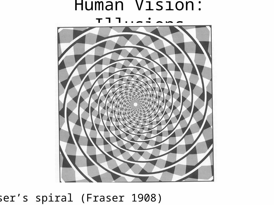
Human Vision: Illusions
Fraser’s spiral (Fraser 1908)
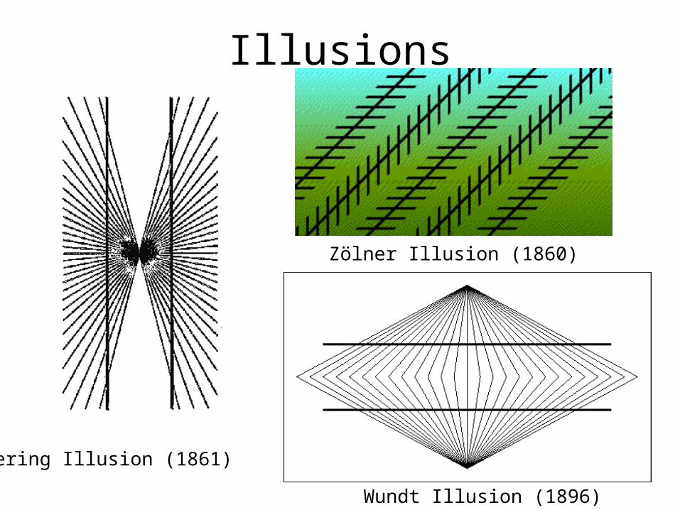
Illusions
Hering Illusion (1861)
Wundt Illusion (1896)
Zölner Illusion (1860)
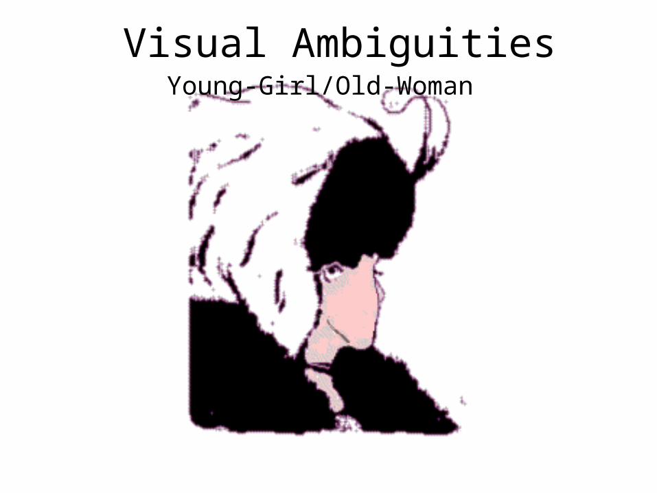
Visual AmbiguitiesYoung-Girl/Old-Woman
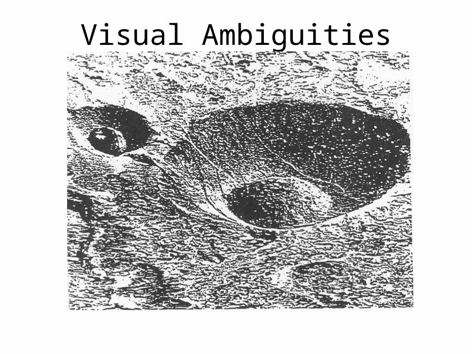
Visual Ambiguities
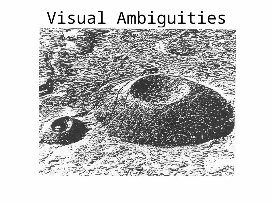
Visual Ambiguities
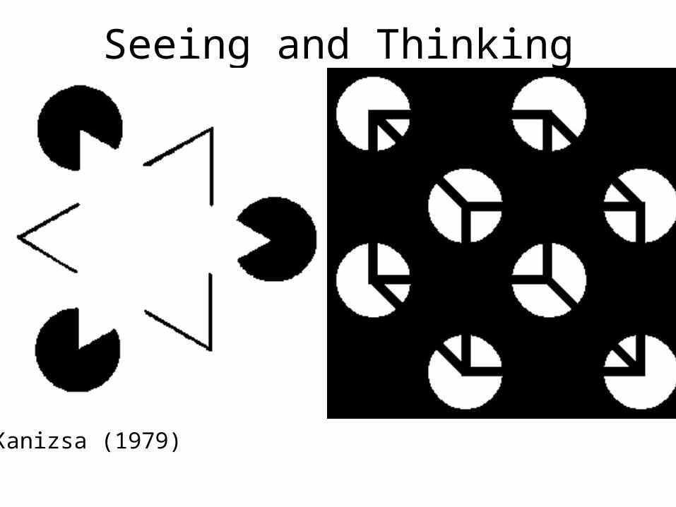
Seeing and Thinking
Kanizsa (1979)

Syllabus Overview
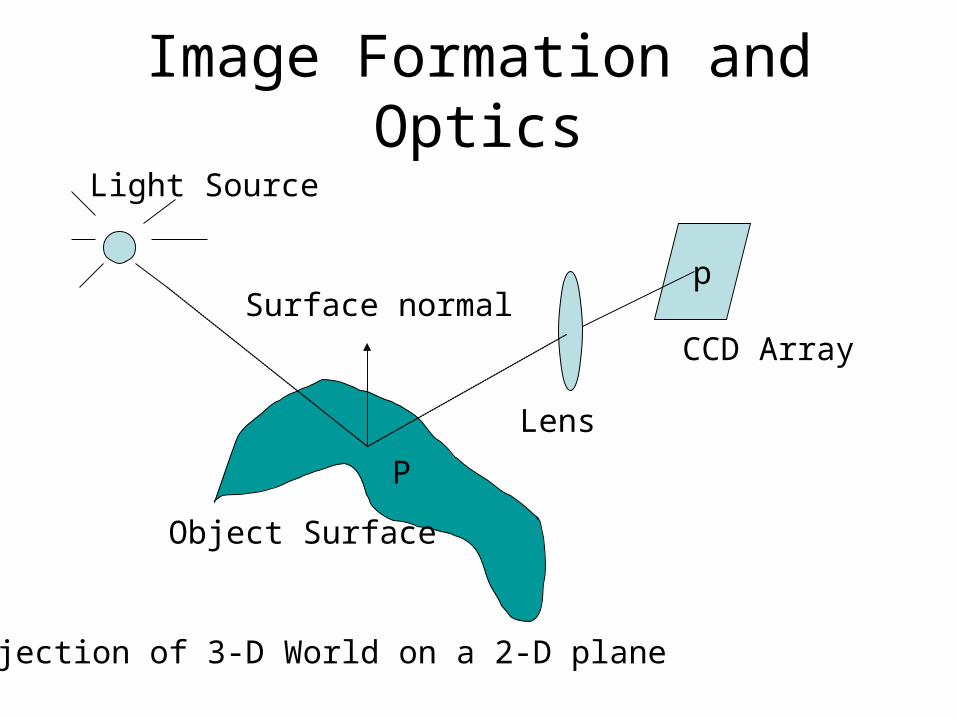
Image Formation and Optics
p
Light Source
Object Surface
Lens
CCD Array
P
Surface normal
Projection of 3-D World on a 2-D plane
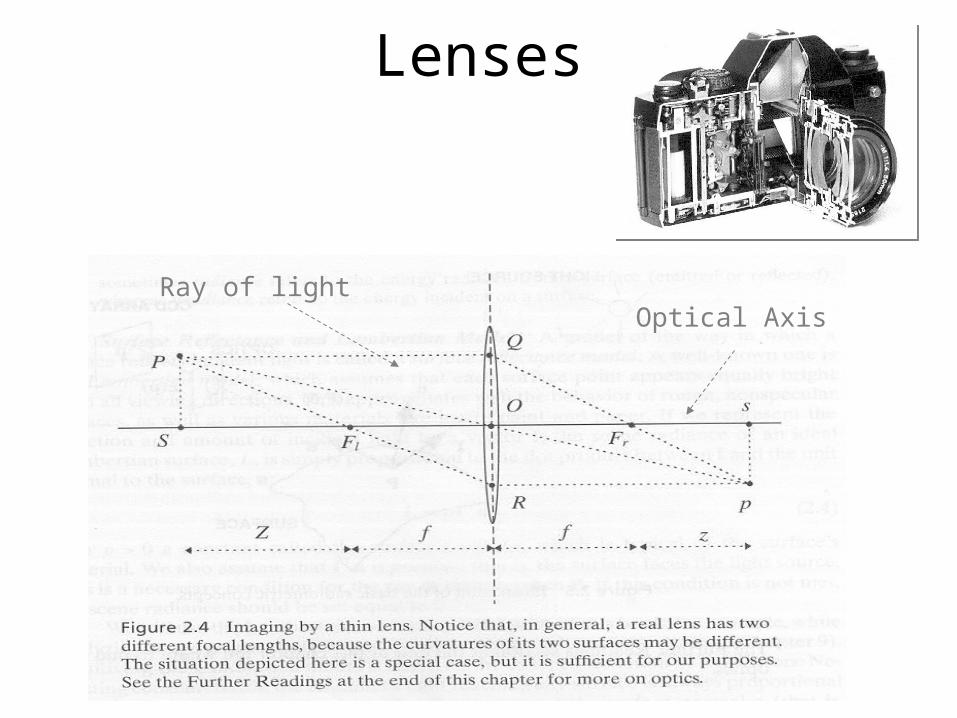
Lenses
Ray of lightOptical Axis
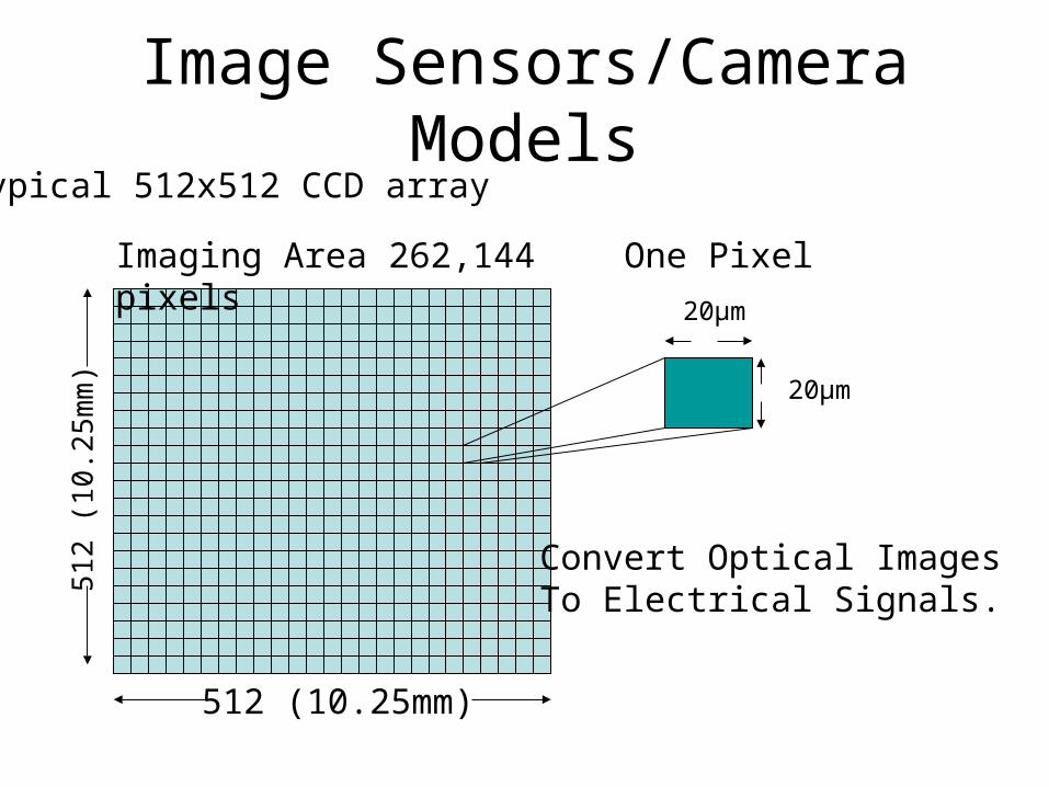
Image Sensors/Camera ModelsTypical 512x512 CCD array
512 (10.25mm)
5 12
( 10 .
2 5m
m)
One Pixel
20μm
20μm
Imaging Area 262,144 pixels
Convert Optical ImagesTo Electrical Signals.
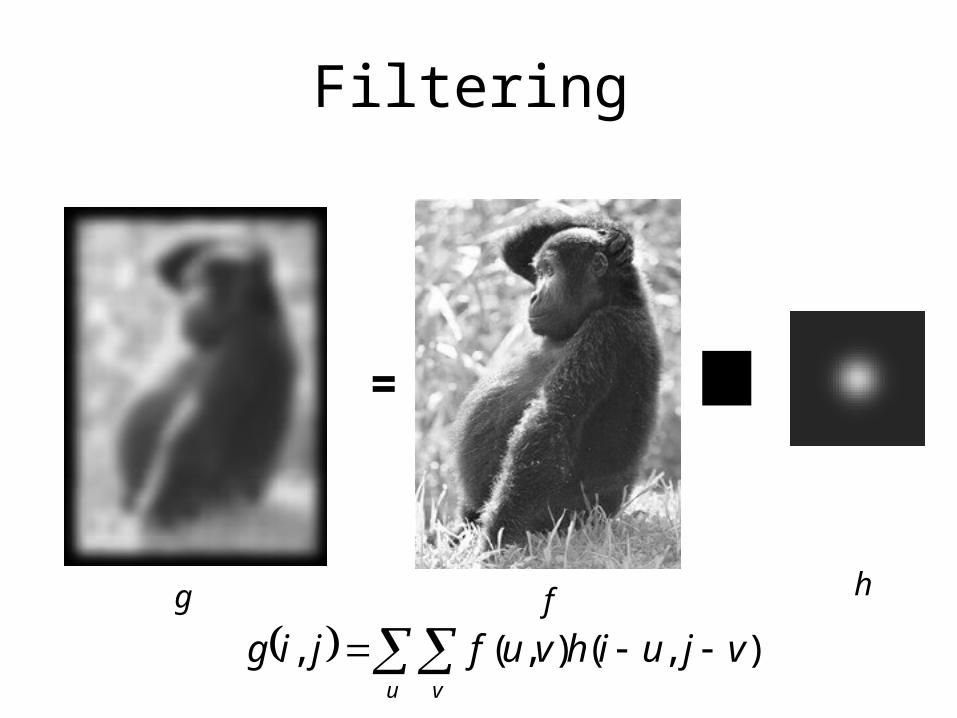
Filtering
=
u v
vjuihvufjig ),(),(,
g hf
Ioannis Stamos – CSc 83020 Spring 2007
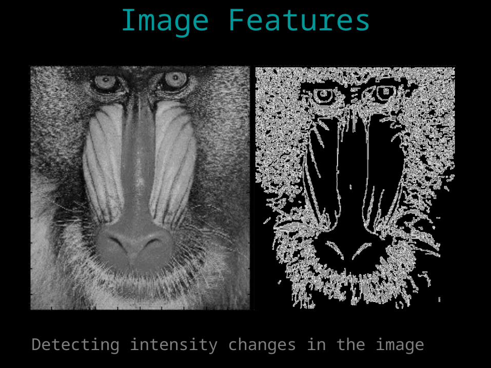
Image Features
Detecting intensity changes in the image
Ioannis Stamos – CSc 83020 Spring 2007
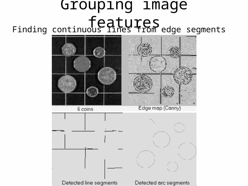
Grouping image featuresFinding continuous lines from edge segments
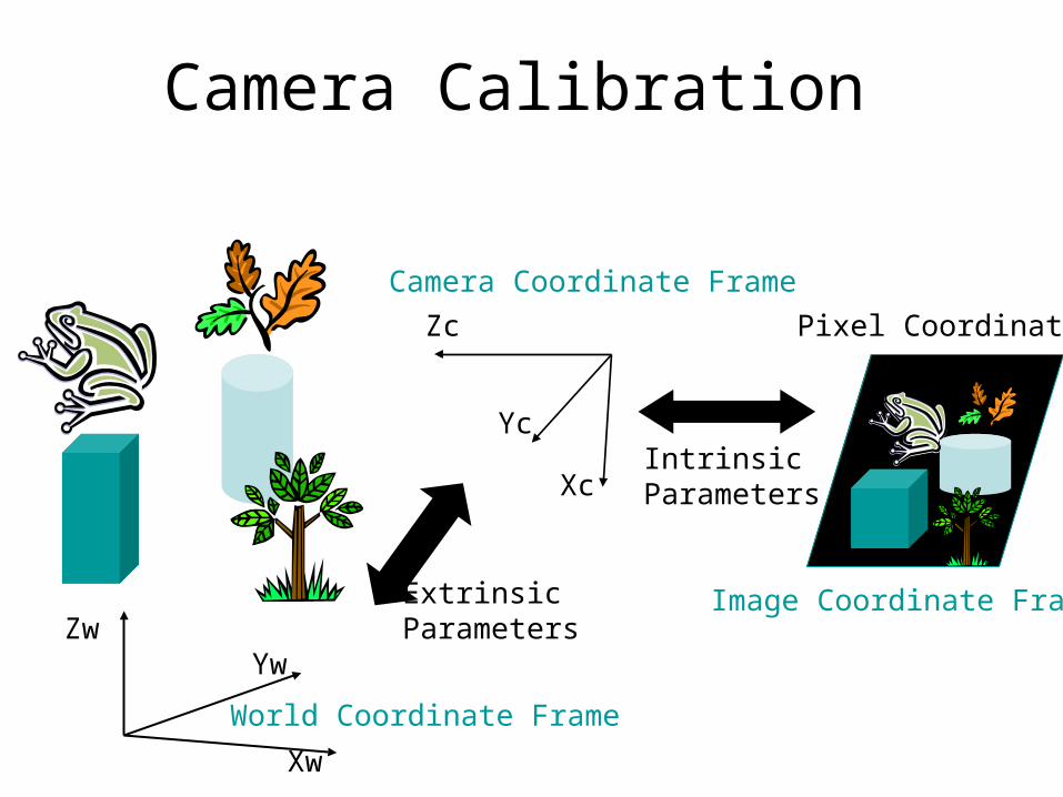
Camera Calibration
Xw
YwZw
World Coordinate Frame
Xc
Yc
Zc
Camera Coordinate Frame
Image Coordinate Frame
Pixel Coordinates
IntrinsicParameters
ExtrinsicParameters
Shape from X
• Shape from X– Stereo– Motion– Shading– Texture foreshortening
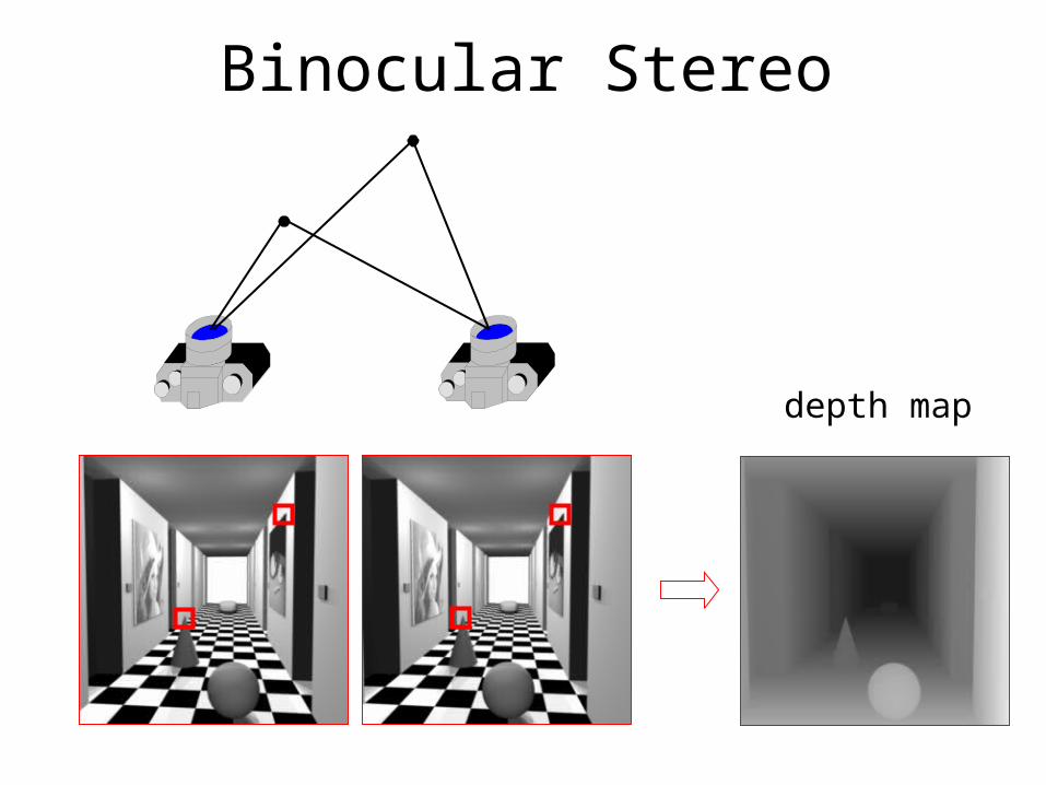
Binocular Stereo
depth map
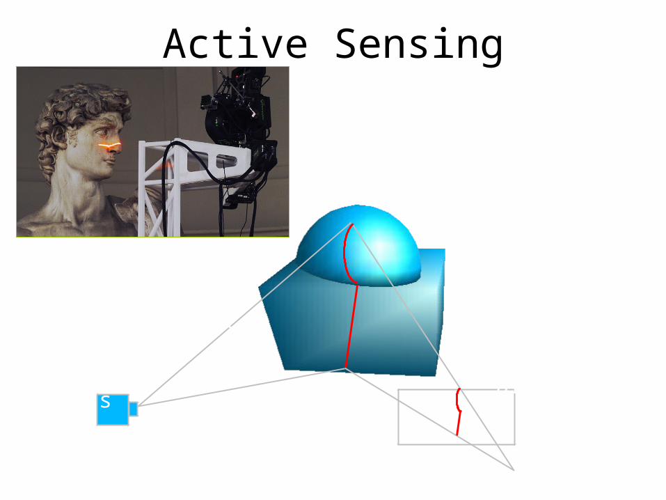
Active Sensing
Lens
Sheet oflight
CCD array
Sources of error: 1) grazing angle, 2) object boundaries.
Ioannis Stamos – CSc 83020 Spring 2007
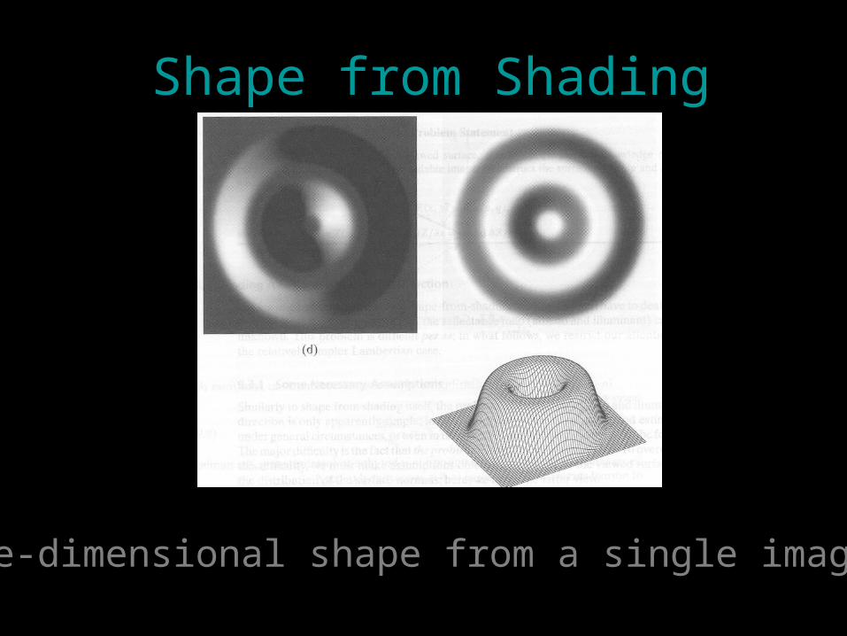
Shape from Shading
Three-dimensional shape from a single image.
Ioannis Stamos – CSc 83020 Spring 2007
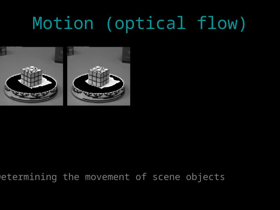
Motion (optical flow)
Determining the movement of scene objects
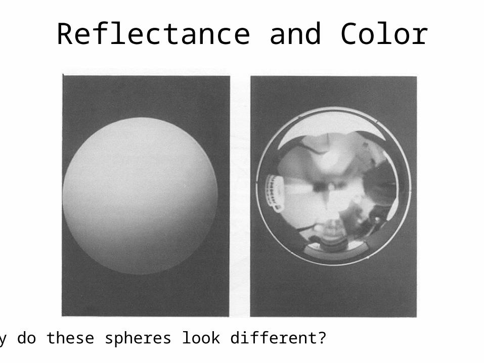
Reflectance and Color
Why do these spheres look different?
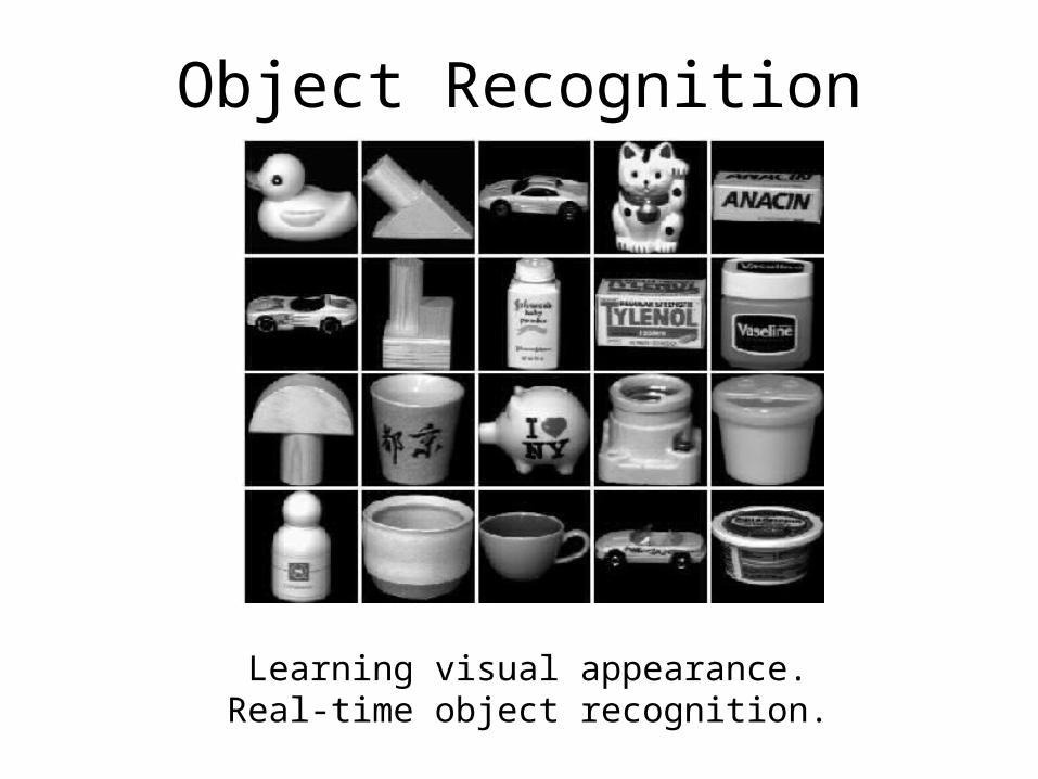
Object Recognition
Learning visual appearance.Real-time object recognition.
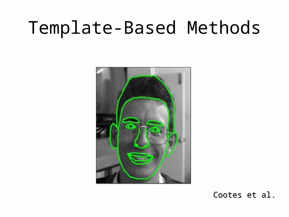
Cootes et al.Cootes et al.
Template-Based Methods

Some Vision Systems…
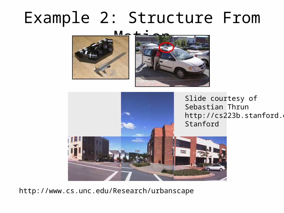
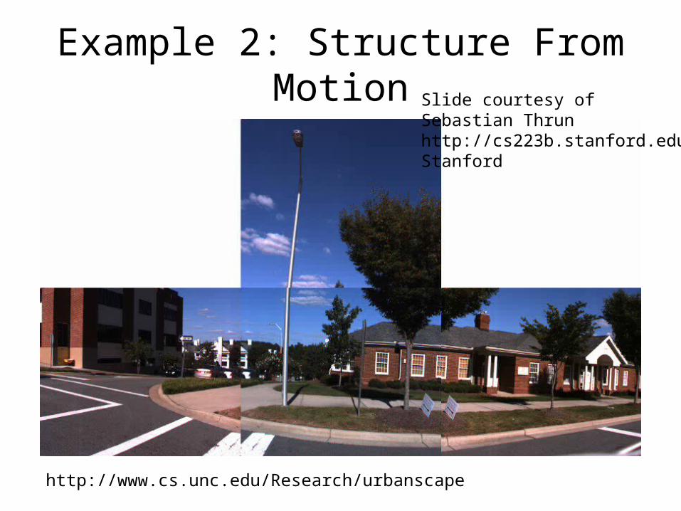
Example 2: Structure From Motion
http://www.cs.unc.edu/Research/urbanscape
Slide courtesy ofSebastian Thrun http://cs223b.stanford.eduStanford
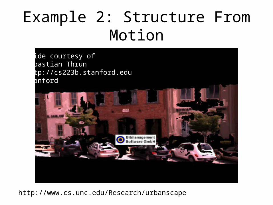
Example 2: Structure From Motion
http://www.cs.unc.edu/Research/urbanscape
Slide courtesy ofSebastian Thrun http://cs223b.stanford.eduStanford
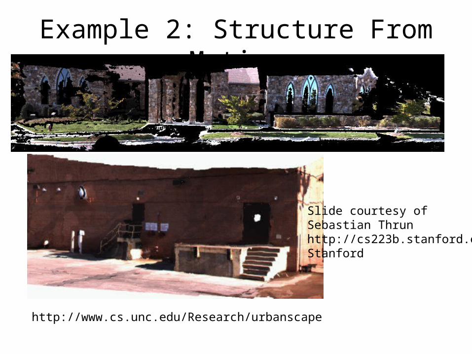
Example 2: Structure From Motion
http://www.cs.unc.edu/Research/urbanscape
Slide courtesy ofSebastian Thrun http://cs223b.stanford.eduStanford
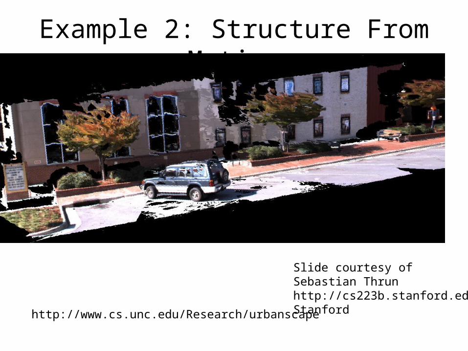
Example 2: Structure From Motion
http://www.cs.unc.edu/Research/urbanscape
Slide courtesy ofSebastian Thrun http://cs223b.stanford.eduStanford
Example 2: Structure From Motion
http://www.cs.unc.edu/Research/urbanscape
Slide courtesy ofSebastian Thrun http://cs223b.stanford.eduStanford
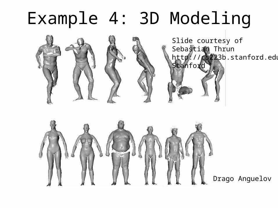
Example 4: 3D Modeling
Drago Anguelov
Slide courtesy ofSebastian Thrun http://cs223b.stanford.eduStanford
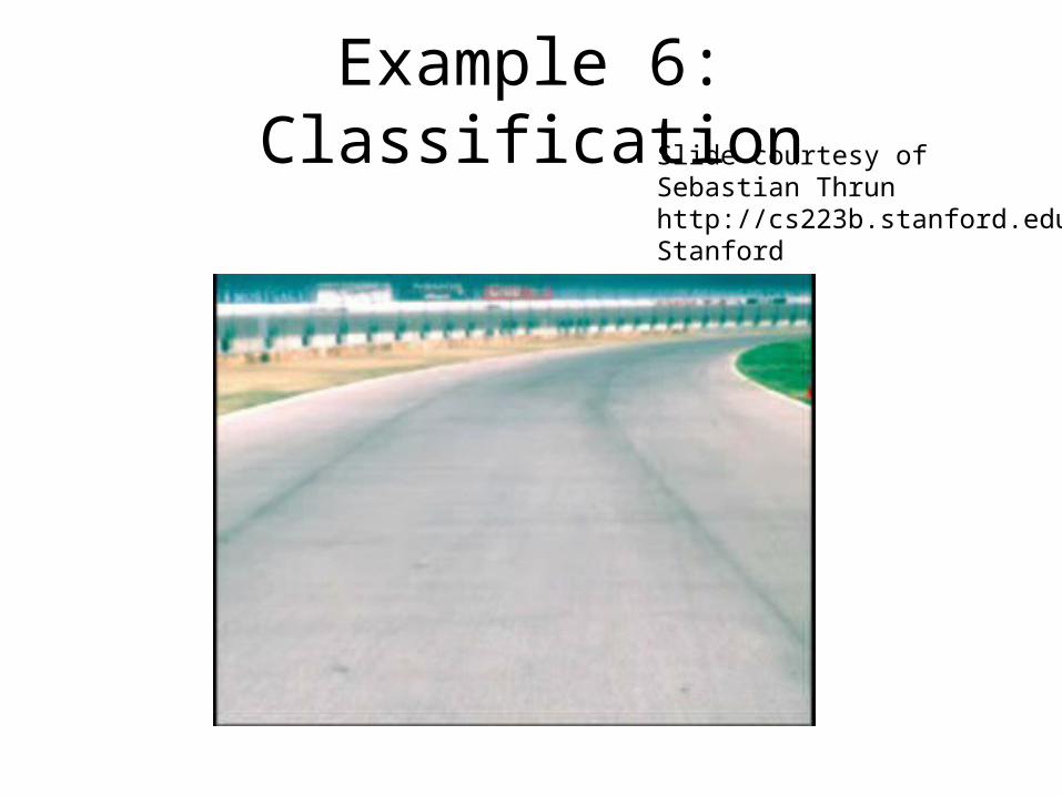
Example 6: ClassificationSlide courtesy ofSebastian Thrun http://cs223b.stanford.eduStanford
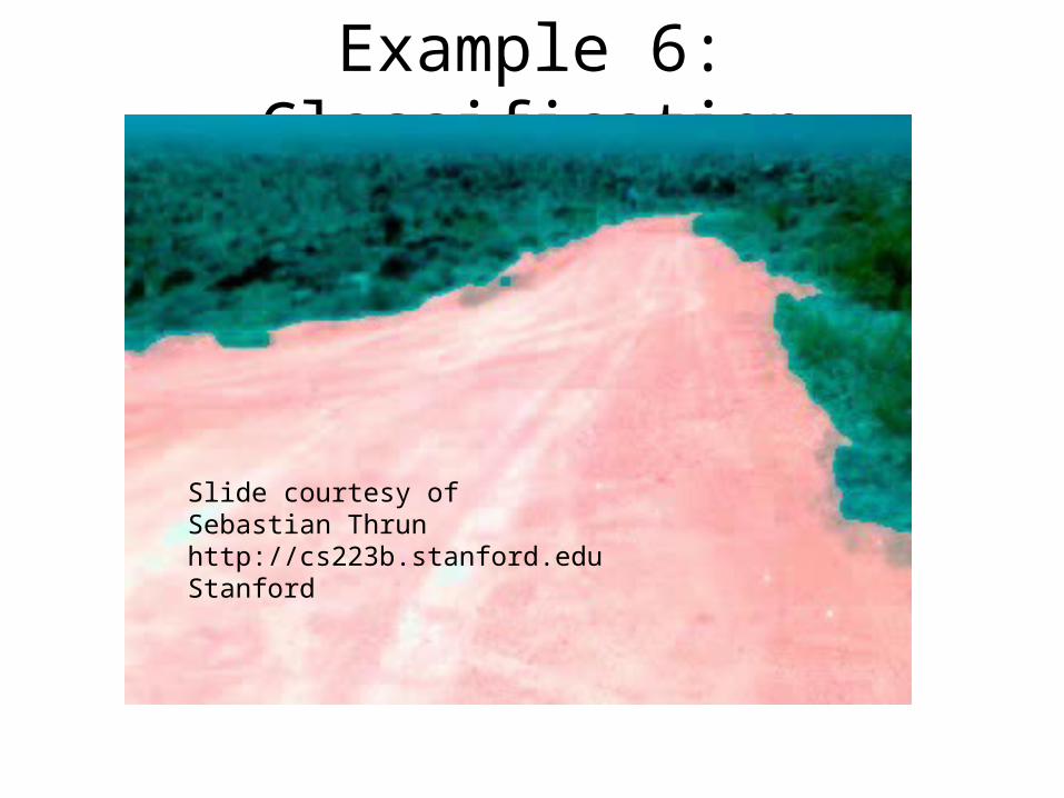
Example 6: Classification
Slide courtesy ofSebastian Thrun http://cs223b.stanford.eduStanford
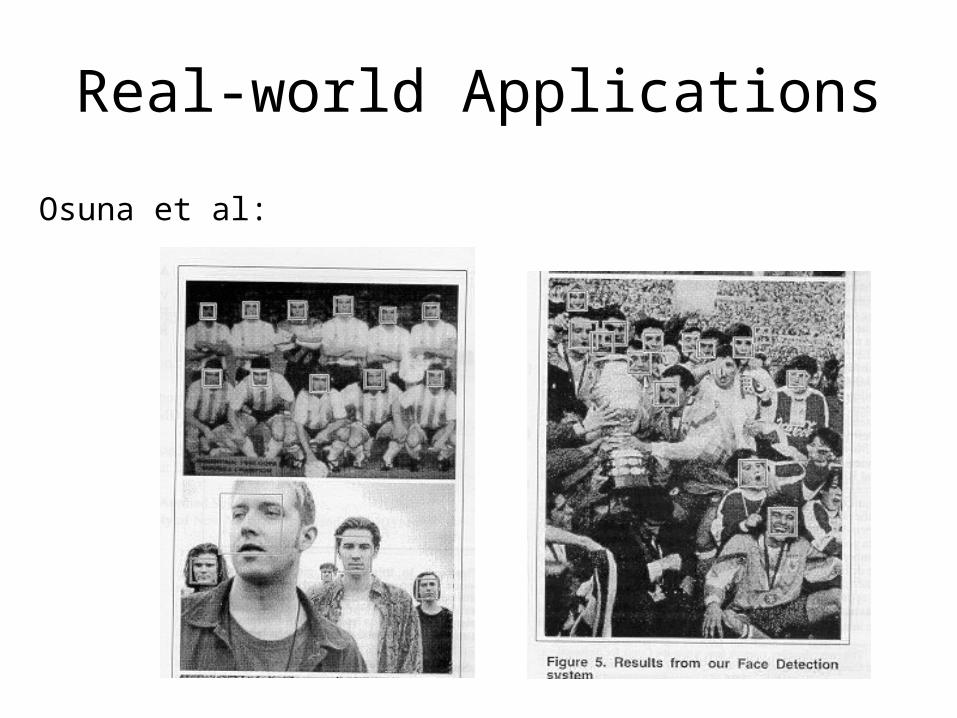
Real-world Applications
Osuna et al:
Ioannis Stamos – CSc 83020 Spring 2007
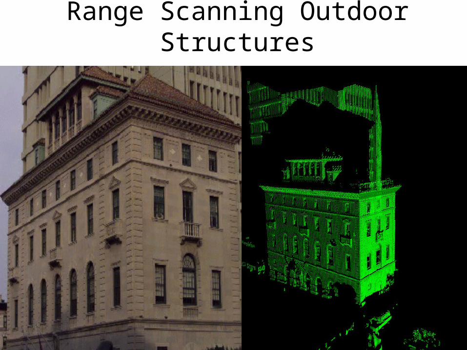
Range Scanning Outdoor Structures
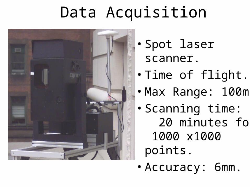
Data Acquisition
• Spot laser scanner.
• Time of flight.
• Max Range: 100m.
• Scanning time: 20 minutes for 1000 x1000 points.
• Accuracy: 6mm.
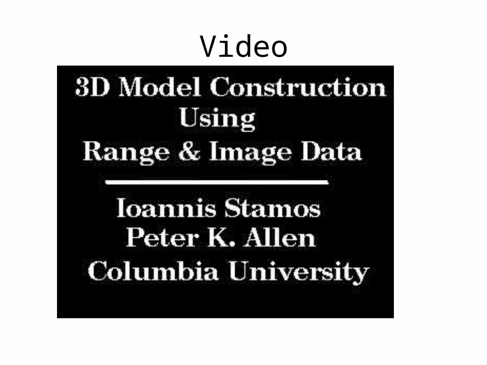
Video
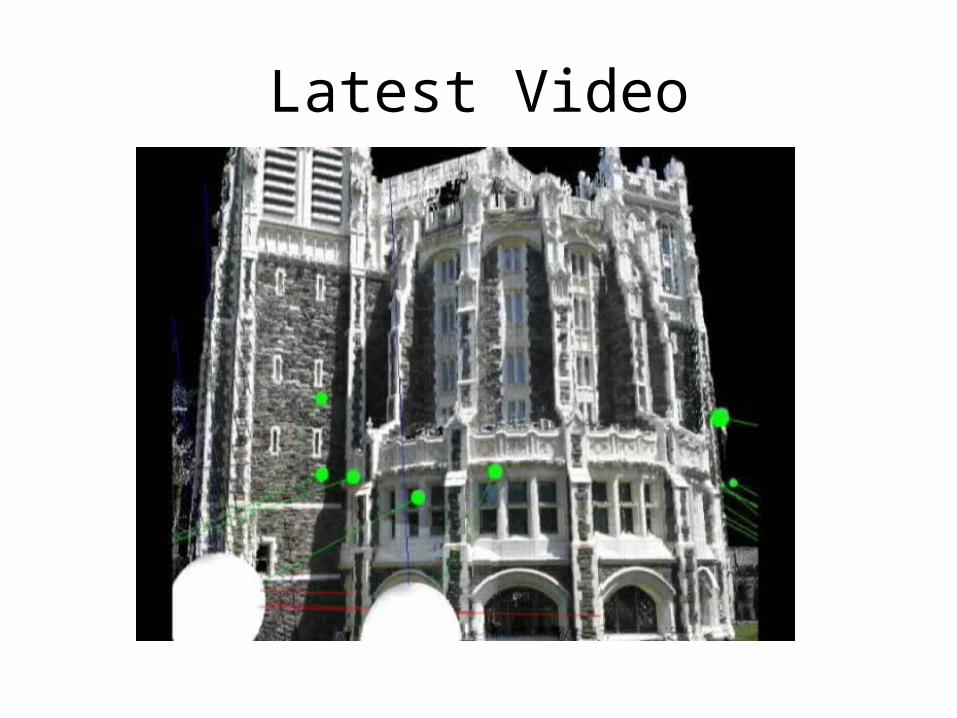
Latest Video
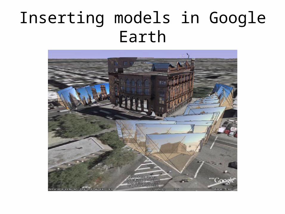
Inserting models in Google Earth
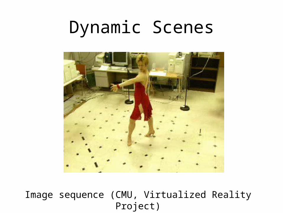
Dynamic Scenes
Image sequence (CMU, Virtualized Reality Project)
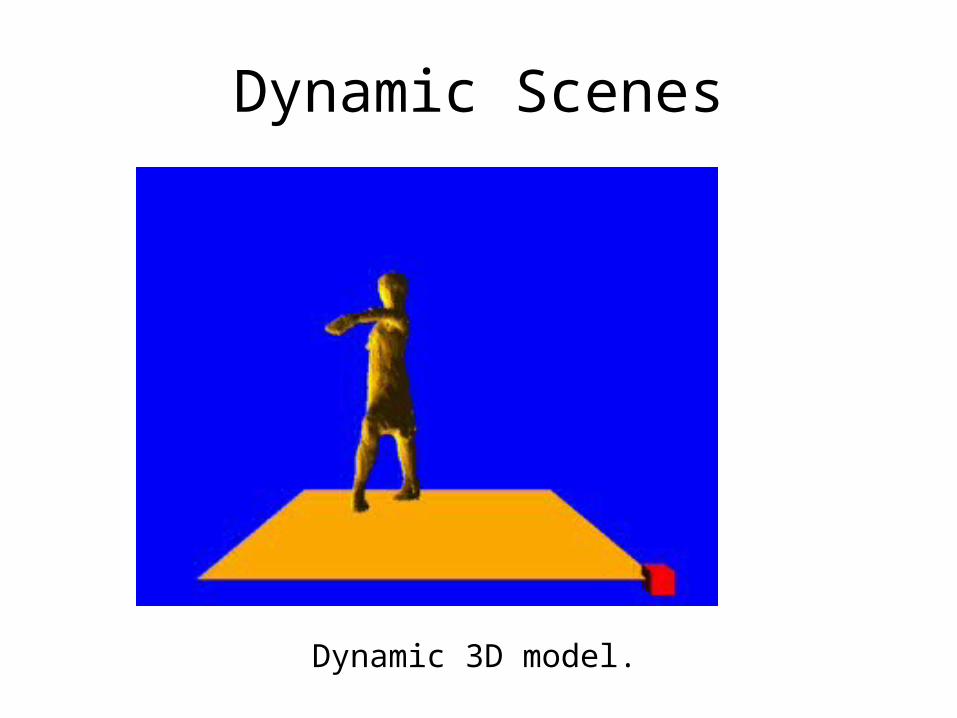
Dynamic Scenes
Dynamic 3D model.
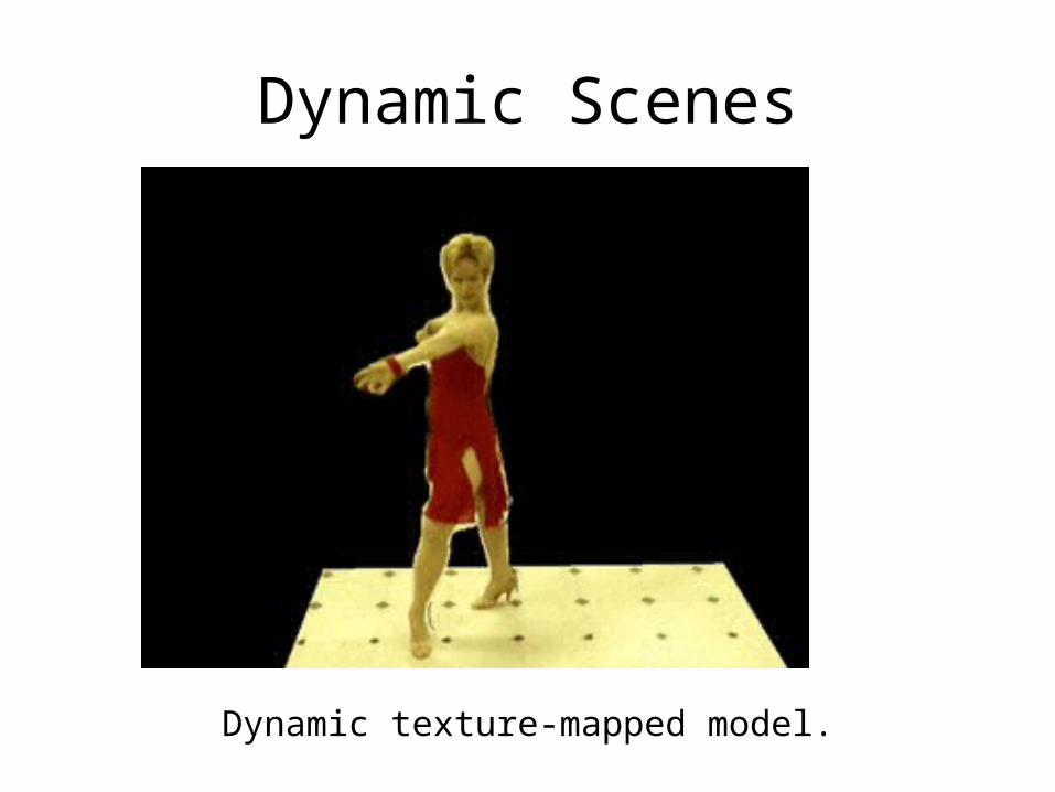
Dynamic Scenes
Dynamic texture-mapped model.

Scanning the DavidMarc Levoy, Stanford
height of gantry: 7.5 meters
weight of gantry: 800 kilograms
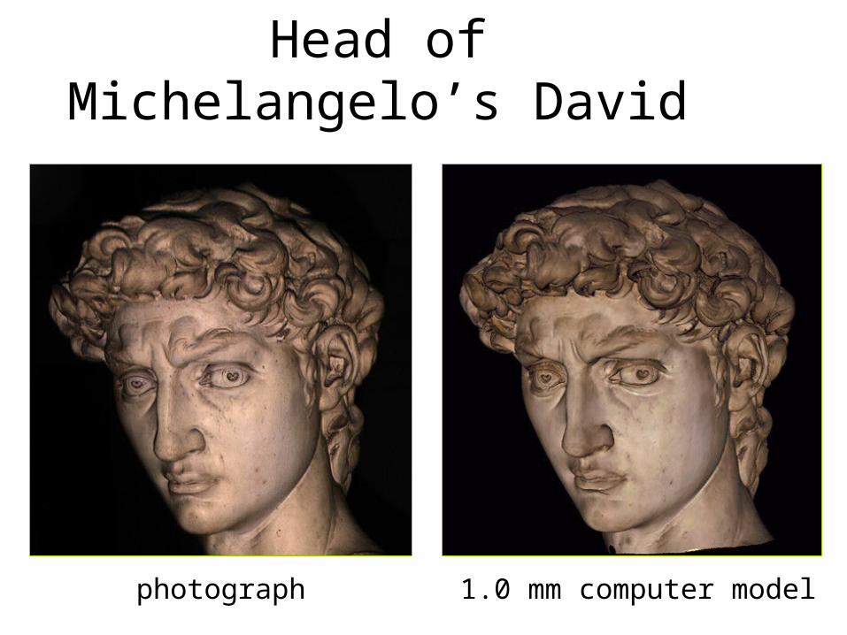
Head of Michelangelo’s David
photograph 1.0 mm computer model

What do you think?