1

3D Digitization Project: 3D Tracking using ActiveAppearance Models

Guillaume Lemaıtre, Mojdeh Rastgoo and Rocio Cabrera LozoyaHeriot-Watt University, Universitat de Girona, Universite de Bourgogne

g.lemaitre58@gmail.com

Abstract—This paper describes a face tracking algorithm usingmodel-based methods and more precisely Active AppearanceModels (AAM). First, an introduction on the background theoryabout model-based methods on machine vision is presented, fol-lowed by a description on statistical shape models and statisticalmodels of appearance, which are necessary to develop AAMs.The implementation description, done in a Matlab programmingenvironment, is presented and its final results.

I. INTRODUCTION

Face detection is a necessary step in many applications,ranging from content-based image retrieval and video coding,to intelligent human-computer interfaces, crowd surveillance,biometric identification, and video conferencing [1] . A widerange of face detection techniques exist, from simple algo-rithms to advanced composite high level approaches for patternrecognition, as the problem has received attention over the lastfifteen years.

For offline processing, the technology has reach a pointwhere the face detection problem is nearly closed [1] ,although accurate detection of features such as corners of eyesor lips is more difficult. However, face detection in real-timeis still an open problem, as the best algorithms are still tocomputationally expensive for real-time processing.

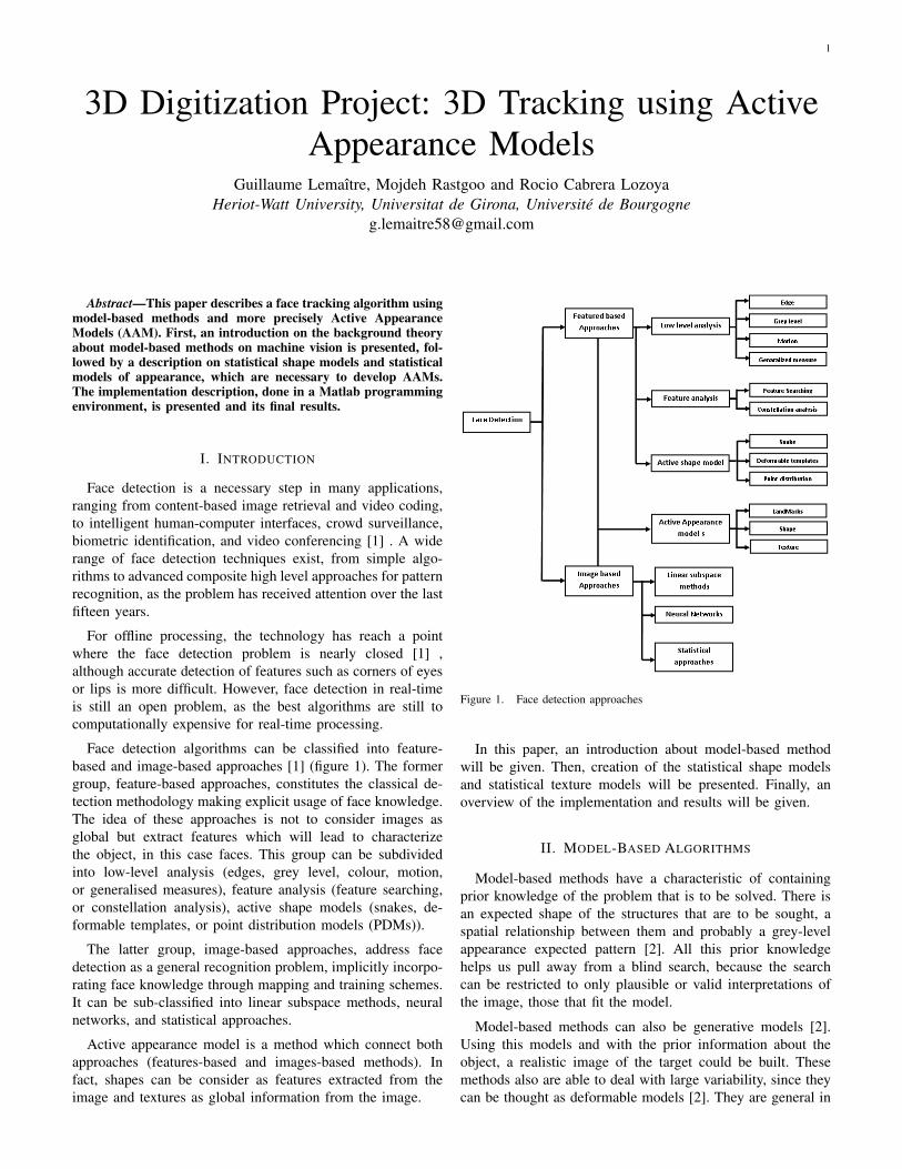
Face detection algorithms can be classified into feature-based and image-based approaches [1] (figure 1). The formergroup, feature-based approaches, constitutes the classical de-tection methodology making explicit usage of face knowledge.The idea of these approaches is not to consider images asglobal but extract features which will lead to characterizethe object, in this case faces. This group can be subdividedinto low-level analysis (edges, grey level, colour, motion,or generalised measures), feature analysis (feature searching,or constellation analysis), active shape models (snakes, de-formable templates, or point distribution models (PDMs)).

The latter group, image-based approaches, address facedetection as a general recognition problem, implicitly incorpo-rating face knowledge through mapping and training schemes.It can be sub-classified into linear subspace methods, neuralnetworks, and statistical approaches.

Active appearance model is a method which connect bothapproaches (features-based and images-based methods). Infact, shapes can be consider as features extracted from theimage and textures as global information from the image.

Figure 1. Face detection approaches

In this paper, an introduction about model-based methodwill be given. Then, creation of the statistical shape modelsand statistical texture models will be presented. Finally, anoverview of the implementation and results will be given.

II. MODEL-BASED ALGORITHMS

Model-based methods have a characteristic of containingprior knowledge of the problem that is to be solved. There isan expected shape of the structures that are to be sought, aspatial relationship between them and probably a grey-levelappearance expected pattern [2]. All this prior knowledgehelps us pull away from a blind search, because the searchcan be restricted to only plausible or valid interpretations ofthe image, those that fit the model.

Model-based methods can also be generative models [2].Using this models and with the prior information about theobject, a realistic image of the target could be built. Thesemethods also are able to deal with large variability, since theycan be thought as deformable models [2]. They are general in

2

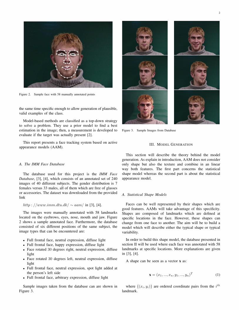
Figure 2. Sample face with 58 manually annotated points

the same time specific enough to allow generation of plausible,valid examples of the class.

Model-based methods are classified as a top-down strategyto solve a problem. They use a prior model to find a bestestimation in the image; then, a measurement is developed toevaluate if the target was actually present [2].

This report presents a face tracking system based on activeappearance models (AAM).

A. The IMM Face Database

The database used for this project is the IMM FaceDatabase, [3], [4], which consists of an annotated set of 240images of 40 different subjects. The gender distribution is 7females versus 33 males, all of them which are free of glassesor accessories. The dataset was downloaded from the providedlink

http : //www.imm.dtu.dk/ ∼ aam/ in [3], [4].

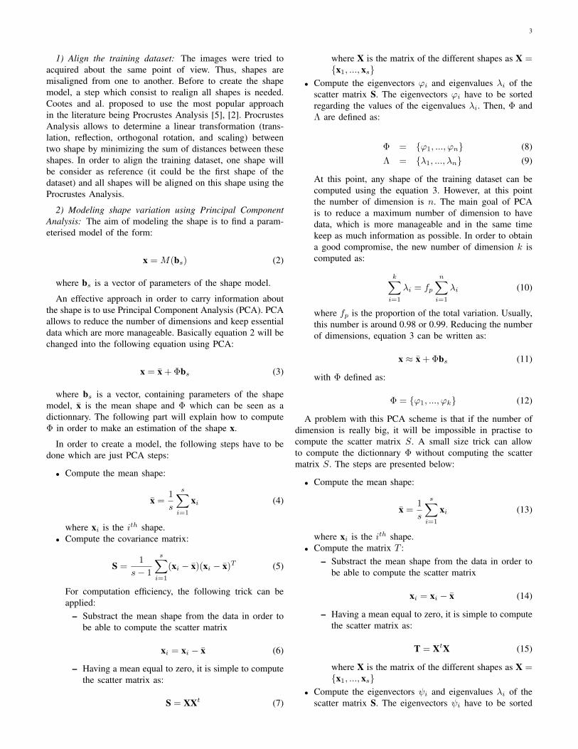
The images were manually annotated with 58 landmarkslocated on the eyebrows, eyes, nose, mouth and jaw. Figure2 shows a sample annotated face. Furthermore, the databaseconsisted of six different positions of the same subject, theimage types that can be encountered are:

• Full frontal face, neutral expression, diffuse light• Full frontal face, happy expression, diffuse light• Face rotated 30 degrees right, neutral expression, diffuse

light• Face rotated 30 degrees left, neutral expression, diffuse

light• Full frontal face, neutral expression, spot light added at

the person’s left side• Full frontal face, arbitrary expression, diffuse light

Sample images taken from the database can are shown inFigure 3.

Figure 3. Sample Images from Database

III. MODEL GENERATION

This section will describe the theory behind the modelgeneration. As explain in introduction, AAM does not consideronly shape but also the texture and combine in an linearway both features. The first part concerns the statisticalshape model whereas the second part is about the statisticalappearance model.

A. Statistical Shape Models

Faces can be well represented by their shapes which aregood features. AAMs will take advantage of this specificity.Shapes are composed of landmarks which are defined atspecific locations in the face. However, these shapes canchange from one face to another. The aim will be to build amodel which will describe either the typical shape or typicalvariability.

In order to build this shape model, the database presented insection II will be used where each face was annotated with 58landmarks at specific locations. More explanations are givenin [3], [4].

A shape can be seen as a vector x as:

x = (x1, ..., xn, y1, ..., yn)T (1)

where {(xi, yi)} are ordered coordinate pairs from the ith

landmark.

3

1) Align the training dataset: The images were tried toacquired about the same point of view. Thus, shapes aremisaligned from one to another. Before to create the shapemodel, a step which consist to realign all shapes is needed.Cootes and al. proposed to use the most popular approachin the literature being Procrustes Analysis [5], [2]. ProcrustesAnalysis allows to determine a linear transformation (trans-lation, reflection, orthogonal rotation, and scaling) betweentwo shape by minimizing the sum of distances between theseshapes. In order to align the training dataset, one shape willbe consider as reference (it could be the first shape of thedataset) and all shapes will be aligned on this shape using theProcrustes Analysis.

2) Modeling shape variation using Principal ComponentAnalysis: The aim of modeling the shape is to find a param-eterised model of the form:

x = M(bs) (2)

where bs is a vector of parameters of the shape model.

An effective approach in order to carry information aboutthe shape is to use Principal Component Analysis (PCA). PCAallows to reduce the number of dimensions and keep essentialdata which are more manageable. Basically equation 2 will bechanged into the following equation using PCA:

x = x + Φbs (3)

where bs is a vector, containing parameters of the shapemodel, x is the mean shape and Φ which can be seen as adictionnary. The following part will explain how to computeΦ in order to make an estimation of the shape x.

In order to create a model, the following steps have to bedone which are just PCA steps:

• Compute the mean shape:

x =1

s

s∑i=1

xi (4)

where xi is the ith shape.• Compute the covariance matrix:

S =1

s− 1

s∑i=1

(xi − x)(xi − x)T (5)

For computation efficiency, the following trick can beapplied:

– Substract the mean shape from the data in order tobe able to compute the scatter matrix

xi = xi − x (6)

– Having a mean equal to zero, it is simple to computethe scatter matrix as:

S = XXt (7)

where X is the matrix of the different shapes as X ={x1, ..., xs}

• Compute the eigenvectors ϕi and eigenvalues λi of thescatter matrix S. The eigenvectors ϕi have to be sortedregarding the values of the eigenvalues λi. Then, Φ andΛ are defined as:

Φ = {ϕ1, ..., ϕn} (8)Λ = {λ1, ..., λn} (9)

At this point, any shape of the training dataset can becomputed using the equation 3. However, at this pointthe number of dimension is n. The main goal of PCAis to reduce a maximum number of dimension to havedata, which is more manageable and in the same timekeep as much information as possible. In order to obtaina good compromise, the new number of dimension k iscomputed as:

k∑i=1

λi = fp

n∑i=1

λi (10)

where fp is the proportion of the total variation. Usually,this number is around 0.98 or 0.99. Reducing the numberof dimensions, equation 3 can be written as:

x ≈ x + Φbs (11)

with Φ defined as:

Φ = {ϕ1, ..., ϕk} (12)

A problem with this PCA scheme is that if the number ofdimension is really big, it will be impossible in practise tocompute the scatter matrix S. A small size trick can allowto compute the dictionnary Φ without computing the scattermatrix S. The steps are presented below:

• Compute the mean shape:

x =1

s

s∑i=1

xi (13)

where xi is the ith shape.• Compute the matrix T :

– Substract the mean shape from the data in order tobe able to compute the scatter matrix

xi = xi − x (14)

– Having a mean equal to zero, it is simple to computethe scatter matrix as:

T = XtX (15)

where X is the matrix of the different shapes as X ={x1, ..., xs}

• Compute the eigenvectors ψi and eigenvalues λi of thescatter matrix S. The eigenvectors ψi have to be sorted

4

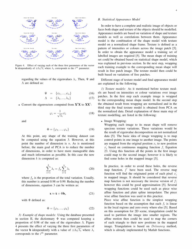
Figure 4. Effect of varying each of the three first parameters of the vectorb idenpendently of ±3

√λi where λi corresponds to the ith parameter.

regarding the values of the eigenvalues λi. Then, Ψ andΛ are defined as:

Ψ = {ψ1, ..., ψn} (16)Λ = {λ1, ..., λn} (17)

• Convert the eigenvectors computed from XtX to XXt:

ϕi =1√λiψi (18)

and

Φ = {ϕ1, ..., ϕn} (19)

At this point, any shape of the training dataset canbe computed using the equation 3. However, at thispoint the number of dimension is n. As is mentionedbefore, the main goal of PCA is to reduce the numberof dimensions, in order to have more manageable dataand much information as possible. In this case the newdimension k is computed as:

k∑i=1

λi = fp

n∑i=1

λi (20)

where fp is the proportion of the total variation. Usually,this number is around 0.98 or 0.99. Reducing the numberof dimensions, equation 3 can be written as:

x ≈ x + Φbs (21)

with Φ defined as:

Φ = {ϕ1, ..., ϕk} (22)

3) Example of shape models: Using the database presentedin section II, the dictionnary Φ was computed keeping aproportion of 0.98 of the sum of the eigenvalues Λ. Figure4 presents the effect of varying the three first parameters ofthe vector b idenpendently with a value of ±3

√λi where λi

corresponds to the ith parameter.

B. Statistical Appearance Model

In order to have a complete and realistic image of objects orfaces both shape and texture of the objects should be modelled.Appearance models are based on variation of shape and texturemodels as well as correlations between them. Appearancemodel is the combination of the shape model with texturemodel on a normalized shape frame. Texture is defined as apattern of intensities or colours across the image patch [5].In order to obtain the appearance model a training set oflabelled images are required [5]. The mean shape of trainingset could be obtained based on statistical shape model, whichwas explained in previous section. In the next step, wrappingeach training example to the corresponding mean shape willresult in free patch image. The texture model then could bebuilt based on variations of free patches.

Different stage of texture model and final appearance modelare explained in the following.

1) Texture models: As it mentioned before texture mod-els are based on intensities or colour variations over imagepatches. In the first step each example image is wrappedto the corresponding mean shape model. In the second stepthe obtained result from wrapping are normalized and in thethird step the final texture model is obtained from PCA onthe normalized data. Detail explanation of three main step oftexture modelling, are listed in the following:

• Image Wrapping:Wrapping each image to its mean shape will removespecious texture variations. These variations would bethe result of eigenvalue decomposition on not normalizeddata [5]. The basic idea of image wrapping is to mapcontrol points in one image to another image. The pointsare mapped from the original position xi to new positionx

′

i based on continuous mapping function f , Equation23. Using this function all the points in the first imagecould map to the second image; however it is likely tofind some holes in the mapped image [5].

In practice, in order to avoid these holes, the reversemap function, f

′have been used. The reverse map

function will find the originated point of each pixel x′

i

in mapped image. It should be considered that reversemap function is not necessary the inverse version of f ;however this could be good approximation [5]. Severalwrapping functions could be used such as piece wiseaffine function and plate spline interpolator. The piecewise affine function was used in this practice.Piece wise affine function is the simplest wrappingfunction based on the assumption that each fi is linearin the local regions and zero every where else [5]. Basedon this assumption for 2D scene, triangulation could beused to partition the image into smaller regions. Theaffine motion then could be used to map the cornersof each triangle to their new positions in the mappedimage. Triangulation is based on Delauney method,which is already implemented by Matlab functions.

5

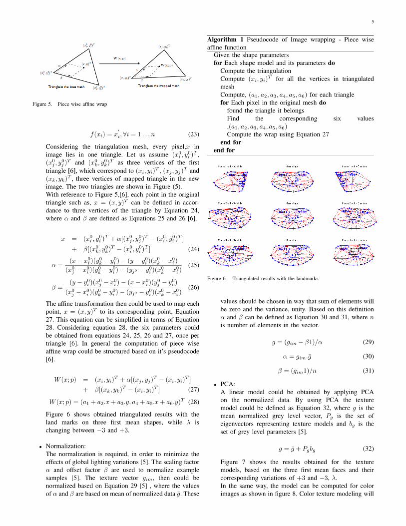
Figure 5. Piece wise affine wrap

f(xi) = x′

i,∀i = 1 . . . n (23)

Considering the triangulation mesh, every pixel,x inimage lies in one triangle. Let us assume (x0i , y

0i )T ,

(x0j , y0j )T and (x0k, y

0k)T as three vertices of the first

triangle [6], which correspond to (xi, yi)T , (xj , yj)

T and(xk, yk)T , three vertices of mapped triangle in the newimage. The two triangles are shown in Figure (5).With reference to Figure 5,[6], each point in the originaltriangle such as, x = (x, y)T can be defined in accor-dance to three vertices of the triangle by Equation 24,where α and β are defined as Equations 25 and 26 [6].

x = (x0i , y0i )T + α[(x0j , y

0j )T − (x0i , y

0i )T ]

+ β[(x0k, y0k)T − (x0i , y

0i )T ] (24)

α =(x− x0i )(y0k − y0i )− (y − y0i )(x0k − x0i )

(x0j − x0i )(y0k − y0i )− (yj0 − y0i )(x0k − x0i )(25)

β =(y − y0i )(x0j − x0i )− (x− x0i )(y0j − y0i )

(x0j − x0i )(y0k − y0i )− (yj0 − y0i )(x0k − x0i )(26)

The affine transformation then could be used to map eachpoint, x = (x, y)T to its corresponding point, Equation27. This equation can be simplified in terms of Equation28. Considering equation 28, the six parameters couldbe obtained from equations 24, 25, 26 and 27, once pertriangle [6]. In general the computation of piece wiseaffine wrap could be structured based on it’s pseudocode[6].

W (x; p) = (xi, yi)T + α[(xj , yj)

T − (xi, yi)T ]

+ β[(xk, yk)T − (xi, yi)T ] (27)

W (x; p) = (a1 + a2.x+ a3.y, a4 + a5.x+ a6.y)T (28)

Figure 6 shows obtained triangulated results with theland marks on three first mean shapes, while λ ischanging between −3 and +3.

• Normalization:The normalization is required, in order to minimize theeffects of global lighting variations [5]. The scaling factorα and offset factor β are used to normalize examplesamples [5]. The texture vector gim, then could benormalized based on Equation 29 [5] , where the valuesof α and β are based on mean of normalized data g. These

Algorithm 1 Pseudocode of Image wrapping - Piece wiseaffine function

Given the shape parametersfor Each shape model and its parameters do

Compute the triangulationCompute (xi, yi)

T for all the vertices in triangulatedmeshCompute, (a1, a2, a3, a4, a5, a6) for each trianglefor Each pixel in the original mesh do

found the triangle it belongsFind the corresponding six values,(a1, a2, a3, a4, a5, a6)Compute the wrap using Equation 27

end forend for

Figure 6. Triangulated results with the landmarks

values should be chosen in way that sum of elements willbe zero and the variance, unity. Based on this definitionα and β can be defined as Equation 30 and 31, where nis number of elements in the vector.

g = (gim − β1)/α (29)

α = gim.g (30)

β = (gim1)/n (31)

• PCA:A linear model could be obtained by applying PCAon the normalized data. By using PCA the texturemodel could be defined as Equation 32, where g is themean normalized grey level vector, Pg is the set ofeigenvectors representing texture models and bg is theset of grey level parameters [5].

g = g + Pgbg (32)

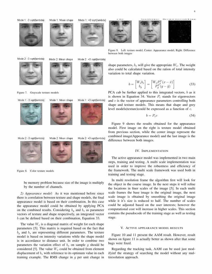
Figure 7 shows the results obtained for the texturemodels, based on the three first mean faces and theircorresponding variations of +3 and −3, λ.In the same way, the model can be computed for colorimages as shown in figure 8. Color texture modeling will

6

Figure 7. Grayscale texture models

Figure 8. Color texture models

be memory problem because size of the image is multiplyby the number of channels.

2) Appearance model: As it was mentioned before sincethere is correlation between texture and shape models, the finalappearance model is based on their combination. In this casethe appearance model could be obtained by applying PCAon the combined results. Considering bg and bs as parametervectors of texture and shape respectively, an integrated vectorb can be defined based on their combination, Equation 33.

The value Ws is a diagonal matrix of weight for each shapeparameters [5]. This matrix is required based on the fact thatbg and bs are representing different parameters. The texturemodel is based on intensity variations while the shape modelis in accordance to distance unit. In order to combine twoparameters the variation effect of bs on sample g should beconsidered [5]. The value Ws could be obtained from elementdisplacement of bs with reference to its optimum value in eachtraining example. The RMS change in g per unit change in

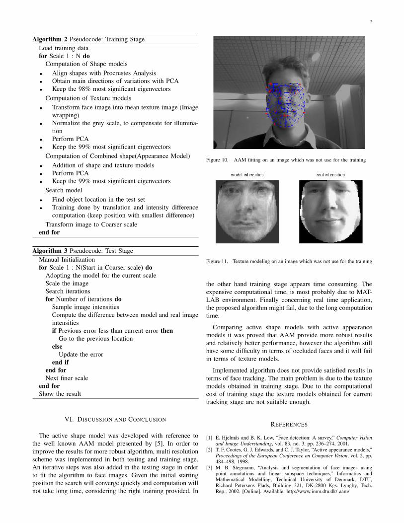
Figure 9. Left: texture model, Center: Appearance model, Right: Differencebetween both images

shape parameters, bs will give the appropriate Ws. The weightalso could be calculated based on the ration of total intensityvariation to total shape variation.

b =

[Wsbsbg

]=

[WsP

Ts (x− x)

PTg (g − g)

](33)

PCA cab be further applied to this integrated vectors, b as itis shown in Equation 34. Vector Pc stands for eigenvectorsand c is the vector of appearance parameters controlling bothshape and texture models. This means that shape and greylevel models(texture)could be expressed as a function of c.

b = Pcc (34)

Figure 9 shows the results obtained for the appearancemodel. First image on the right is texture model obtainedfrom previous section, while the center image represent thecombined image(Appearance model) and the last image is thedifference between both images.

IV. IMPLEMENTATION

The active appearance model was implemented in two mainsteps, training and testing. A multi scale implementation wasused in order to improve the robustness and efficiency ofthe framework. The multi scale framework was used both intraining and testing stage.

In multi resolution frame the algorithm first will look forthe object in the coarse image. In the next steps it will refinethe locations in finer scales of the image [5]. In each multiscale frames the base image is the original image, the nextscale image is obtained by smoothing the original imagewhile it it’s size is reduced to half. The number of scalescould be adjusted based on the user interests; however thecomputational cost will increase in higher scales. This sectioncontains the pseudocode of the training stage as well as testingstage.

V. ACTIVE APPEARANCE MODEL RESULTS

Figure 10 and 11 present the AAM result. However, resultshown on figure 11 is actually better as shown after that somebugs were fixed.

Regarding the tracking task, AAM can be used just mod-ifyinf the strategy of searching the model without any mul-tiresolution approach.

7

Algorithm 2 Pseudocode: Training StageLoad training datafor Scale 1 : N do

Computation of Shape models• Align shapes with Procrustes Analysis• Obtain main directions of variations with PCA• Keep the 98% most significant eigenvectors

Computation of Texture models• Transform face image into mean texture image (Image

wrapping)• Normalize the grey scale, to compensate for illumina-

tion• Perform PCA• Keep the 99% most significant eigenvectors

Computation of Combined shape(Appearance Model)• Addition of shape and texture models• Perform PCA• Keep the 99% most significant eigenvectors

Search model• Find object location in the test set• Training done by translation and intensity difference

computation (keep position with smallest difference)Transform image to Coarser scale

end for

Algorithm 3 Pseudocode: Test StageManual Initializationfor Scale 1 : N(Start in Coarser scale) do

Adopting the model for the current scaleScale the imageSearch iterationsfor Number of iterations do

Sample image intensitiesCompute the difference between model and real imageintensitiesif Previous error less than current error then

Go to the previous locationelse

Update the errorend if

end forNext finer scale

end forShow the result

VI. DISCUSSION AND CONCLUSION

The active shape model was developed with reference tothe well known AAM model presented by [5]. In order toimprove the results for more robust algorithm, multi resolutionscheme was implemented in both testing and training stage.An iterative steps was also added in the testing stage in orderto fit the algorithm to face images. Given the initial startingposition the search will converge quickly and computation willnot take long time, considering the right training provided. In

Figure 10. AAM fitting on an image which was not use for the training

Figure 11. Texture modeling on an image which was not use for the training

the other hand training stage appears time consuming. Theexpensive computational time, is most probably due to MAT-LAB environment. Finally concerning real time application,the proposed algorithm might fail, due to the long computationtime.

Comparing active shape models with active appearancemodels it was proved that AAM provide more robust resultsand relatively better performance, however the algorithm stillhave some difficulty in terms of occluded faces and it will failin terms of texture models.

Implemented algorithm does not provide satisfied results interms of face tracking. The main problem is due to the texturemodels obtained in training stage. Due to the computationalcost of training stage the texture models obtained for currenttracking stage are not suitable enough.

REFERENCES

[1] E. Hjelmas and B. K. Low, “Face detection: A survey,” Computer Visionand Image Understanding, vol. 83, no. 3, pp. 236–274, 2001.

[2] T. F. Cootes, G. J. Edwards, and C. J. Taylor, “Active appearance models,”Proceedings of the European Conference on Computer Vision, vol. 2, pp.484–498, 1998.

[3] M. B. Stegmann, “Analysis and segmentation of face images usingpoint annotations and linear subspace techniques,” Informatics andMathematical Modelling, Technical University of Denmark, DTU,Richard Petersens Plads, Building 321, DK-2800 Kgs. Lyngby, Tech.Rep., 2002. [Online]. Available: http://www.imm.dtu.dk/ aam/

8

[4] M. B. Stegmann, B. K. Ersbøll, and R. Larsen, “FAME – a flexibleappearance modelling environment,” IEEE Trans. on Medical Imaging,vol. 22, no. 10, pp. 1319–1331, 2003.

[5] T. Cootes, C. Taylor, and M. M. Pt, “Statistical models of appearance forcomputer vision,” 2000.

[6] I. Matthews and S. Baker, “Active appearance models revisited,” Inter-national Journal of Computer Vision, vol. 60, pp. 135–164, 2003.