3d facial landmark detection & face...

CGL Technical Report, No. TP-2010-01, January 2010

3D Facial Landmark Detection & Face RegistrationA 3D Facial Landmark Model & 3D Local Shape Descriptors Approach

Panagiotis Perakis1,2, Georgios Passalis1,2, Theoharis Theoharis1,2 and Ioannis A. Kakadiaris2

1 Computer Graphics LaboratoryDepartment of Informatics and TelecommunicationsUniversity of Athens, Ilisia 15784, GREECE2 Computational Biomedicine LabDepartment of Computer ScienceUniversity of Houston, Texas 77204, USA

Abstract In this Technical Report a novel method for 3D landmark detec-tion and pose estimation suitable for both frontal and side 3Dfacial scans is presented. It utilizes 3D information by using 3Dlocal shape descriptors to extract candidate interest points thatare subsequently identified and labeled as anatomical landmarks.The shape descriptors include the shape index, a continuous mapof principal curvature values of 3D objects, the extrusion map, ameasure of the extruded areas of a 3D object and the spin images,local descriptors of the object’s 3D point distribution. However,feature detection methods which use general purpose shape de-scriptors cannot identify and label the detected candidate land-marks. Therefore, the topological properties of the human faceneed to be taken into consideration. To this end, we use a FacialLandmark Model (FLM) of facial anatomical landmarks. Candi-date landmarks, irrespectively of the way they are generated, canbe identified and labeled by matching them with the correspond-ing FLM. The proposed method is evaluated using an extensive3D facial database, and achieves high accuracy even in challengingscenarios.

Keywords Shape Models, Shape Index, Extruded Points, Spin Images, 3DFeature Extraction, Landmark Detection, Pose Estimation.

Version 1.0 Contact info: P. Perakis ([email protected].)

Computer Graphics LaboratoryDepartment of Informatics and TelecommunicationsUniversity of Athens15784 IlisiaGREECEhttp://graphics.di.uoa.gr

3D Facial Landmark Detection & Face Registration

Contents

1 Introduction 1

2 Related Work 2

3 3D Facial Landmark Models 53.1 The Landmark Mean Shape . . . . . . . . . . . . . . . . . . . . . . . 63.2 Shape Alignment Transformations . . . . . . . . . . . . . . . . . . . 83.3 Landmark Shape Variations . . . . . . . . . . . . . . . . . . . . . . . 103.4 Statistical Analysis of Landmarks . . . . . . . . . . . . . . . . . . . . 143.5 Fitting Landmarks to the Model . . . . . . . . . . . . . . . . . . . . 15

4 Landmark Detection & Labeling 164.1 Shape Index . . . . . . . . . . . . . . . . . . . . . . . . . . . . . . . . 174.2 Extruded points . . . . . . . . . . . . . . . . . . . . . . . . . . . . . 174.3 Spin Images . . . . . . . . . . . . . . . . . . . . . . . . . . . . . . . . 194.4 Locating Landmarks on 2D Maps . . . . . . . . . . . . . . . . . . . . 214.5 Landmark Labeling & Selection . . . . . . . . . . . . . . . . . . . . . 22

4.5.1 Landmark Detection Methods . . . . . . . . . . . . . . . . . . 234.5.2 Landmark Constraints . . . . . . . . . . . . . . . . . . . . . . 244.5.3 Distance Metrics . . . . . . . . . . . . . . . . . . . . . . . . . 264.5.4 Face Registration & Pose Estimation . . . . . . . . . . . . . . 28

5 Landmark Localization Results 305.1 Face Databases . . . . . . . . . . . . . . . . . . . . . . . . . . . . . . 305.2 Test Databases . . . . . . . . . . . . . . . . . . . . . . . . . . . . . . 315.3 Performance Evaluation . . . . . . . . . . . . . . . . . . . . . . . . . 325.4 Comparative Results . . . . . . . . . . . . . . . . . . . . . . . . . . . 375.5 Computational Efficiency . . . . . . . . . . . . . . . . . . . . . . . . 37

6 Conclusion 37

A Results Tables 42

3D Facial Landmark Detection & Face Registration

Section 1 Introduction 1

1 Introduction

In a wide variety of disciplines it is of great practical importance to measure, describeand compare the shapes of objects. In computer graphics, computer vision andbiometric applications, the class of objects is often the human face. Registrationof facial scan data with a face model is important in face recognition, facial shapeanalysis, segmentation and labeling of facial parts, facial region retrieval, partial facematching, face mesh reconstruction, face texturing and relighting, face synthesis, andface motion capture and animation.

In recent years, as scanning methods have become more accessible due to lowercost and greater flexibility, 3D facial datasets are more easily available. In almostany application, requiring processing of 3D facial data, an initial registration stepis necessary. Therefore, registration based on feature points (landmarks) correspon-dence is the most crucial step in order to make a system fully automatic. At thesame time, the landmark detection algorithm must be pose invariant in order toallow the registration of both frontal and side facial scans.

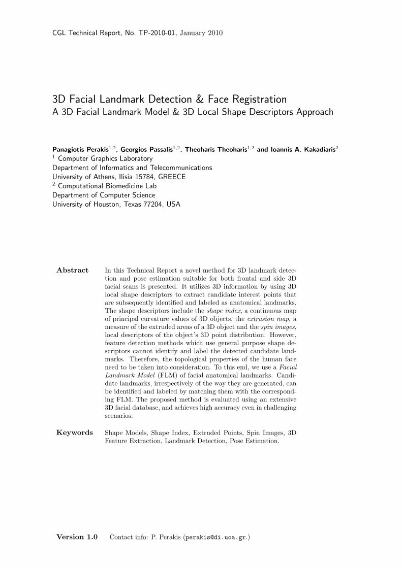
Figure 1: Face registration based on detected landmarks using the proposed method:(a) facial scan with extensive missing data; (b) extracted landmarks; (c) genericReference Face Model (RFM); and (d) registered facial scan with RFM.

Existing 3D feature detection and localization methods, although they claimpose invariance, fail to address large pose variations and to confront the problem ofmissing facial areas in an holistic way (Section 2). The main assumption of thesemethods is that even though the head can be rotated with respect to the sensor, theentire face is always visible. However, this is true only for “almost frontal” scans or“reconstructed” complete face meshes. Side scans usually have large missing areas,due to self-occlusion, that depend on pose variations. These scans are very commonin realistic scenarios such as uncooperative subjects or uncontrolled environments.

The goal of the proposed method is to automatically and pose-invariantly detectlandmarks (eye and mouth corners, nose and chin tips) in any 3D facial scan, andhence consistently register any pair of facial datasets. The main contribution ofour proposed method is its applicability to large pose variations (up to 80◦ of yawrotation), that often result in missing facial data, in an holistic way with high successrates.

2 P. Perakis et al.

At the training phase, our method creates a Facial Landmark Model (FLM) byfirst aligning the training landmark sets and calculating a mean landmark shapeusing Procrustes Analysis, and then applying Principal Component Analysis (PCA)to capture the shape variations. At the detection phase, the algorithm first detectscandidate landmarks on the queried facial datasets exploiting the 3D geometry-basedinformation. The extracted candidate landmarks are then filtered out and labeledby matching them with the FLM. Registration is then performed, based on resultinglandmarks, with a generic Reference Face Model (RFM) (Fig. 1).

Evaluation of the proposed method is performed by computing the distance be-tween manually annotated landmarks (ground truth) and the automatically detectedlandmarks. The experiments have been carried out on a combination of the largestpublicly available databases: FRGC v2 [PFS∗05] and UND Ear Database [UND08].The first is a database for 3D face recognition that contains frontal facial scans,while the second is a database for 3D ear recognition that contains up to 80◦ sidefacial scans (both left and right).

In previous work, we have presented methods for detecting landmarks on 3Dfacial scans. In [PTPK09] shape index and spin images were introduced to locatelandmarks in a manner that allows consistent retrieval of facial regions from 3Dfacial datasets. In [PPT∗09] shape index and extrusion maps were introduced tolocate landmarks for registering partial facial datasets in a face recognition system.

This report describes in detail and extends our previous methods by utilizingstatistically trained spin image templates and alternative similarity distance mea-sures. It achieves significantly higher landmark detection rates, which result in afar more robust face registration. It also contains exhaustive comparative analyti-cal results for landmark localization success rates for all of our methods and otherexisting methods (Tables 8 and 9).

The rest of this report is organized as follows: Section 2 describes related work inthe field, Sections 3 and 4 present the proposed method in detail, Section 5 presentsour results, while Section 6 summarizes our method and proposes future directions.

2 Related Work

Facial feature detectors can be distinguished into two main categories: detection offeature points (landmarks) from the geometric characteristics of 2D intensity or colorimages and detection of feature points (landmarks) from the geometric informationof 3D objects or 2.5D scans. Facial feature detectors can also be classified as thosethat are solely dependent on geometric information or those that are supported bytrained statistical feature models. Three-D facial feature extraction has arousedinterest with the increasing development of 3D modeling and digitizing techniquesand is reported in a number of publications.

Lu, Colbry, Stockman and Jain [LJ05, CSJ05, LJ06, LJC06, Col06], in a seriesof publications, presented methods to locate the positions of eye and mouth corners,and nose and chin tips, based on a fusion scheme of shape index [DJ97] on rangemaps and the “cornerness” response [HS88] on intensity maps. They also developeda heuristic method based on cross-profile analysis to locate the nose tip more ro-

Section 2 Related Work 3

bustly. Candidate landmark points were filtered out using a static (non-deformable)statistical model of landmark positions, in contrast to our approach. The 3D featureextraction method presented in [CSJ05] addresses the problem of pose variations ina unified manner, and is tested against a composite database consisting of 953 scansfrom the FRGC database and 160 scan from a proprietary database with frontalscans extended with variations of pose, expressions, occlusions and noise. Theirmultimodal algorithm [LJ05] uses 3D+2D information and is applicable to almost-frontal scans (< 5◦ yaw rotation). It is tested against the FRGC database with946 near frontal scans. The 3D feature extraction method presented in [LJ06] alsoaddresses the problem of pose variations, and is tested against the FRGC databasewith 953 near frontal scans along with their proprietary MSU database consist-ing of 300 multiview scans (0◦,±45◦) from 100 subjects. Results of the methods[LJ05, LJ06, Col06] are presented in Table 8, and of the method [LJ06] in Table 9,for comparison.

Conde et al. [CCRA∗05] introduced a global face registration method by combin-ing clustering techniques over discrete curvature and spin images for the detectionof eye inner corners and nose tip. The method was tested on a proprietary databaseof 51 subjects with 14 captures each (714 scans). Their database consists of scanswith small pose variations (< 15◦ yaw rotation). Although they presented a featurelocalization success rate of 99.66% on frontal scans and 96.08% on side scans, theydo not define what a successful localization is.

Xu et al. [XTWQ06] presented a feature extraction hierarchical scheme to detectthe positions of nose tip and nose ridge. They introduced the “effective energy” no-tion to describe the local distribution of neighboring points and detect the candidatenose tips. Finally, an SVM classifier is used to select the correct nose tips. Althoughit was tested against various databases, no exact localization results were provided.

Lin et al. [LSCH06] introduced a coupled 2D and 3D feature extraction methodto determine the positions of eye sockets by using curvature analysis. The nose tip isconsidered to be the extreme vertex along the normal direction of eye sockets. Themethod was used in an automatic 3D face authentication system, but was tested ononly 27 human faces with various poses and expressions.

Segundo et al. [SQBS07] introduced a face and facial feature detection methodby combining a method for 2D face segmentation on depth images with surface cur-vature information, in order to detect the eye corners, nose tip, nose base, and nosecorners. The method was tested on the FRGC v2 database. Although they claimover 99.7% correct detections, they do not define a correct detection. Additionally,nose and eye corner detection presented problems when the face had a significantpose variation (> 15◦ yaw and roll).

Wei et al. [WLY07] introduced a nose tip and nose bridge localization methodto determine facial pose. The method was based on a Surface Normal Differencealgorithm and shape index estimation, and was used as a preprocessing step in pose-variant systems to determine the pose of the face. They reported an angular errorof the nose tip - nose bridge segment less than 15◦ in 98% of the 2500 datasetsof BU-3DFE facial database, which contains complete frontal facial datasets withcapture range ±45◦.

Mian et al. [MBO07] introduced a heuristic method for nose tip detection. The

4 P. Perakis et al.

method is based on a geometric analysis of the nose ridge contour projected on thex− y plane. It is used as a preprocessing step to cut out and pose correct the facialdata in a face recognition system. However, no clear localization error results werepresented. Additionally, their nose tip detection algorithm has limited applicabilityto near frontal scans (< 15◦ yaw and pitch).

Faltemier et al. [FBF08a] introduced a heuristic method for nose tip detec-tion. The method is a fusion of curvature and shape index analysis and a templatematching algorithm using ICP. The nose tip detector had a localization error lessthan 10 mm in 98.2% of the 4007 facial datasets of FRGC v2 where it was tested.However, no exact localization distance error results were presented. They also in-troduced a method called “Rotated Profile Signatures” [FBF08b], based on profileanalysis, to robustly locate the nose tip in the presence of pose, expression andocclusion variations. Their method was tested against NDOff2007 database whichcontains 7,317 facial scans, 406 frontal and 6,911 in various yaw and pitch angles.They reported a 96% to 100% success rate, with distance error threshold 10 mm,under significant yaw and pitch variations. Although their method achieved highsuccess rate scores, it is a 2D-assisted 3D method since it uses skin segmentation toeliminate outliers, and is limited to the detection of the nose tip only. Finally, noexact localization distance error results were presented.

Dibeklioglu, Salah and Akarun [Dib08, DSA08] presented methods for detectingfacial features on 3D facial datasets to enable pose correction under significant posevariations. They introduced a statistical method to detect facial features, basedon training a model of local features, from the gradient of the depth map. Themethod was tested against the FRGC v1 and the Bosphorus databases, but datawith pose variations were not taken into consideration. They also introduced a nosetip localization and segmentation method using curvature-based heuristic analysis.However, the proposed system shows limited capabilities on facial datasets with yawrotations greater than 45◦. Additionally, even though the Bosphorus database usedconsists of 3,396 facial scans, they are obtained from 81 subjects. Finally, no exactlocalization distance error results were presented.

Yu and Moon [YM08] presented a nose tip and eye inner corners detectionmethod on 3D range maps. The landmark detector is trained from example fa-cial data using a genetic algorithm. The method was applied on 200 almost-frontalscans from FRGC v1 database. However, a limitation of the proposed system isthat it is not applicable to facial datasets with large yaw rotations since it alwaysuses the three aforementioned control points. Results of the method are presentedin Table 8 for comparison reasons.

Romero-Huertas and Pears [RHP08] presented a graph matching approach tolocate the positions of nose tip and inner eye corners. They introduced the “distanceto local plane” notion to describe the local distribution of neighboring points anddetect convex and concave areas of the face. Finally, after the graph matchingalgorithm has eliminated false candidates, the best combination of landmark pointsis selected from the minimum Mahalanobis distance to the trained landmark graphmodel. The method was tested against FRGC v1 (509 scans) and FRGC v2 (3271scans) databases. They reported a success rate of 90% with thresholds for the nosetip at 15 mm, and for the inner eye corners at 12 mm.

Section 3 3D Facial Landmark Models 5

(a) (b)

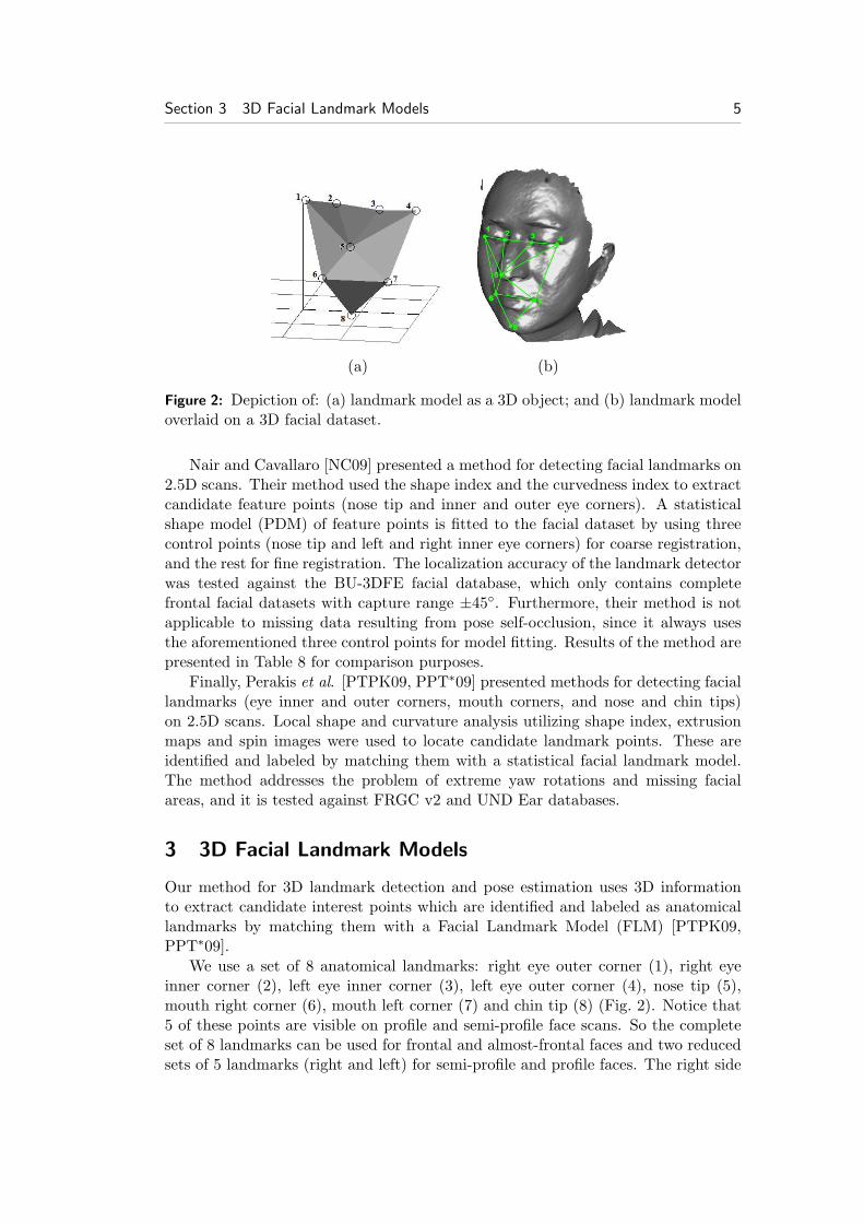
Figure 2: Depiction of: (a) landmark model as a 3D object; and (b) landmark modeloverlaid on a 3D facial dataset.

Nair and Cavallaro [NC09] presented a method for detecting facial landmarks on2.5D scans. Their method used the shape index and the curvedness index to extractcandidate feature points (nose tip and inner and outer eye corners). A statisticalshape model (PDM) of feature points is fitted to the facial dataset by using threecontrol points (nose tip and left and right inner eye corners) for coarse registration,and the rest for fine registration. The localization accuracy of the landmark detectorwas tested against the BU-3DFE facial database, which only contains completefrontal facial datasets with capture range ±45◦. Furthermore, their method is notapplicable to missing data resulting from pose self-occlusion, since it always usesthe aforementioned three control points for model fitting. Results of the method arepresented in Table 8 for comparison purposes.

Finally, Perakis et al. [PTPK09, PPT∗09] presented methods for detecting faciallandmarks (eye inner and outer corners, mouth corners, and nose and chin tips)on 2.5D scans. Local shape and curvature analysis utilizing shape index, extrusionmaps and spin images were used to locate candidate landmark points. These areidentified and labeled by matching them with a statistical facial landmark model.The method addresses the problem of extreme yaw rotations and missing facialareas, and it is tested against FRGC v2 and UND Ear databases.

3 3D Facial Landmark Models

Our method for 3D landmark detection and pose estimation uses 3D informationto extract candidate interest points which are identified and labeled as anatomicallandmarks by matching them with a Facial Landmark Model (FLM) [PTPK09,PPT∗09].

We use a set of 8 anatomical landmarks: right eye outer corner (1), right eyeinner corner (2), left eye inner corner (3), left eye outer corner (4), nose tip (5),mouth right corner (6), mouth left corner (7) and chin tip (8) (Fig. 2). Notice that5 of these points are visible on profile and semi-profile face scans. So the completeset of 8 landmarks can be used for frontal and almost-frontal faces and two reducedsets of 5 landmarks (right and left) for semi-profile and profile faces. The right side

6 P. Perakis et al.

landmark set contains the points (1), (2), (5), (6), and (8), and the left side thepoints (3), (4), (5), (7) and (8).

Each of these sets of landmarks constitute a corresponding Facial LandmarkModel (FLM). In the following, the model of the complete set of eight landmarkswill be referred to as FLM8 and the two reduced sets of five landmarks (left andright) as FLM5L and FLM5R, respectively. The main steps to create the FLMs are:

• A statistical mean shape for each landmark set (FLM8, FLM5L and FLM5R)is calculated from a manually annotated training set using Procrustes Analysis.One hundred and fifty frontal face scans with neutral expressions are randomlychosen from the FRGC v2 database as our training examples.

• Variations of each Facial Landmark Model are calculated using Principal Com-ponent Analysis (PCA).

3.1 The Landmark Mean Shape

According to Dryden and Mardia [DM98], “a landmark is a point of correspondenceon each object that matches between and within populations of the same class ofobjects” and “a shape is all the geometrical information that remains when location,scale and rotational effects are filtered out from an object”. Shape, in other words,is invariant to Euclidean similarity transformations.

Since, for our purposes, the size of the shape is of great importance, it is notfiltered out by scaling shapes to unit size. So, “two objects have the same size-and-shape if they are rigid-body transformations of each other” [DM98].

One way to describe a shape is by locating a finite number of landmarks on theoutline or other specific points. Dryden and Mardia [DM98] sort landmarks into thefollowing categories:

Anatomical landmarks: Points assigned by an expert that correspond betweenorganisms in some biologically meaningful way (e.g., the corner of an eye).

Mathematical landmarks: Points located on an object according to some mathe-matical or geometrical property (e.g., a high curvature or an extremum point).

Pseudo-landmarks: Constructed points on an object either on the outline orbetween anatomical or mathematical landmarks.

Labeled landmarks: Landmarks that are associated with a label (name or num-ber), which is used to identify the corresponding landmark.

Synonyms for landmarks include homologous points, interest points, nodes, ver-tices, anchor points, fiducial markers, model points, markers, key points, etc.

A mathematical representation of an n-point shape in d dimensions can be de-fined by concatenating all point coordinates into a k = n×d vector and establishinga Shape Space [DM98, SG02, CT01]. The vector representation for 3D shapes (i.e.,d = 3) would then be:

x = [x1, x2, ..., xn, y1, y2, ..., yn, z1, z2, ..., zn]T (1)


where (xi, yi, zi) represent the n landmark points.To obtain a true representation of landmark shapes, location and rotational ef-

fects need to be filtered out. This is carried out by establishing a common coordinatereference to which all shapes are aligned.

Alignment is performed by minimizing the Procrustes distance

D2P = |xi − xm|2 =

k∑j=1

(xij − xmj)2 (2)

of each shape xi to the mean shape xm.The alignment procedure is commonly known as Procrustes Analysis [DM98,

SG02, CT01] and is used to calculate the mean shape of landmark shapes. Al-though there are analytic solutions, a typical iterative approach,adapted from [CT01], is the following:

Algorithm 1: Procrustes Analysis

• Compute the centroid of each example shape.

• Translate each example shape so that its centroid is at the origin (0,0,0).

• Scale each example shape so that its size is 1.

• Assign the first example shape to the mean shape xm.

• REPEAT

– Assign the mean shape xm to a reference mean shape x0.

– Align all example shapes to the reference mean shape x0 by an optimalrotation.

– Recalculate the mean shape xm.

– Translate the mean shape so that its centroid is at the origin (0,0,0).

– Scale the mean shape so that its its size is 1.

– Align the mean shape xm to the reference mean shape x0 by an optimalrotation.

– Compute the Procrustes distance of the mean shape xm to the referencemean shape x0:|x0 − xm|.

• UNTIL Convergence: |x0 − xm| < ε.

In our case, where the size of the facial landmark shape is of great importance,scaling shapes to unit size is omitted. In these cases, shapes are considered rigidshapes and are aligned by performing only the translational and rotational transfor-mations.

Thus the mean shape of landmark shapes (Fig. 3) is created and example shapesare aligned to the mean shape.

The mean shape xm is the Procrustes mean

xm =1N

N∑i=1

xi (3)

8 P. Perakis et al.

(a) (b) (c) (d)

Figure 3: Depiction of landmarks mean shape estimation: (a) unaligned landmarks;(b) aligned landmarks; (c) landmarks mean shape; and (d) landmark cloud andmean shape at 60o.

of all N example shapes xi.

3.2 Shape Alignment Transformations

As we have previously mentioned, to obtain a true representation of landmarkshapes, location, scale and rotational effects need to be filtered out by bringingshapes to a common frame of reference. This is carried out by performing transla-tional, scaling and rotational transformations. Notice that different approaches toalignment can produce different distributions of the aligned shapes.

Translation to the centroid is performed by applying to the n landmark pointsrj the following transformation in 3D original space:

r′j = rj − rc (4)

where rc the centroid and j ∈ {1, ..., n}.The centroid of a shape is the center of mass (CM) of the physical system con-

sisting of unit masses at each landmark. This is easily calculated as:

rc =

1n

n∑j=1

xj ,1n

n∑j=1

yj ,1n

n∑j=1

zj

T (5)

in a 3D original space (i.e., d = 3).Scaling to unit size is performed by applying to the landmark points rj the

following transformation in 3D original space:

r′j = αrj (6)

where α = 1/S(x) is the scaling factor, S(x) is the shape’s size, and j ∈ {1, ..., n}.The shape’s size is the square root of the sum of squared Euclidean distances

from each landmark rj to the centroid rc:

S(x)2 =n∑j=1

|rj − rc|2 (7)

in the original 3D space.


Rotation in the original 3D space is slightly more complicated. We must cal-culate a rotational transformation R(x) so as to minimize the Procrustes distance|R(x)− x0| of the transformed shape R(x) to a reference shape x0. The rotationaltransformation R can be expressed as a product of three rotations around the threeprincipal axes:

R = Rx,θ ·Ry,φ ·Rz,ψ (8)

These can be expressed in a matrix form:

Rx,θ =

1 0 00 cos θ − sin θ0 sin θ cos θ

(9)

Ry,φ =

cosφ 0 sinφ0 1 0

− sinφ 0 cosφ

(10)

Rz,ψ =

cosψ − sinψ 0sinψ cosψ 0

0 0 1

(11)

After setting partial derivatives of |R(x)−x0|2 w.r.t each parameter to zero andsome formal calculations, we have:

θ = tan−1

(Sz0,y − Sy0,zSy0,y + Sz0,z

)(12)

φ = tan−1

(Sx0,z − Sz0,xSz0,z + Sx0,x

)(13)

ψ = tan−1

(Sy0,x − Sx0,ySx0,x + Sy0,y

)(14)

where:

Sx0,x =∑n

j=1 x0jxj , Sx0,y =∑n

j=1 x0jyj , Sx0,z =∑n

j=1 x0jzj ,

Sy0,x =∑n

j=1 y0jxj , Sy0,y =∑n

j=1 y0jyj , Sy0,z =∑n

j=1 y0jzj ,

Sz0,x =∑n

j=1 z0jxj , Sz0,y =∑n

j=1 z0jyj , Sz0,z =∑n

j=1 z0jzj .

So, the rotational transformation of every landmark point rj in the original 3Dspace gives:

rj′ = R(rj) = Rx,θ (Ry,φ (Rz,ψ(rj))) (15)

Alignment of a shape x to a reference shape x0 is done by minimizing the Pro-crustes distance in an iterative way, as described below:

10 P. Perakis et al.

Algorithm 2: Shape Alignment

• Translate x0 so that its centroid is at the origin (0,0,0).

• Scale x0 so that its size is 1.

• Translate x so that its centroid is at the origin (0,0,0).

• Scale x so that its size is 1.

• Set R← I.

• REPEAT

– Calculate Rx,θ.

– Apply Rx,θ to x shape points.

– Set R← Rx,θ ·R.

– Calculate Ry,φ.

– Apply Ry,φ to x shape points.

– Set R← Ry,φ ·R.

– Calculate Rz,ψ.

– Apply Rz,ψ to x shape points.

– Set R← Rz,ψ ·R.

– Compute the Procrustes distance of the transformed shape x to thereference shape x0:|x0 − x|.

• UNTIL Convergence: |x− x0| < ε.

• Get R.

Note that, in our case, where the size of the facial landmark shape is of greatimportance, scaling shapes to unit size is omitted. Also note that the proposed“Shape Alignment” algorithm leaves us the discretion to permit certain rotations(e.g., only around the y-axis).

3.3 Landmark Shape Variations

After bringing landmark shapes into a common frame of reference and estimatingthe landmarks’ mean shape, further analysis can be carried out for describing theshape variations. This shape decomposition is performed by applying PrincipalComponent Analysis (PCA) to the aligned shapes.

Due to size normalization of Procrustes analysis, all shape vectors live in a hypersphere manifold in shape space, which introduces non-linearities if large shape scal-ings occur. Since PCA is a linear procedure, all aligned shapes are at first projectedto the tangent space of the mean shape. This way, shape vectors lie in a hyper planeinstead of a hyper sphere, and non-linearities are filtered out. The tangent spaceprojection linearizes shapes by scaling them with a factor α:

xt = αx =|xm|2

xm · xx (16)


where xt is the tangent space projection of shape x and xm is the mean shape.If no size normalization is applied, then tangent space projection can be omitted.Aligned shape vectors form a distribution in the nd dimensional shape space,

where n is the number of landmarks and d the dimension of each landmark. Iflandmark points are not representing a certain class of shapes, then they will betotally uncorrelated (i.e., purely random). On the other hand, if landmark pointsrepresent a certain class of shapes, then they will be correlated to some degree. Thisfact will be exploited by applying PCA to reduce dimensionality and obtain thecorrelation as deformations.

If landmark points have a specific distribution, we can model this distribu-tion by estimating a vector b of parameters that describes a shape’s deformations[CTCG95, CT01, CTKP05, SG02]. The approach is as follows:

Algorithm 3: Principal Component Analysis

• Determine the mean shape.

• Determine the covariance matrix of the shape vectors.

• Compute the eigenvectors Ai and corresponding eigenvalues λi of the covari-ance matrix, sorted in descending order.

After applying Procrustes analysis, the mean shape is determined and exampleshapes are aligned and projected to the mean shape’s tangent space. Typically, onewould apply PCA on variables with zero mean.

The covariance matrix of N example shapes is calculated according to

Cx =1

N − 1

N∑i=1

(xi − xm)(xi − xm)T (17)

If A contains (in columns) the k = nd eigenvectors Ai of Cx, by projectingaligned original example shapes to the eigenspace we uncorrelate them as

y = AT · (x− xm) (18)

and the covariance matrix of projected example shapes

Cy =1

N − 1

N∑i=1

(yi − ym)(yi − ym)T (19)

becomes a diagonal matrix of the eigenvalues λi, so as to have

Cx ·A = A ·Cy , Cy = AT ·Cx ·A (20)

The resulting transform is known as the Karhunen-Loeve transform, and achievesour original goal of creating mutually uncorrelated features.

To back-project uncorrelated shape vectors into the original shape space, we canuse

x = xm + A · y (21)


(a)b1 = −3

√λ1

(b)b1 = 0

(c)b1 = +3

√λ1

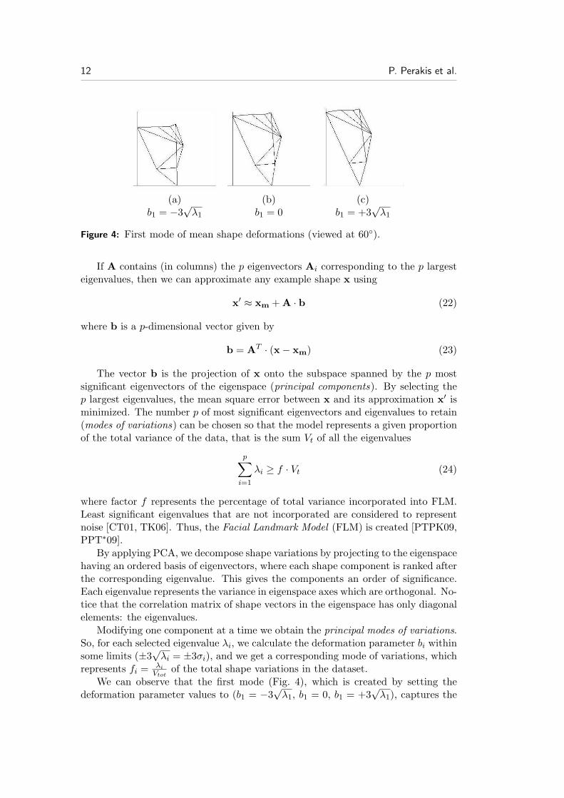
Figure 4: First mode of mean shape deformations (viewed at 60◦).

If A contains (in columns) the p eigenvectors Ai corresponding to the p largesteigenvalues, then we can approximate any example shape x using

x′ ≈ xm + A · b (22)

where b is a p-dimensional vector given by

b = AT · (x− xm) (23)

The vector b is the projection of x onto the subspace spanned by the p mostsignificant eigenvectors of the eigenspace (principal components). By selecting thep largest eigenvalues, the mean square error between x and its approximation x′ isminimized. The number p of most significant eigenvectors and eigenvalues to retain(modes of variations) can be chosen so that the model represents a given proportionof the total variance of the data, that is the sum Vt of all the eigenvalues

p∑i=1

λi ≥ f · Vt (24)

where factor f represents the percentage of total variance incorporated into FLM.Least significant eigenvalues that are not incorporated are considered to representnoise [CT01, TK06]. Thus, the Facial Landmark Model (FLM) is created [PTPK09,PPT∗09].

By applying PCA, we decompose shape variations by projecting to the eigenspacehaving an ordered basis of eigenvectors, where each shape component is ranked afterthe corresponding eigenvalue. This gives the components an order of significance.Each eigenvalue represents the variance in eigenspace axes which are orthogonal. No-tice that the correlation matrix of shape vectors in the eigenspace has only diagonalelements: the eigenvalues.

Modifying one component at a time we obtain the principal modes of variations.So, for each selected eigenvalue λi, we calculate the deformation parameter bi withinsome limits (±3

√λi = ±3σi), and we get a corresponding mode of variations, which

represents fi = λiVtot

of the total shape variations in the dataset.We can observe that the first mode (Fig. 4), which is created by setting the

deformation parameter values to (b1 = −3√λ1, b1 = 0, b1 = +3

√λ1), captures the


(a)b2 = −3

√λ2

(b)b2 = 0

(c)b2 = +3

√λ2

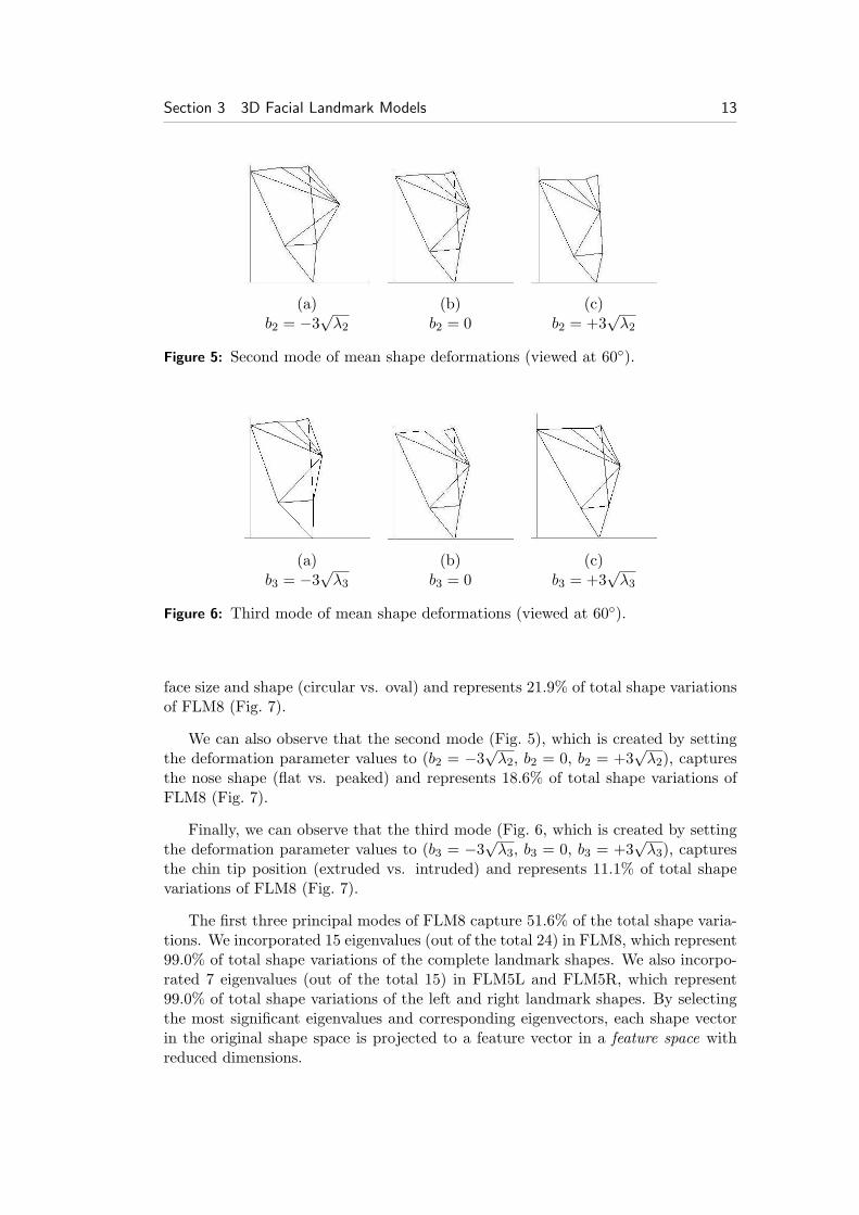
Figure 5: Second mode of mean shape deformations (viewed at 60◦).

(a)b3 = −3

√λ3

(b)b3 = 0

(c)b3 = +3

√λ3

Figure 6: Third mode of mean shape deformations (viewed at 60◦).

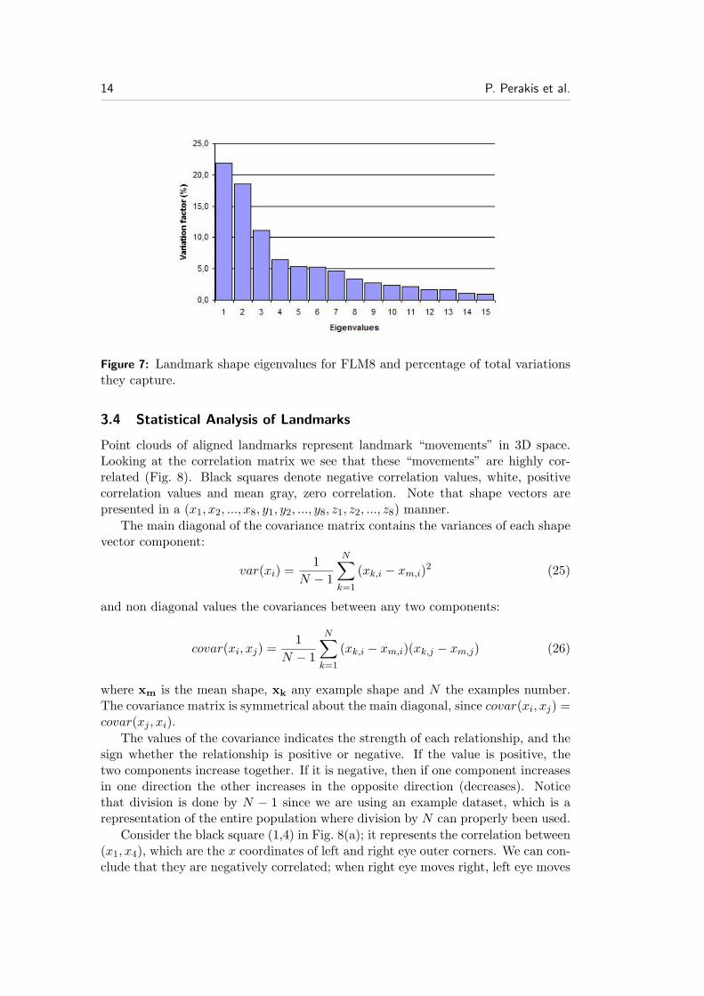
face size and shape (circular vs. oval) and represents 21.9% of total shape variationsof FLM8 (Fig. 7).

We can also observe that the second mode (Fig. 5), which is created by settingthe deformation parameter values to (b2 = −3

√λ2, b2 = 0, b2 = +3

√λ2), captures

the nose shape (flat vs. peaked) and represents 18.6% of total shape variations ofFLM8 (Fig. 7).

Finally, we can observe that the third mode (Fig. 6, which is created by settingthe deformation parameter values to (b3 = −3

√λ3, b3 = 0, b3 = +3

√λ3), captures

the chin tip position (extruded vs. intruded) and represents 11.1% of total shapevariations of FLM8 (Fig. 7).

The first three principal modes of FLM8 capture 51.6% of the total shape varia-tions. We incorporated 15 eigenvalues (out of the total 24) in FLM8, which represent99.0% of total shape variations of the complete landmark shapes. We also incorpo-rated 7 eigenvalues (out of the total 15) in FLM5L and FLM5R, which represent99.0% of total shape variations of the left and right landmark shapes. By selectingthe most significant eigenvalues and corresponding eigenvectors, each shape vectorin the original shape space is projected to a feature vector in a feature space withreduced dimensions.


Figure 7: Landmark shape eigenvalues for FLM8 and percentage of total variationsthey capture.

3.4 Statistical Analysis of Landmarks

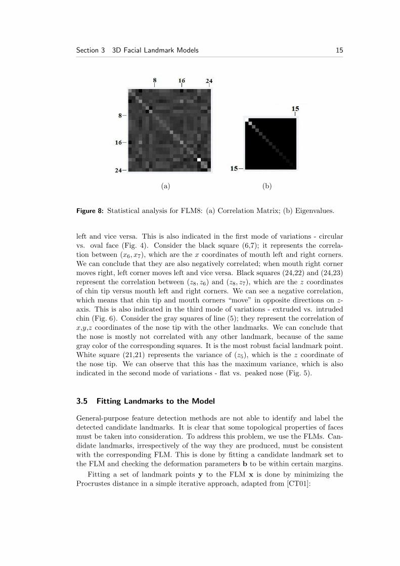
Point clouds of aligned landmarks represent landmark “movements” in 3D space.Looking at the correlation matrix we see that these “movements” are highly cor-related (Fig. 8). Black squares denote negative correlation values, white, positivecorrelation values and mean gray, zero correlation. Note that shape vectors arepresented in a (x1, x2, ..., x8, y1, y2, ..., y8, z1, z2, ..., z8) manner.

The main diagonal of the covariance matrix contains the variances of each shapevector component:

var(xi) =1

N − 1

N∑k=1

(xk,i − xm,i)2 (25)

and non diagonal values the covariances between any two components:

covar(xi, xj) =1

N − 1

N∑k=1

(xk,i − xm,i)(xk,j − xm,j) (26)

where xm is the mean shape, xk any example shape and N the examples number.The covariance matrix is symmetrical about the main diagonal, since covar(xi, xj) =covar(xj , xi).

The values of the covariance indicates the strength of each relationship, and thesign whether the relationship is positive or negative. If the value is positive, thetwo components increase together. If it is negative, then if one component increasesin one direction the other increases in the opposite direction (decreases). Noticethat division is done by N − 1 since we are using an example dataset, which is arepresentation of the entire population where division by N can properly been used.

Consider the black square (1,4) in Fig. 8(a); it represents the correlation between(x1, x4), which are the x coordinates of left and right eye outer corners. We can con-clude that they are negatively correlated; when right eye moves right, left eye moves


(a) (b)

Figure 8: Statistical analysis for FLM8: (a) Correlation Matrix; (b) Eigenvalues.

left and vice versa. This is also indicated in the first mode of variations - circularvs. oval face (Fig. 4). Consider the black square (6,7); it represents the correla-tion between (x6, x7), which are the x coordinates of mouth left and right corners.We can conclude that they are also negatively correlated; when mouth right cornermoves right, left corner moves left and vice versa. Black squares (24,22) and (24,23)represent the correlation between (z8, z6) and (z8, z7), which are the z coordinatesof chin tip versus mouth left and right corners. We can see a negative correlation,which means that chin tip and mouth corners “move” in opposite directions on z-axis. This is also indicated in the third mode of variations - extruded vs. intrudedchin (Fig. 6). Consider the gray squares of line (5); they represent the correlation ofx,y,z coordinates of the nose tip with the other landmarks. We can conclude thatthe nose is mostly not correlated with any other landmark, because of the samegray color of the corresponding squares. It is the most robust facial landmark point.White square (21,21) represents the variance of (z5), which is the z coordinate ofthe nose tip. We can observe that this has the maximum variance, which is alsoindicated in the second mode of variations - flat vs. peaked nose (Fig. 5).

3.5 Fitting Landmarks to the Model

General-purpose feature detection methods are not able to identify and label thedetected candidate landmarks. It is clear that some topological properties of facesmust be taken into consideration. To address this problem, we use the FLMs. Can-didate landmarks, irrespectively of the way they are produced, must be consistentwith the corresponding FLM. This is done by fitting a candidate landmark set tothe FLM and checking the deformation parameters b to be within certain margins.

Fitting a set of landmark points y to the FLM x is done by minimizing theProcrustes distance in a simple iterative approach, adapted from [CT01]:


Algorithm 4: Landmark Fitting

• Translate y so that its centroid is at the origin (0,0,0).

• Scale y shape so that its size is 1.

• REPEAT

– Align y to the mean shape xm by an optimal rotation.

– Compute the Procrustes distance of y to the mean shape xm: |y−xm|.

• UNTIL Convergence: |y − xm| < ε.

• Project y into tangent space of xm.

• Determine the model deformation parameters b that match to y:b = AT · (y − xm).

• Accept y as a member of the shape’s class if b satisfies certain constraints.

Notice that scaling is not applied when we need to retain shape size.We consider a landmark shape as plausible if it is consistent with marginal shape

deformations. Let us say that certain bi satisfy the deformation constraint

|bi| ≤ 3√λi (27)

then the candidate landmark shape belongs to the shape class with probabilityPr(y):

Pr(y) =∑λi

Vp(28)

where λi are the eigenvalues that satisfy the deformation constraints and Vp is thesum of the eigenvalues that correspond to the selected p principal components, andrepresents the incorporated data variance.

If Pr(y) exceeds a certain threshold limit, the landmark shape is consideredplausible, otherwise it is rejected as a member of the class. Other criteria of declaringa shape as plausible can also be applied [CT01, CTKP05].

4 Landmark Detection & Labeling

To detect landmark points, we have used three 3D local shape descriptors thatexploit the 3D geometry-based information of facial datasets: shape index, extrusionmap and spin images.

A facial scan belongs to a subclass of 3D objects which can be considered as asurface S expressed in a general parametric form w.r.t. a known coordinate system:

S(p) = {p ∈ R3 : p = [x(u, v), y(u, v), z(u, v)]T , (u, v) ∈ R2} (29)

This global native u, v parameterization of the facial scan allows us to map 3Dinformation into 2D space. Since differential geometry is used for describing localbehavior of surfaces in a small neighborhood, such as surface curvature and surfacenormals, we assume that the surface S can be adequately modeled as being at least

Section 4 Landmark Detection & Labeling 17

piecewise smooth, that is at least be of class C2 (twice differentiable). Therefore,to eliminate sensor-specific problems, certain preprocessing algorithms (median cut,hole filling, smoothing, and subsampling) operate directly on the range data beforethe conversion to polygonal data [KPT∗07].

4.1 Shape Index

The Shape Index is extensively used for 3D landmark detection [Col06, LJ06, LJC06,CSJ05, LJ05]. It is a continuous mapping of principal curvature values (kmax, kmin)of a 3D object point p into the interval [0,1], according to the formula:

SI(p) =12− 1πtan−1kmax(p) + kmin(p)

kmax(p)− kmin(p)(30)

We use the Dorai and Jain definition here [DJ97], an extension of Koenderinkand van Doorn’s original definition [KvD92]. The shape index captures the intuitivenotion of “local” shape of a surface. Every distinct surface shape corresponds to aunique value of shape index, except the planar shape. Points on a planar surfacehave an indeterminate shape index, since kmax = kmin = 0. Five well-known shapetypes and their locations on the shape index scale are as follows: Cup = 0.0, Rut =0.25, Saddle = 0.5, Ridge = 0.75, and Cap = 1.0.

After calculating shape index values on a 3D facial dataset, a mapping to 2Dspace is performed (using the native u, v parameterization of the facial scan) in orderto create a shape index map (Fig. 9):

SImap(u, v)← ShapeIndex(x, y, z) (31)

Local maxima and minima are identified on the shape index map. Local maxima(SImap(u, v) → 1.0) are candidate landmarks for nose tips and chin tips and localminima (SImap(u, v) → 0.0) for eye corners and mouth corners. The shape index’smaxima and minima that are located are sorted in descending order of significanceaccording to their corresponding shape index values. The most significant subset ofpoints for each group (Caps and Cups) is retained (a maximum of 512 Caps and 512Cups). In Fig. 15(a) and Fig. 16(a), black boxes represent Caps, and white boxesCups.

However, experimentation showed that the shape index alone is not sufficientlyrobust for detecting anatomical landmarks in facial datasets in a variety of poses.Thus, candidate landmarks estimated from shape index values serve as a basis, butmust be further classified and filtered according to the following methods.

4.2 Extruded points

Our experiments indicated that the shape index is not sufficiently robust for detect-ing the nose and chin tips. Thus, we propose a novel method based on two commonattributes for locating these two landmarks. The first attribute is that they extrudefrom the rest of the face. To encode this feature we use the radial map (Fig. 10(a)).


(a) (b) (c)

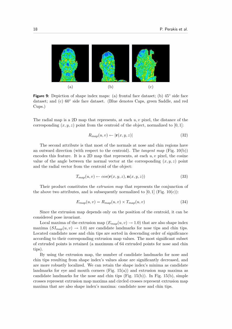
Figure 9: Depiction of shape index maps: (a) frontal face dataset; (b) 45◦ side facedataset; and (c) 60◦ side face dataset. (Blue denotes Caps, green Saddle, and redCups.)

The radial map is a 2D map that represents, at each u, v pixel, the distance of thecorresponding (x, y, z) point from the centroid of the object, normalized to [0, 1]:

Rmap(u, v)← |r(x, y, z)| (32)

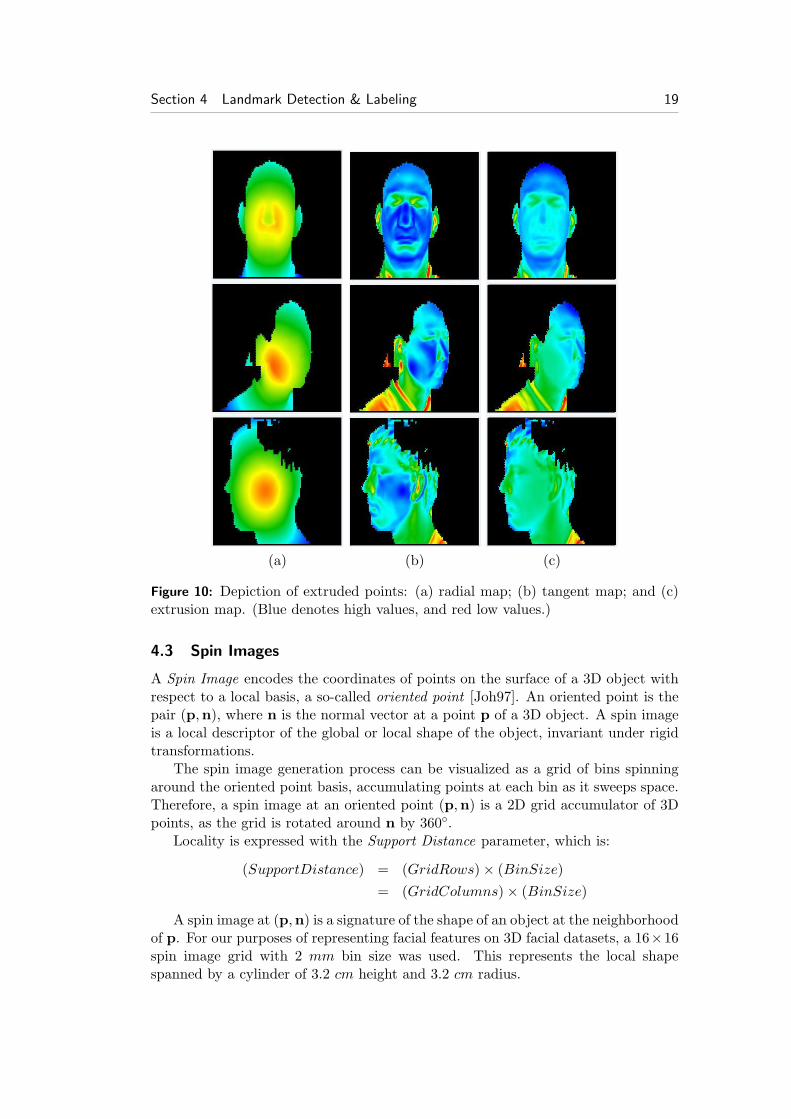
The second attribute is that most of the normals at nose and chin regions havean outward direction (with respect to the centroid). The tangent map (Fig. 10(b))encodes this feature. It is a 2D map that represents, at each u, v pixel, the cosinevalue of the angle between the normal vector at the corresponding (x, y, z) pointand the radial vector from the centroid of the object:

Tmap(u, v)← cos(r(x, y, z),n(x, y, z)) (33)

Their product constitutes the extrusion map that represents the conjunction ofthe above two attributes, and is subsequently normalized to [0, 1] (Fig. 10(c)):

Emap(u, v) = Rmap(u, v)× Tmap(u, v) (34)

Since the extrusion map depends only on the position of the centroid, it can beconsidered pose invariant.

Local maxima of the extrusion map (Emap(u, v)→ 1.0) that are also shape indexmaxima (SImap(u, v) → 1.0) are candidate landmarks for nose tips and chin tips.Located candidate nose and chin tips are sorted in descending order of significanceaccording to their corresponding extrusion map values. The most significant subsetof extruded points is retained (a maximum of 64 extruded points for nose and chintips).

By using the extrusion map, the number of candidate landmarks for nose andchin tips resulting from shape index’s values alone are significantly decreased, andare more robustly localized. We can retain the shape index’s minima as candidatelandmarks for eye and mouth corners (Fig. 15(a)) and extrusion map maxima ascandidate landmarks for the nose and chin tips (Fig. 15(b)). In Fig. 15(b), simplecrosses represent extrusion map maxima and circled crosses represent extrusion mapmaxima that are also shape index’s maxima: candidate nose and chin tips.


(a) (b) (c)

Figure 10: Depiction of extruded points: (a) radial map; (b) tangent map; and (c)extrusion map. (Blue denotes high values, and red low values.)

4.3 Spin Images

A Spin Image encodes the coordinates of points on the surface of a 3D object withrespect to a local basis, a so-called oriented point [Joh97]. An oriented point is thepair (p,n), where n is the normal vector at a point p of a 3D object. A spin imageis a local descriptor of the global or local shape of the object, invariant under rigidtransformations.

The spin image generation process can be visualized as a grid of bins spinningaround the oriented point basis, accumulating points at each bin as it sweeps space.Therefore, a spin image at an oriented point (p,n) is a 2D grid accumulator of 3Dpoints, as the grid is rotated around n by 360◦.

Locality is expressed with the Support Distance parameter, which is:

(SupportDistance) = (GridRows)× (BinSize)= (GridColumns)× (BinSize)

A spin image at (p,n) is a signature of the shape of an object at the neighborhoodof p. For our purposes of representing facial features on 3D facial datasets, a 16×16spin image grid with 2 mm bin size was used. This represents the local shapespanned by a cylinder of 3.2 cm height and 3.2 cm radius.


(a) (b) (c) (d) (e)

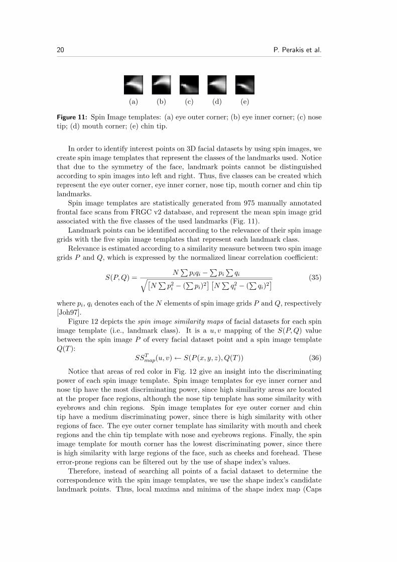
Figure 11: Spin Image templates: (a) eye outer corner; (b) eye inner corner; (c) nosetip; (d) mouth corner; (e) chin tip.

In order to identify interest points on 3D facial datasets by using spin images, wecreate spin image templates that represent the classes of the landmarks used. Noticethat due to the symmetry of the face, landmark points cannot be distinguishedaccording to spin images into left and right. Thus, five classes can be created whichrepresent the eye outer corner, eye inner corner, nose tip, mouth corner and chin tiplandmarks.

Spin image templates are statistically generated from 975 manually annotatedfrontal face scans from FRGC v2 database, and represent the mean spin image gridassociated with the five classes of the used landmarks (Fig. 11).

Landmark points can be identified according to the relevance of their spin imagegrids with the five spin image templates that represent each landmark class.

Relevance is estimated according to a similarity measure between two spin imagegrids P and Q, which is expressed by the normalized linear correlation coefficient:

S(P,Q) =N∑piqi −

∑pi∑qi√[

N∑p2i − (

∑pi)2

] [N∑q2i − (

∑qi)2] (35)

where pi, qi denotes each of the N elements of spin image grids P and Q, respectively[Joh97].

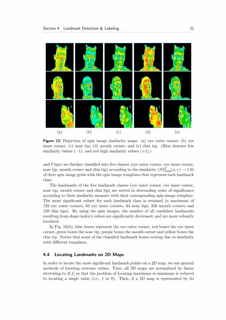
Figure 12 depicts the spin image similarity maps of facial datasets for each spinimage template (i.e., landmark class). It is a u, v mapping of the S(P,Q) valuebetween the spin image P of every facial dataset point and a spin image templateQ(T ):

SSTmap(u, v)← S(P (x, y, z), Q(T )) (36)

Notice that areas of red color in Fig. 12 give an insight into the discriminatingpower of each spin image template. Spin image templates for eye inner corner andnose tip have the most discriminating power, since high similarity areas are locatedat the proper face regions, although the nose tip template has some similarity witheyebrows and chin regions. Spin image templates for eye outer corner and chintip have a medium discriminating power, since there is high similarity with otherregions of face. The eye outer corner template has similarity with mouth and cheekregions and the chin tip template with nose and eyebrows regions. Finally, the spinimage template for mouth corner has the lowest discriminating power, since thereis high similarity with large regions of the face, such as cheeks and forehead. Theseerror-prone regions can be filtered out by the use of shape index’s values.

Therefore, instead of searching all points of a facial dataset to determine thecorrespondence with the spin image templates, we use the shape index’s candidatelandmark points. Thus, local maxima and minima of the shape index map (Caps


(a) (b) (c) (d) (e)

Figure 12: Depiction of spin image similarity maps: (a) eye outer corner; (b) eyeinner corner; (c) nose tip; (d) mouth corner; and (e) chin tip. (Blue denotes lowsimilarity values (−1), and red high similarity values (+1).)

and Cups) are further classified into five classes (eye outer corner, eye inner corner,nose tip, mouth corner and chin tip) according to the similarity (SSTmap(u, v)→ 1.0)of their spin image grids with the spin image templates that represent each landmarkclass.

The landmarks of the five landmark classes (eye outer corner, eye inner corner,nose tip, mouth corner and chin tip) are sorted in descending order of significanceaccording to their similarity measure with their corresponding spin image template.The most significant subset for each landmark class is retained (a maximum of128 eye outer corners, 64 eye inner corners, 64 nose tips, 256 mouth corners and128 chin tips). By using the spin images, the number of all candidate landmarksresulting from shape index’s values are significantly decreased, and are more robustlylocalized.

In Fig. 16(b), blue boxes represent the eye outer corner, red boxes the eye innercorner, green boxes the nose tip, purple boxes the mouth corner and yellow boxes thechin tip. Notice that some of the classified landmark boxes overlap due to similaritywith different templates.

4.4 Locating Landmarks on 2D Maps

In order to locate the most significant landmark points on a 2D map, we use generalmethods of locating extreme values. First, all 2D maps are normalized by linearstretching to [0,1] so that the problem of locating maximum or minimum is reducedto locating a single value (i.e., 1 or 0). Then, if a 2D map is represented by its


values I(u, v) and a target value V is searched within it, we can consider the function|I(u, v)− V | as a transformation of the 2D map and search for its minimum values.

The localization of target values on a 2D map can be implemented by the algo-rithm below:

Algorithm 5: Landmark Localization

• FOR each point (u, v).

– Calculate |I(u, v)− V |.– IF |I(u, v)− V | > V ar reject point (u, v).

– IF |I(u, v)−V | is not a minimum in a window of neighbors reject point(u, v).

– IF |I(u, v)−V | is not a majority value in a window of neighbors rejectpoint (u, v).

– IF NOT rejected add point in a descending ordered list of points ac-cording to |I(u, v)− V |.

• END FOR.

• Return list of points.

The algorithm calculates the value |I(u, v) − V | and tests if it is within certainaccepted variation limits V ar in order to reject unwanted values (outliers). Then ittests if |I(u, v)−V | is a local minimum within a window of neighbors by suppressingnon minimum candidate points (hill climbing scheme). Finally, it tests wether thetarget value is a majority value (within some limits |I(u, v)−V | ≤ V ar) in a windowof neighbors (voting scheme). Thus a list of points is returned, sorted in descendingorder of significance, according to the distance from target value |I(u, v)− V |.

4.5 Landmark Labeling & Selection

As we have previously mentioned, detected geometric landmarks must be identifiedand labeled as anatomical landmarks. For this purpose, topological properties offaces must be taken into consideration. Thus, candidate geometric landmarks, irre-spectively of the way they are produced, must be consistent with the FLMs. Thisis done by applying the fitting procedure as described in Section 3.5.

For each facial dataset, the procedure for landmark detection and labeling hasthe following steps:

1. Extract candidate landmarks from the geometric properties of the facial scans.

2. Create feasible combinations of 5 landmarks from the candidate landmark points.

3. Compute the rigid transformation that best aligns the combinations of five candidatelandmarks with the FLM5R and FLM5L.

4. Filter out those combinations that are not consistent with FLM5L or FLM5R, byapplying the fitting procedure as previously described.

5. Sort consistent right (FLM5R) and left (FLM5L) landmark sets in descending orderaccording to a distance metric from the corresponding FLM.


6. Fuse accepted combinations of 5 landmarks (left and right) in complete landmark setsof 8 landmarks.

7. Compute the rigid transformation that best aligns the combinations of eight landmarkswith the FLM8.

8. Discard combinations of landmarks that are not consistent with the FLM8, by apply-ing the fitting procedure as previously described.

9. Sort consistent complete landmark sets in descending order according to a distancemetric from the FLM8.

10. Select the best combination of landmarks (consistent with FLM5R, FLM5R or FLM8)based on the distance metric to the corresponding FLM.

11. Obtain the corresponding rigid transformation for registration.

In Fig. 15(c) and Fig. 16(c), blue boxes represent landmark sets consistent withthe FLM5R, red boxes with the FLM5L, green boxes with the FLM8, and yellowboxes the best landmark set. Notice that some of the consistent landmarks overlap.Also note that the FLM8 consistent landmark set is not always the best solution;FLM5L and FLM5R are usually better solutions for side facial datasets (Fig. 15(d)and Fig. 16(d)).

The consistent landmark sets determine the pose of the face object under con-sideration from the alignment transformation with the corresponding FLM. Sinceour aim is to locate landmark sets on profile, semi-profile and profile faces, we re-tain the complete landmark solution only if estimated yaw-angle is within certainlimits (±30◦ around y-axis), otherwise the left or right landmark sets are preferredaccording to pose.

Finally, using the selected best solution, the registration transformation is calcu-lated, the yaw-angle is estimated, and the facial dataset is classified as frontal, leftside or right side.

Note that the use of landmark sets of 5 landmarks serves two purposes: (i) itis the potential solution for semi-profile and profile faces, and (ii) it reduces thecombinatory search space for creating the complete landmark sets in a divide-and-conquer manner. Instead of creating 8-tuples of landmarks out of N candidates,which generates N8 combinations to be checked for consistency with the FLMs, wecreate 5-tuples of landmarks, and check N5+N5 = 2N5 combinations for consistencywith FLM5L and FLM5R. We retain 256 landmark sets consistent with FLM5L and256 landmark sets consistent with FLM5R. By fusing them and checking consistencywith FLM8 we have an extra of 256×256 combinations to be checked. Thus, by thisapproach 2N5 + 2562 � N8 combinations are checked, with O(N5) � O(N8). ForN = 128 we have approx. 69× 109 instead of 72× 1015 combinations to be checked.

4.5.1 Landmark Detection Methods

We applied two alternative methods for detecting the geometric candidate land-marks:

METHOD 1: Shape Index + Extrusion Map: In this method, shape index’sminima are the candidate landmarks for eye and mouth corners and shape


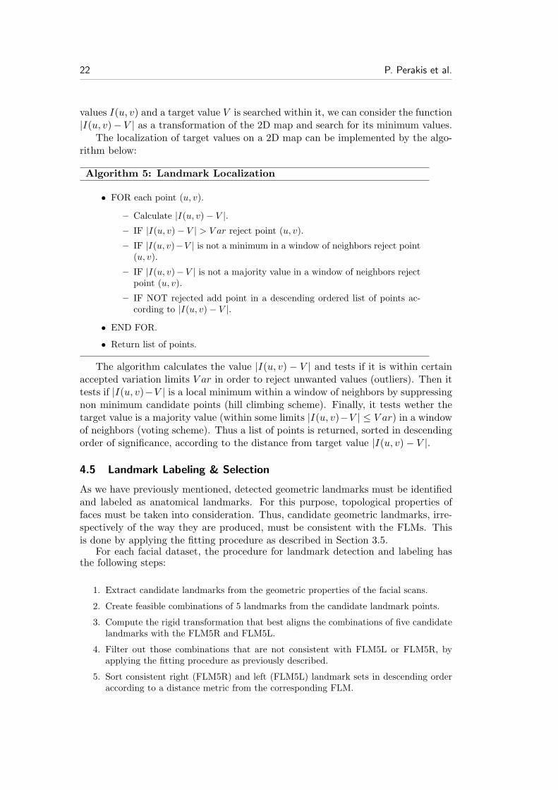
Figure 13: METHOD 1: Shape Index + Extrusion Map: Process pipeline:(a) shape index’s maxima and minima; (b) extrusion map’s candidate nose andchin tips; (c) extracted best landmark sets; (d) resulting landmarks; and (e) FacialLandmark Model (FLM) filtering.

index’s maxima that are also Extrusion’s map maxima are the candidate land-marks of the nose and chin tips (Fig. 13). To find the best solution, we used thenormalized Procrustes distance DNP (Eq. 41). This method will be referredas METHOD SIEM–NP.

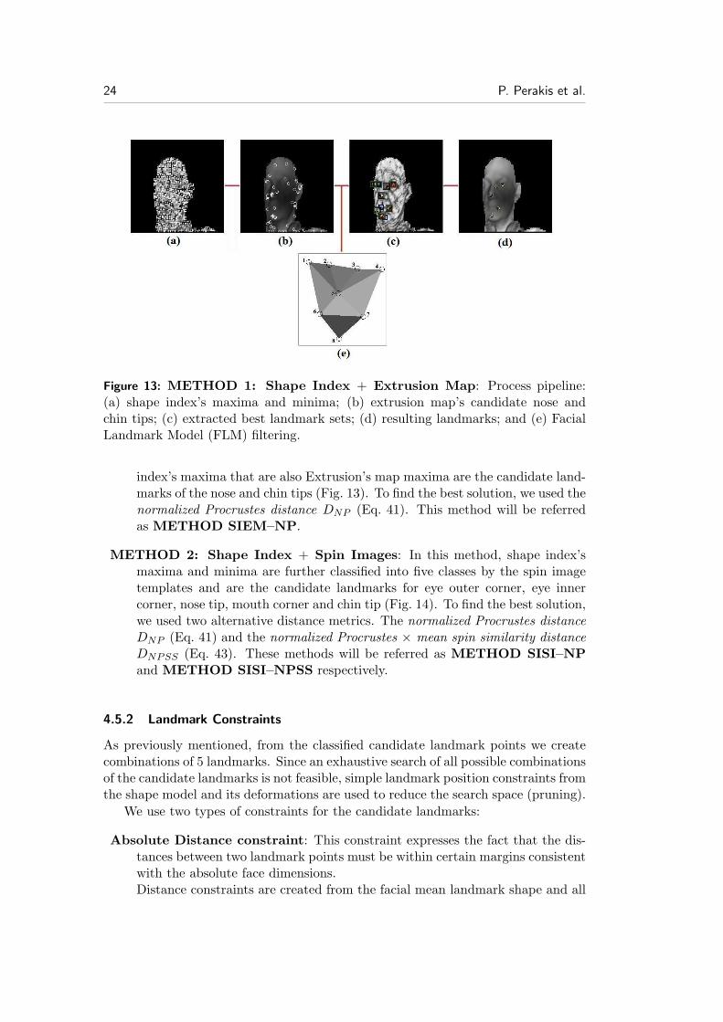
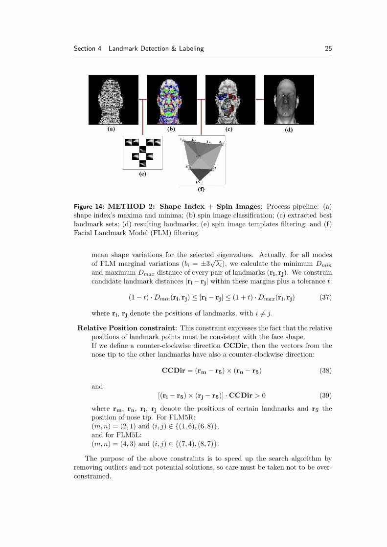
METHOD 2: Shape Index + Spin Images: In this method, shape index’smaxima and minima are further classified into five classes by the spin imagetemplates and are the candidate landmarks for eye outer corner, eye innercorner, nose tip, mouth corner and chin tip (Fig. 14). To find the best solution,we used two alternative distance metrics. The normalized Procrustes distanceDNP (Eq. 41) and the normalized Procrustes × mean spin similarity distanceDNPSS (Eq. 43). These methods will be referred as METHOD SISI–NPand METHOD SISI–NPSS respectively.

4.5.2 Landmark Constraints

As previously mentioned, from the classified candidate landmark points we createcombinations of 5 landmarks. Since an exhaustive search of all possible combinationsof the candidate landmarks is not feasible, simple landmark position constraints fromthe shape model and its deformations are used to reduce the search space (pruning).

We use two types of constraints for the candidate landmarks:

Absolute Distance constraint: This constraint expresses the fact that the dis-tances between two landmark points must be within certain margins consistentwith the absolute face dimensions.Distance constraints are created from the facial mean landmark shape and all


Figure 14: METHOD 2: Shape Index + Spin Images: Process pipeline: (a)shape index’s maxima and minima; (b) spin image classification; (c) extracted bestlandmark sets; (d) resulting landmarks; (e) spin image templates filtering; and (f)Facial Landmark Model (FLM) filtering.

mean shape variations for the selected eigenvalues. Actually, for all modesof FLM marginal variations (bi = ±3

√λi), we calculate the minimum Dmin

and maximum Dmax distance of every pair of landmarks (ri, rj). We constraincandidate landmark distances |ri− rj| within these margins plus a tolerance t:

(1− t) ·Dmin(ri, rj) ≤ |ri − rj| ≤ (1 + t) ·Dmax(ri, rj) (37)

where ri, rj denote the positions of landmarks, with i 6= j.

Relative Position constraint: This constraint expresses the fact that the relativepositions of landmark points must be consistent with the face shape.If we define a counter-clockwise direction CCDir, then the vectors from thenose tip to the other landmarks have also a counter-clockwise direction:

CCDir = (rm − r5)× (rn − r5) (38)

and[(ri − r5)× (rj − r5)] ·CCDir > 0 (39)

where rm, rn, ri, rj denote the positions of certain landmarks and r5 theposition of nose tip. For FLM5R:(m,n) = (2, 1) and (i, j) ∈ {(1, 6), (6, 8)},and for FLM5L:(m,n) = (4, 3) and (i, j) ∈ {(7, 4), (8, 7)}.

The purpose of the above constraints is to speed up the search algorithm byremoving outliers and not potential solutions, so care must be taken not to be over-constrained.


(a) (b) (c) (d)

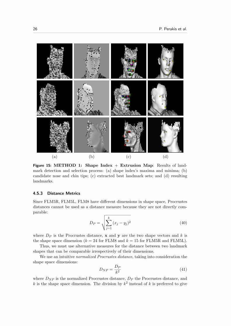
Figure 15: METHOD 1: Shape Index + Extrusion Map: Results of land-mark detection and selection process: (a) shape index’s maxima and minima; (b)candidate nose and chin tips; (c) extracted best landmark sets; and (d) resultinglandmarks.

4.5.3 Distance Metrics

Since FLM5R, FLM5L, FLM8 have different dimensions in shape space, Procrustesdistances cannot be used as a distance measure because they are not directly com-parable:

DP =

√√√√ k∑j=1

(xj − yj)2 (40)

where DP is the Procrustes distance, x and y are the two shape vectors and k isthe shape space dimension (k = 24 for FLM8 and k = 15 for FLM5R and FLM5L).

Thus, we must use alternative measures for the distance between two landmarkshapes that can be comparable irrespectively of their dimensions.

We use an intuitive normalized Procrustes distance, taking into consideration theshape space dimensions:

DNP =DP

k2(41)

where DNP is the normalized Procrustes distance, DP the Procrustes distance, andk is the shape space dimension. The division by k2 instead of k is preferred to give


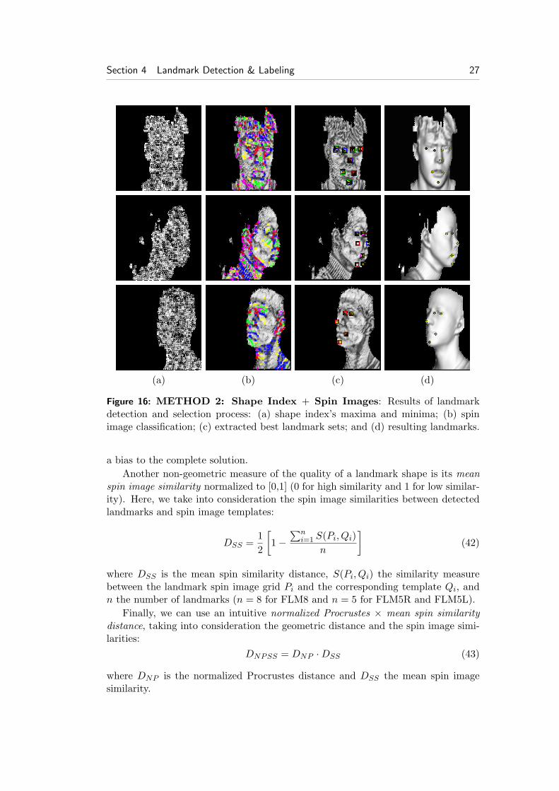
(a) (b) (c) (d)

Figure 16: METHOD 2: Shape Index + Spin Images: Results of landmarkdetection and selection process: (a) shape index’s maxima and minima; (b) spinimage classification; (c) extracted best landmark sets; and (d) resulting landmarks.

a bias to the complete solution.Another non-geometric measure of the quality of a landmark shape is its mean

spin image similarity normalized to [0,1] (0 for high similarity and 1 for low similar-ity). Here, we take into consideration the spin image similarities between detectedlandmarks and spin image templates:

DSS =12

[1−

∑ni=1 S(Pi, Qi)

n

](42)

where DSS is the mean spin similarity distance, S(Pi, Qi) the similarity measurebetween the landmark spin image grid Pi and the corresponding template Qi, andn the number of landmarks (n = 8 for FLM8 and n = 5 for FLM5R and FLM5L).

Finally, we can use an intuitive normalized Procrustes × mean spin similaritydistance, taking into consideration the geometric distance and the spin image simi-larities:

DNPSS = DNP ·DSS (43)

where DNP is the normalized Procrustes distance and DSS the mean spin imagesimilarity.


An overall measure which reflects the quality of the landmark detection processis the mean Euclidian distance between two landmark shapes in original 3D space:

DME =∑n

i=1 |xi − yi|n

(44)

where DME is the mean Euclidian distance, |xi−yi| the Euclidian distance betweenthe landmark points xi and yi of the two shapes and n the number of landmarks(n = 8 for FLM8 and n = 5 for FLM5R and FLM5L).

Another measure which reflects the quality of the registration process is themodified directed Hausdorff distance DMDH , of a face model M to a test face T ,which is defined as [Gao03]:

DMDH(M,T ) =1p

p∑mi,i=1

mintj|mi − tj | (45)

where |mi−tj | is the Euclidian distance between the face model vertices mi and thetest face vertices tj , and p the number of the face model vertices. The DMDH(M,T )expresses the mean value of the minimum Euclidian distances |mi−tj | of the verticesof the face model M , to which a test face scan T is registered.

We used the “normalized Procrustes” DNP distance metric to select the bestlandmark set solution in “Method SIEM–NP” and “Method SISI–NP”, and the“normalized Procrustes × mean spin similarity” DNPSS distance metric in “MethodSISI–NPSS”, where spin images are available. Finally, we used the “mean Euclidiandistance” DME to express the mean localization error of the landmarks and the“modified directed Hausdorff distance” DMDH to express the quality of the regis-tration process.

4.5.4 Face Registration & Pose Estimation

In a 3D face recognition system, alignment (registration) between the query andthe stored datasets is necessary in order to make the probe and the gallery datasetcomparable. Registration can be done against a common frame of reference, i.e. aReference Face Model (RFM) of known coordinates (Fig. 17). Registration of facialdatasets to a reference face model can be accomplished, by minimizing the Procrustesdistance between a set of landmark points on the facial dataset and the correspondinglandmark points on the Reference Face Model. Landmark points x on the facialdatasets have to be detected by applying one of the previously mentioned methods,and landmark points x0 on the Reference Face Model are manually annotated onceat a preprocessing stage.

Alignment of a set of face landmark points x to the RFM landmark points x0 isdone by minimizing the Procrustes distance in an iterative approach:


(a) (b) (c)

Figure 17: Reference face model (RFM) and test face superposed after alignment:(a) frontal face dataset; (b) 45◦ left side face dataset; and (c) 60◦ right side facedataset. (Gray color denotes the face model. Color range – red: near to blue: far –denotes min distances of test face vertices to model.)

Algorithm 6: Face Registration

• Calculate T to translate x so that its centroid is at the origin (0,0,0).

• Scale x shape so that its size is 1.

• Calculate T0 to translate x0 so that its centroid is at the origin (0,0,0).

• Scale x0 shape so that its size is 1.

• REPEAT

– Align x to the reference shape x0 by an optimal rotation R.

– Compute the Procrustes distance of x to the reference shape x0.

• UNTIL Convergence: |x− x0| < ε.

• Apply T−10 ·R ·T to register face data.

Thus the final transformation to register a facial dataset to an RFM is:

x′ = T0 ·R ·T · x (46)

and pose is estimated from R. Notice that scaling can be omitted when the probeand reference shapes are of the same size.

Note that the landmark set detected on the probe facial scan (complete, rightor left) determines the set of the landmarks (FLM8, FLM5R or FLM5L) used forregistration with the Reference Face Model. Fig. 17 depicts the registration of aprofile facial dataset to a RFM. Note that a left side 5 landmark set detected on thefacial scan has to be aligned with the left 5 landmark subset of the RFM, to have acorrect global registration.

As a Reference Face Model the complete Facial Landmark Model (FLM8) (Fig. 3(c))or an Annotated Face Model can be used (Fig. 18). The Annotated Face Model(AFM) [KPT∗07] is an anthropometrically correct 3D model of the human face [Far94].It is constructed only once and is used in the alignment, fitting, and metadata gener-ation for face recognition [KPT∗07, PPT∗09]. The AFM is annotated into differentareas (e.g., mouth, nose, eyes) and can have predefined landmark points. Using


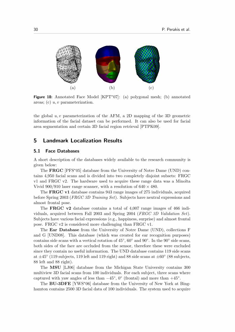
(a) (b) (c)

Figure 18: Annotated Face Model [KPT∗07]: (a) polygonal mesh; (b) annotatedareas; (c) u, v parameterization.

the global u, v parameterization of the AFM, a 2D mapping of the 3D geometricinformation of the facial dataset can be performed. It can also be used for facialarea segmentation and certain 3D facial region retrieval [PTPK09].

5 Landmark Localization Results

5.1 Face Databases

A short description of the databases widely available to the research community isgiven below:

The FRGC [PFS∗05] database from the University of Notre Dame (UND) con-tains 4,950 facial scans and is divided into two completely disjoint subsets: FRGCv1 and FRGC v2. The hardware used to acquire these range data was a MinoltaVivid 900/910 laser range scanner, with a resolution of 640× 480.

The FRGC v1 database contains 943 range images of 275 individuals, acquiredbefore Spring 2003 (FRGC 3D Training Set). Subjects have neutral expressions andalmost frontal pose.

The FRGC v2 database contains a total of 4,007 range images of 466 indi-viduals, acquired between Fall 2003 and Spring 2004 (FRGC 3D Validation Set).Subjects have various facial expressions (e.g., happiness, surprise) and almost frontalpose. FRGC v2 is considered more challenging than FRGC v1.

The Ear Database from the University of Notre Dame (UND), collections Fand G [UND08]. This database (which was created for ear recognition purposes)contains side scans with a vertical rotation of 45◦, 60◦ and 90◦. In the 90◦ side scans,both sides of the face are occluded from the sensor, therefore these were excludedsince they contain no useful information. The UND database contains 119 side scansat ±45◦ (119 subjects, 119 left and 119 right) and 88 side scans at ±60◦ (88 subjects,88 left and 88 right).

The MSU [LJ06] database from the Michigan State University contains 300multiview 3D facial scans from 100 individuals. For each subject, three scans wherecaptured with yaw angles of less than −45◦, 0◦ (frontal) and more than +45◦.

The BU-3DFE [YWS∗06] database from the University of New York at Bing-hamton contains 2500 3D facial data of 100 individuals. The system used to acquire

Section 5 Landmark Localization Results 31

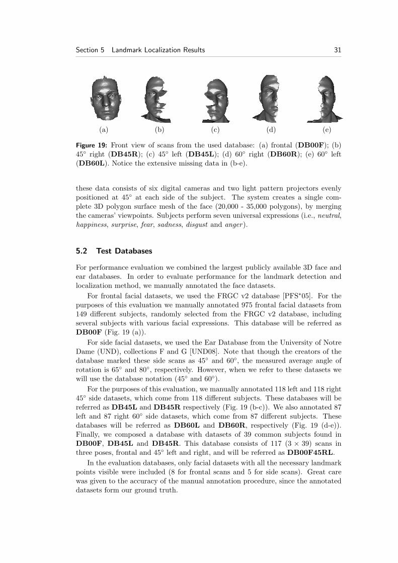
(a) (b) (c) (d) (e)

Figure 19: Front view of scans from the used database: (a) frontal (DB00F); (b)45◦ right (DB45R); (c) 45◦ left (DB45L); (d) 60◦ right (DB60R); (e) 60◦ left(DB60L). Notice the extensive missing data in (b-e).

these data consists of six digital cameras and two light pattern projectors evenlypositioned at 45◦ at each side of the subject. The system creates a single com-plete 3D polygon surface mesh of the face (20,000 - 35,000 polygons), by mergingthe cameras’ viewpoints. Subjects perform seven universal expressions (i.e., neutral,happiness, surprise, fear, sadness, disgust and anger).

5.2 Test Databases

For performance evaluation we combined the largest publicly available 3D face andear databases. In order to evaluate performance for the landmark detection andlocalization method, we manually annotated the face datasets.

For frontal facial datasets, we used the FRGC v2 database [PFS∗05]. For thepurposes of this evaluation we manually annotated 975 frontal facial datasets from149 different subjects, randomly selected from the FRGC v2 database, includingseveral subjects with various facial expressions. This database will be referred asDB00F (Fig. 19 (a)).

For side facial datasets, we used the Ear Database from the University of NotreDame (UND), collections F and G [UND08]. Note that though the creators of thedatabase marked these side scans as 45◦ and 60◦, the measured average angle ofrotation is 65◦ and 80◦, respectively. However, when we refer to these datasets wewill use the database notation (45◦ and 60◦).

For the purposes of this evaluation, we manually annotated 118 left and 118 right45◦ side datasets, which come from 118 different subjects. These databases will bereferred as DB45L and DB45R respectively (Fig. 19 (b-c)). We also annotated 87left and 87 right 60◦ side datasets, which come from 87 different subjects. Thesedatabases will be referred as DB60L and DB60R, respectively (Fig. 19 (d-e)).Finally, we composed a database with datasets of 39 common subjects found inDB00F, DB45L and DB45R. This database consists of 117 (3 × 39) scans inthree poses, frontal and 45◦ left and right, and will be referred as DB00F45RL.

In the evaluation databases, only facial datasets with all the necessary landmarkpoints visible were included (8 for frontal scans and 5 for side scans). Great carewas given to the accuracy of the manual annotation procedure, since the annotateddatasets form our ground truth.


5.3 Performance Evaluation

For the performance evaluation of the proposed landmark detection method, weconducted the following three experiments:

Experiment 1: In this experiment we used Method SIEM–NP. Thus, shape in-dex’s minima are the candidate landmarks for eye and mouth corners andshape index’s maxima that are also extrusion’s map maxima are the candi-date landmarks of the nose and chin tips. To find the best solution, we usedthe normalized Procrustes distance DNP .

Experiment 2: In this experiment we used Method SISI–NP. Thus, shape index’smaxima and minima are further classified into five classes by the spin imagetemplates and are the candidate landmarks for eye outer corner, eye innercorner, nose tip, mouth corner and chin tip. To find the best solution, we usedthe normalized Procrustes distance DNP .

Experiment 3: In this experiment we used Method SISI–NPSS. Thus, shapeindex’s maxima and minima are further classified into five classes by the spinimage templates and are the candidate landmarks for eye outer corner, eyeinner corner, nose tip, mouth corner and chin tip. To find the best solution,we used the normalized Procrustes × mean spin similarity distance DNPSS .

The performance evaluation is generally presented by calculating the followingvalues, which represent the localization accuracy of the detected landmarks:

Absolute Distance Error: It is the Euclidean distance in physical units (e.g.,mm) between the position of the detected landmark and the manually anno-tated landmark, which is considered ground truth.

Success Rate: It is the percentage of successful detections of a landmark over atested database. Successful detection is considered a detection of a landmarkwith Absolute Localization Distance Error under a certain threshold (e.g.,10 mm).

In all our experiments, the mean and standard deviation of the absolute distanceerror between the manually annotated landmarks and the automatically detectedlandmarks was calculated to represent the localization error. Also, the overall meandistance error of the 8 landmark points for the frontal datasets and of the 5 landmarkpoints for the side datasets was computed. This error is expressed with the “meanEuclidian distance” DME (Eq. 44) between the manually annotated landmarks andthe automatically detected landmarks.

Localization error analysis for the mean and standard deviation was carried outonly on results where the pose of the probe was correctly estimated, and is presentedin Tables: 2, 3, 4, 5, 6 and 7. The pose detection rate is the percentage of correct poseestimations of the probe (frontal, left profile, right profile), according to the knownpose of the probe, and which also have a mean distance error under 30.00 mm. Afalse pose estimation or a mean distance error estimation over 30.00mm is considereda pose detection failure. Also, the yaw angle is calculated and its mean value,


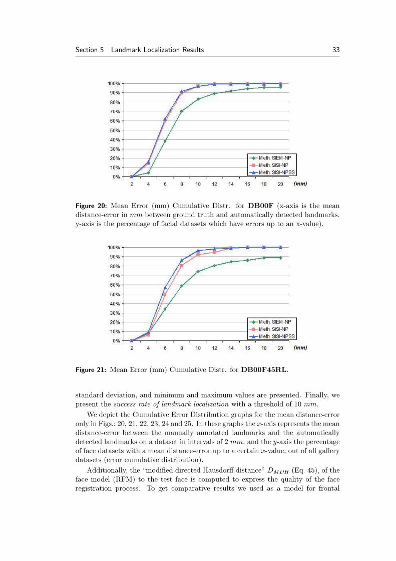
Figure 20: Mean Error (mm) Cumulative Distr. for DB00F (x-axis is the meandistance-error in mm between ground truth and automatically detected landmarks.y-axis is the percentage of facial datasets which have errors up to an x-value).

Figure 21: Mean Error (mm) Cumulative Distr. for DB00F45RL.

standard deviation, and minimum and maximum values are presented. Finally, wepresent the success rate of landmark localization with a threshold of 10 mm.

We depict the Cumulative Error Distribution graphs for the mean distance-erroronly in Figs.: 20, 21, 22, 23, 24 and 25. In these graphs the x-axis represents the meandistance-error between the manually annotated landmarks and the automaticallydetected landmarks on a dataset in intervals of 2 mm, and the y-axis the percentageof face datasets with a mean distance-error up to a certain x-value, out of all gallerydatasets (error cumulative distribution).

Additionally, the “modified directed Hausdorff distance” DMDH (Eq. 45), of theface model (RFM) to the test face is computed to express the quality of the faceregistration process. To get comparative results we used as a model for frontal


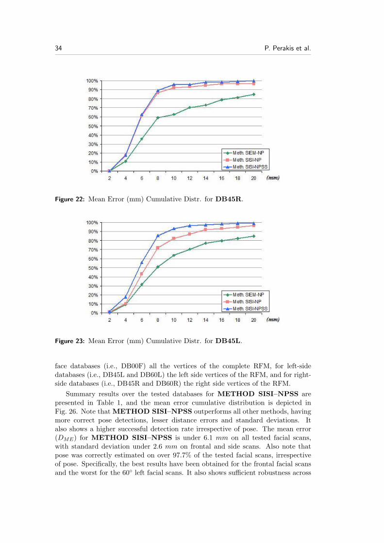
Figure 22: Mean Error (mm) Cumulative Distr. for DB45R.

Figure 23: Mean Error (mm) Cumulative Distr. for DB45L.

face databases (i.e., DB00F) all the vertices of the complete RFM, for left-sidedatabases (i.e., DB45L and DB60L) the left side vertices of the RFM, and for right-side databases (i.e., DB45R and DB60R) the right side vertices of the RFM.

Summary results over the tested databases for METHOD SISI–NPSS arepresented in Table 1, and the mean error cumulative distribution is depicted inFig. 26. Note that METHOD SISI–NPSS outperforms all other methods, havingmore correct pose detections, lesser distance errors and standard deviations. Italso shows a higher successful detection rate irrespective of pose. The mean error(DME) for METHOD SISI–NPSS is under 6.1 mm on all tested facial scans,with standard deviation under 2.6 mm on frontal and side scans. Also note thatpose was correctly estimated on over 97.7% of the tested facial scans, irrespectiveof pose. Specifically, the best results have been obtained for the frontal facial scansand the worst for the 60◦ left facial scans. It also shows sufficient robustness across


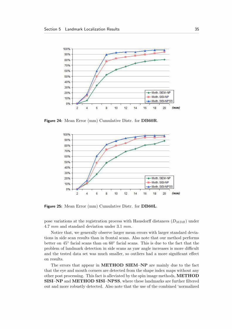
Figure 24: Mean Error (mm) Cumulative Distr. for DB60R.

Figure 25: Mean Error (mm) Cumulative Distr. for DB60L.

pose variations at the registration process with Hausdorff distances (DMDH) under4.7 mm and standard deviation under 3.1 mm.

Notice that, we generally observe larger mean errors with larger standard devia-tions in side scan results than in frontal scans. Also note that our method performsbetter on 45◦ facial scans than on 60◦ facial scans. This is due to the fact that theproblem of landmark detection in side scans as yaw angle increases is more difficultand the tested data set was much smaller, so outliers had a more significant effecton results.

The errors that appear in METHOD SIEM–NP are mainly due to the factthat the eye and mouth corners are detected from the shape index maps without anyother post processing. This fact is alleviated by the spin image methods, METHODSISI–NP and METHOD SISI–NPSS, where these landmarks are further filteredout and more robustly detected. Also note that the use of the combined ‘normalized


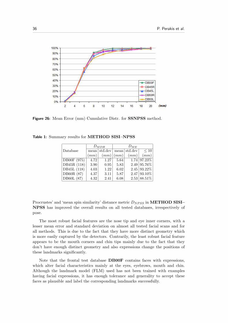
Figure 26: Mean Error (mm) Cumulative Distr. for SSNPSS method.

Table 1: Summary results for METHOD SISI–NPSS

DMDH DME

Database mean std.dev mean std.dev ≤ 10(mm) (mm) (mm) (mm) (mm)

DB00F (975) 4.72 1.27 5.64 1.74 97.23%DB45R (118) 3.90 0.95 5.83 2.49 95.76%DB45L (118) 4.03 1.22 6.02 2.45 93.22%DB60R (87) 4.37 3.11 5.87 2.47 93.10%DB60L (87) 4.32 2.41 6.08 2.53 88.51%

Procrustes’ and ‘mean spin similarity’ distance metric DNPSS in METHOD SISI–NPSS has improved the overall results on all tested databases, irrespectively ofpose.

The most robust facial features are the nose tip and eye inner corners, with alesser mean error and standard deviation on almost all tested facial scans and forall methods. This is due to the fact that they have more distinct geometry whichis more easily captured by the detectors. Contrarily, the least robust facial featureappears to be the mouth corners and chin tips mainly due to the fact that theydon’t have enough distinct geometry and also expressions change the positions ofthese landmarks significantly.

Note that the frontal test database DB00F contains faces with expressions,which alter facial characteristics mainly at the eyes, eyebrows, mouth and chin.Although the landmark model (FLM) used has not been trained with exampleshaving facial expressions, it has enough tolerance and generality to accept thesefaces as plausible and label the corresponding landmarks successfully.

Section 6 Conclusion 37

5.4 Comparative Results

For comparison of the performance of our proposed landmark detection method andother researchers’ methods, we present landmark localization errors in Tables 8 and9.

Note that each researcher uses a different facial database making direct compar-isons extremely difficult. However, the comparative results presented in Tables 8and 9 indicate that our presented METHOD SISI–NPSS outperforms previousmethods for the following reasons: (i) it is more accurate, since it gives the minimummean localization distance error for almost all landmarks, and (ii) it is more robust,since it gives the minimum standard deviation for the localization distance error.

Yu’s method [YM08] shows the minimum mean localization error for the nosetip but has a large standard deviation. Lu’s method [LJ05] shows the minimummean localization error for the mouth corners but it is not a pure 3D method,since it is assisted by 2D intensity data. Finally, Colbry’s method [Col06] seemsto behave well enough for all landmarks, comparatively close to our method, but itgives larger standard deviations. Furthermore, the database used contains a smallportion (≈ 5%) of pose variations, occlusions and expressions.

To the best of our knowledge, Lu’s method [LJ06] is the only one that presentedlocalization errors on mixed frontal and profile facial datasets. Although it showssmall mean localization errors for the mouth corners, it has a large standard devi-ation. On the other hand, the tested MSU database consists of a larger number offacial datasets.

Notice that for our methods, the same parameters were used in all cases (acrossfrontal, semi-profile and profile scans). If the proposed methods are applied todatabases restricted only to frontal scans or only to profile scans, the parameterscan be fine-tuned to achieve higher performance.

5.5 Computational Efficiency

For the evaluation of the proposed method’s computational efficiency, a typical mod-ern PC was used: Intel Core 2 Duo 2.2GHz, 2GB RAM, NVIDIA GeForce 8600GTS.Using this PC, 9 seconds on average are required for each facial scan to locate thefacial landmarks. The procedures of determining the optimal rotation for the align-ment of the landmark shapes to the FLMs require at most 8 iterations to converge.The registration step (that takes 8 iterations to converge) requires less than 0.1 sec,depending on dataset size. The computational efficiency of the proposed landmarkdetection and registration method makes it suitable for real-world applications.

6 Conclusion

We have presented an automatic 3D facial landmark detection method that offerspose invariance and robustness to large missing facial areas, with respect to ex-treme pose variations. The proposed approach introduced new methods for 3Dlandmark localization by exploiting the 3D geometry-based information of faces andthe modeling ability of trained landmark models. It has been evaluated using the


most challenging 3D facial databases available that include pose variations up to80◦ along the vertical axis. All steps of the method (landmark detection and poseestimation for registration) work robustly, even if half of the face is missing.

Future work will be directed towards increasing the robustness and accuracy ofthe landmark detector. This could be accomplished in two ways: firstly by increasingthe examples datasets for creating the facial landmark model, including expressionvariations, and secondly by increasing the landmark set, including the nostrils base.

REFERENCES 39

References

[CCRA∗05] Conde C., Cipolla R., Rodrıgez-Aragon L. J., Serrano A.,Cabello E.: 3D facial feature location with spin images. In Proc.IAPR Conference on Machine Vision Applications (Tsukuba ScienceCity, Japan, May 16 – 18 2005), pp. 418–421.

[Col06] Colbry D.: Human Face Verification by Robust 3D Surface Alignment.PhD thesis, Michigan State University, 2006.

[CSJ05] Colbry D., Stockman G., Jain A.: Detection of anchor points for3D face verification. In Proc. IEEE Computer Society Conference onComputer Vision and Pattern Recognition (San Diego, CA, Jun. 20-252005), p. 118.

[CT01] Cootes T., Taylor C.: Statistical Models of Appearance for Com-puter Vision. Tech. rep., University of Manchester, Oct. 2001.

[CTCG95] Cootes T., Taylor C., Cooper D., Graham J.: Active shapemodels - their training and application. Computer Vision and ImageUnderstanding 61, 1 (Jan. 1995), 38–59.

[CTKP05] Cootes T., Taylor C., Kang H., Petrovic V.: Handbook of FaceRecognition. Springer, 2005, ch. Modeling Facial Shape and Appearance,pp. 39–63.

[Dib08] Dibeklioglu H.: Part-Based 3D Face Recognition under Pose andExpression Variations. Master’s thesis, Bogazici University, 2008.

[DJ97] Dorai C., Jain A. K.: COSMOS - a representation scheme for 3Dfree-form objects. IEEE Transactions on Pattern Analysis and MachineIntelligence 19, 10 (Oct. 1997), 1115–1130.

[DM98] Dryden I., Mardia K.: Statistical Shape Analysis. Wiley, 1998.

[DSA08] Dibeklioglu H., Salah A., Akarun L.: 3D facial landmarking un-der expression, pose, and occlusion variations. In Proc. 2nd IEEE Inter-national Conference on Biometrics: Theory, Applications and Systems(Arlington, VA, Sep. 20 - Oct. 1 2008), pp. 1–6.

[Far94] Farkas L.: Anthropometry of the head and face, 2nd ed. Raven Press,1994.

[FBF08a] Faltemier T., Bowyer K., Flynn P.: A region ensemble for 3-D face recognition. IEEE Transactions on Information Forensics andSecurity 3, 1 (Mar. 2008), 62–73.

[FBF08b] Faltemier T., Bowyer K., Flynn P.: Rotated profile signaturesfor robust 3D feature detection. In Proc. 8th IEEE International Con-ference on Automatic Face and Gesture Recognition (Amsterdam, TheNetherlands, Sep. 17-19 2008), pp. 1–7.

40 REFERENCES

[Gao03] Gao Y.: Efficiently comparing face images using a modified Haus-dorff distance. In Proc. IEEE Conference on Vision, Image and SignalProcessing (Dec. 2003), pp. 346–350.

[HS88] Harris C., Stephens M.: A combined corner and edge detector. InProc. 4th Alvey Vision Conference (1988), pp. 147–151.

[Joh97] Johnson A. E.: Spin Images: A Representation for 3-D SurfaceMatching. PhD thesis, Robotics Institute, Carnegie Mellon University,Pittsburgh, PA, Aug. 1997.

[KPT∗07] Kakadiaris I., Passalis G., Toderici G., Murtuza M., Lu Y.,Karampatziakis N., Theoharis T.: Three-dimensional face recog-nition in the presence of facial expressions: An annotated deformablemodel approach. IEEE Transactions on Pattern Analysis and MachineIntelligence 29, 4 (Apr. 2007), 640–649.

[KvD92] Koenderink J., van Doorn A.: Surface shape and curvature scales.Image and Vision Computing 10 (Oct. 1992), 557–565.

[LJ05] Lu X., Jain A.: Multimodal Facial Feature Extraction for Automatic3D Face Recognition. Tech. Rep. MSU-CSE-05-22, Michigan State Uni-versity, Oct. 2005.

[LJ06] Lu X., Jain A.: Automatic feature extraction for multiview 3D facerecognition. In Proc. 7th International Conference on Automatic Faceand Gesture Recognition (Southampton, UK, Apr. 10-12 2006), pp. 585–590.

[LJC06] Lu X., Jain A., Colbry D.: Matching 2.5D face scans to 3D models.IEEE Transactions on Pattern Analysis and Machine Intelligence 28, 1(2006), 31–43.

[LSCH06] Lin T., Shih W., Chen W., Ho W.: 3D face authentication bymutual coupled 3D and 2D feature extraction. In Proc. 44th ACMSoutheast Regional Conference (Melbourne, FL, Mar. 10 – 12 2006),pp. 423–427.

[MBO07] Mian A., Bennamoun M., Owens R.: An efficient multimodal 2D-3D hybrid approach to automatic face recognition. IEEE Transactionson Pattern Analysis and Machine Intelligence 29, 11 (Nov. 2007), 1927–1943.

[NC09] Nair P., Cavallaro A.: 3-D face detection, landmark localization,and registration using a point distribution model. IEEE Transactionson Multimedia 11, 4 (June 2009), 611–623.

[PFS∗05] Phillips P., Flynn P., Scruggs T., Bowyer K., Chang J., Hoff-man K., Marques J., Min J., Worek W.: Overview of the FaceRecognition Grand Challenge. In Proc. IEEE Conference on ComputerVision and Pattern Recognition (San Diego, CA, 2005), pp. 947–954.

REFERENCES 41

[PPT∗09] Perakis P., Passalis G., Theoharis T., Toderici G., Kakadi-aris I.: Partial matching of interpose 3D facial data for face recog-nition. In Proc. 3rd IEEE International Conference on Biometrics:Theory, Applications and Systems (Arlington, VA, Sep. 28-30 2009),pp. 439–446.

[PTPK09] Perakis P., Theoharis T., Passalis G., Kakadiaris I.: Auto-matic 3D facial region retrieval from multi-pose facial datasets. InProc. Eurographics Workshop on 3D Object Retrieval (Munich, Ger-many, Mar. 30 - Apr. 3 2009), pp. 37–44.

[RHP08] Romero-Huertas M., Pears N.: 3D facial landmark localization bymatching simple descriptors. In Proc. 2nd IEEE International Confer-ence on Biometrics: Theory, Applications and Systems (Arlington, VA,Sep. 20 - Oct. 1 2008).

[SG02] Stegman M., Gomez D.: A Brief Introduction to Statistical ShapeAnalysis. Tech. rep., Technical University of Denmark, Mar. 2002.

[SQBS07] Segundo M., Queirolo C., Bellon O., Silva L.: Automatic 3Dfacial segmentation and landmark detection. In Proc. 14th InternationalConference on Image Analysis and Processing (Modena, Italy, Sep. 10-14 2007), pp. 431–436.

[TK06] Theodoridis S., Koutroumbas K.: Pattern Recognition, 3rd ed.Academic Press, 2006.

[UND08] UND: University of Notre Dame biometrics database.http://www.nd.edu/∼cvrl/UNDBiometricsDatabase.html, 2008.

[WLY07] Wei X., Longo P., Yin L.: LNCS, Advances in Biometrics. Springer,2007, ch. Automatic Facial Pose Determination of 3D Range Data forFace Model and Expression Identification, pp. 144–153.

[XTWQ06] Xu C., Tan T., Wang Y., Quan L.: Combining local features forrobust nose location in 3D facial data. Pattern Recognition Letters 27,13 (2006), 62–73.

[YM08] Yu T., Moon Y.: A novel genetic algorithm for 3D facial landmarklocalization. In Proc. 2nd IEEE International Conference on Biometrics:Theory, Applications and Systems (Arlington, VA, Sep. 20 - Oct. 12008).

[YWS∗06] Yin L., Wei X., Sun Y., Wang J., Rosato M.: A 3D facial ex-pression database for facial behavior research. In Proc. 7th InternationalConference on Automatic Face and Gesture Recognition (Southampton,UK, Apr. 10-12 2006), pp. 211–216.


A Results Tables

Section A Results Tables 43

Table 2: Results for DB00F

Experiment 1: METHOD SIEM–NPCorrect Pose Detection 947 / 975 97.13%Yaw Estimation −0.94◦ ± 5.58◦ [−14.57◦ ∼ +19.53◦]Localization Error mean (mm) std.dev. (mm) ≤ 10 mmRight Eye Outer Corner 6.92 4.47 77.64%Right Eye Inner Corner 6.18 3.71 86.26%Left Eye Inner Corner 6.85 3.63 83.69%Left Eye Outer Corner 7.18 4.84 75.90%Nose Tip 6.32 4.12 86.87%Mouth Right Corner 7.42 5.60 71.18%Mouth Left Corner 7.84 5.22 68.72%Chin Tip 10.26 6.59 58.67%Mean Distance Error 7.37 3.20 83.18%

Experiment 2: METHOD SISI–NPCorrect Pose Detection 970 / 975 99.49%Yaw Estimation −0.63◦ ± 5.02◦ [−13.95◦ ∼ +16.47◦]Localization Error mean (mm) std.dev. (mm) ≤ 10 mmRight Eye Outer Corner 5.87 3.52 86.56%Right Eye Inner Corner 5.19 2.54 94.56%Left Eye Inner Corner 5.59 2.63 94.36%Left Eye Outer Corner 5.81 3.71 87.79%Nose Tip 5.28 2.40 96.10%Mouth Right Corner 5.71 4.30 83.69%Mouth Left Corner 6.47 4.14 82.15%Chin Tip 6.30 4.36 88.21%Mean Distance Error 5.78 1.78 97.23%

Experiment 3: METHOD SISI–NPSSCorrect Pose Detection 970 / 975 99.49%Yaw Estimation −0.63◦ ± 5.02◦ [−13.95◦ ∼ +16.47◦]Localization Error mean (mm) std.dev. (mm) ≤ 10 mmRight Eye Outer Corner 5.82 3.43 87.18%Right Eye Inner Corner 5.10 2.53 94.87%Left Eye Inner Corner 5.52 2.56 94.56%Left Eye Outer Corner 5.70 3.52 88.10%Nose Tip 4.88 2.42 96.72%Mouth Right Corner 5.64 4.26 84.62%Mouth Left Corner 6.42 4.17 82.15%Chin Tip 6.03 4.27 89.54%Mean Distance Error 5.64 1.74 97.23%


Table 3: Results for DB00F45RL

Experiment 1: METHOD SIEM–NPCorrect Pose Detection 105 / 117 89.74%Yaw Estimation −1.32◦ ± 36.50◦ [−66.09◦ ∼ +79.81◦]Localization Error mean (mm) std.dev. (mm) ≤ 10 mmRight Eye Outer Corner 7.17 3.96 68.55%Right Eye Inner Corner 6.74 3.65 76.03%Left Eye Inner Corner 7.60 3.69 72.29%Left Eye Outer Corner 7.91 4.71 64.81%Nose Tip 6.61 4.92 76.92%Mouth Right Corner 6.17 5.22 74.79%Mouth Left Corner 7.29 5.64 68.55%Chin Tip 8.85 6.02 63.25%Mean Distance Error 7.49 3.32 74.36%

Experiment 2: METHOD SISI–NPCorrect Pose Detection 117 / 117 100.00%Yaw Estimation −1.45◦ ± 37.05◦ [−67.39◦ ∼ +60.58◦]Localization Error mean (mm) std.dev. (mm) ≤ 10 mmRight Eye Outer Corner 6.91 3.94 71.79%Right Eye Inner Corner 5.87 3.17 89.74%Left Eye Inner Corner 6.78 2.97 87.18%Left Eye Outer Corner 6.82 3.89 78.21%Nose Tip 5.62 3.70 87.18%Mouth Right Corner 6.13 4.56 84.62%Mouth Left Corner 7.05 4.72 78.21%Chin Tip 6.79 4.50 84.62%Mean Distance Error 6.55 2.26 92.31%

Experiment 3: METHOD SISI–NPSSCorrect Pose Detection 117 / 117 100.00%Yaw Estimation −1.45◦ ± 37.05◦ [−67.39◦ ∼ +60.58◦]Localization Error mean (mm) std.dev. (mm) ≤ 10 mmRight Eye Outer Corner 6.49 3.93 76.92%Right Eye Inner Corner 5.91 3.02 92.31%Left Eye Inner Corner 6.90 2.85 85.90%Left Eye Outer Corner 6.40 3.74 79.49%Nose Tip 4.30 2.93 94.02%Mouth Right Corner 5.70 4.10 87.18%Mouth Left Corner 6.20 4.30 83.33%Chin Tip 6.40 4.17 87.18%Mean Distance Error 5.96 1.92 96.58%


Table 4: Results for DB45R

Experiment 1: METHOD SIEM–NPCorrect Pose Detection 100 / 118 84.75%Yaw Estimation +44.39◦ ± 8.83◦ [+18.09◦ ∼ +79.81◦]Localization Error mean (mm) std.dev. (mm) ≤ 10 mmRight Eye Outer Corner 7.60 4.73 61.86%Right Eye Inner Corner 6.46 3.70 68.64%Nose Tip 7.69 6.69 66.95%Mouth Right Corner 7.12 6.60 62.71%Chin Tip 10.23 7.79 55.08%Mean Distance Error 7.82 4.21 62.71%

Experiment 2: METHOD SISI–NPCorrect Pose Detection 115 / 118 97.46%Yaw Estimation +43.25◦ ± 8.13◦ [+20.07◦ ∼ +71.42◦]Localization Error mean (mm) std.dev. (mm) ≤ 10 mmRight Eye Outer Corner 6.31 3.90 77.12%Right Eye Inner Corner 6.17 3.43 84.75%Nose Tip 5.50 4.39 87.29%Mouth Right Corner 5.70 4.80 80.51%Chin Tip 6.00 4.75 87.29%Mean Distance Error 5.93 2.51 92.37%

Experiment 3: METHOD SISI–NPSSCorrect Pose Detection 118 / 118 100.00%Yaw Estimation +43.35◦ ± 8.26◦ [+20.07◦ ∼ +71.42◦]Localization Error mean (mm) std.dev. (mm) ≤ 10 mmRight Eye Outer Corner 6.62 3.73 80.51%Right Eye Inner Corner 6.03 3.29 88.14%Nose Tip 4.39 3.47 94.92%Mouth Right Corner 5.96 4.98 81.36%Chin Tip 6.17 5.21 92.37%Mean Distance Error 5.83 2.49 95.76%


Table 5: Results for DB45L

Experiment 1: METHOD SIEM–NPCorrect Pose Detection 105 / 118 88.98%Yaw Estimation −47.19◦ ± 9.19◦ [−84.14◦ ∼ −19.43◦]Localization Error mean (mm) std.dev. (mm) ≤ 10 mmLeft Eye Outer Corner 8.41 5.62 60.17%Left Eye Inner Corner 8.09 4.53 63.56%Nose Tip 8.21 7.89 66.95%Mouth Left Corner 9.50 7.48 56.78%Chin Tip 10.37 7.36 57.63%Mean Error 8.92 5.17 63.56%

Experiment 2: METHOD SISI–NPCorrect Pose Detection 115 / 118 97.46%Yaw Estimation −45.71◦ ± 8.58◦ [−68.17◦ ∼ −13.83◦]Localization Error mean (mm) std.dev. (mm) ≤ 10 mmLeft Eye Outer Corner 7.00 5.08 77.12%Left Eye Inner Corner 7.02 3.93 81.36%Nose Tip 6.82 5.00 78.81%Mouth Left Corner 8.17 5.89 67.80%Chin Tip 7.18 5.63 78.81%Mean Distance Error 7.24 3.48 82.20%

Experiment 3: METHOD SISI–NPSSCorrect Pose Detection 117 / 118 99.15%Yaw Estimation −45.43◦ ± 8.76◦ [−68.17◦ ∼ −13.83◦]Localization Error mean (mm) std.dev. (mm) ≤ 10 mmLeft Eye Outer Corner 6.39 4.21 77.12%Left Eye Inner Corner 6.61 3.04 86.44%Nose Tip 4.02 2.70 95.76%Mouth Left Corner 6.79 5.28 77.12%Chin Tip 6.29 4.62 85.59%Mean Distance Error 6.02 2.45 93.22%


Table 6: Results for DB60R

Experiment 1: METHOD SIEM–NPCorrect Pose Detection 72 / 87 82.76%Yaw Estimation +58.11◦ ± 6.70◦ [+32.10◦ ∼ +74.89◦]Localization Error mean (mm) std.dev. (mm) ≤ 10 mmRight Eye Outer Corner 7.30 5.34 63.22%Right Eye Inner Corner 6.81 4.83 70.11%Nose Tip 7.51 5.05 70.11%Mouth Right Corner 8.02 7.48 55.17%Chin Tip 11.55 8.87 43.68%Mean Distance Error 8.24 4.43 62.07%

Experiment 2: METHOD SISI–NPCorrect Pose Detection 82 / 87 94.25%Yaw Estimation +57.00◦ ± 7.19◦ [+31.22◦ ∼ +74.60◦]Localization Error mean (mm) std.dev. (mm) ≤ 10 mmRight Eye Outer Corner 7.11 5.26 74,71%Right Eye Inner Corner 5.90 4.33 83.91%Nose Tip 5.56 4.45 85.06%Mouth Right Corner 7.01 5.87 71.26%Chin Tip 8.04 6.07 71.26%Mean Distance Error 6.72 3.55 82.76%

Experiment 3: METHOD SISI–NPSSCorrect Pose Detection 85 / 87 97.70%Yaw Estimation +56.97◦ ± 7.38◦ [+31.22◦ ∼ +74.60◦]Localization Error mean (mm) std.dev. (mm) ≤ 10 mmRight Eye Outer Corner 6.88 4.34 77.01%Right Eye Inner Corner 5.81 3.39 86.21%Nose Tip 3.98 3.20 95.40%Mouth Right Corner 6.29 5.08 79.31%Chin Tip 6.38 4.85 85.06%Mean Distance Error 5.87 2.47 93.10%


Table 7: Results for DB60L

Experiment 1: METHOD SIEM–NPCorrect Pose Detection 78 / 87 89.66%Yaw Estimation −60.57◦ ± 8.71◦ [−87.87◦ ∼ −38.61◦]Localization Error mean (mm) std.dev. (mm) ≤ 10 mmLeft Eye Outer Corner 7.41 5.30 67.82%Left Eye Inner Corner 8.11 4.60 64.37%Nose Tip 7.25 6.43 71.26%Mouth Left Corner 10.66 7.46 49.43%Chin Tip 10.76 7.64 54.02%Mean Distance Error 8.84 4.52 58.62%

Experiment 2: METHOD SISI–NPCorrect Pose Detection 83 / 87 95.40%Yaw Estimation −57.63◦ ± 7.46◦ [−74.41◦ ∼ −32.49◦]Localization Error mean (mm) std.dev. (mm) ≤ 10 mmLeft Eye Outer Corner 5.56 3.73 83.91%Left Eye Inner Corner 6.66 3.24 79.31%Nose Tip 5.49 4.63 83.91%Mouth Left Corner 8.36 6.19 66.67%Chin Tip 8.20 6.60 72.41%Mean Distance Error 6.85 3.27 79.31%

Experiment 3: METHOD SISI–NPSSCorrect Pose Detection 85 / 87 97.70%Yaw Estimation −57.46◦ ± 7.45◦ [−74.41◦ ∼ −32.49◦]Localization Error mean (mm) std.dev. (mm) ≤ 10 mmLeft Eye Outer Corner 5.66 3.45 87.36%Left Eye Inner Corner 6.54 3.15 85.06%Nose Tip 3.67 1.98 95.40%Mouth Left Corner 7.78 5.93 73.56%Chin Tip 6.77 6.02 81.61%Mean Distance Error 6.08 2.53 88.51%


Table 8: Comparison of landmark localization error of different approaches onalmost-frontal complete facial datasets

Mean Localization Error (mm)Method Test DB (scans) REIC LEIC REOC LEOC NT CT MRC MLC[YM08] (GA model) FRGC v1 (200) 4.74 5.59 - - 2.18 - - -[NC09] (w/o PDM) BU-3DFE (2350) 25.01 26.68 31.84 34.39 14.59 - - -

(w PDM) 12.11 11.89 20.46 19.38 8.83 - - -[LJ06] (3D) FRGC v1 (953) 8.30 8.20 9.50 10.30 8.30 - 6.00 6.20[LJ05] (3D+2D) FRGC v1 (946) 6.00 5.70 7.10 7.90 5.00 - 3.60 3.60[Col06] (w/o CFDM) FRGC v1 (953) 5.50 6.30 - - 4.10 11.00 6.90 6.70

(w CFDM) + propr. (160) 5.60 6.00 - - 4.00 11.70 5.40 5.40[PTPK09] (EG-3DOR) FRGC v2 (975) 7.02 7.46 8.13 9.21 5.23 6.71 8.30 9.83Perakis et al. (current) (SIEM–NP) FRGC v2 (975) 6.18 6.85 6.92 7.18 6.32 10.26 7.42 7.84

(SISI–NP) 5.19 5.59 5.87 5.81 5.28 6.30 5.71 6.47(SISI–NPSS) 5.10 5.52 5.82 5.70 4.88 6.03 5.64 6.42

Std. Dev. of Localization Error (mm)Method Test DB (scans) REIC LEIC REOC LEOC NT CT MRC MLC[YM08] (GA model) FRGC v1 (200) 9.76 16.08 - - 6.83 - - -[NC09] (w/o PDM) BU-3DFE (2350) - - - - - - - -

(w PDM) - - - - - - - -[LJ06] (3D) FRGC v1 (953) 17.20 17.20 17.10 18.10 19.40 - 16.90 17.90[LJ05] (3D+2D) FRGC v1 (946) 3.30 3.00 5.90 5.10 2.40 - 3.30 2.90[Col06] (w/o CFDM) FRGC v1 (953) 4.90 5.00 - - 5.10 7.60 8.60 9.30

(w CFDM) + propr. (160) 4.80 4.70 - - 5.40 7.30 6.80 6.70[PTPK09] (EG-3DOR) FRGC v2 (975) 3.18 3.07 3.79 4.25 3.28 4.32 4.53 4.47Perakis et al. (current) (SIEM–NP) FRGC v2 (975) 3.71 3.63 4.47 4.84 4.12 6.59 5.60 5.22

(SISI–NP) 2.54 2.63 3.52 3.71 2.40 4.36 4.30 4.14(SISI–NPSS) 2.53 2.56 3.43 3.52 2.42 4.27 4.26 4.17

Landmarks:REIC & LEIC: Right and Left Eye Inner CornersREOC & LEOC: Right and Left Eye Outer CornersNT & CT: Nose and Chin TipsMRC & MLC: Mouth Right and Left Corners

Table 9: Comparison of landmark localization error of different approaches on mixed(frontal and profile) facial datasets

Mean Localization Error (mm)Method Test DB (scans) REIC LEIC REOC LEOC NT CT MRC MLC[LJ06] (3D) MSU (300) 9.00 7.10 13.60 13.30 6.40 - 6.70 5.20Perakis et al. (current) (SIEM–NP) FRGC v2 6.74 7.60 7.17 7.91 6.61 8.85 6.17 7.29

(SISI–NP) + Ear (UND) 5.87 6.78 6.91 6.82 5.62 6.79 6.13 7.05(SISI–NPSS) (117) 5.91 6.90 6.49 6.40 4.30 6.40 5.70 6.20

Std. Dev. of Localization Error (mm)Method Test DB (scans) REIC LEIC REOC LEOC NT CT MRC MLC[LJ06] (3D) MSU (300) 13.10 9.20 11.90 10.10 13.40 - 12.90 9.00Perakis et al. (current) (SIEM–NP) FRGC v2 3.65 3.69 3.96 4.71 4.92 6.02 5.22 5.64

(SISI–NP) + Ear (UND) 3.17 2.97 3.94 3.89 3.70 4.50 4.56 4.72(SISI–NPSS) (117) 3.02 2.85 3.93 3.74 2.93 4.17 4.10 4.30

Landmarks:REIC & LEIC: Right and Left Eye Inner CornersREOC & LEOC: Right and Left Eye Outer CornersNT & CT: Nose and Chin TipsMRC & MLC: Mouth Right and Left Corners

3d facial landmark detection & face...

Documents