3d printed heat exchangers an experimental study...1.3 heat exchanger a heat exchanger is a thermal...
TRANSCRIPT
3D Printed Heat Exchangers
An Experimental Study
by
Gokul Chandrasekaran
A Thesis Presented in Partial Fulfillment of the Requirements for the Degree
Master of Science
Approved April 2018 by the Graduate Supervisory Committee:
Patrick Phelan, Chair Konrad Rykaczewski
Karl Schultz
ARIZONA STATE UNIVERSITY
May 2018
i
ABSTRACT
As additive manufacturing grows as a cost-effective method of manufacturing,
lighter, stronger and more efficient designs emerge. Heat exchangers are one of the most
critical thermal devices in the thermal industry. Additive manufacturing brings us a design
freedom no other manufacturing technology offers. Advancements in 3D printing lets us
reimagine and optimize the performance of the heat exchangers with an incredible design
flexibility previously unexplored due to manufacturing constraints.
In this research, the additive manufacturing technology and the heat exchanger
design are explored to find a unique solution to improve the efficiency of heat exchangers.
This includes creating a Triply Periodic Minimal Surface (TPMS) geometry, Schwarz-D in
this case, using Mathematica with a flexibility to control the cell size of the models
generated. This model is then encased in a closed cubical surface with manifolds for fluid
inlets and outlets before 3D printed using the polymer nylon for thermal evaluation.
In the extent of this study, the heat exchanger developed is experimentally
evaluated. The data obtained are used to derive a relationship between the heat transfer
effectiveness and the Number of Transfer Units (NTU).The pressure loss across a fluid
channel of the Schwarz D geometry is also studied.
The data presented in this study are part of initial experimental evaluation of 3D
printed TPMS heat exchangers.Among heat exchangers with similar performance, the
Schwarz D geometry is 32% smaller compared to a shell-and-tube heat exchanger.

ii
ACKNOWLEDGMENTS
This study was accomplished under the mentorship of Prof Pat Phelan and with immense
help from the Additive Manufacturing Group. I’m grateful to work under his mentorship. I
also would like to thank my friends and family for supporting me throughout my Master’s
Program.

iii
TABLE OF CONTENTS
Page
LIST OF TABLES ..................................................................................................................................... v
LIST OF FIGURES ................................................................................................................................. vi
NOMENCLATURE .............................................................................................................................. viii
CHAPTER
1 INTRODUCTION .............................................................................................................. 1
1.1 Triply Periodic Minimal Surface .................................................................................... 1
1.2 Additive Manufacturing .................................................................................................. 3
1.3 Heat Exchanger ................................................................................................................ 5
2 APPROACH .......................................................................................................................... 7
2.1 Heat Exchanger Design .................................................................................................. 7
2.1.1 Fabrication .................................................................................................................... 13
2.2 Experimental Setup ........................................................................................................ 15
2.1.1 Data Aquisition ............................................................................................................ 21
2.3 Errors and Uncertainities .............................................................................................. 23
2.4 Procedure for Analysis .................................................................................................. 24
3 RESULTS ............................................................................................................................. 25
3.1 Temperature .................................................................................................................... 25
3.2 Heat Transfer Rate ......................................................................................................... 30
3.3 휀 V NTU Relationship .................................................................................................. 31
3.4 Pressure Drop ................................................................................................................. 32
3.5 Comparison to Conventional Heat Exchangers ..................................................... 33

iv
CHAPTER Page
3.6 Estimating Overall Heat Transfer Coefficient, U .................................................... 36
3.7 Discussions ..................................................................................................................... 37
4 CONCLUSION .................................................................................................................. 38
5 FUTURE WORK ............................................................................................................... 39
REFERENCES ....................................................................................................................................... 40
APPENDIX
A MATHEMATICA CODE ..................................................................................................... 42
B STEADY STATE TEMPERATURE DATA ................................................................... 44

v
LIST OF TABLES
Table Page
1. Thermal Properties of Nylon -12 (PA 2200) ................................................................... 15
2. Summary of Uncertainties in the Experiment .................................................................. 26
3. Average Steady State Temperature Data .......................................................................... 25
4. Different Heat Transfer Rates Calculated from the Data ............................................. 30
5. Pressure Measurements ....................................................................................................... 32
6. Friction Factors for Schwarz D Geometry and Shell-and-tube ......................................... 35
vi
LIST OF FIGURES
Figure Page
1. Plateau’s Memory by A.van der Net ..................................................................................... 1
2. Schwarz D, Schwarz G, Schwarz P geometries ................................................................ 2
3. A Representation of Schwarz D Geometry using Mathematica ................................... 3
4. EOS P110 SLS printer ........................................................................................................... 5
5. Dynamic Window in Mathematica to Manipulate the Schawarz D Geometry .......... 8
6. Discretized Graphic of the Schwarz D Geometry ........................................................... 9
7. Geometry Region Meshed .................................................................................................. 10
8. Heat Exchanger in STL Format Generated using Mathematica ................................. 11
9. Heat Exchanger with Fefined Fluid Channels ................................................................ 12
10. X-Ray View of the Heat Exchanger ................................................................................... 12
11. Visualizing the Two Flow Paths (Red and Blue) Inside a Schwarz D Core ............... 13
12. Fabricated Schwarz D Heat Exchanger .......................................................................... 14
13. Photograph of the Experimental Setup ............................................................................. 16
14. Schematic of the Experimental Setup ................................................................................ 16
15. Thermocouple Arangement in Hot Fluid Side ................................................................ 17
16. Manometer Arrangement ..................................................................................................... 18
17. Hot and Cold Fluid Reservoirs along with the Ice Chest on the Cold Side ............... 19
18. Side View of the Heat Exchanger Mounted in the Setup ............................................. 20
19. Top View of the Heat Exchanger Mounted in the Setup ............................................. 21
20. Thermostat used for Calibrating the Thermocouples .................................................... 22
21. Temperature Profile of Hot Inlet and Outlet Temperatures for Trial 2 .................... 27
22. Temperature Profile of Cold Inlet and Outlet Temperatures for Trial 2 ................... 28

vii
Figure Page
23. Transient State Response in Hot Side for Trial 2 ............................................................ 29
24. Transient State Response in Cold Side for Trial 2 ........................................................... 29
25. 휀 v NTU Data for Different Capacity Ratios ................................................................. 31
26. Pressure Loss v Flow Rate in Schwarz D Heat Exchanger .......................................... 33
27. Friction Factor v Reynolds Number .................................................................................... 36
viii
NOMENCLATURE
𝑇ℎ𝑖 Hot Inlet Temperature [oC]
𝑇ℎ𝑜 Hot Outlet Temperature [oC]
𝑇𝑐𝑖 Cold Inlet Temperature [oC]
𝑇𝑐𝑜 Cold Outlet Temperature [oC]
𝐿𝑒 Entrance Length [m]
𝑅𝑒 Reynolds Number [-]
𝑑 Pipe Diameter [m]
�� Fluid Flow Rate [m3s-1]
�� Heat Transfer [W]
𝐶𝑝 Specific Heat of Water [J kg-1K-1]
𝜌 Density of Water [kg m-3]
𝛿 Incremental Change [-]
𝑈 Overall Heat Transfer Coefficient [W m-2 K-1]
𝐴 Area [m2]
∆𝑇𝐿𝑀 Log Mean Temperature Difference [oC]
∆𝑇1 Temperature Difference at the Hot inlet [oC]
∆𝑇2 Temperature Difference at the Hot outlet [oC]
𝑁𝑇𝑈 Number of Transfer Units [-]
휀 Effectiveness Ratio [-]
𝐶𝑟 Capacity Ratio [-]
𝛥𝑃 Pressure Difference [psi]

ix
𝐷𝐻 Hydraulic Diameter [m]
𝑉𝑡 Total Volume [m-3]
𝑉𝑚 Material Volume [m-3]
𝑉𝑓 Fluid Volume [m-3]
𝐿𝑒𝑓𝑓 Effective Length [m]

1
CHAPTER 1
INTRODUCTION
1.1 Triply Periodic Minimal Surfaces (TPMS)
A minimal surface can be defined as a local-area-minimizing surface in a defined perimeter.
Common examples of minimal surfaces are soap films in a bounded space which, due to
surface tension, form a surface minimizing the local surface area. The minimal surface is a
solution for Plateau’s problem, defined as a part of calculus of variations by Lagrange in
1760[1]. If we extend the soap film definition of the minimal surface in a three-dimensional
Euclidian space, we get a unique geometry for any given bounded space. These minimal
surfaces, by definition, have a zero-mean curvature [2]. A common soap film example of a
minimal surface is shown in Fig.1.
Fig 1: Plateau’s Memory by A. van der Net [3]
Hermann Schwarz originally described periodic minimal surfaces in the 1880s with his
student E.R. Neovius. After defining suitable polygons in a unit cell, they used the solution
2
for Plateau’s problem for a polygon and symmetry arguments to construct the periodic
surfaces. These were later named by Alan Schoen in his report [2] where he identified several
new examples of periodic minimal surfaces.
For topological genus definitions, the Schwarz minimal surfaces fall under genus 3, meaning
they fall under triply periodic minimal surfaces. In rough terms, genus 3 surfaces have 3
holes in the surface. Alan Schoen studied the partition of the three-dimensional Euclidian
space into two interpenetrating labyrinths by intersection-free infinitely repeating periodic
minimal surfaces [2]. Alan Schoen named these symmetric surfaces in three-dimensions
based on the space group they resemble. They are commonly referred by the common
names assigned by crystallographers to the lattices they represent, namely, P (primitive), G
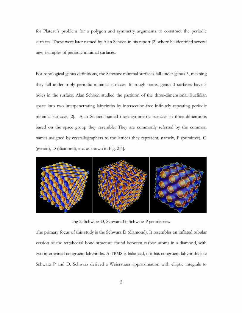
(gyroid), D (diamond), etc. as shown in Fig. 2[4].
Fig 2: Schwarz D, Schwarz G, Schwarz P geometries.
The primary focus of this study is the Schwarz D (diamond). It resembles an inflated tubular
version of the tetrahedral bond structure found between carbon atoms in a diamond, with
two intertwined congruent labyrinths. A TPMS is balanced, if it has congruent labyrinths like
Schwarz P and D. Schwarz derived a Weierstrass approximation with elliptic integrals to

3
define these surfaces [2]. But these integrals can be approximated to an implicit surface
defined by the following expression [2]:
sin(𝑥) sin(𝑦) sin(𝑧) + sin(𝑥) cos(𝑦) cos(𝑧) +
cos(𝑥) sin(𝑦) cos(𝑧) + cos(𝑥) cos(𝑦) sin(𝑧) = 0 (1)
This expression is commonly used while modelling and prototyping the Schwarz D
geometry. One type of Schwarz D geometry is shown in Fig. 3.
Fig. 3: A representation of a Schwarz D geometry using Mathematica.
1.2 Additive manufacturing
Additive manufacturing is a term describing any manufacturing process that builds a 3D
object by adding material layer-by-layer. The manufacturing process includes using a
computer and a 3D modelling software to model the object which is fed through to the
equipment which builds each layer to construct a 3D object.

4
Additive manufacturing offers flexibility in prototyping that is fast, cheap and easy to
manufacture. It offers a more efficient resource utilization in the manufacturing process by
minimizing material waste compared to traditional methods of manufacturing [5]. More
industries are considering additive manufacturing as a cost-effective method of
manufacturing. We can rethink established designs and processes that were dictated by
constraints due tomanufacturing.
FDM is the most common additive manufacturing method and is based on a process that
uses some form of thermoplastic polymer which turns into a liquid state and solidifies soon
after its contact with the built layer. The most common desktop 3D printers use materials
like PLA (Polylactic acid), ABS (Acrylonitrile Butadiene Styrene), HIPS (High Impact
Polystyrene), etc. These materials are inexpensive and are used for prototyping to visualize a
product. Desktop printers have a low-quality surface finish but are often great to test some
prints before printing the parts on high-end printers. In this study, the prototype printed
heat exchanger was built on an FDM printer using PLA.
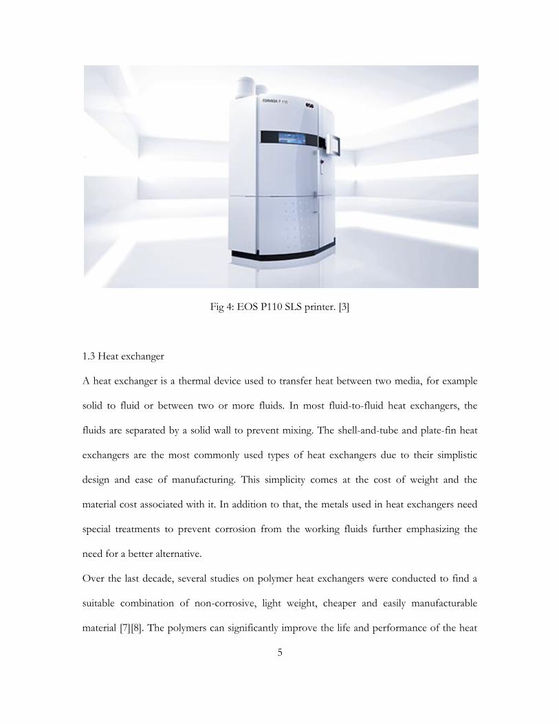
High-end printers from manufacturers like EOS (Fig.4) use another method of additive
manufacturing known as Selective Laser Sintering (SLS), more specifically a powder bed
SLS. In this process a layer of powdered material is fused into the desired shape with high
powered lasers. Unlike the FDM printers, the build is supported by the unsintered powder
from the previous layers. The material used in this study is PA 2200 – Polyamide White or
Nylon 12. It provides high detail resolution and has the highest quality of surface finish
among the polymers discussed.
5
Fig 4: EOS P110 SLS printer. [3]
1.3 Heat exchanger
A heat exchanger is a thermal device used to transfer heat between two media, for example
solid to fluid or between two or more fluids. In most fluid-to-fluid heat exchangers, the
fluids are separated by a solid wall to prevent mixing. The shell-and-tube and plate-fin heat
exchangers are the most commonly used types of heat exchangers due to their simplistic
design and ease of manufacturing. This simplicity comes at the cost of weight and the
material cost associated with it. In addition to that, the metals used in heat exchangers need
special treatments to prevent corrosion from the working fluids further emphasizing the
need for a better alternative.
Over the last decade, several studies on polymer heat exchangers were conducted to find a
suitable combination of non-corrosive, light weight, cheaper and easily manufacturable
material [7][8]. The polymers can significantly improve the life and performance of the heat
6
exchangers due to their antifouling and anticorrosive properties. Polymer heat exchangers
are lighter weight than their metal counterparts and thus reduce the costs of the heat
exchanger and the structural supportsalso become lighter [7].
Some of the studies in recent years have applied additive manufacturing technologies like 3D
printing to design and fabricate heat exchangers [7][8][9]. The common heat exchangers
found in these studies are again the familiar shell-tube and plate-fin type heat exchangers.
The study by Martinus et al. [8], on air-water straight plate-fin polymer heat exchangers
produced comparable results with a commercial product. This reinforces the need for
innovations in heat exchanger materials.
Though introduction of additive manufacturing technology offers an immense design
flexibility only a very few heat exchanger studies focus on designs other than shell-and-tube
or plate-fin. One such study is based on microfluidic membrane devices and estimates the
structure-dependent performance of microfluidic heat exchangers with sheet-like triply-
periodic minimal-surface (TPMS) architectures [9]. The TPMS geometries, namely Schawarz
P,D,G were fabricated and it was found that the Schwarz D geometry exhibited the best heat
transfer characteristics with respect to inherent pressure drop [9]. It provides the motivation
for this study which is aimed at evaluating the performance of a 3D-printed Schwarz D heat
exchanger, but on a macro rather than a micro scale.
7
CHAPTER 2
APPROACH
The present study involves testing the performance of a heat exchanger that is drastically
different from existing conventional designs. A heat exchanger is designed, built and
fabricated to conform to the triply periodic minimal surface (TPMS), with defined inlets and
outlets for the heat transfer fluids. A custom test rig is designed and built to obtain the
necessary data for all the parameters needed to analyze the performance of the system. This
section details several aspects of design considerations for both the heat exchanger and the
experimental setup.
2.1 Heat exchanger design
The heat exchanger in this study is a triply periodic minimal surface with a diamond lattice
structure known as Schwarz D. This geometry is defined by the implicit expression [2]:
sin(𝑥) sin(𝑦) sin(𝑧) + sin(𝑥) cos(𝑦) cos(𝑧) +
cos(𝑥) sin(𝑦) cos(𝑧) + cos(𝑥) cos(𝑦) sin(𝑧) = 0 (1)
We can use this equation to define the Schwarz D geometry in any mathematical plotter or
Computer Aided Design (CAD) software. Initial attempts were made to visualizing the
geometry, using MathMod ver. 5.1, of a 4-channel Schwarz D model. The software which
was great for visualizing mathematical models was limited, however, when it came to the
output file formats. The 3D printers commonly use a STL file format (abbreviated for
stereolithography, a common additive manufacturing process) which gives the raw

8
unstructured triangulated surface and normal to define a 3D object. This enables cross
platform compatibility among different types of 3D printers.
Generating these surfaces using raw data points in CAD software like SolidWorks and
Autodesk Fusion proved a bit challenging. Wolfram Mathematica, however, offers a direct
STL format geometry output from a 3D mesh plot. Using the documentation provided on
TPMS on the Wolfram Demonstrations Project [4], several modifications were made to
generate custom Schwarz D geometries in a single unit space as shown in Fig. 5 by moving
the range bar from single unit cell to any desired number of flowchannels. The visual style
and opacity of the geometry can be controlled by clicking on the respective buttons in the
dynamic evaluation window as well as the number of recursions.
9
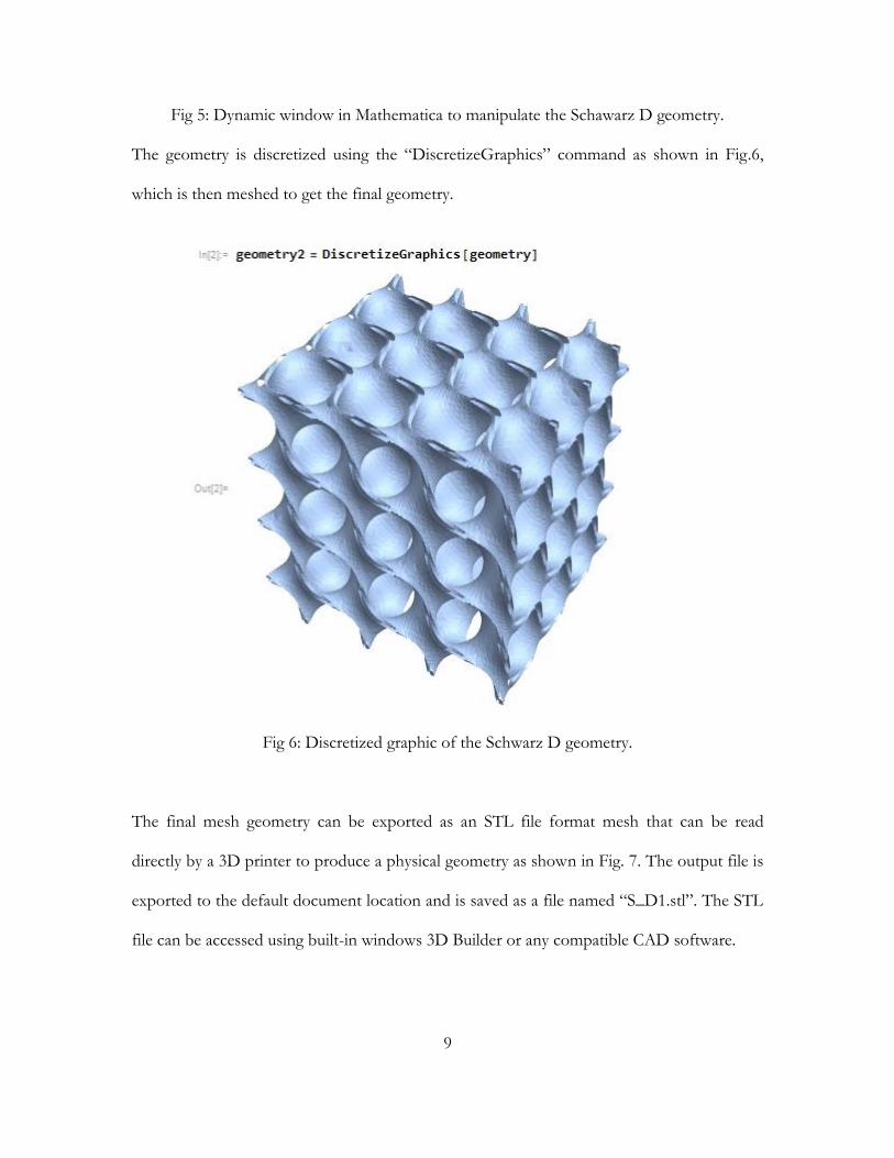
Fig 5: Dynamic window in Mathematica to manipulate the Schawarz D geometry.
The geometry is discretized using the “DiscretizeGraphics” command as shown in Fig.6,
which is then meshed to get the final geometry.
Fig 6: Discretized graphic of the Schwarz D geometry.
The final mesh geometry can be exported as an STL file format mesh that can be read
directly by a 3D printer to produce a physical geometry as shown in Fig. 7. The output file is
exported to the default document location and is saved as a file named “S_D1.stl”. The STL
file can be accessed using built-in windows 3D Builder or any compatible CAD software.

10
Fig 7: Geometry region meshed.
The geometry generated from Mathematica is an open heat exchanger without any defined
boundaries or walls or any defined inlet and outlet as seen in Fig 8. The raw format of the
STL files works to our advantage as it just defines the surfaces and not the scale of the 3D
geometry. A single file can be used to print geometries of different sizes just by updating the
dimension and scale used in that iteration. To simplify the manifolds, we can scale the
geometry to match the outer diameter of the inlet and outlet pipes for a simple geometrical
fit, in this case, 0.5in (12.7mm). This defines the scale of our heat exchanger, the inlets and
the outlets.
11
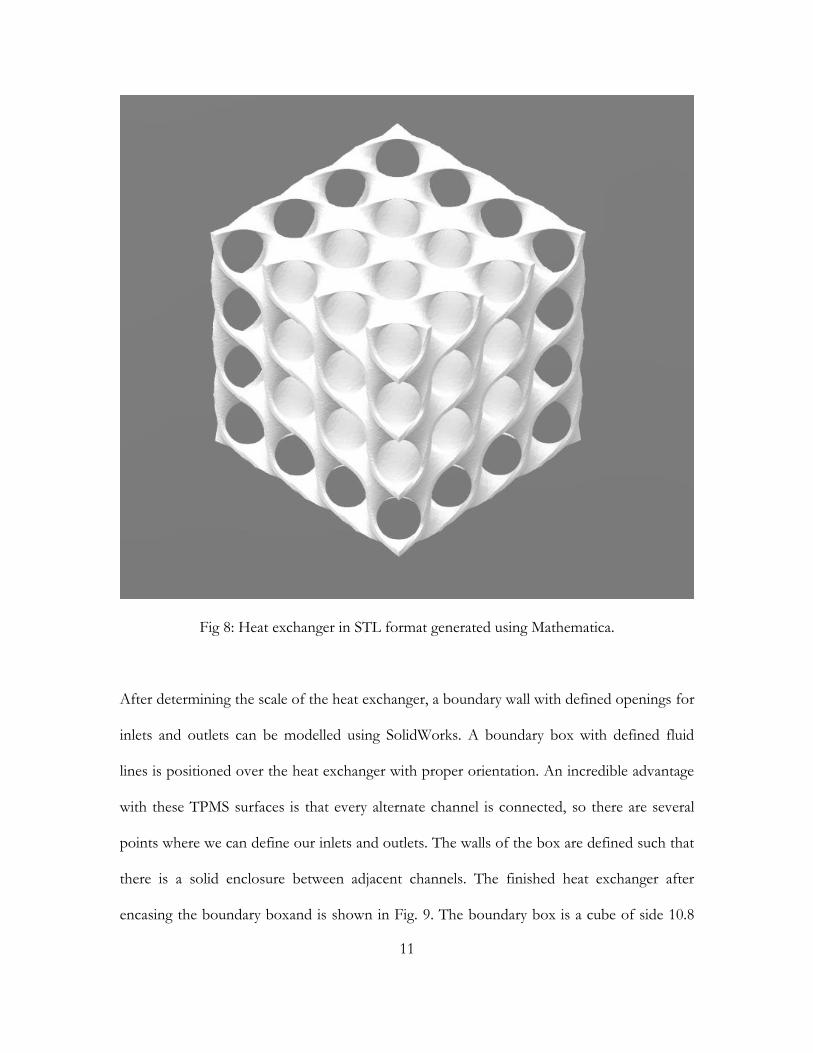
Fig 8: Heat exchanger in STL format generated using Mathematica.
After determining the scale of the heat exchanger, a boundary wall with defined openings for
inlets and outlets can be modelled using SolidWorks. A boundary box with defined fluid
lines is positioned over the heat exchanger with proper orientation. An incredible advantage
with these TPMS surfaces is that every alternate channel is connected, so there are several
points where we can define our inlets and outlets. The walls of the box are defined such that
there is a solid enclosure between adjacent channels. The finished heat exchanger after
encasing the boundary boxand is shown in Fig. 9. The boundary box is a cube of side 10.8

12
cm (4.25 in) with a thickness of 0.3 cm (0.12 in). Figure 10 shows an X-ray view of the
Schwarz geometry inside the boundary box.
Fig 9: Heat exchanger with defined fluid channels.
Fig 10: X-Ray view of the heat exchanger.
FLUID 1
FLUID 2

13
The flow paths inside the Schwarz D core can be visualized by creating a negative of the
geometry in Fig 8. The flow paths in a Schwarz D core are shown in Fig. 11.
Fig 11: Visualizing the two flow paths (red and blue) inside a Schwarz D core.
2.1.1 Fabrication
After designing the heat exchanger, we must choose a method of fabrication. As discussed
earlier, we have a variety of combinations of materials and printers we can use to print our
model. Earlier attempts to print the model using PLA extruders like MakerBot replicator
showed poor surface finish and dimensional tolerances. Finally, the model was printed using

14
PA-2200 or Polyamide, nylon 12 using an EOS P110 SLS printer by selectively sintering
layer-by-layer using a high-powered laser on a powder bed.
We focus on finding a non-dimensional parameter to quantify heat transfer effectiveness and
pressure loss for the given geometry. As a significant number of studies [7][8] have been
conducted on polymer heat exchangers the present study provides additional data to
characterize the performance of nylon-12. The fabricated model is shown in Fig. 12.
Fig 12:Fabricated Schwarz D heat exchanger
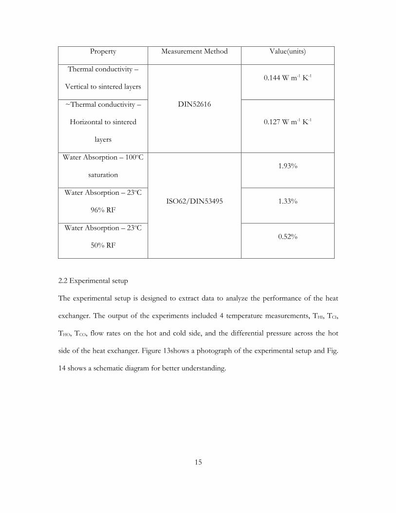
The thermal properties of Nylon-12 or PA 2200 can be found in Table 1.
Table 1: Thermal properties of Nylon-12 (PA 2200)[10]:
15
Property Measurement Method Value(units)
Thermal conductivity –
Vertical to sintered layers
DIN52616
0.144 W m-1 K-1
~Thermal conductivity –
Horizontal to sintered
layers
0.127 W m-1 K-1
Water Absorption – 100oC
saturation
ISO62/DIN53495
1.93%
Water Absorption – 23oC
96% RF 1.33%
Water Absorption – 23oC
50% RF 0.52%
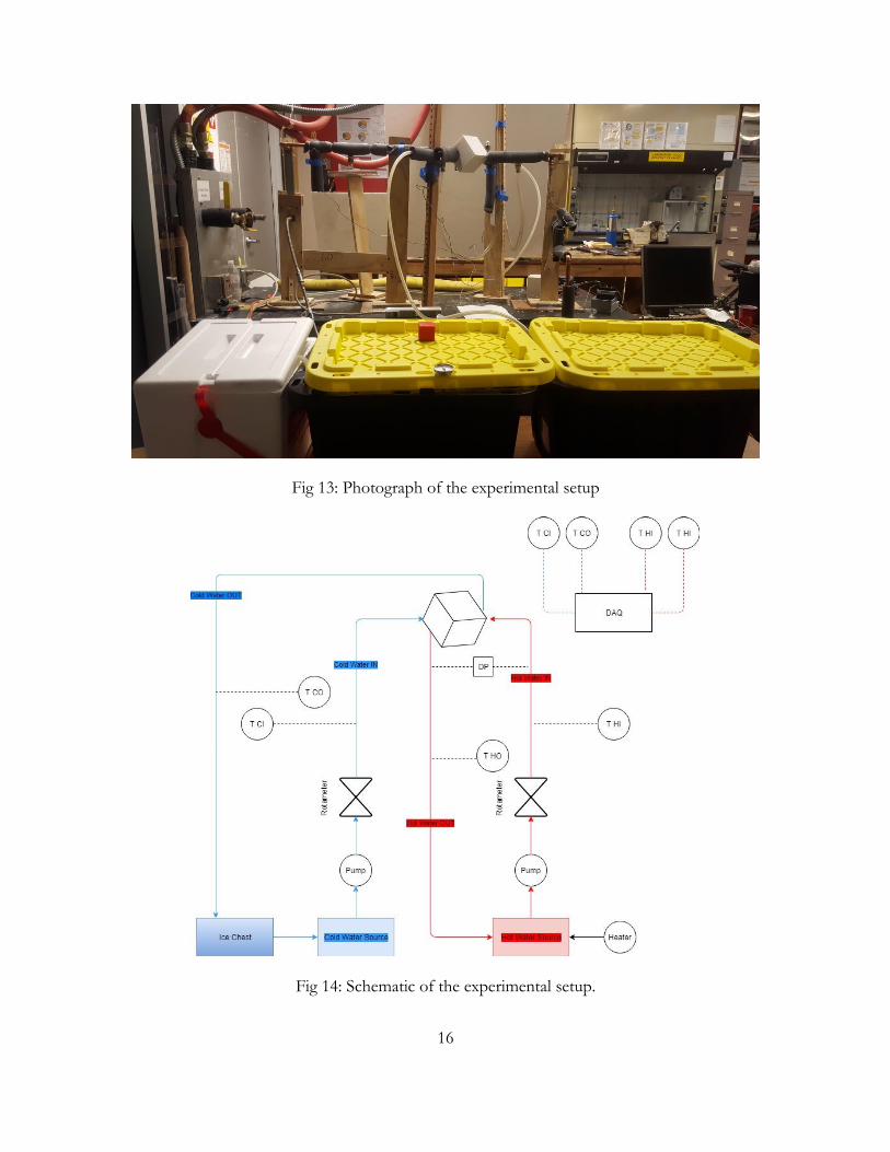
2.2 Experimental setup
The experimental setup is designed to extract data to analyze the performance of the heat
exchanger. The output of the experiments included 4 temperature measurements, THI, TCI,
THO, TCO, flow rates on the hot and cold side, and the differential pressure across the hot
side of the heat exchanger. Figure 13shows a photograph of the experimental setup and Fig.
14 shows a schematic diagram for better understanding.
16
Fig 13: Photograph of the experimental setup
Fig 14: Schematic of the experimental setup.
17
The flow must be fully developed before it enters the heat exchanger. The volume flow rates
in the experiment were regulated between 0.8 and 1.6 gpm (5.05 to 10.10 x 10⁻⁵ m3 s-1). The
flow is turbulent, Re>4000. So the entrance length is calculated using the equation [12]:
𝐿𝑒 = 4.4𝑅𝑒
1
6𝑑 (2)
where 𝐿𝑒 is the entrance length, 𝑅𝑒 the Reynolds number, and d the diameter of the inlet
pipe. For the maximum flow rate of 1.6 gpm (10.10 x 10⁻⁵ m3 s-1), 𝐿𝑒 = 26.5 𝑐𝑚.
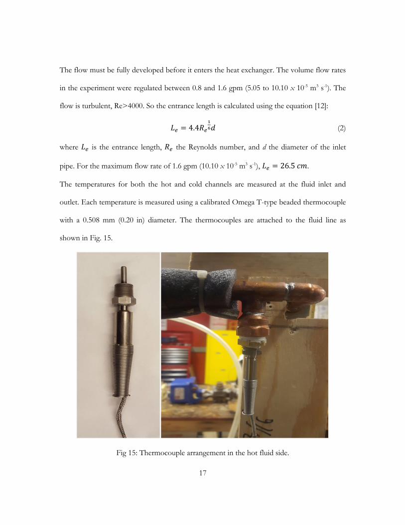
The temperatures for both the hot and cold channels are measured at the fluid inlet and
outlet. Each temperature is measured using a calibrated Omega T-type beaded thermocouple
with a 0.508 mm (0.20 in) diameter. The thermocouples are attached to the fluid line as
shown in Fig. 15.
Fig 15: Thermocouple arrangement in the hot fluid side.
18
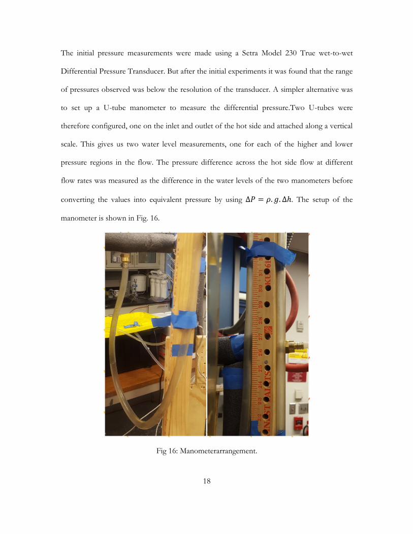
The initial pressure measurements were made using a Setra Model 230 True wet-to-wet
Differential Pressure Transducer. But after the initial experiments it was found that the range
of pressures observed was below the resolution of the transducer. A simpler alternative was
to set up a U-tube manometer to measure the differential pressure.Two U-tubes were
therefore configured, one on the inlet and outlet of the hot side and attached along a vertical
scale. This gives us two water level measurements, one for each of the higher and lower
pressure regions in the flow. The pressure difference across the hot side flow at different
flow rates was measured as the difference in the water levels of the two manometers before
converting the values into equivalent pressure by using ∆𝑃 = 𝜌. 𝑔. ∆ℎ. The setup of the
manometer is shown in Fig. 16.
Fig 16: Manometerarrangement.

19
The flow was controlled by the valves attached to the rotameters positioned on both the hot
and cold sides. The rotameters were calibrated by using the time taken to fill a graduated
3500 ml cylinder at a fixed flow rate.
The hot and cold side flows were controlled by using two pumps (EcoPlus 528 and EcoPlus
1000), where the cold side was controlled to a constant 0.8 gallon per minute(gpm) (5.05x
10-5 m3 s-1) flow rate and the hot side flow rate was regulated between 0.8 and 1.6 gpm (5.05
to 10.10x 10⁻⁵ m3 s-1)for this experiment using the knobs on the rotameter. The hot side was
heated with an immersion heater inside the reservoir. Initial trials suggested that the
temperature difference in the hot side was small enough to recirculate the water. For the
cold side, the flow was sent through an ice chest, filled with ice, before returning for
recirculation. Figure 17 shows the fluid reservoirs with marked inlets and outlets.
Fig 17: Hot and cold fluid reservoirs along with the ice chest on the cold side.
Hot Supply
Hot Return
Cold Supply
Ice Chest
Cold Return
20
The setup was built using 0.5 in (12.7 cm) copper tubing and connectors to make it uniform.
The tubes were connected using T-joints at the points where the temperature and pressure
measurements were needed. All the joints were soldered to avoid any leaks as shown in Fig.
15, with all the ends soldered.
The heat exchanger which structurally fits in to the setup is sealed using hot glue, a common
adhesive used with nylon-12 parts. Prior to data acquisition, all the exposed copper tubing
was insulated using 0.25 in (6.35 mm) foam to avoid external heat input or heat losses.
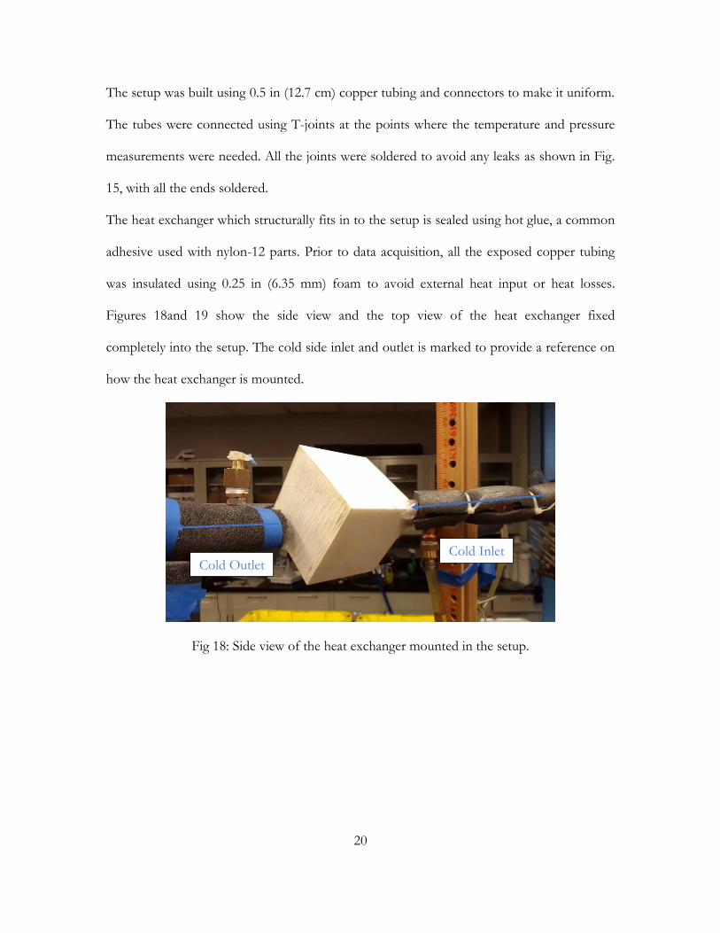
Figures 18and 19 show the side view and the top view of the heat exchanger fixed
completely into the setup. The cold side inlet and outlet is marked to provide a reference on
how the heat exchanger is mounted.
Fig 18: Side view of the heat exchanger mounted in the setup.
Cold Inlet Cold Outlet

21
Fig. 19: Top view of the heat exchanger mounted in the setup.
2.2.1 Data acquisition
The flow rate and pressure data for this experiment are measured manually by reading the
indicators in the instruments. Most of the temperature measurements, except for the
reservoir temperatures, are collected using a National Instruments (NI) NI-9213 C series
temperature input module mounted on a compact Data Acquisition (cDAQ) 9174 chassis.
We did not expect rapid temperature changes in the system, so the sampling rate was set at 1
S/s (samples/second). The thermocouples used were Omega T type beaded type
thermocouples with a 0.508 mm (0.20 in) diameter. We already established how the
thermocouples were mounted to the fluid channel in the previous section. The
thermocouples were calibrated usinga Thermo Scientific Haake DC10 P5 model thermostat,
Cold Inlet
Cold Outlet
Hot Inlet
Hot Outlet
22
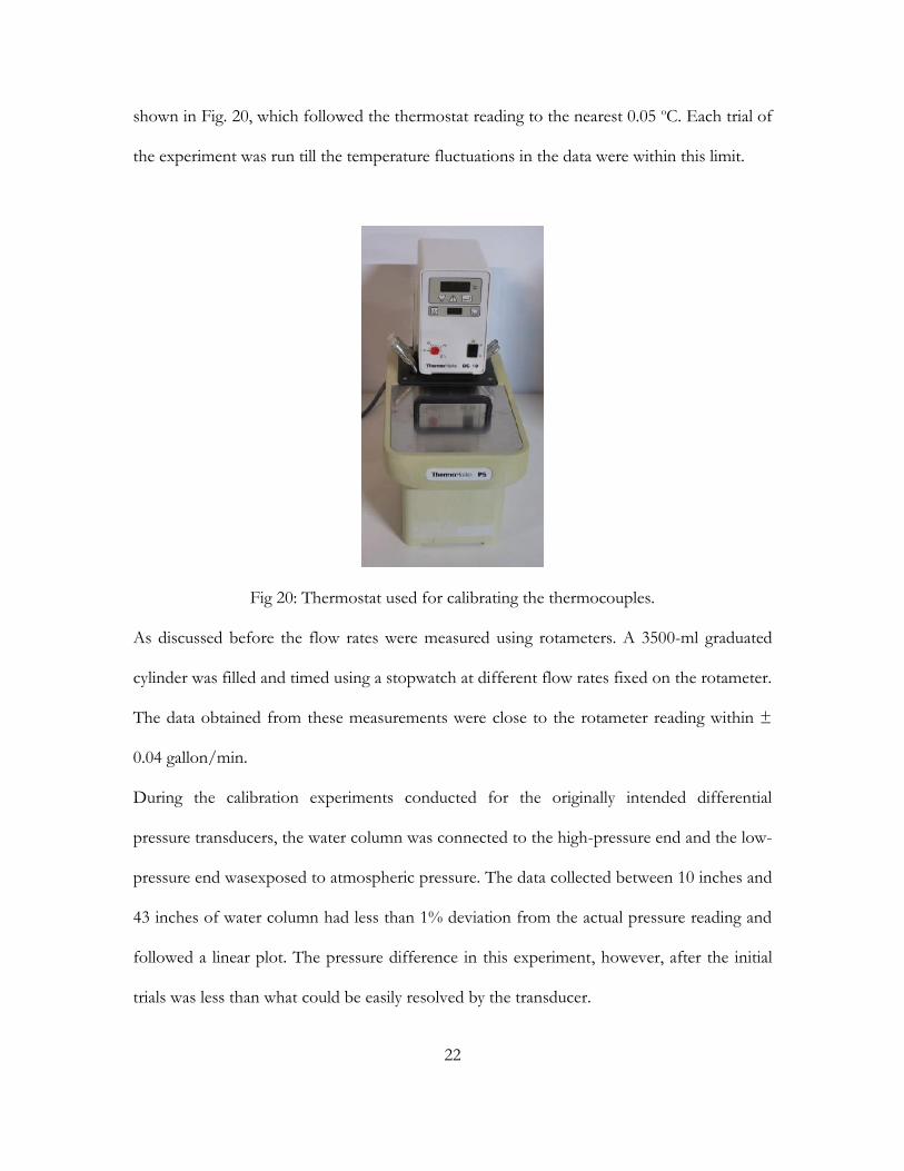
shown in Fig. 20, which followed the thermostat reading to the nearest 0.05 оC. Each trial of
the experiment was run till the temperature fluctuations in the data were within this limit.
Fig 20: Thermostat used for calibrating the thermocouples.
As discussed before the flow rates were measured using rotameters. A 3500-ml graduated
cylinder was filled and timed using a stopwatch at different flow rates fixed on the rotameter.
The data obtained from these measurements were close to the rotameter reading within ±
0.04 gallon/min.
During the calibration experiments conducted for the originally intended differential
pressure transducers, the water column was connected to the high-pressure end and the low-
pressure end wasexposed to atmospheric pressure. The data collected between 10 inches and
43 inches of water column had less than 1% deviation from the actual pressure reading and
followed a linear plot. The pressure difference in this experiment, however, after the initial
trials was less than what could be easily resolved by the transducer.
23
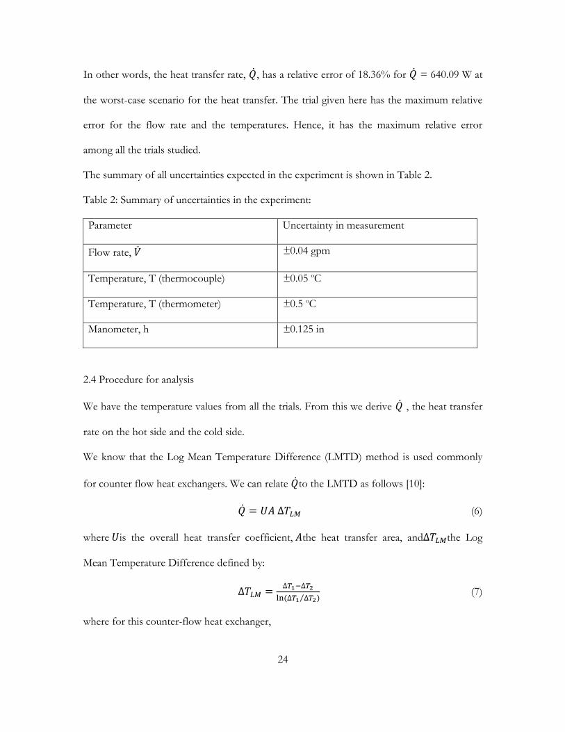
Hence, for pressure measurements we had to resort back to the U-tube manometers. The
pressure was measured by reading the length of the water column on the two manometers
on the high and low-pressure side on the hot side of the heat exchanger and noting the
difference in the height of the water column. This was compared to the standard inches of
water to psi chart to get the pressure difference. In the worst-case scenario, our error in
pressure measurement was between±8%, if the readings were misread.
2.3 Errors and uncertainties
As discussed in the previous section, our measurements have certain errors compared to the
actual value. We can use the concepts from R.J Moffat’s work on Uncertainty Analysis to
determine the uncertainties in this experiment [12]. From the data obtained in this
experiment, we can find the heat transferred, ��, in the cold channel, for example, by using
the following formula:
�� = ��. 𝜌. 𝐶𝑝. (𝑇𝑐𝑜 − 𝑇𝑐𝑖) (3)
where �� is the flow rate of the water,𝐶𝑝the specific heat of water,𝑇𝑐𝑖the temperature of the
water at the cold inlet, 𝑇𝑐𝑜 the temperature of the water at the cold outlet and 𝜌 the density
of water. The cold side temperaturesare low and are susceptible to a relatively large relative
error, hence they are used to find the maximum uncertainty in measuring the heat
transferred.
The steady-state relative error for the above expression can be found using:
𝛿��
��= {(
𝛿��
𝑉)
2
+ (𝛿𝑇𝑐𝑜
𝑇𝑐𝑜)
2
+ (𝛿𝑇𝑐𝑖
𝑇𝑐𝑖)
2
}
1
2
(4)
Plugging in the average steady-state temperatures and flow rates for a giventrial yields:
𝛿��
��= {(
0.04
0.8)
2
+ (0.5
6.21)
2
+ (0.5
3.18)
2
}
1
2
(5)
24
In other words, the heat transfer rate, ��, has a relative error of 18.36% for �� = 640.09 W at
the worst-case scenario for the heat transfer. The trial given here has the maximum relative
error for the flow rate and the temperatures. Hence, it has the maximum relative error
among all the trials studied.
The summary of all uncertainties expected in the experiment is shown in Table 2.
Table 2: Summary of uncertainties in the experiment:
Parameter Uncertainty in measurement
Flow rate, �� ±0.04 gpm
Temperature, T (thermocouple) ±0.05 oC
Temperature, T (thermometer) ±0.5 oC
Manometer, h ±0.125 in
2.4 Procedure for analysis
We have the temperature values from all the trials. From this we derive �� , the heat transfer
rate on the hot side and the cold side.
We know that the Log Mean Temperature Difference (LMTD) method is used commonly
for counter flow heat exchangers. We can relate ��to the LMTD as follows [10]:
�� = 𝑈𝐴 ∆𝑇𝐿𝑀 (6)
where 𝑈is the overall heat transfer coefficient, 𝐴the heat transfer area, and∆𝑇𝐿𝑀the Log
Mean Temperature Difference defined by:
∆𝑇𝐿𝑀 =∆𝑇1−∆𝑇2
ln (∆𝑇1 ∆𝑇2⁄ ) (7)
where for this counter-flow heat exchanger,

25
∆𝑇1 = 𝑇ℎ𝑖 − 𝑇𝑐𝑜 (8)
∆𝑇2 = 𝑇ℎ𝑜 − 𝑇𝑐𝑖 (9)
We can invert Eq. 5 to determine𝑈𝐴as:
𝑈𝐴 =��
∆𝑇𝐿𝑀 (10)
The NTU or Number of Transfer Units is a non-dimensional method to characterize a heat
exchanger. NTU is defined by:
𝑁𝑇𝑈 =𝑈𝐴
(��𝐶𝑝)𝑚𝑖𝑛
(10)
Another parametercharacterizing the heat exchanger is the heat exchanger effectiveness, ε,
which is the ratio of the rate of heat transfer ��, to the maximum theoretical heat transfer,
��𝑚𝑎𝑥 [10]:
휀 =��
��𝑚𝑎𝑥 (11)
��𝑚𝑎𝑥 = (��. 𝜌. 𝐶𝑝)𝑚𝑖𝑛 . (𝑇ℎ𝑖 − 𝑇𝑐𝑖). (12)
We can use the data obtained to find a relationship between the effectiveness and the NTU.

26
CHAPTER 3
RESULTS
The data presented in this section are obtained under steady-state conditions. Steady state
refers to the state where the inlet temperatures of both the hot and cold side vary less than
±0.5oC from their respective reservoirs.At the same time the data from the thermocouples
are constant within a bandwidth of ±0.05oC for at least 30 seconds. It was observed that
steady state was achieved within 25 minutes of the start of the experiment. After each trial,
the pumps were shut off and the system was allowed to cool off for 10 minutes before the
next trial. After the trial began, the temperature data were monitored until the temperatures
approached the reservoir temperatureafter which the data were logged until they reached
steady state. At steady state an additional set of data was logged for further analysis.
3.1 Temperatures
Table 3: Average steady-state temperature data
Trial 𝑉 (ℎ𝑜𝑡)
(𝑔𝑝𝑚)
𝑇ℎ𝑖
(℃)
𝑇𝑐𝑖
(℃)
𝑇ℎ𝑜
(℃)
𝑇𝑐𝑜
(℃)
∆𝑇1
(℃)
∆𝑇2
(℃)
∆𝑇𝐿𝑀
(℃)
1 0.8 32.58 8.15 32.23 8.36 24.22 24.08 24.15
2 0.8 44.77 17.81 44.28 18.33 26.44 26.47 26.45
3 1.2 40.16 5.39 39.82 8.61 31.55 34.43 32.97
4 1.2 30.54 3.18 30.16 6.21 24.34 26.98 25.64
5 1.2 33.07 3.58 32.66 6.52 26.55 29.08 27.80
6 1.6 39.94 7.68 39.70 8.50 31.44 32.02 31.73
7 1.6 30.83 6.55 30.66 7.34 23.49 24.11 23.80
27
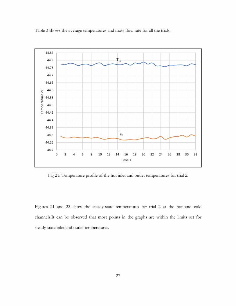
Table 3 shows the average temperatures and mass flow rate for all the trials.
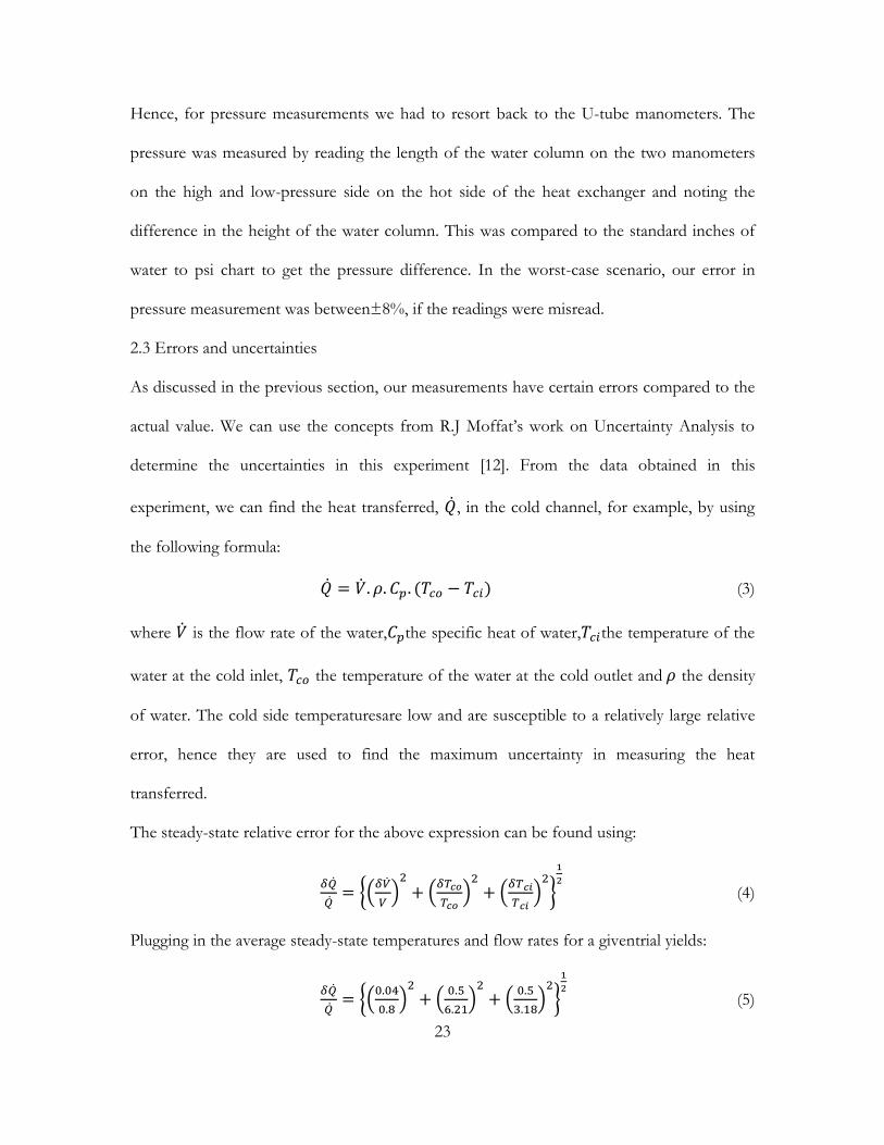
Fig 21: Temperature profile of the hot inlet and outlet temperatures for trial 2.
Figures 21 and 22 show the steady-state temperatures for trial 2 at the hot and cold
channels.It can be observed that most points in the graphs are within the limits set for
steady-state inlet and outlet temperatures.
44.2
44.25
44.3
44.35
44.4
44.45
44.5
44.55
44.6
44.65
44.7
44.75
44.8
44.85
0 2 4 6 8 10 12 14 16 18 20 22 24 26 28 30 32
Tem
per
atu
re o
C
Time s
Thi
Tho

28
Fig 22: Temperature profile of the cold inlet and outlet temperatures for trial 2.
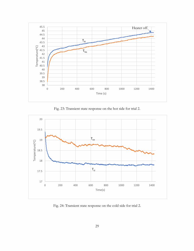
Figures 23 and 24 show the complete steady state plot for trial 2. The variance of last 40
data points in the plots are on the order of 10-4, which was considered steadystate.
17.75
17.8
17.85
17.9
17.95
18
18.05
18.1
18.15
18.2
18.25
18.3
18.35
18.4
0 2 4 6 8 10 12 14 16 18 20 22 24 26 28 30 32
Tem
per
atu
re o
C
Time s
Tco
Tci
29
Fig. 23: Transient state response on the hot side for trial 2.
Fig. 24: Transient state response on the cold side for trial 2.
38
38.5
39
39.5
40
40.5
41
41.5
42
42.5
43
43.5
44
44.5
45
45.5
0 200 400 600 800 1000 1200 1400
Tem
per
atu
re(o
C)
Time (s)
Thi
Tho
Heater off
17
17.5
18
18.5
19
19.5
20
0 200 400 600 800 1000 1200 1400
Tem
per
atu
re(o
C)
Time(s)
Tco
Tci

30
3.2 Heat Transfer Rate
Now comparing heat transferred on the hot side, the cold side and the maximum possible
heat transfer rate, we get the following result shown in Table 4. Note that the flow rate of
the cold side is fixed at 0.8 gpm (5.05 x 10⁻⁵ m3 s-1). So, the minimum heat capacity rate Cminis
always based on the cold side.
Table 4: Different heat transfer rates calculated from the data
Trial ��ℎ𝑜𝑡
(𝑊)
��𝑐𝑜𝑙𝑑
(𝑊)
��𝑚𝑎𝑥
(𝑊)
휀
=��ℎ𝑜𝑡
��𝑚𝑎𝑥
𝑈𝐴
(WK-1)
𝐶𝑚𝑖𝑛
(WK-1)
𝐶𝑚𝑎𝑥
(WK-1)
𝑁𝑇𝑈
=𝑈𝐴
𝐶𝑚𝑖𝑛
𝐶𝑚𝑖𝑛
𝐶𝑚𝑎𝑥
1 73.94
44.36 5160.85 0.0143 3.06 211.25 211.25 0.0145 1
2 103.51
109.85 5695.32 0.0182 3.91 211.25 211.25 0.0185 1
3 107.74
680.23 7345.18 0.0147 3.27 211.25 316.88 0.0155 0.67
4 120.41
640.09 5779.82 0.0208 4.70 211.25 316.88 0.0222 0.67
5 129.92
621.08 6229.78 0.0209 4.67 211.25 316.88 0.0221 0.67
6 101.40
173.22 6814.94 0.0149 3.20 211.25 422.5 0.0151 0.5
7 71.83
166.89 5129.16 0.0140 3.02 211.25 422.5 0.0143 0.5
We can observe that the heat transfer on the cold side is generally extremely high compared
to the rate of heat loss on the hot side which has a relatively consistent heat transfer rate. So,
the hot side heat transfer rate, ��ℎ𝑜𝑡 , is used to evaluate the Number of Transfer Units
(NTU). Since the temperature differences are within the uncertainty limits, the data obtained
cannot be completely trusted. This could be due to a lack of sufficient time for the heat
exchanger to attain steady-state conditions. This could also be due to the core heating up
31
and not having enough time to release the heat reflected in the cold side abnormalities. The
material nylon – 12 sometimes retains water and the retained water at a relatively higher
temperature could have sparked an anomaly in the cold side heat transfer.
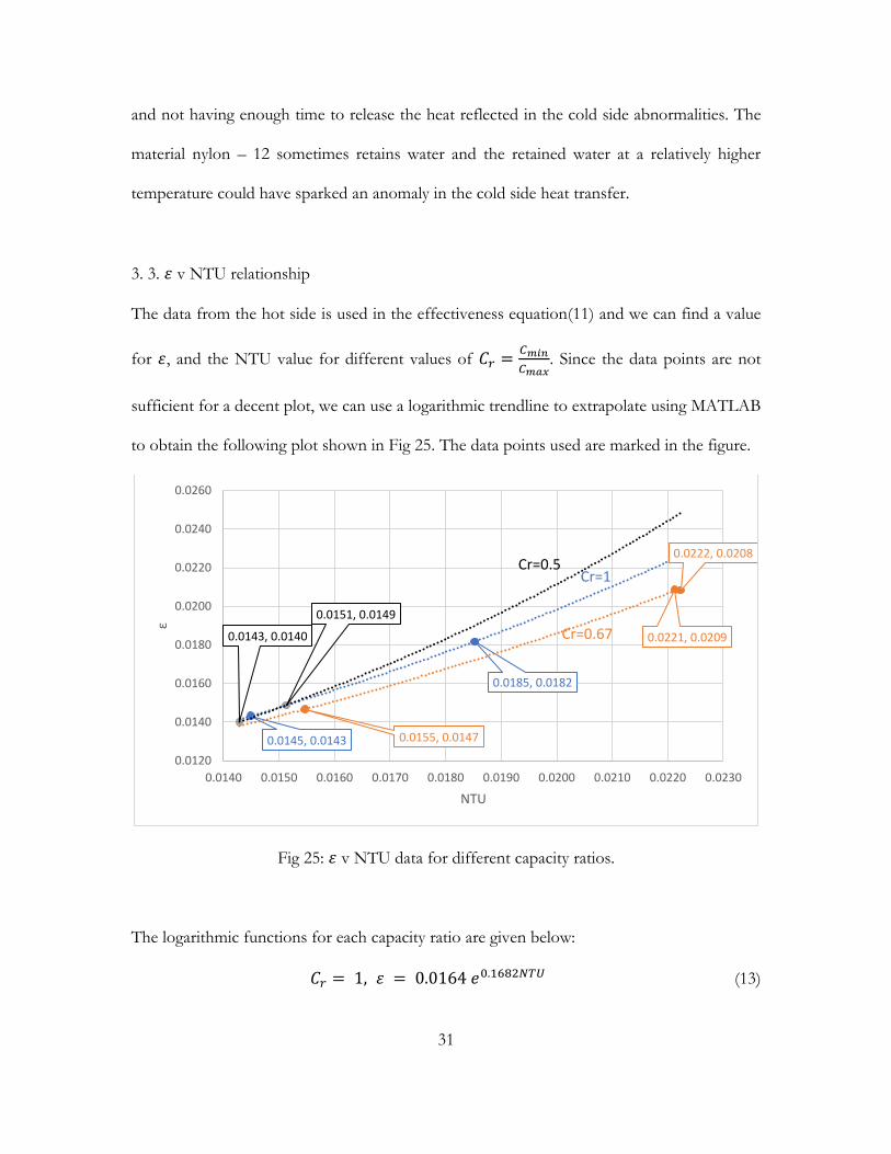
3. 3. 휀 v NTU relationship
The data from the hot side is used in the effectiveness equation(11) and we can find a value
for 휀, and the NTU value for different values of 𝐶𝑟 =𝐶𝑚𝑖𝑛
𝐶𝑚𝑎𝑥. Since the data points are not
sufficient for a decent plot, we can use a logarithmic trendline to extrapolate using MATLAB
to obtain the following plot shown in Fig 25. The data points used are marked in the figure.
Fig 25: 휀 v NTU data for different capacity ratios.
The logarithmic functions for each capacity ratio are given below:
𝐶𝑟 = 1, 휀 = 0.0164 𝑒0.1682𝑁𝑇𝑈 (13)
0.0145, 0.0143
0.0185, 0.0182
0.0155, 0.0147
0.0222, 0.0208
0.0221, 0.0209
0.0151, 0.0149
0.0143, 0.0140
0.0120
0.0140
0.0160
0.0180
0.0200
0.0220
0.0240
0.0260
0.0140 0.0150 0.0160 0.0170 0.0180 0.0190 0.0200 0.0210 0.0220 0.0230
ε
NTU
Cr=1Cr=0.5
Cr=0.67
32
𝐶𝑟 = 0.67, 휀 = 0.01854𝑒0.2025𝑁𝑇𝑈 (14)
𝐶𝑟 = 0.5, 휀 = 0.01443𝑒0.0429𝑁𝑇𝑈 (15)
The NTU values calculated for similar effectiveness values for a counter-flow shell-and-tube
heat exchanger is discussed in section 3.5
3.4. Pressure drop
Heat exchanger characterization is not complete without discussing the pressure loss across
the heat exchanger. In this experiment, we use two U tube manometers and measure
differential pressures based on the difference in heights of the two water columns. The flow
rate of the cold side is fixed at 0.8 gpm (5.05x 10⁻⁵m3 s-1) and because of the symmetry of the
heat exchanger, the pressure difference is only measured on the hot side for flow rates
between 0.8 gpm and 2.0 gpm. The differences in heights are tabulated in Table 5.
Table 5: Pressure measurements for the hot side of the heat exchanger
�� (𝑔𝑝𝑚) ∆𝐻 (𝑖𝑛) ∆𝑃 (𝑝𝑠𝑖) ∆𝑃 (𝑃𝑎)
0.8 1.625 0.059 406.79
1.2 2.625 0.095 655.00
1.6 3.500 0.126 868.74
2.0 4.125 0.149 1027.32
The plot in Fig. 26 shows the relationship between flow rate and the pressure loss.The best-
fit curve for the data obtained in the experiment is determined as
∆𝑃 = 0.0261��2 + 0.0508 RMS 0.0106 (16)

33
Fig 26: Pressure loss v flow rate in the Schwarz D heat exchanger.
The pressure loss in a pipe flow is directly related to the square of the average velocity,
∆𝑃 𝛼 𝑉2. The average velocity is proportional to the flow rate. So, we can plot a polynomial
curve of order 2 as the best-fit curve.
3.5 Comparisonto conventional heat exchangers
We can compare our results to a conventional heat exchanger in terms of material used,
effective pressure loss and performance. For this comparison we need todetermine the
hydraulic diameter of the flow. For the Schwarz D geometry, we can find the average area of
the cross section of the fluid flow by inspecting a thin cross section. The average channel
cross-sectional area is determined to be 193.69 mm2. From this the hydraulic diameter,𝐷𝐻 , is
found to be 15.72 mm. The total volume, 𝑉𝑡, occupied by the Schwarz D core is 1157.625
cm3 (cube of side 10.5 cm). The volume of material,𝑉𝑚, used for printing the heat exchanger
is 339.2 cm3. The fluid volume, 𝑉𝑓, is the difference between the two: 𝑉𝑓 = 818.425 cm3.
The total effective length of straight pipe 𝐿𝑒𝑓𝑓is found from
0.059
0.095
0.126
0.149
0.000
0.020
0.040
0.060
0.080
0.100
0.120
0.140
0.160
0.180
0.6 0.7 0.8 0.9 1 1.1 1.2 1.3 1.4 1.5 1.6 1.7 1.8 1.9 2 2.1 2.2
ΔP
(p
si)
Flow Rate (gpm)
Predicted Measured
34
𝑉𝑓 =2.𝜋.𝐷𝐻
2.𝐿𝑒𝑓𝑓
4 (17)
and is found to be 210.84 cm. The heat transfer surface area𝐴, calculated using 𝐿𝑒𝑓𝑓and 𝐷𝐻 ,
is 1040.72 cm2. For the same heat transfer surface area and hydraulic diameter, a shell-and-
tube heat exchanger core of same length will occupy a volume of 1524.53 cm3(densely
packed 20 cylinders of length 10.5 cm and 2 mm thick walls). Compared with the shell-and-
tube heat exchanger, the Schwarz D model is more compact and occupies 32% less space.
The Schwarz D geometry is equivalent to 20 tubes of length 10.5 cm with the same hydraulic
diameter, 𝐷𝐻 . We can compare the friction factor for the Schwarz D geometry, 𝑓𝐷for
different flow rates using the pipe flow friction factor equation:
𝑓𝐷 =∆𝑃𝜋2𝐷𝐻
5
32��2𝐿𝜌 (18)
The Reynolds number for the flow in the tube were found to be within the laminar region.
The friction factor for the pipe in shell-and-tube heat exchanger,𝑓𝑝 can be evaluated as [9]:
𝑓𝑝 = 64/𝑅𝑒 (18)
We can use this to evaluate a correlation factor 𝜔 for the Schwarz D geometry for laminar
flow, where,
𝑓𝐷 = 𝜔64
𝑅𝑒 (19)
The friction factors can be found in Table 7.

35
Table 7: Friction factors for Schwarz D geometry and shell-and-tube:
�� (𝑔𝑝𝑚) 𝑅𝑒 𝑓𝐷 𝑓𝑝 𝜔 =
𝑓𝐷
𝑓𝑝
0.8 229.96 178.57 0.28 637.75
1.2 344.94 127.36 0.19 670.32
1.6 459.92 95.01 0.14 678.64
2.0 574.9 71.91 0.11 653.73
Compared to the flow in a pipe, the Schwarz D geometry has a higher frictional loss if the
laminar flow case is considered. In the Schwarz D heat exchanger, geometry is a major cause
of flow disturbances due to internal mixing within the hot and cold fluid channels. Assuming
the laminar flow condition in an equivalent pipe does not consider the loss due to friction,
hence the correlation factor 𝜔 is significantly higher but are on the same order of magnitude.
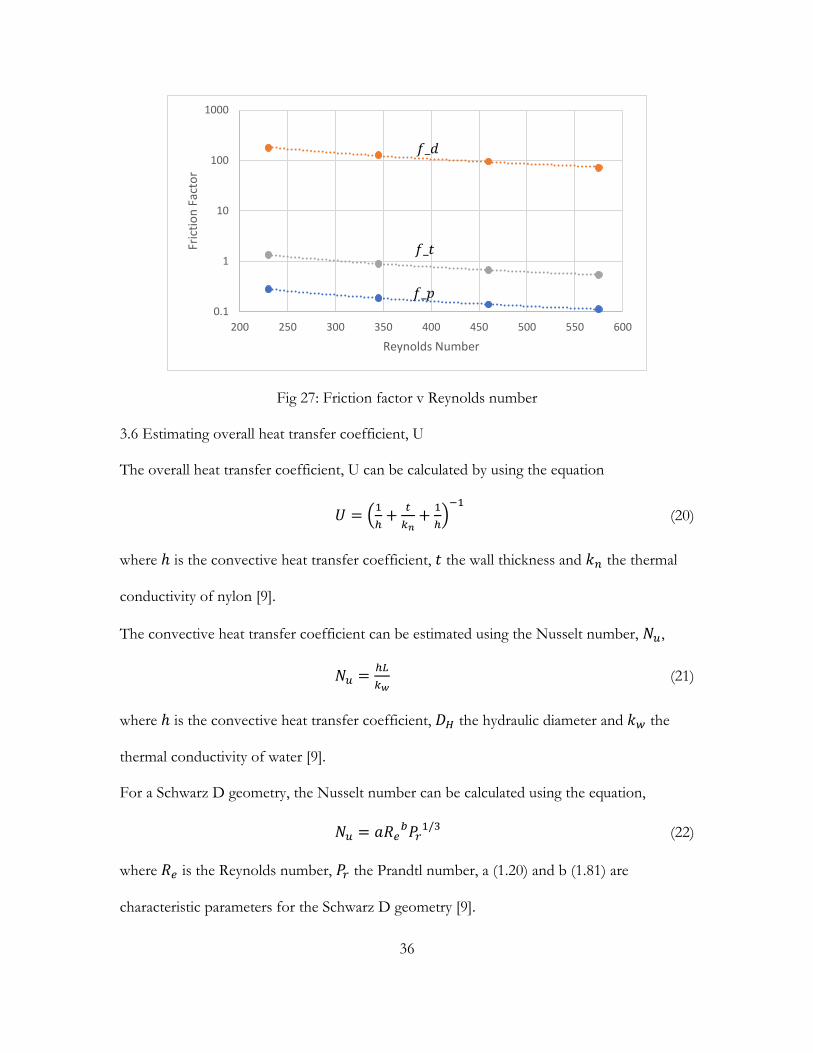
The variation friction factors for Schwarz D (𝑓𝑑)and the pipe (𝑓𝑝)compared with the
estimated friction factor from Femmer’s results (𝑓𝑡 =233
𝑅𝑒) are shown in Fig. 27.
36
Fig 27: Friction factor v Reynolds number
3.6 Estimating overall heat transfer coefficient, U
The overall heat transfer coefficient, U can be calculated by using the equation
𝑈 = (1
ℎ+
𝑡
𝑘𝑛+
1
ℎ)
−1
(20)
where ℎ is the convective heat transfer coefficient, 𝑡 the wall thickness and 𝑘𝑛 the thermal
conductivity of nylon [9].
The convective heat transfer coefficient can be estimated using the Nusselt number, 𝑁𝑢,
𝑁𝑢 =ℎ𝐿
𝑘𝑤 (21)
where ℎ is the convective heat transfer coefficient, 𝐷𝐻 the hydraulic diameter and 𝑘𝑤 the
thermal conductivity of water [9].
For a Schwarz D geometry, the Nusselt number can be calculated using the equation,
𝑁𝑢 = 𝑎𝑅𝑒𝑏𝑃𝑟
1/3 (22)
where 𝑅𝑒 is the Reynolds number, 𝑃𝑟 the Prandtl number, a (1.20) and b (1.81) are
characteristic parameters for the Schwarz D geometry [9].
0.1
1
10
100
1000
200 250 300 350 400 450 500 550 600
Fric
tio
n F
acto
r
Reynolds Number
𝑓_𝑑
𝑓_𝑝
𝑓_𝑡
37
The overall heat transfer coefficient using this method was found to be 36.1 W K-1m-2.
3.7 Discussions
The results obtained in the study were within the uncertainty limits. This can be improved
with some updates to both the heat exchanger and the experiment.
The heat exchanger wall thickness was 4 mm which can be reduced by manipulating the
thickness of the Schwarz D geometry in Mathematica. A custom python program can be
written to easily control the thickness of the geometry, which significantly improves the heat
transferred. The current design of the heat exchanger manifolds can have null spaces in the
heat exchanger where the flow is stagnated or there is no fluid flow. Increasing the number
of inlet ports can provide an evenly distributed flow pattern inside the heat exchanger. Cross
flow design provides the best flow distribution, where a single inlet can be distributed to all
available flow channels. Transparent resin-based material can be used to print the heat
exchanger for a better visual understanding of the flow. Nylon has a low thermal
conductivity, thermally conductive plastics or metal embedded plastics or even metals can be
used to print the heat exchanger for better results from the experiment.
Some changes in the experiment design can improve the results. The manifold can be
integrated into the fluid line instead of the pipes connecting into the heat exchanger for
higher operational pressures. A closed-loop temperature control drastically improves the
steady state performance, avoiding the high uncertainties in the current design by keeping
the inlet temperatures at a fixed level. Instrumentation upgrades can lower the uncertainties
in the results. The thermocouples must be mounted closer to the flow to avoid errors in
measurements due to eddies.

38
CHAPTER 4
CONCLUSION
The primary goal of this study was to try and break free from the established design norms
and explore new possibilities, taking advantage of the latest technologies like 3D printing in
thermal applications. As a first phase of this research, this study was conducted to establish
an understanding of the behavior of heat exchangers with complex 3D geometries. The
study explored several ways of generating TPMS geometries, applying different 3D printing
technologies like FDM and SLS to build prototype heat exchangers.
The experimental results show some abnormalities in the cold side for the temperatures and
the heat transfer rates. The hot side has a consistent difference across all trials. But the data
acquired are within the uncertainty limits, so no definitive conclusions can be drawn from
the data. There are several anomalies expected due to internal mixing and the geometrical
factors in this case. The steady-state from the hot side was used to determine the
effectiveness of the heat exchanger and the NTU- relation which were also within
uncertainty limits.
For same heat transfer surface area and hydraulic diameter, the volume occupied by a shell-
and-tube heat exchanger can be calculated. Compared to the shell-and-tube geometry, the
Schwarz D geometry occupies less volume and is smaller by 32%. The friction factor for the
shell-and-tube heat exchanger and the Schwarz D geometry followed similar trends, as
observed in the studies by Femmer[9], with increasing Reynolds number.

39
CHAPTER 5
FUTURE WORK
Being a relatively new area of research, a more comprehensive study should be conducted
with extensive experiments and in a more controlled environment. This would allow us to
refine the effectiveness relationships obtained by extrapolation.
Computational study needs to be done to better understand the flow paths inside the
complex geometry to help optimize the shape of the heat exchanger for better performance.
New materials like carbon/copper embedded plastics that have higher conductivity than
nylon – 12 can be used to fabricate the heat exchangers, bridging the gap between metal and
polymer heat exchangers.
40
REFERENCES
[1]Meeks III, William H., and Joaquín Pérez. "The Classical Theory Of Minimal Surfaces". Bulletin Of The American Mathematical Society, vol 48, no. 3, 2011, pp. 325-325. American Mathematical Society (AMS), doi:10.1090/s0273-0979-2011-01334-9. Accessed 23 Mar 2018. [2] NASA Electronics Research Center; Cambridge, MA, United States. Infinite Periodic
Minimal Surfaces Without Self-Intersections. 1970. Accessed 23 Mar 2018
[3] van der Net, A. (n.d.). Plateau's Memory. [Metal]. [4] Zeleny, Enrique. "Wolfram Demonstrations Project". Wolfram Demonstrations Project, 2013, http://demonstrations.wolfram.com/TriplyPeriodicMinimalSurfaces/. Accessed 23 Mar 2018. [5] Baumers, Martin et al. The Economics Of 3D Printing: A Total Cost Perspective.
Oxford, https://www.sbs.ox.ac.uk/sites/default/files/research-projects/3DP-
RDM_report.pdf. Accessed 26 Mar 2018.
[6] "FORMIGA P 110 - Laser Sintering 3D Printer – EOS". Eos.Info, 2018,
https://www.eos.info/systems_solutions/plastic/systems_equipment/formiga_p_110.
Accessed 23 Mar 2018.
[7] Chen, Xiangjie et al. "Recent Research Developments In Polymer Heat Exchangers – A
Review". Renewable And Sustainable Energy Reviews, vol 60, 2016, pp. 1367-1386. Elsevier
BV, doi:10.1016/j.rser.2016.03.024.
[8] Arie, Martinus A. et al. "Experimental Characterization Of Heat Transfer In An
Additively Manufactured Polymer Heat Exchanger". Applied Thermal Engineering, vol 113,
2017, pp. 575-584. Elsevier BV, doi:10.1016/j.applthermaleng.2016.11.030.
[9] Femmer, Tim et al. "Estimation Of The Structure Dependent Performance Of 3-D
Rapid Prototyped Membranes". Chemical Engineering Journal, vol 273, 2015, pp. 438-445.
Elsevier BV, doi:10.1016/j.cej.2015.03.029.
[10] PA2200 Product Information. EOS Gmbh - Electro Optical Systems, 2010, p. 1,
Accessed 23 Mar 2018.
[11] Cengel, Yunus A. Heat And Mass Transfer. Mcgraw-Hill, 2007.

41
[12]Moffat, R. J. "Using Uncertainty Analysis In The Planning Of An Experiment". Journal
Of Fluids Engineering, vol 107, no. 2, 1985, p. 173. ASME International,
doi:10.1115/1.3242452.

42
APPENDIX A
MATHEMATICA CODE

43
***Creates a 3D geometry Plot*** Manipulate[ geometry= ContourPlot3D[Sin[x]Sin[y]Sin[z]+Cos[x]Sin[y]Cos[z]+Cos[y]Sin[z]Cos[x]+Cos[z]Sin[x]Cos[y]==0,{x,-r,r},{y,-r,r},{z,-r,r},Axes->False,Mesh->False,Background->Black,Boxed->False,MaxRecursion->mr,Contours->1,MeshFunctions->Automatic,BoundaryStyle->If[style=="color",Directive[Yellow,Thick,Opacity[op]],None],RegionFunction->Function[{x,y,z},If[region=="cube",(True),Norm[{x,y,z}]<r]],ContourStyle->If[style=="color",{Opacity[op],Specularity[White,30],FaceForm[Orange,Blue]},{Opacity[op],Specularity[White,10],Lighting->"Neutral",Texture[ExampleData[{"Texture","Straw"}]]}],PerformanceGoal:>"Speed",ImageSize->400,SphericalRegion->True,PlotTheme->"ThickSurface"], {{r,10,"range"},1,10,ImageSize->Tiny}, {{op,.6,"opacity"},1,.3,ImageSize->Tiny}, {{mr,1,"recursion"},{0,1,2,3}}, {style,{"color","texture"}}, {region,{"cube"}},ControlPlacement->Left]
***Creates discretized points***
geometry2 = DiscretizeGraphics[geometry]
***Creates a Mesh***
geometry3 = MeshRegion[geometry2, PlotTheme -> "Lines"]
***Saves mesh as a STL file***
Export["S_D1.stl", geometry3]

44
APPENDIX B
STEADY-STATE TEMPERATURE DATA
45
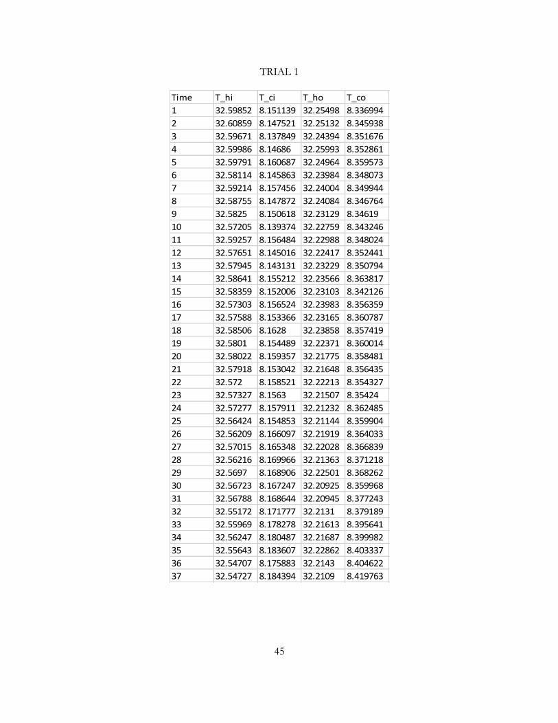
TRIAL 1
Time T_hi T_ci T_ho T_co
1 32.59852 8.151139 32.25498 8.336994
2 32.60859 8.147521 32.25132 8.345938
3 32.59671 8.137849 32.24394 8.351676
4 32.59986 8.14686 32.25993 8.352861
5 32.59791 8.160687 32.24964 8.359573
6 32.58114 8.145863 32.23984 8.348073
7 32.59214 8.157456 32.24004 8.349944
8 32.58755 8.147872 32.24084 8.346764
9 32.5825 8.150618 32.23129 8.34619
10 32.57205 8.139374 32.22759 8.343246
11 32.59257 8.156484 32.22988 8.348024
12 32.57651 8.145016 32.22417 8.352441
13 32.57945 8.143131 32.23229 8.350794
14 32.58641 8.155212 32.23566 8.363817
15 32.58359 8.152006 32.23103 8.342126
16 32.57303 8.156524 32.23983 8.356359
17 32.57588 8.153366 32.23165 8.360787
18 32.58506 8.1628 32.23858 8.357419
19 32.5801 8.154489 32.22371 8.360014
20 32.58022 8.159357 32.21775 8.358481
21 32.57918 8.153042 32.21648 8.356435
22 32.572 8.158521 32.22213 8.354327
23 32.57327 8.1563 32.21507 8.35424
24 32.57277 8.157911 32.21232 8.362485
25 32.56424 8.154853 32.21144 8.359904
26 32.56209 8.166097 32.21919 8.364033
27 32.57015 8.165348 32.22028 8.366839
28 32.56216 8.169966 32.21363 8.371218
29 32.5697 8.168906 32.22501 8.368262
30 32.56723 8.167247 32.20925 8.359968
31 32.56788 8.168644 32.20945 8.377243
32 32.55172 8.171777 32.2131 8.379189
33 32.55969 8.178278 32.21613 8.395641
34 32.56247 8.180487 32.21687 8.399982
35 32.55643 8.183607 32.22862 8.403337
36 32.54707 8.175883 32.2143 8.404622
37 32.54727 8.184394 32.2109 8.419763
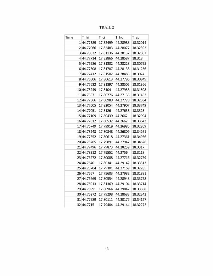
46
TRAIL 2
Time T_hi T_ci T_ho T_co
1 44.77389 17.82499 44.28988 18.32014
2 44.77066 17.82483 44.28027 18.32392
3 44.78032 17.81136 44.28137 18.32507
4 44.77714 17.82866 44.28587 18.318
5 44.76586 17.81302 44.28228 18.30795
6 44.77308 17.81787 44.28138 18.31256
7 44.77412 17.81502 44.28483 18.3074
8 44.76506 17.80613 44.27796 18.30849
9 44.77632 17.81897 44.28505 18.31366
10 44.78249 17.8104 44.27958 18.31508
11 44.76571 17.80776 44.27136 18.31452
12 44.77366 17.80989 44.27778 18.32384
13 44.77605 17.82054 44.27907 18.33749
14 44.77051 17.8126 44.27638 18.3328
15 44.77109 17.80439 44.2662 18.32994
16 44.77812 17.80532 44.2662 18.33643
17 44.76749 17.79919 44.26985 18.32869
18 44.78243 17.80848 44.26809 18.34261
19 44.77652 17.80618 44.27361 18.34936
20 44.78765 17.79891 44.27947 18.34626
21 44.77496 17.79873 44.28259 18.3317
22 44.78312 17.79552 44.2756 18.3118
23 44.76272 17.80088 44.27716 18.32759
24 44.76401 17.80341 44.29142 18.33313
25 44.75704 17.79301 44.27169 18.32785
26 44.7667 17.79603 44.27982 18.31881
27 44.76669 17.80554 44.28948 18.33758
28 44.76913 17.81369 44.29104 18.33714
29 44.76991 17.80964 44.29842 18.33588
30 44.76272 17.79298 44.28683 18.32342
31 44.77589 17.80111 44.30177 18.34127
32 44.7715 17.79484 44.29144 18.32272

47
TRIAL 3
Time T_hi T_ci T_ho T_co
1 40.18627 5.357002 39.8482 8.597448
2 40.17095 5.344331 39.84862 8.593396
3 40.17496 5.351502 39.84087 8.584881
4 40.17619 5.357128 39.84543 8.592126
5 40.16623 5.360722 39.8348 8.613932
6 40.16528 5.371623 39.83984 8.604147
7 40.17366 5.373732 39.83448 8.597951
8 40.18444 5.389389 39.84814 8.614444
9 40.1719 5.385434 39.84048 8.622361
10 40.17975 5.392693 39.84545 8.614171
11 40.16955 5.395543 39.83324 8.602315
12 40.17719 5.381581 39.83778 8.611192
13 40.17683 5.395982 39.8301 8.611042
14 40.16749 5.394048 39.83141 8.61907
15 40.17242 5.3972 39.83811 8.612962
16 40.16459 5.406192 39.8376 8.621889
17 40.17578 5.406781 39.83681 8.628869
18 40.15513 5.406266 39.82148 8.611304
19 40.16811 5.398532 39.81495 8.618548
20 40.14537 5.389078 39.81636 8.608924
21 40.15168 5.403027 39.80804 8.605009
22 40.13915 5.399083 39.80415 8.611752
23 40.14682 5.407336 39.81338 8.608339
24 40.13785 5.393624 39.80751 8.60491
25 40.1397 5.39085 39.79916 8.608077
26 40.13789 5.398207 39.80977 8.606855
27 40.13935 5.40097 39.80014 8.621206
28 40.13843 5.399978 39.79656 8.605772
29 40.13632 5.392697 39.79289 8.602095
30 40.13434 5.395334 39.79401 8.611108
31 40.1238 5.40165 39.79589 8.606721
32 40.13203 5.403824 39.80346 8.624513
33 40.12862 5.401825 39.81158 8.614475

48
TRIAL 4
Time T_hi T_ci T_ho T_co
1 30.54547 3.18222 30.16437 6.21197
2 30.58149 3.179777 30.18653 6.199272
3 30.58753 3.19266 30.19937 6.213974
4 30.57847 3.185921 30.18713 6.2149
5 30.59223 3.203636 30.19977 6.232734
6 30.57025 3.194701 30.17709 6.208857
7 30.57746 3.191091 30.18545 6.215511
8 30.5804 3.19205 30.18545 6.209082
9 30.57561 3.183128 30.18087 6.219746
10 30.5721 3.192829 30.17578 6.222476
11 30.55634 3.185699 30.17244 6.213727
12 30.57318 3.193017 30.17573 6.222187
13 30.55353 3.186556 30.16285 6.210768
14 30.54946 3.176964 30.15561 6.198384
15 30.54622 3.180005 30.15169 6.207595
16 30.5433 3.174982 30.1612 6.196414
17 30.52994 3.171599 30.14399 6.193292
18 30.52407 3.178804 30.15011 6.197591
19 30.53195 3.172531 30.15844 6.199219
20 30.53123 3.175849 30.15433 6.200371
21 30.53738 3.187646 30.16433 6.207803
22 30.53749 3.191115 30.16353 6.205295
23 30.52634 3.187922 30.15283 6.203791
24 30.53076 3.179428 30.15499 6.213213
25 30.52591 3.189144 30.15918 6.222864
26 30.51991 3.177508 30.14617 6.208926
27 30.51689 3.175502 30.14903 6.217886
28 30.52503 3.175021 30.15762 6.222886
29 30.52052 3.171916 30.15333 6.221469
30 30.50026 3.165049 30.14753 6.223221
31 30.50534 3.164922 30.14289 6.226429
32 30.50917 3.171863 30.14039 6.221178
49
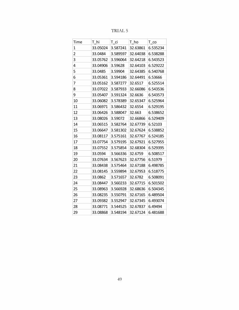
TRIAL 5
Time T_hi T_ci T_ho T_co
1 33.05024 3.587241 32.63861 6.535234
2 33.0484 3.589597 32.64038 6.538288
3 33.05762 3.596064 32.64218 6.543523
4 33.04906 3.59628 32.64103 6.529222
5 33.0485 3.59904 32.64385 6.540768
6 33.05361 3.594186 32.64491 6.53666
7 33.05162 3.587277 32.6517 6.525514
8 33.07022 3.587933 32.66086 6.543536
9 33.05407 3.591324 32.6636 6.543573
10 33.06082 3.578389 32.65347 6.525964
11 33.06971 3.586432 32.6554 6.529195
12 33.06426 3.588047 32.663 6.538652
13 33.08026 3.59072 32.66866 6.529409
14 33.06515 3.582764 32.67739 6.52103
15 33.06647 3.581302 32.67624 6.538852
16 33.08117 3.575161 32.67767 6.524185
17 33.07754 3.579195 32.67921 6.527955
18 33.07552 3.575854 32.68304 6.529395
19 33.0594 3.566336 32.6759 6.508517
20 33.07634 3.567623 32.67756 6.51979
21 33.08438 3.575464 32.67188 6.498785
22 33.08145 3.559894 32.67953 6.518775
23 33.0862 3.571657 32.6782 6.508091
24 33.08447 3.560233 32.67715 6.501502
25 33.08963 3.566928 32.68636 6.504345
26 33.08235 3.550791 32.67165 6.489504
27 33.09382 3.552947 32.67345 6.493074
28 33.08771 3.544525 32.67837 6.49494
29 33.08868 3.548194 32.67124 6.481688
50
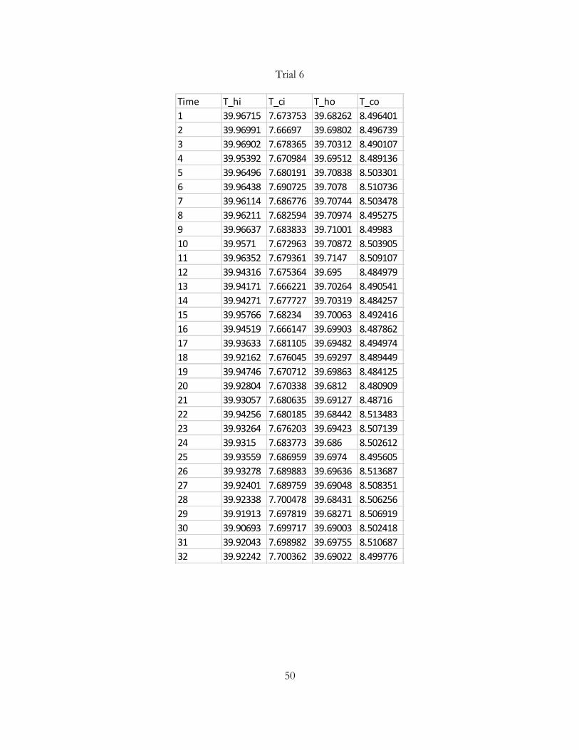
Trial 6
Time T_hi T_ci T_ho T_co
1 39.96715 7.673753 39.68262 8.496401
2 39.96991 7.66697 39.69802 8.496739
3 39.96902 7.678365 39.70312 8.490107
4 39.95392 7.670984 39.69512 8.489136
5 39.96496 7.680191 39.70838 8.503301
6 39.96438 7.690725 39.7078 8.510736
7 39.96114 7.686776 39.70744 8.503478
8 39.96211 7.682594 39.70974 8.495275
9 39.96637 7.683833 39.71001 8.49983
10 39.9571 7.672963 39.70872 8.503905
11 39.96352 7.679361 39.7147 8.509107
12 39.94316 7.675364 39.695 8.484979
13 39.94171 7.666221 39.70264 8.490541
14 39.94271 7.677727 39.70319 8.484257
15 39.95766 7.68234 39.70063 8.492416
16 39.94519 7.666147 39.69903 8.487862
17 39.93633 7.681105 39.69482 8.494974
18 39.92162 7.676045 39.69297 8.489449
19 39.94746 7.670712 39.69863 8.484125
20 39.92804 7.670338 39.6812 8.480909
21 39.93057 7.680635 39.69127 8.48716
22 39.94256 7.680185 39.68442 8.513483
23 39.93264 7.676203 39.69423 8.507139
24 39.9315 7.683773 39.686 8.502612
25 39.93559 7.686959 39.6974 8.495605
26 39.93278 7.689883 39.69636 8.513687
27 39.92401 7.689759 39.69048 8.508351
28 39.92338 7.700478 39.68431 8.506256
29 39.91913 7.697819 39.68271 8.506919
30 39.90693 7.699717 39.69003 8.502418
31 39.92043 7.698982 39.69755 8.510687
32 39.92242 7.700362 39.69022 8.499776
51
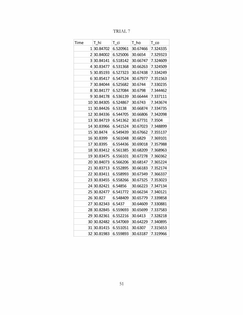
TRIAL 7
Time T_hi T_ci T_ho T_co
1 30.84702 6.520961 30.67466 7.324335
2 30.84002 6.525006 30.6654 7.329323
3 30.84141 6.518142 30.66747 7.324609
4 30.83477 6.531368 30.66263 7.324509
5 30.85193 6.527323 30.67438 7.334249
6 30.85417 6.547524 30.67977 7.351563
7 30.84044 6.525682 30.6744 7.330235
8 30.84177 6.527084 30.6798 7.344462
9 30.84178 6.536139 30.66444 7.337111
10 30.84305 6.524867 30.6743 7.343674
11 30.84426 6.53138 30.66874 7.334735
12 30.84336 6.544705 30.66806 7.342098
13 30.84719 6.541362 30.67731 7.3504
14 30.83966 6.541524 30.67023 7.348899
15 30.8474 6.549439 30.67662 7.355137
16 30.8399 6.561048 30.6829 7.369101
17 30.8395 6.554436 30.69018 7.357988
18 30.83412 6.561385 30.68209 7.368963
19 30.83475 6.556101 30.67278 7.360362
20 30.84073 6.566206 30.68147 7.365224
21 30.83713 6.552895 30.66183 7.352174
22 30.83411 6.558993 30.67349 7.366337
23 30.83455 6.558266 30.67325 7.353023
24 30.82421 6.54856 30.66223 7.347134
25 30.82477 6.541772 30.66234 7.340121
26 30.827 6.548409 30.65779 7.339858
27 30.82343 6.5437 30.64609 7.330881
28 30.82845 6.559693 30.65699 7.337583
29 30.82361 6.552216 30.6413 7.328218
30 30.82482 6.547069 30.64229 7.340895
31 30.81415 6.551051 30.6307 7.315653
32 30.81983 6.559893 30.63187 7.319966