3d simple point, topology preservation, and...

3D Simple Point, Topology Preservation, and Skeletonization

Punam Kumar SahaProfessor

Departments of ECE and RadiologyUniversity of Iowa

[email protected]

References

[1] P. K. Saha, B. Chanda, and D. D. Majumder, "Principles and algorithms for 2D and 3D shrinking,"NCKBCS Library, Indian Statistical Institute Calcutta, India, Technical Report TR/KBCS/2/91, 1991.

[2] P. K. Saha, B. B. Chaudhuri, B. Chanda, and D. D. Majumder, "Topology preservation in 3D digitalspace," Pattern Recognition, vol. 27, pp. 295-300, 1994.

[3] P. K. Saha and B. B. Chaudhuri, "Detection of 3-D simple points for topology preservingtransformations with application to thinning," IEEE Transactions on Pattern Analysis and MachineIntelligence, vol. 16, pp. 1028-1032, 1994.

[4] P. K. Saha, B. B. Chaudhuri, and D. D. Majumder, "A new shape preserving parallel thinningalgorithm for 3D digital images," Pattern Recognition, vol. 30, pp. 1939-1955, 1997.

[5] D. Jin and P. K. Saha, "A new fuzzy skeletonization algorithm and its applications to medicalimaging," Proc of the Image Analysis and Processing–ICIAP, pp. 662-671, 2013.

[6] P. K. Saha, G. Borgefors, and G. Sanniti di Baja, "A survey on skeletonization algorithms and theirapplications," Pattern Recognition Letters, 2015.

[7] P. K. Saha and B. B. Chaudhuri, "3D digital topology under binary transformation with applications,"Computer vision and image understanding, vol. 63, pp. 418-429, 1996.

[8] D. Jin, C. Chen, and P. K. Saha, "Filtering Non-Significant Quench Points Using Collision Impact inGrassfire Propagation," in Image Analysis and Processing—ICIAP 2015, Springer InternationalPublishing, pp. 432-443, 2015.

[9] D. Jin, K. S. Iyer, C. Chen, E. A. Hoffman, and P. K. Saha, "A robust and efficient curve skeletonizationalgorithm for tree-like objects using minimum cost paths," Pattern Recognition Letters, 2015.

[10] C. Chen, D. Jin, and P. K. Saha, "Fuzzy Skeletonization Improves the Performance of CharacterizingTrabecular Bone Micro-architecture," in Advances in Visual Computing, Springer InternationalPublishing, pp. 14-24, 2015.

Outline

• Introduction to topological transformation and topological equivalence

• Basic notions of digital topology• Euler characteristic• Simple point• A simple point characterization in 3-D• Number of tunnels in 3 × 3 × 3 neighborhood• Local topological numbers• Efficient algorithms• Fuzzy Skeletonization

Continuous Deformation

Continuous deformation. A transformation which shrinks, stretches, bents, twists, etc. in any way without tearing

• Envision a figure drawn on a rubber sheet

• A deformation of the sheet by stretching, twisting, bending, etc. which doesn’t tear the sheet will change the figure into some other shape

Topology. The study of those properties of geometric figures or solid bodies that remain invariant under certain transformations.

Topological Transformation and Equivalence

Topology. The study of those properties of geometric figures or solid bodies that remain invariant under certain transformations.

Topological transformation. A transformation that carries one geometric figure into another figure is a topological transformation if the following conditions are met:1) the transformation is one-to-one

2) the transformation is bicontinuous (i.e. continuous in both directions)

Topologically equivalent. Two different shapes are topologically equivalent if one can be changed to the other by a topological transformation

Basic Definitions in 3-D

26-adjacency 18-adjacency 6-adjacency

• A cubic grid constitutes the set 𝑍𝑍3

• An element of 𝑍𝑍3 is referred to as a point represented by its x-, y-, z-coordinates

• Each cube centered at an element in 𝑍𝑍3 is referred to as a voxel

Basic Definitions in 3-D

• An 𝛼𝛼-component of a set of voxels 𝑆𝑆 is a maximal subset of 𝑆𝑆 where every two voxels are 𝛼𝛼-connected in 𝑆𝑆

• An 𝛼𝛼-path 𝜋𝜋, where 𝛼𝛼 ∈ {6, 18, 26}, is a nonempty sequence 𝑝𝑝0,⋯ ,𝑝𝑝𝑙𝑙−1 of voxels where every two successive voxels are 𝛼𝛼-adjacent

26-path 6-path

Adjacency Pairs in Digital Topology

• Digital topology loosely refers to the use of mathematical topological properties and features such as connectedness, topology preservation, boundary etc., for images defined in digital grids

Jordan curve

Jordan curve

Adjacency Pairs in Digital Topology

Theorem. Jordan curve partitions of a plane into inside and outside

• Digital topology loosely refers to the use of mathematical topological properties and features such as connectedness, topology preservation, boundary etc., for images defined in digital grids

• Adjacency pairs. Rosenfeld’s approach to digital topology is to use a pair of adjacency relations 𝜅𝜅1, 𝜅𝜅0 where 𝜅𝜅1 is used for object points while 𝜅𝜅0 is used for background points

Why the Adjacency Pair?

Rosenfeld convincingly demonstrated that use of a proper adjacency pair leads to workable framework of digital topology, which holds several important mathematical topological properties, including the Jordan curve theorem

• One proper adjacency pair is (26,6)

• (26,6) is the most popular adjacency pairs in 3-D

The modern trend is to use the cubicial complex representation of digital images to define topological transformation

Cavities and Tunnels in 3-D

• Cavity. A background or white component surrounded by an object component

• Tunnel. Difficult to define a tunnel. However, the number of tunnels in an object is well-defined - the rank of the first homology group of the object.

• Intuitively, a tunnel would be the opening in the handle of a coffee mug, formed by bending a cylinder to connect the two ends to each other or to another connected object

• A hollow torus has two tunnels: the first arises from the cavity inside the ring and the second from the ring itself

Euler Characteristic

The Euler characteristic of a polyhedral set 𝑋𝑋, denoted by 𝜒𝜒(𝑋𝑋), is defined asfollows

1) 𝜒𝜒 𝜙𝜙 = 0

2) 𝜒𝜒 𝑋𝑋 = 1, if 𝑋𝑋 is non-empty and convex

3) for any two polyhedral 𝑋𝑋, 𝑌𝑌, 𝜒𝜒 𝑋𝑋 ∪ 𝑌𝑌 = 𝜒𝜒 𝑋𝑋 + 𝜒𝜒 𝑌𝑌 − 𝜒𝜒(𝑋𝑋 ∩ 𝑌𝑌)

Euler Characteristic: Alternative Definitions

The Euler characteristic of a polyhedron with each element being convex

𝜒𝜒 𝑋𝑋 = #points − #edges + #faces − #volumes,

8 ‒ 12 + 6 ‒ 1 = 1

1 ‒ 0 + 0 = 1

16 ‒ 32 + 20 ‒ 4 = 0

1 ‒ 1 + 0 = 0

and

𝜒𝜒 𝑋𝑋 = #components − #tunnels + #cavities

3-D Simple Point

Simple Point. A point whose deletion or addition preserves the topology in the local neighborhood in terms of components, tunnels, and cavities

𝑝𝑝 𝑝𝑝 𝑝𝑝

𝑝𝑝 𝑝𝑝

The major challenge. Presence of tunnels in 3-D that is not there in 2-D

3-D Simple Point Characterization by Morgenthaler (1981)

A point 𝑝𝑝 ∈ 𝑍𝑍3 is a (26,6) simple point in a 3-D binary image 𝑍𝑍3, 26,6,𝐵𝐵 if and only if the following conditions are satisfied

• In 𝑁𝑁26∗ 𝑝𝑝 , the point 𝑝𝑝 is 26-adjacent to exactly one black (object) component

• In 𝑁𝑁26∗ 𝑝𝑝 , the point 𝑝𝑝 is 6-adjacent to exactly one white (background) component

• 𝜒𝜒 𝑍𝑍3, 26,6, 𝐵𝐵 ∩ 𝑁𝑁 𝑝𝑝 ∪ 𝑝𝑝 = 𝜒𝜒 𝑍𝑍3, 26,6, 𝐵𝐵 ∩ 𝑁𝑁 𝑝𝑝 − 𝑝𝑝

𝜒𝜒 𝑋𝑋 = #components − #tunnels + #cavities

Tunnels on the Surface of a Topological Sphere

𝒮𝒮

𝐵𝐵

𝒮𝒮𝐵𝐵

• Saha, Chanda, Dutta Majumder, "Principles and algorithms for 2D and 3D shrinking," Indian Statistical Institute, Calcutta, India, TR/KBCS/2/91, 1991.• Saha, Chaudhuri, Chanda, Dutta Majumder, "Topology preservation in 3D digital space," Pat Recog, 27:295-300, 1994.• Saha and Chaudhuri, "Detection of 3-D simple points … with application to thinning," IEEE Trans Pat Anal Mach Intel, 16:1028-1032, 1994.• Saha and Chaudhuri, "3D digital topology under binary transformation with applications," Comp Vis Imag Und, 63:418-429, 1996

Tunnels on the Surface of 3x3x3 Neighborhood (Digital Case)

• In a 3 × 3 × 3 neighborhood, if the central voxel is white, all black voxels lie on its outer surface

• For computation of tunnels, a white component must be 6-adjacent to the central voxel

• Ooops still there is some problem!!


Theorem. If a voxel or point 𝑝𝑝 ∈ 𝑍𝑍3 has at a white 6-neighbor, the number oftunnels 𝜂𝜂 𝑝𝑝 in 𝑁𝑁26∗ 𝑝𝑝 is one less than the number of 6-components of whitepoints in 𝑁𝑁18∗ 𝑝𝑝 that intersect with 𝑁𝑁6∗ 𝑝𝑝 , or, zero otherwise.


3-D Simple Point Characterization by Saha et al. (1991, 1994)

A point 𝑝𝑝 ∈ 𝑍𝑍3 is a (26,6) simple point in a 3-D binary image 𝑍𝑍3, 26,6,𝐵𝐵 if and only if the following conditions are satisfied

• 𝑝𝑝 has a white (background) 6-neighbor, i.e., 𝑁𝑁6∗ 𝑝𝑝 − 𝐵𝐵 ≠ 𝜙𝜙• 𝑝𝑝 has a black (object) 26-neighbor, i.e., 𝑁𝑁26∗ 𝑝𝑝 ∩ 𝐵𝐵 ≠ 𝜙𝜙• The set of black 26-neighbors of 𝑝𝑝 is 26-connected, i.e., 𝑁𝑁26∗ 𝑝𝑝 ∩ 𝐵𝐵 is 26-connected• The set of white 6-neighbors of 𝑝𝑝 is 6-connected in the set of white 18-neighbors,

i.e., 𝑁𝑁6∗ 𝑝𝑝 − 𝐵𝐵 is 6-connected in 𝑁𝑁18∗ 𝑝𝑝 − 𝐵𝐵

Theorem. If a voxel or point 𝑝𝑝 ∈ 𝑍𝑍3 has at a white 6-neighbor, the number of tunnels𝜂𝜂 𝑝𝑝 in 𝑁𝑁26∗ 𝑝𝑝 is one less than the number of 6-components of white points in 𝑁𝑁18∗ 𝑝𝑝that intersect with 𝑁𝑁6∗ 𝑝𝑝 , or, zero otherwise.


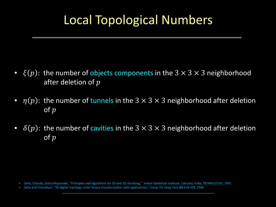
Local Topological Numbers

• 𝜉𝜉 𝑝𝑝 : the number of objects components in the 3 × 3 × 3 neighborhood after deletion of 𝑝𝑝

• 𝜂𝜂 𝑝𝑝 : the number of tunnels in the 3 × 3 × 3 neighborhood after deletion of 𝑝𝑝

• 𝛿𝛿 𝑝𝑝 : the number of cavities in the 3 × 3 × 3 neighborhood after deletion of 𝑝𝑝

• Saha, Chanda, Dutta Majumder, "Principles and algorithms for 2D and 3D shrinking," Indian Statistical Institute, Calcutta, India, TR/KBCS/2/91, 1991.• Saha and Chaudhuri, "3D digital topology under binary transformation with applications," Comp Vis Imag Und, 63:418-429, 1996

Efficient Computation of 3-D Simple Point and Local Topological Numbers

Theorem. 3-D simplicity and local topological numbers of a point is independent of its dead points.

Dead surface Dead edge


Effective Neighbors

Theorem. Object/background configuration 6-neighbors, effective e- and v-neighbors is the necessary and sufficient information to decide on 3-D simplicity and local topological numbers of a point.

• e (edge)-neighbor: 18-adjacent but not 6-adjacent, i.e., share an edge with 𝑝𝑝

• Effective e-neighbor: An e-neighbor not belonging to a dead surface

p

• v (vertex)-neighbor: 26-adjacent but not 18-adjacent, i.e., share a vertex with 𝑝𝑝

• Effective v-neighbor: A v-neighbor not belonging to a dead surface or a dead edge

p

Efficient Algorithm

• Determine the object/background configuration of 6-neighbors

• Determine the object/background configuration of effective e-neighbors

• Determine the object/background configuration of effective v-neighbors

• Use look up table to determine 3-D simplicity and the local topological numbers 𝜉𝜉 𝑝𝑝 , 𝜂𝜂(𝑝𝑝), and 𝛿𝛿 𝑝𝑝


Topology Preservation in Parallel Skeletonization

The principal challenge in topology preservation for parallel skeletonization

• a characterization of simple point guarantees topology preservation when one simple point is deleted at a time

• however, these characterizations fail to ensure topology preservation when a set of simple points are deleted in parallel

Our Approach

• Sub-iterative scheme. Divide an iteration into subiterations based on 2 × 2 × 2 subfield partitioning of the image grid

• Saha, Chaudhuri, and Dutta Majumder, "A new shape preserving parallel thinning algorithm for 3D digital images," Patt Recog, 30:1939-1955, 1997

Fuzzy Skeletonization, and its Applications

Outline

• Fuzzy Skeletonization

• Applications of Digital Topology and Geometry in Object Characterization

Principle of Skeletonization

• Object: A closed and bounded subset of R3

• Skeleton: Loci of the centers of maximal included balls

• Maximal Included Ball: A ball included in the object that cannot be cannot be fully included by another ball inside the object

• Blum’s Grassfire Transform: A process that yields the skeleton of a binary objects

Blum’s Grassfire Propagation

• Blum’s grassfire transform is defined by fire propagation on a grass field, where the field resembles a binary object.

– grassfire is simultaneously initiated at all boundary points

– grassfire propagates inwardly at a uniform speed

– the skeleton is defined as the set of quench points where two or more opposite fire fronts meet

Fuzzy Grassfire Propagation

• Fuzzy Object: A membership value is assigned at each voxel

• The membership value is interpreted as the fraction of object occupancy in a given voxel or local material density

• Fuzzy Grassfire Propagation

– grassfire is simultaneously initiated at the boundary of the support of a fuzzy object

– the speed of fire-front at at given voxel is inversely proportion to its material density, i.e., membership value

– grassfire stops at quench voxels when its natural speed of propagation is interrupted by colliding impulse from opposing fire-fronts

Outline of the Algorithm

• Primary skeletonization

‒ Locate fuzzy quench voxels in the decreasing order of FDT values and filter those using local shape factor

‒ Sequentially remove simple points that are not necessary for topology preservation in the increasing order of FDT values

• Final skeletonization

‒ Convert two-voxel thick structures into single-voxel structures

‒ Remove voxels with conflicting topological and geometric properties

• Skeleton pruning

‒ Compute global shape factor to detect spurious branches

‒ Delete spurious branches

Simple Points: Topology Preservation

Theorem: A point p is a 3-D simple point if and only if it satisfies the following four conditions:

• p has a black 26-neighbor

• p has a white 6-neighbore

• The set of black 26-neighbors of p is26-connected

• The set of white 6-neighbors of p is 6-connected in the set of white 18-neighbors of p

Simple Points: Examples

✔

✗ ✗✗

✗✔

Fuzzy Quench or Axial Points

• During fuzzy grassfire propagation, the speed of a fire-front at a given voxel equates to the inverse of local material density

• Fuzzy distance transform defines the time when the fire-front reaches at a given voxel

• This process is violated only at quench or axial points where the propagation is interrupted by colliding impulse from opposite fire-fronts

b2

a2a1

p2

b1

p1

How to Locate an Axial Point

1. Consider a shape and its axial line

2. Consider a non-axial point 𝑝𝑝1

3. Find the shortestpath 𝑝𝑝1𝑏𝑏1 toboundary

4. If we extend thepath 𝑝𝑝1𝑏𝑏1 to 𝑝𝑝2the shortest path𝑝𝑝2𝑏𝑏1 passes through 𝑝𝑝1

5. Now, consider an axial point 𝑎𝑎1

6. If extend theshortest path 𝑎𝑎1𝑏𝑏1to 𝑎𝑎2, the shortestpath from 𝑎𝑎2 to the boundary does notpasses through 𝑎𝑎1

A point 𝑎𝑎 is an axial point if there is no point 𝑎𝑎′such that a shortest path from 𝑎𝑎′ to the boundary passes through 𝑎𝑎

Fuzzy Quench or Axial Points • A point 𝑝𝑝 is a quench or axial point if there is no point 𝑝𝑝′ such that a

shortest path from 𝑝𝑝′ to the boundary passes through 𝑝𝑝.

• Specifically, a point 𝑝𝑝 is a quench or axial point if there is no point 𝑞𝑞 in the neighborhood of 𝑝𝑝 such that

Ω𝒪𝒪 𝑞𝑞 = Ω𝒪𝒪 𝑝𝑝 + 𝜇𝜇𝑑𝑑𝒪𝒪(𝑝𝑝, 𝑞𝑞)where Ω𝒪𝒪 is the FDT function and 𝜇𝜇𝑑𝑑𝒪𝒪 is the length of a link

• Arcelli, Sanniti di Baja, “Finding local maxima in a pseudo-Euclidean distance transform”, Comput Vis Graph Imag Proc, 43: 361-367, 1988• Borgefors, “Centres of maximal discs in the 5-7-11 distance transform”, Proc of the Scandinavian Conf on Imag Anal ,1: 105-105), 1993• Saha, Wehrli, “Fuzzy distance transform in general digital grids and its applications”, Proc of 7th Joint Conf Info Sc, Research Triangular Park, NC, 201-213, 2003• Svensson, “Aspects on the reverse fuzzy distance transform”, Patt Recog Lett 29: 888-896, 2008• Jin, Saha. "A new fuzzy skeletonization algorithm and its applications to medical imaging." Proc. of 17th Int Conf on Imag Anal Proc (ICIAP), 662-671, 2013.

• Arcelli and Sanniti di Baja introduced a criterion to detect the centers of maximal balls (CMBs) in a binary digital image using 3 × 3 weighted distance transform

• Borgefors extended it to 5 × 5 weighted distances• This concept was generalized to fuzzy sets by Saha and Wehrli, Svensson,

and Jin and Saha

Examples

Filtering Quench or Axial Voxels

• Too many spurious quench voxels

Support of the fuzzy object

An image slice of the fuzzy object

All quench voxels

Local Shape Factor for Quench Voxels

• At quench voxels, natural speed of fire-front propagation is interrupted by colliding impulse from opposite fire-fronts

• Local Shape Factor is defined as the measure of this “degree of colliding impulse”

• Local shape factor determines the significance of individual quench voxels

𝐿𝐿𝑆𝑆𝐿𝐿 𝑝𝑝 = 1 − 𝑓𝑓+ max𝑞𝑞∈𝑁𝑁∗ 𝑝𝑝

Ω𝒪𝒪 𝑞𝑞 − Ω𝒪𝒪 𝑝𝑝𝜇𝜇𝑑𝑑𝒪𝒪 𝑝𝑝, 𝑞𝑞

Surface and Curve Quench Voxels

• Surface Quench Voxels– two opposite fire fronts meet

• Curve Quench Voxels– fire fronts meet from all

directions on a plane

Filtering Quench Voxels

• Define a suitable support mask that fits the geometric type of the quench voxel

• Determine the significance in terms of LSF over the support mask

p p

‒ compute minimum LSF over the support mask or‒ compute the average LSF over the support mask

Support mask for a surface quench voxel

Overall significance

Filtered Axial Voxels

Support of the fuzzy object

Initial quench voxels; red voxels have lower LSF values representing noisy quench voxels

Filtered quench voxels

10Local shape factor (LSF)

Skeletal Pruning

• Compute global shape factor of each branch by adding LSF values of individual voxels and prune spurious branches

before after

A Few Examples

Evaluation

• Ground truth: High resolution 3-D binary objects with known skeletons

• Test phantoms: Down-sampling binary objects and addition of white Gaussian noise to generate fuzzy objects

low noise/blur medium noise/blur high noise/blur

Results

• Skeletons at low, medium, and high noise/blur

• Fuzzy skeletonization errors in voxel unit

Downsampling No noise SNR 24 SNR 12 SNR 63×3×3 0.49 0.52 0.54 0.584×4×4 0.52 0.53 0.54 0.585×5×5 0.57 0.58 0.59 0.60

Results of Application on Online 3D Figures

Applications

Local Thickness Computation for Fuzzy Objects

Local Width Computation for Fuzzy Objects

Fuzzy Skeletonization Improves the Sensitivity of Derived Measures

ThicknessFSK (micron)ThicknessBSK (micron)

Surface-WidthBSK (micron) Surface-WidthFSK (micron)

Yie

ld S

tress

(MPa

)

Yie

ld S

tress

(MPa

)

Yie

ld S

tress

(MPa

)

Yie

ld S

tress

(MPa

)

Summary

• The issues of sequential topological transformation in 3-D cubic grid (3-D simple point) are solved

• Local topological properties introduced by Saha et al. are useful to characterize 1-D and 2-D digital manifolds and their junctions embedded in a 3-D digital space

• Topology preservation in parallel skeletonization is effectively solved using a subfield approach

• Digital topology and geometry play important roles in medical image processing

– solves several classical problems of medical imaging

– expands the scope of target information

– provides a strong theoretical foundation to a process enhancing its stability, fidelity, and efficiency

• A comprehensive framework for fuzzy skeletonization is developed along the spirit of fuzzy grassfire propagation

• Experimental results show that the fuzzy skeletons are computed with sub-voxel accuracies under various levels of SNR and downsampling rates

• Fuzzy skeletonization improves the performance of individual trabecular thickness and width computation at in vivo CT imaging

3d simple point, topology preservation, and...

Documents