3d simulation of human-like walking and stability analysis for bipedal robot with distributed sole...
TRANSCRIPT

3D Simulation of Human-like Walking and Stability Analysis
for Bipedal Robot with Distributed Sole Force Sensors
Authors : Chao SHI and Eric H. K. FungPresenter : Dr. Eric H. K. Fung
Department of Mechanical EngineeringThe Hong Kong Polytechnic University
1

Objective :
Study the human-like walking of bipedal robot and analyze its stability with distributed force sensor model.
2
Li et al. [1] achieved a human-like walking with straightened knees, considering toe-off and heel-strike and different gait lengths.
Ogura et al. [2] achieved human-like walking with knee stretched, heel-contact and toe-off motion with robot which has a passive DoF in each foot.
The Zero Moment Point (ZMP) by Vukobratovic and Borovac [3], is used in bipedal robot stability analysis and control, regardless of different walking patterns.
3
1. Related literature

Chevallereau et al. [4] manipulates the ZMP of the bipedal robot considering the walking with foot rotation.
Nikolic et al. [5] assumed the point contact as a 2D spring-damper model and the foot ground interaction as a matrix of single point contact.
4

2. Simulation models
Features of bipedal robot :
1. Ten DoFs2. Mass property can be derived from SolidWorks3. Human-like thigh-shank length ratio
5

6
SimMechanics model for bipedal robot
Features:1. Same mass and dimensional property as physical robot2. Kinematic variables for each body part can be obtained 3. Easy to analyze its stability during walking

0 0.005 0.01 0.0150
0.25
0.5
t (s)
F n
orm
al (
N)
Point 1
Point 7Point 8
Point 22
Normal force equilibrium established for four different points
𝑭 𝐧𝐨𝐫𝐦𝐚𝐥={ 𝟎(𝜹≤𝟎)𝑲 𝜹+𝑪 �̇�(𝜹>𝟎)
7
Ground contact model
Features:1. Normal force : Spring-damper model2. Frictional force: LuGre model

For static friction and kinetic friction:
Stribeck curve can be determined by the equation :
where is the shape factor, is the Stribeck velocity and V is the relative velocity between two contacting surfaces. If , the contact can be regarded as "sticking contact".
8

At the microscopic level, the average deflection of the two surfaces z is modeled by:
where is the aggregate bristle stiffness.
Finally the LuGre friction is:
where and are damping coefficients for sticking friction and kinetic friction (viscous friction) respectively.
9
10
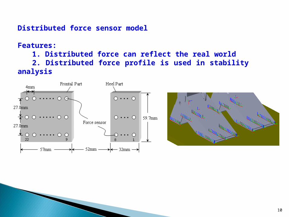
Distributed force sensor model
Features:1. Distributed force can reflect the real world2. Distributed force profile is used in stability analysis

11
Foot trajectory
Features:Three different walking phases:
heel-lifting phase swinging phase toe-striking phase
3. Simulation method

Heel-lifting phase
constraints:
Tiptoe position:
Heel position:
12

Tiptoe position:
Heel position:
13
Toe-striking phase
constraints:

𝐳=−𝟕𝟗 .𝟑𝟏𝟕𝟐𝐭 𝐬𝐰𝐢𝐧𝐠𝟓+𝟐𝟕𝟐 .𝟔𝟕𝟑𝟖𝐭𝐬𝐰𝐢𝐧𝐠
𝟒−𝟐𝟕𝟑 .𝟔𝟗𝟒𝟔𝐭 𝐬𝐰𝐢𝐧𝐠𝟑+𝟏𝟎𝟎𝐭𝐬𝐰𝐢𝐧𝐠
where is the swinging time span and .
Trajectory of swinging foot tiptoe
14
Swinging phase
The trajectory of the tiptoe in swinging phase is generated by using a fifth-order polynomial, which is sufficient to make the trajectory smooth
-100 -50 0 50 1000
20
40
x (mm)
z (m
m)

For both heel-lifting and toe-striking phase, the knees of two legs are all stretched, and for the swinging phase, only the knee from the standing leg is stretched.
Knee constraints for three walking phases:
Knee angles:
15

Trajectory of six different joints
pink: heel-lifting phase blue: swinging phase green: toe-striking phase
16
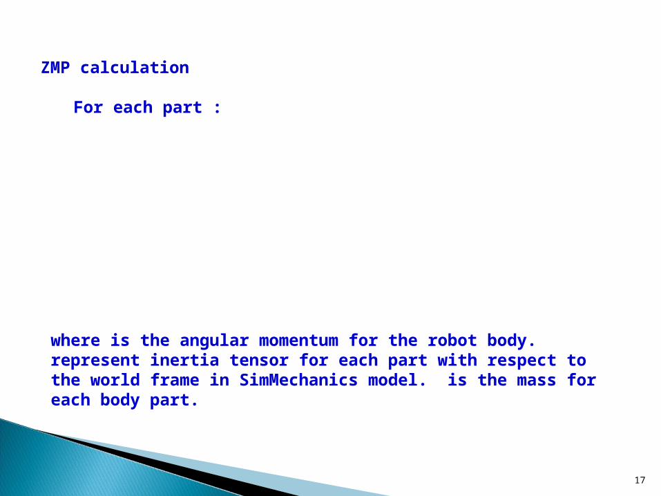
where is the angular momentum for the robot body. represent inertia tensor for each part with respect to the world frame in SimMechanics model. is the mass for each body part.
17
ZMP calculation
For each part :

ZMP for the robot body is calculated as follows :
where is the gravitational acceleration in z direction. means that the world coordinate is placed on the ground.
18

ZMP feedback mechanism
19
ZMP feedback
In the ZMP feedback block, we have following mechanism:
where and are scaling factors for heel-lifting phase and swinging phase respectively.
For small sampling time used in the simulation, the approximate equations are:
20

Overall simulation diagram
21

Snapshots of one step(a) isometric view (b) side view (c) front view
(1)-(2) : heel-lifting phase
(2)-(6): swinging phase
(6)-(7): toe-striking phase
22
4. Simulation results

Color maps of the distributed normal force during swinging phase
23
(a) (b) (c)

(a) to (b) shows the process of (2) to (3)
Force is evenly distributed along foot width direction because tilting is not severe in this period.
Pressure center moved forward along the foot length direction as the body starts to swing forward.
24
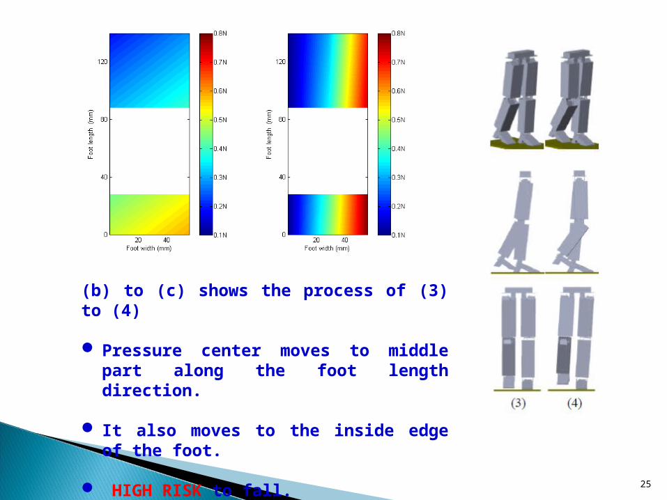
(b) to (c) shows the process of (3) to (4)
Pressure center moves to middle part along the foot length direction.
It also moves to the inside edge of the foot.
HIGH RISK to fall.
25
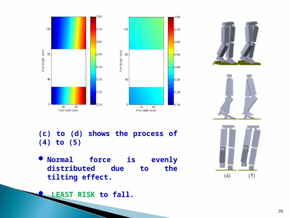
(c) to (d) shows the process of (4) to (5)
Normal force is evenly distributed due to the tilting effect.
LEAST RISK to fall.
26
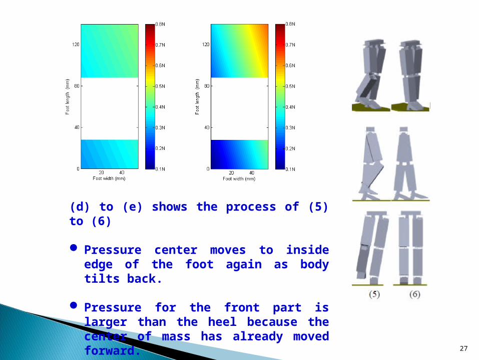
(d) to (e) shows the process of (5) to (6)
Pressure center moves to inside edge of the foot again as body tilts back.
Pressure for the front part is larger than the heel because the center of mass has already moved forward.
27

CoM and ZMP trajectory
0 100 200 300 400 500 6000
50
100
150
200
250
X(mm)
Y(m
m)
Projection of the CoM for one walking cycle( largest tilting angle )
28
0 2 4 60
200
400
600(1) CoM during one walking cycle in x direction
t(s)
CoM
x(m
m)
Right bound
Left bound
CoMx
0 2 4 60
50
100
150
200
250(2) CoM during one walking cycle in y direction
t(s)
CoM
y(m
m)
Upper bound
Lower bound
CoMy
0 2 4 60
200
400
600(1) CoM during one walking cycle in x direction
t(s)
CoM
x(m
m)
Right bound
Left bound
CoMx
0 2 4 60
50
100
150
200
250(2) CoM during one walking cycle in y direction
t(s)
CoM
y(m
m)
Upper bound
Lower bound
CoMy
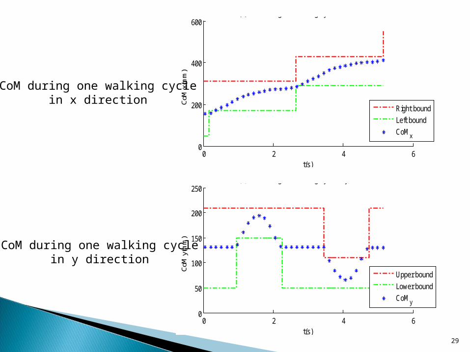
CoM during one walking cyclein x direction
CoM during one walking cyclein y direction
29

ZMP trajectory against time in one walking cycle (). Different colors represent different walking phases
pink: heel-lifting phase blue: swinging phase green: toe-striking phase
ZMP during one walking cyclein x direction
ZMP during one walking cyclein y direction
30

In this study the maximum tilting angle is taken to be for typical walking pattern.
The scaling factor is tuned until. The corresponding nominal value of, i.e. is found to be.
Different value of scaling factor can give different .
The value of can be adjusted by multiplying by the adjustment coefficient .
31
Tilting angle definition

The results are given in the following pairs :
(default)
.
0.7 0.8 0.9 1 1.1 1.2 1.3 1.48
10
12
14
16
18
adjustment coefficient
max
(deg
)
sample value
fitting curve
against adjustment coefficient
32

Trajectory of ZMPin y directionwith different
33
0 1 2 30
50
100
150
200
250
t(s)
ZM
PY
(mm
)
boundbound=0.8,
max=10.4 deg
=0.9, max
=11.7 deg
=1.0, max
=13.0 deg
=1.1, max
=14.3 deg
=1.2, max
=15.6 deg
=1.3, max
=16.9 deg
t 𝑠𝑤𝑖𝑛𝑔
t 𝑖𝑛𝑠𝑖𝑑𝑒
Percentage of swinging phase time for ZMP inside the support polygon
=

Percentage of swinging phase timefor ZMP inside the support polygon
against
Considering all cases when the ZMP is inside the upper bound, the maximum percentage is 86.69% ( and .
Walking motion with is desirable as the percentage of the swinging phase time inside the support polygon is maximum.
For, the robot walking motion will be less stable when a smaller is used.
Small will give a more human-like walking pattern.
34

5. Conclusion
With the 3D bipedal model and the ground contact model established in SimMechanics, the bipedal robot can walk stably with a given walking pattern.
The walking pattern is human-like, which includes heel-lifting phase, swinging phase and toe-striking phase.
By using the distributed force sensor model and ZMP criteria, the stability for the proposed walking pattern is successfully analyzed.
The relation between robot stability and the maximum tilting angle during swinging phase can also be obtained.
35

Acknowledgement
This research is funded by the Department of Mechanical Engineering of The Hong Kong Polytechnic University. The authors would like to thank the department for providing the facilities for this research.
36

37