3d volume reconstruction of a mouse brain from ...taoju/research/jnm_volrecon.pdf · 3d volume...
TRANSCRIPT
Journal of Neuroscience Methods xxx (2006) xxx–xxx
3D volume reconstruction of a mouse brain from histologicalsections using warp filtering
Tao Ju e,∗, Joe Warren a, James Carson f, Musodiq Bello d, Ioannis Kakadiaris d,Wah Chiu b, Christina Thaller b, Gregor Eichele c
a Rice University, Houston, TX, USAb Baylor College of Medicine, Houston, TX, USA
c Max Planck Institute of Experimental Endocrinology, Hannover, Germanyd University of Houston, Houston, TX, USA
e Washington University, St. Louis, MO, USAf Pacific Northwest National Laboratory, Richland, WA, USA
Received 28 July 2005; received in revised form 13 February 2006; accepted 13 February 2006
Abstract
wmGdtapcu©
K
1
itswsiaoe
6
0d
Sectioning tissues for optical microscopy often introduces upon the resulting sections distortions that make 3D reconstruction difficult. Heree present an automatic method for producing a smooth 3D volume from distorted 2D sections in the absence of any undistorted references. Theethod is based on pairwise elastic image warps between successive tissue sections, which can be computed by 2D image registration. Using aaussian filter, an average warp is computed for each section from the pairwise warps in a group of its neighboring sections. The average warpseform each section to match its neighboring sections, thus creating a smooth volume where corresponding features on successive sections lie closeo each other. The proposed method can be used with any existing 2D image registration method for 3D reconstruction. In particular, we present
novel image warping algorithm based on dynamic programming that extends Dynamic Time Warping in 1D speech recognition to computeairwise warps between high-resolution 2D images. The warping algorithm efficiently computes a restricted class of 2D local deformations that areharacteristic between successive tissue sections. Finally, a validation framework is proposed and applied to evaluate the quality of reconstructionsing both real sections and a synthetic volume.
2006 Elsevier B.V. All rights reserved.
eywords: 3D reconstruction; Filtering; Image warping; Dynamic programming; Histology
. Introduction
In medical imaging, volumetric data generated by 3D imag-ng methods such as MRI and CT have wide applications inhe visualization and analysis of organs. 2D imaging methods,uch as optical microscopy, typically generate serial sectionsith much higher resolution than MRI or CT scans. Recon-
truction of these 2D sections in 3D has therefore become anmportant tool for understanding anatomical structures in 3D,nd in particular, for building high-resolution templates (atlases)f organs (Timsari et al., 1999; Armstrong et al., 1995; Rosent al., 2000; Cannestra et al., 1997; MacKenzie-Graham et al.,
∗ Correspondence to: One Brookings Drive, Campus Box 1045, St. Louis, MO3130, USA. Tel.: +1 314 935 6648.
E-mail address: [email protected] (T. Ju).
2004; Sidman, 2005), or of whole animals (Brune et al., 1999).Our work is motivated by the need for automatic and efficientmethods in reconstructing, from a stack of high-resolution Nissl-stained sections, a smooth representative volume for buildinga high-quality 3D atlas of a mouse brain. Applications of theresulting atlas include visualization, physical computing, as wellas constituting a standard coordinates for mapping and com-paring brain data from different individuals. The authors havepreviously constructed a 2D atlas of the mouse brain that hasbeen successfully used to build an atlas-based database of geneexpression patterns (Ju et al., 2003).
Unfortunately, direct 3D reconstruction of serial sections bystacking successive sections will not produce a smooth vol-ume. While 3D imaging methods can be applied in vivo, planarimaging methods are applied ex vivo. The preparation stepsrequired by 2D imaging methods may introduce undesirabletissue distortions specific to the preparation procedures, which
165-0270/$ – see front matter © 2006 Elsevier B.V. All rights reserved.oi:10.1016/j.jneumeth.2006.02.020
NSM-4201; No. of Pages 17
2 T. Ju et al. / Journal of Neuroscience Methods xxx (2006) xxx–xxx
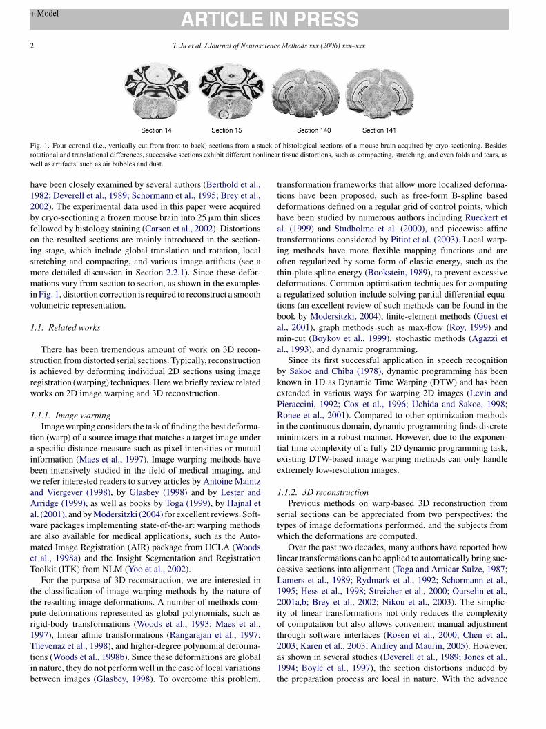
Fig. 1. Four coronal (i.e., vertically cut from front to back) sections from a stack of histological sections of a mouse brain acquired by cryo-sectioning. Besidesrotational and translational differences, successive sections exhibit different nonlinear tissue distortions, such as compacting, stretching, and even folds and tears, aswell as artifacts, such as air bubbles and dust.
have been closely examined by several authors (Berthold et al.,1982; Deverell et al., 1989; Schormann et al., 1995; Brey et al.,2002). The experimental data used in this paper were acquiredby cryo-sectioning a frozen mouse brain into 25 �m thin slicesfollowed by histology staining (Carson et al., 2002). Distortionson the resulted sections are mainly introduced in the section-ing stage, which include global translation and rotation, localstretching and compacting, and various image artifacts (see amore detailed discussion in Section 2.2.1). Since these defor-mations vary from section to section, as shown in the examplesin Fig. 1, distortion correction is required to reconstruct a smoothvolumetric representation.
1.1. Related works
There has been tremendous amount of work on 3D recon-struction from distorted serial sections. Typically, reconstructionis achieved by deforming individual 2D sections using imageregistration (warping) techniques. Here we briefly review relatedworks on 2D image warping and 3D reconstruction.
1.1.1. Image warpingImage warping considers the task of finding the best deforma-
tion (warp) of a source image that matches a target image undera specific distance measure such as pixel intensities or mutualinformation (Maes et al., 1997). Image warping methods havebwaAawameT
ttpr1Ttib
transformation frameworks that allow more localized deforma-tions have been proposed, such as free-form B-spline baseddeformations defined on a regular grid of control points, whichhave been studied by numerous authors including Rueckert etal. (1999) and Studholme et al. (2000), and piecewise affinetransformations considered by Pitiot et al. (2003). Local warp-ing methods have more flexible mapping functions and areoften regularized by some form of elastic energy, such as thethin-plate spline energy (Bookstein, 1989), to prevent excessivedeformations. Common optimisation techniques for computinga regularized solution include solving partial differential equa-tions (an excellent review of such methods can be found in thebook by Modersitzki, 2004), finite-element methods (Guest etal., 2001), graph methods such as max-flow (Roy, 1999) andmin-cut (Boykov et al., 1999), stochastic methods (Agazzi etal., 1993), and dynamic programming.
Since its first successful application in speech recognitionby Sakoe and Chiba (1978), dynamic programming has beenknown in 1D as Dynamic Time Warping (DTW) and has beenextended in various ways for warping 2D images (Levin andPieraccini, 1992; Cox et al., 1996; Uchida and Sakoe, 1998;Ronee et al., 2001). Compared to other optimization methodsin the continuous domain, dynamic programming finds discreteminimizers in a robust manner. However, due to the exponen-tial time complexity of a fully 2D dynamic programming task,existing DTW-based image warping methods can only handlee
1
stw
lcL12iot2a1t
een intensively studied in the field of medical imaging, ande refer interested readers to survey articles by Antoine Maintz
nd Viergever (1998), by Glasbey (1998) and by Lester andrridge (1999), as well as books by Toga (1999), by Hajnal et
l. (2001), and by Modersitzki (2004) for excellent reviews. Soft-are packages implementing state-of-the-art warping methods
re also available for medical applications, such as the Auto-ated Image Registration (AIR) package from UCLA (Woods
t al., 1998a) and the Insight Segmentation and Registrationoolkit (ITK) from NLM (Yoo et al., 2002).
For the purpose of 3D reconstruction, we are interested inhe classification of image warping methods by the nature ofhe resulting image deformations. A number of methods com-ute deformations represented as global polynomials, such asigid-body transformations (Woods et al., 1993; Maes et al.,997), linear affine transformations (Rangarajan et al., 1997;hevenaz et al., 1998), and higher-degree polynomial deforma-
ions (Woods et al., 1998b). Since these deformations are globaln nature, they do not perform well in the case of local variationsetween images (Glasbey, 1998). To overcome this problem,
xtremely low-resolution images.
.1.2. 3D reconstructionPrevious methods on warp-based 3D reconstruction from
erial sections can be appreciated from two perspectives: theypes of image deformations performed, and the subjects fromhich the deformations are computed.Over the past two decades, many authors have reported how
inear transformations can be applied to automatically bring suc-essive sections into alignment (Toga and Arnicar-Sulze, 1987;amers et al., 1989; Rydmark et al., 1992; Schormann et al.,995; Hess et al., 1998; Streicher et al., 2000; Ourselin et al.,001a,b; Brey et al., 2002; Nikou et al., 2003). The simplic-ty of linear transformations not only reduces the complexityf computation but also allows convenient manual adjustmenthrough software interfaces (Rosen et al., 2000; Chen et al.,003; Karen et al., 2003; Andrey and Maurin, 2005). However,s shown in several studies (Deverell et al., 1989; Jones et al.,994; Boyle et al., 1997), the section distortions induced byhe preparation process are local in nature. With the advance
T. Ju et al. / Journal of Neuroscience Methods xxx (2006) xxx–xxx 3
of image registration techniques, reconstruction methods wereproposed to correct localized section distortions by using local2D deformations (Durr et al., 1989; Guest and Baldock, 1995;Kim et al., 1997; Timsari et al., 1999; Ali and Cohen, 1998) aswell as elastic 3D surface deformations (Thompson and Toga,1996; Mega et al., 1997; Gabrani, 1998; Gefen et al., 2003).
A large number of the above reconstruction methods computethe warp of each section so that the warped section matchesa neighboring section. For example, Durr et al. (1989) com-putes elastic deformation between pairs of distorted images,while Karen et al. (2003) uses software tools for user-assistedalignment between every two consecutive sections by rigid-bodytransformations. However, unlike image registration where exactmatching is preferred, the goal of reconstruction is to form asmooth volume allowing natural progression of features throughsuccessive images (Guest and Baldock, 1995). Recent meth-ods, and in particular elastic 3D surface deformation methods,focus on warping distorted sections onto an undistorted refer-ence, such as block-face photos (Mega et al., 1997; Kim et al.,1997; Gefen et al., 2003) or tissue markers (Streicher et al.,2000; Ourselin et al., 2001b), 2D sections of a 3D in vivo image(Thompson and Toga, 1996; Schormann et al., 1995; Ourselinet al., 2001a), or sections from an existing template (He et al.,1995; Ali and Cohen, 1998; Timsari et al., 1999). The problemwith this approach is that in many applications an un-sectionedreference is not always available.
Ra2(taowtscatft((oba(i
abtomrt
the overall shape of a contoured region and has limited powerin matching interior features with neighboring sections.
1.2. Contributions
In this paper, we introduce a new approach for reconstructinga smooth representative volume by elastically deforming serialsections, which requires no human intervention or the use ofa reference volume. Since it is impossible to “undo” the tissuedistortions without the knowledge of the original object beforesectioning, we base our reconstruction on the same assumptionfrom previous works (Guest and Baldock, 1995), that is, thesection thickness (25 �m) is small comparing to variations inthe shape of anatomical structures. Instead of considering allsections at the same time (Guest and Baldock, 1995; Wirtz et al.,2004) or only two neighbors for each section (Montgomery andRoss, 1994), we consider an extended neighborhood to computethe deformation of each section. Our goal is to produce a smoothvolume where a point on a section lies close to its correspondingpoints within its neighborhood. To achieve this goal, we present:
(1) An automatic 3D reconstruction method, called warp fil-tering, based on 2D image warps between each pair ofadjacent sections. During the reconstruction, each sectionis deformed using an average warp computed from the pair-wise warps within a group of neighboring sections. The
(
oStbr
There have only been a few works so far (Montgomery andoss, 1994; Guest and Baldock, 1995; Wirtz et al., 2004) thatddress the problem of smooth 3D reconstruction using elasticD image deformations in the absence of a reference volumenote that existing methods using elastic 3D surface deforma-ions (Thompson and Toga, 1996; Mega et al., 1997; Gefen etl., 2003) cannot be applied due to the lack of a reference). With-ut the knowledge of the original object before sectioning, theseorks based their reconstruction on the following assumption:
he shape of an anatomical structure varies slowly with respect toection thickness. In other words, corresponding points on adja-ent sections are likely to be located close together. Both Guestnd Baldock (1995) and Wirtz et al. (2004) consider all sec-ions at the same time and aim at minimizing an overall energyunctional consisting of distances between every two consecu-ive sections (e.g., spring forces between corresponding pointsGuest and Baldock, 1995) or pixel-wise squared differencesWirtz et al., 2004)) and the sum of elastic deformation potentialsn every section. Although numerical solutions can be obtainedy using finite element method (Guest and Baldock, 1995) or bypproximating the differential equations using finite differencesWirtz et al., 2004), solving the global minimization problemnvolving all sections is non-trivial due to its massive size.
A completely different approach was taken by Montgomerynd Ross (1994). The idea is to reposition a point on each sectiony applying a local Laplacian smoothing operator on the posi-ion of that point and the positions of its corresponding pointsn the two adjacent sections. However, their method requiresanual delineation of contours on each section to establish cor-
espondence. Moreover, the Laplacian operator is only appliedo points on the contours, hence the deformation is restricted to
average warp results in a smooth volume by effectively repo-sitioning each point on one section to the weighted-averagelocation of the corresponding points on the neighboring sec-tions. The algorithm works with any 2D image registrationtechniques for computing pairwise warps, and can be easilyparallelized for speed. We performed quantitative and qual-itative validation of the reconstruction method on both realand synthetic data, and the results revealed the effectivenessof our method in building a smooth volume from distortedsections.
2) A new image warping algorithm based on dynamic pro-gramming for computing regularized warps between adja-cent serial sections. Due to the nature of sectioning distor-tions, we consider a class of 2D warps that can be decom-posed into 1D piecewise linear deformations with elasticconstraints. The representation of such a decomposable 2Dwarp greatly facilitates the process of warp filtering. More-over, the decomposition allows us to extend a well-known1D discrete minimization method called Dynamic TimeWarping (Sakoe and Chiba, 1978) to compute 2D elas-tic image warps even between images of high resolutions.Experimental results have shown that the proposed methodachieves an efficiency comparable to state-of-the-art warp-ing methods, while the resulting deformations often matchsuccessive tissue sections with improved accuracy.
The rest of the paper is organized as follows. We describeur image warping reconstruction algorithm in Section 2. Inection 3 we present our validation framework involving quanti-
ative measures developed from the evaluation criteria suggestedy Guest and Baldock (1995), and we report the experimentalesults on a MRI test volume and a stack of 350 histology sec-
4 T. Ju et al. / Journal of Neuroscience Methods xxx (2006) xxx–xxx
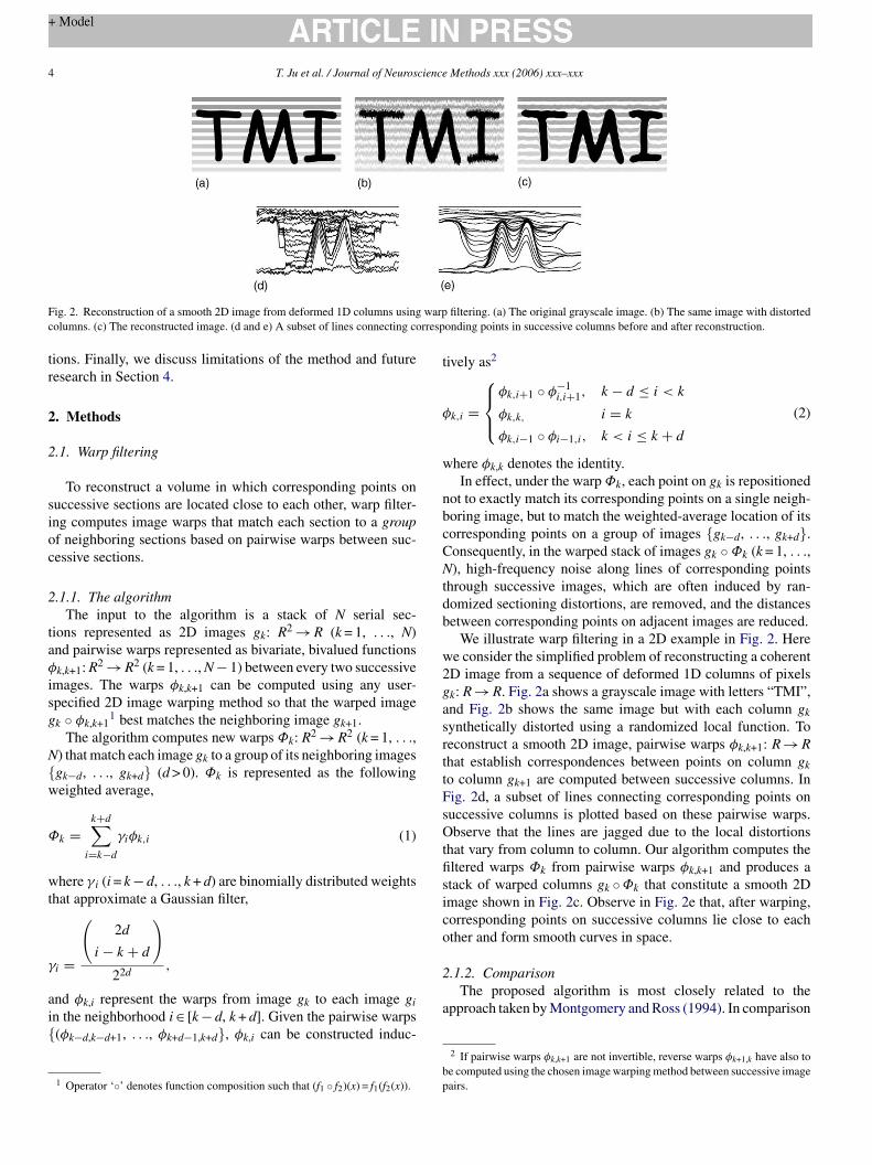
Fig. 2. Reconstruction of a smooth 2D image from deformed 1D columns using warp filtering. (a) The original grayscale image. (b) The same image with distortedcolumns. (c) The reconstructed image. (d and e) A subset of lines connecting corresponding points in successive columns before and after reconstruction.
tions. Finally, we discuss limitations of the method and futureresearch in Section 4.
2. Methods
2.1. Warp filtering
To reconstruct a volume in which corresponding points onsuccessive sections are located close to each other, warp filter-ing computes image warps that match each section to a groupof neighboring sections based on pairwise warps between suc-cessive sections.
2.1.1. The algorithmThe input to the algorithm is a stack of N serial sec-
tions represented as 2D images gk: R2 → R (k = 1, . . ., N)and pairwise warps represented as bivariate, bivalued functionsφk,k+1: R2 → R2 (k = 1, . . ., N − 1) between every two successiveimages. The warps φk,k+1 can be computed using any user-specified 2D image warping method so that the warped imagegk ◦ φk,k+1
1 best matches the neighboring image gk+1.The algorithm computes new warps Φk: R2 → R2 (k = 1, . . .,
N) that match each image gk to a group of its neighboring images{gk−d, . . ., gk+d} (d > 0). Φk is represented as the followingweighted average,
Φ
wt
γ
ai{
tively as2
φk,i =
⎧⎪⎨⎪⎩φk,i+1 ◦ φ−1
i,i+1, k − d ≤ i < k
φk,k, i = k
φk,i−1 ◦ φi−1,i, k < i ≤ k + d
(2)
where φk,k denotes the identity.In effect, under the warpΦk, each point on gk is repositioned
not to exactly match its corresponding points on a single neigh-boring image, but to match the weighted-average location of itscorresponding points on a group of images {gk−d, . . ., gk+d}.Consequently, in the warped stack of images gk ◦Φk (k = 1, . . .,N), high-frequency noise along lines of corresponding pointsthrough successive images, which are often induced by ran-domized sectioning distortions, are removed, and the distancesbetween corresponding points on adjacent images are reduced.
We illustrate warp filtering in a 2D example in Fig. 2. Herewe consider the simplified problem of reconstructing a coherent2D image from a sequence of deformed 1D columns of pixelsgk: R → R. Fig. 2a shows a grayscale image with letters “TMI”,and Fig. 2b shows the same image but with each column gksynthetically distorted using a randomized local function. Toreconstruct a smooth 2D image, pairwise warps φk,k+1: R → Rthat establish correspondences between points on column gkto column gk+1 are computed between successive columns. InFig. 2d, a subset of lines connecting corresponding points onsOtfisico
2
a
bp
k =k+d∑i=k−d
γiφk,i (1)
here γ i (i = k − d, . . ., k + d) are binomially distributed weightshat approximate a Gaussian filter,
i =
(2d
i− k + d
)
22d ,
nd φk,i represent the warps from image gk to each image gi
n the neighborhood i ∈ [k − d, k + d]. Given the pairwise warps(φk−d,k−d+1, . . ., φk+d−1,k+d}, φk,i can be constructed induc-
1 Operator ‘◦’ denotes function composition such that (f1 ◦ f2)(x) = f1(f2(x)).
uccessive columns is plotted based on these pairwise warps.bserve that the lines are jagged due to the local distortions
hat vary from column to column. Our algorithm computes theltered warps Φk from pairwise warps φk,k+1 and produces atack of warped columns gk ◦Φk that constitute a smooth 2Dmage shown in Fig. 2c. Observe in Fig. 2e that, after warping,orresponding points on successive columns lie close to eachther and form smooth curves in space.
.1.2. ComparisonThe proposed algorithm is most closely related to the
pproach taken by Montgomery and Ross (1994). In comparison
2 If pairwise warps φk,k+1 are not invertible, reverse warps φk+1,k have also toe computed using the chosen image warping method between successive imageairs.
T. Ju et al. / Journal of Neuroscience Methods xxx (2006) xxx–xxx 5
to their method, we present two major improvements. First, thecorrespondence between successive sections, which was estab-lished manually using contour lines by Montgomery and Ross(1994), is now computed automatically as image warps. Second,the simple two-neighbor Laplacian operator on contour linesis replaced by a more general de-noising Gaussian filter thatoperates on general warps between image pairs in an extendedneighborhood.
Our method also offers several unique features when com-pared to global minimization methods (Guest and Baldock,1995; Wirtz et al., 2004):
(1) Simplicity: Without the need to setup and solve a 3D min-imization problem, our local approach involves only 2Dimage warping and simple weighted-averaging operations.In general, the algorithm can be used in conjunction withany existing 2D image registration techniques for smooth3D reconstruction.
(2) Stability: In contrast with global minimization over all sec-tions, computing pairwise warps between two individualsections is a minimization problem at a small scale andtherefore less prone to errors due to variations in the inputdata. Such stability is greatly desired due to the systematicand random nature of section distortions.
(3) Efficiency: The decomposition of the reconstruction prob-lem into warping and filtering tasks makes substantial per-
2
i(w
fiu(.
c(pφ
t
•
•
•
a
many local warping methods cannot be easily adapted to takeadvantage of these function operations. In the next section, wedescribe a new image warping method for computing a local,piecewise linear warping function that is readily represented forefficient warp filtering.
2.2. Computing image warps
It is well-known that the problem of computing the optimalwarp is ill-posed (Modersitzki, 2004) and NP-complete (Keysersand Unger, 2003), hence regularization is required. For warpingbetween successive serial cryo-sectioned images, we consider aspecific type of regularized image warps such that
(1) Each 2D warp can be decomposed into a single 1D deforma-tion in the horizontal direction and independent 1D defor-mations in the vertical direction for each column, and
(2) Each 1D deformation is represented as a monotonic piece-wise linear function with elasticity constraints.
As we shall see in the following, such regularized warps arecapable of representing local deformations that are characteristicbetween adjacent serial sections. In addition, the regularizationallows fast warp filtering by supporting the three operations onwarp functions (i.e., inversion, composition and addition) ande
2
wsaArtd(
(
(
(
doccpR
φ
formance increase possible through parallelization. In par-ticular, since the pairwise warp between each image pairas well as the filtered warp for each image are computedindependently of each other, linear reduction of computa-tion time can easily be achieved in a distributed computingenvironment.
.1.3. Warp representationAlthough the warp filtering algorithm can be used with any
mage warping techniques, efficient computation using formula1) and (2) requires appropriate representation of pairwise imagearps φk,k+1.Regardless of how pairwise warps φk,k+1 are represented, the
ltered warp Φk can always be implicitly constructed by eval-ating the righthand side of formula (1) and (2) at every pointx,y). This approach, however, needs to evaluate {φk−d,k−d+1,. ., φk+d−1,k+d} for every point in the image. For efficiency, wean construct Φk as an explicit function using formula (1) and2), which can then be used to directly evaluateΦk(x,y) at everyoint (x,y). The second approach requires the pairwise warpsk,k+1 to be represented for the following operations on func-
ions:
Inversion: φ−1ij , representing the warp from image gj to image
gi.Composition: φi,j ◦φj,k, representing the warp from image gi
to image gk.Addition: aφi,j + bφi,k, representing a weighted average of thetwo warps.
Although linear functions are feasible, warps representeds higher-degree global polynomials or displacement fields in
fficient warp computation using dynamic programming.
.2.1. Decomposing 2D warpsIn our experiment (Carson et al., 2002), the frozen brain
as cut coronally into 350 cryo-sections each 25 �m thick. Tis-ue sections were placed on slides and then a Nissl stain waspplied. After staining, a coverslip was applied to each slide.ssuming that the sections have been rigidly aligned to cor-
ect the rotational and translational differences introduced whenhe tissue sections are placed on the slides (see Section 3.2 foretails), localized differences between adjacent sections includesee examples in Fig. 1):
1) Inherent anatomical variance between adjacent tissue sec-tions.
2) Regional tissue deformations in the form of vertical stretch-ing and compacting induced both during cutting and whenthe section is placed onto the slide. Extreme deformationsmay lead to tearing and folding.
3) Image artifacts, such as dust (dark artifact) and air bubbles(black ring-shaped artifact), introduced during coverslip-ping.
While the anatomical variance and image artifacts typicallyo not have specific orientation, regional distortions in the formf stretching and compacting mostly take place in the verti-al (i.e., slicing) direction. To better represent the deformationsaused by sectioning distortions while accommodating otherossible local variances, we shall compute a restricted warp φ:2 → R2 of the following form:
(x, y) = (φX(x), φY (x, y))

6 T. Ju et al. / Journal of Neuroscience Methods xxx (2006) xxx–xxx
Fig. 3. Warping from a source image (a) to a target image (b) by only com-puting the vertical deformation (c) and by computing deformations in both thehorizontal and vertical direction (d).
where φX,φY are single-valued functions. In other words, φX
models an overall 1D deformation in the horizontal direction(i.e., shifting of image columns) and φY models independent 1Ddeformations in the vertical direction for different values of x(i.e., shifting of pixels in each column). A similar decomposi-tion has been considered previously by Agazzi et al. (1993) fortext recognition. Such decomposition greatly simplifies the taskof warp computation, since 1D (vector) warps can be obtainedmuch more efficiently and robustly than 2D (image) warps.
Previous authors, such as Cox et al. (1996), have considereda more restricted form of 2D warps. In their methods, each 2Dwarp consists solely of independent 1D warps on each column(i.e., φX is the identity function). To illustrate the difference,Fig. 3 shows a simple example of warping between two imagescontaining rings of different radii, a typical type of deformationbetween successive tissue sections. Fig. 3c shows the sourceimage deformed using only 1D warps in the vertical direction,and Fig. 3d shows the same source image deformed using thecombination of 1D warps in both vertical and horizontal direc-tions. Observe that the horizontal warp φX is necessary to modelthe non-vertical variances between source and target images,which is required to handle the anatomical differences and imageartifacts in tissue sections.
2.2.2. Piecewise linear representation
oat
(
(2) The vertical deformation φY is represented by a sequence ofpiecewise linear function pairs σk, ψk: [0, L ∈ Z+] → [0, m]for k = 0, . . ., K, which match the point (σ(k),σk(l)) in images to point (ψ(k),ψk(l)) in image t for k = 0, . . ., K and l = 0,. . ., L.
We require functions σ,ψ and σ�,ψ�3 to be invertible, sothat the warp φs,t from image s to image t can be represented as:
φs,t(x, y) = (σ(x̂), σx̂(ψ−1x̂ (y)))
where x̂ = ψ−1(x) for x ∈ [0, n] and y ∈ [0, m] (linear interpola-tion is used when subscript x assumes a non-integer value). Thesymmetry of σ and ψ allows the inverse warp φt,s from imaget to image s to be represented in the same way with symbols σandψ exchanged. Such convenience will later become crucial inperforming function operations during warp filtering in Section2.2.4.
2.2.3. Elastic deformationTo prevent excessive image deformation, an image is typ-
ically modelled as an elastic material and image warps areconstrained by some form of deformation energy. Due to thepiecewise-linear nature of our warp representation, we considera discrete form of deformation energy that consists of threet
(
(
(
si
For convenient representations that will facilitate the functionperations in warp filtering, we consider 1D warps {φX, φY} thatre monotonic, piecewise linear functions. In particular, givenwo images s and t with n + 1 columns and m + 1 rows,
1) The horizontal deformation φX is represented by a pair ofpiecewise linear functions σ,ψ: [0, K ∈ Z+] → [0, n], whichmatch column σ(k) in image s to columnψ(k) in image t fork = 0, . . ., K.
erms:
1) First and second order deformation energy in the X direction:
EX(σ,ψ) = αX
K∑k=0
δ(k)2 + βX
K−1∑k=0
(δ(k + 1) − δ(k))2
where δ(k) = σ(k) −ψ(k) and αX, βX are constant weights.2) Independent first and second order deformation energy in
the Y direction for each vertical warp:
EY (σk, ψk) = αY
L∑l=0
δk(l)2 + βY
L−1∑l=0
(δk(l+ 1) − δk(l))2
where δk(l) = σk(l) −ψk(l), and αY, βY are constant weights.3) Coherence between neighboring vertical warp functions:
EC(σ�,ψ�) = γ
K−1∑k=0
L∑l=0
((σk+1(l) − σk(l))2
+ (ψk+1(l) − ψk(l))2).
where γ is a constant weight.
Note that the inclusion of the coherence term in (3) is neces-ary to ensure a smooth deformation field using a 2D warp thats decomposed into independent 1D warps.
3 σ� is the short hand for writing the whole sequence σ0, . . ., σk.
T. Ju et al. / Journal of Neuroscience Methods xxx (2006) xxx–xxx 7
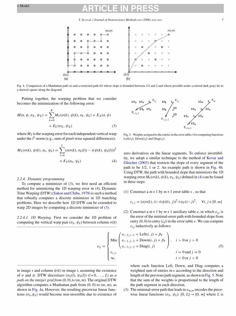
Fig. 4. Comparison of a Manhattan path (a) and a restricted path (b) whose slope is bounded between 1/2 and 2 and whose possible nodes (colored dark gray) lie ina skewed square along the diagonal.
Putting together, the warping problem that we considerbecomes the minimization of the following error:
M(σ,ψ, σ�,ψ�) =K∑k=0
MY (σ(k), ψ(k), σk, ψk) + EX(σ,ψ)
+EC(σ�,ψ�) (3)
where MY is the warping error for each independent vertical warpunder the l2-norm (e.g., sum of pixel-wise squared differences):
MY (σ(k), ψ(k), σk, ψk) =L∑l=0
(s(σ(k), σk(l)) − t(ψ(k), ψk(l)))2
+EY (σk, ψk) (4)
2.2.4. Dynamic programmingTo compute a minimizer of (3), we first need an efficient
method for minimizing the 1D warping error in (4). DynamicTime Warping (DTW) (Sakoe and Chiba, 1978) is such a methodthat robustly computes a discrete minimizer in 1D matchingproblems. Here we describe how 1D DTW can be extended towarp 2D images by computing a discrete minimizer of (3).
2.2.4.1. 1D Warping. First we consider the 1D problem ofc
iopast
Fig. 5. Weights assigned to the entries in the error table ε for computing functionsLeft(i,j), Down(i,j) and Diag(i,j).
zero derivatives on the linear segments. To enforce invertibil-ity, we adopt a similar technique to the method of Kovar andGleicher (2003) that restricts the slope of every segment of thepath to be 1/2, 1 or 2. An example path is shown in Fig. 4b.Using DTW, the path with bounded slope that minimizes the 1Dwarping error MY(σ(k),ψ(k), σk,ψk) defined in (4) can be foundin three steps:
(1) Construct a m + 1 by m + 1 error table ε , so that
εi,j = (s(σ(k), i)−t(ψ(k), j))2+αY (i−j)2, ∀i, j ∈ [0,m]
(2) Construct a m + 1 by m + 1 auxiliary table e, in which ei,j isthe error of the minimal-error path with bounded slope fromentry (0, 0) to entry (i,j) in the error table ε. We can computeei,j inductively as follows:⎛
⎜⎝ei−2,j−1 + Left(i, j) + βY
ei−1,j−2 + Down(i, j) + βY
ei−3,j−3 + Diag(i, j)
⎞⎟⎠ , i > 0 or j > 0
i = 0 and j = 0
i < 0 or j < 0
(5)
where each function Left, Down, and Diag computes aweighted sum of entries in ε according to the direction and
(
omputing the vertical warp pair (σk, ψk) between column σ(k)
n image s and column ψ(k) in image t, assuming the existencef σ and ψ. DTW discretizes (σk(l), ψk(l)) (l = 0, . . ., L) as aath on the integer grid from (0, 0) to (m, m). The original DTWlgorithm computes a Manhattan path from (0, 0) to (m, m), ashown in Fig. 4a. However, the resulting piecewise linear func-ions (σk,ψk) would become non-invertible due to existence of
eij =
⎧⎪⎪⎪⎪⎪⎪⎨⎪⎪⎪⎪⎪⎪⎩
Min
εi,j,
∞,
length of the previous path segment, as shown in Fig. 5. Notethat the sum of the weights is proportional to the length ofthe path segment in each direction.
3) The minimal-error path that leads to em,m encodes the piece-wise linear functions (σk, ψk): [0, L] → [0, m] where L is
8 T. Ju et al. / Journal of Neuroscience Methods xxx (2006) xxx–xxx
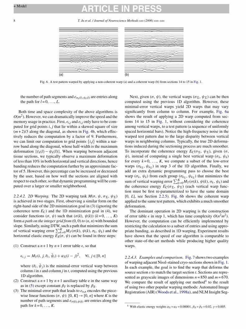
Fig. 6. A test pattern warped by applying a non-coherent warp (a) and a coherent warp (b) from sections 14 to 15 in Fig. 1.
the number of path segments and eσk(l),ψk(l) are entries alongthe path for l = 0, . . ., L.
Both time and space complexity of the above algorithms isO(m2). However, we can dramatically improve the speed and thememory usage in practice. First, εi,j and ei,j only have to be com-puted for grid points i, j that lie within a skewed square of size(m + 2)/3 along the diagonal, as shown in Fig. 4b, which effec-tively reduces the computation by a factor of 9. Furthermore,we can limit our computation to grid points {i,j} within a nar-row band along the diagonal, whose half-width is the maximumdeformation ||(k(l) −ψk(l)||. When warping between adjacenttissue sections, we typically observe a maximum deformationof less than 10% in both horizontal and vertical directions, hencebanding reduces the computation further by an approximate fac-tor of 5. However, this percentage can be increased or decreasedby the user, based on how well the sections are aligned withrespect to each other, so that dynamic programming will be com-puted over a larger or smaller neighborhood.
2.2.4.2. 2D Warping. The 2D warping task M(σ, ψ, σ�, ψ�)is achieved in two stages. First, observing a similar form on theright-hand side of the 2D minimization goal in (3) (ignoring thecoherence term EC) and the 1D minimization goal in (4), weconsider functions (σ, ψ) such that (σ(k), ψ(k)) (k = 0, . . ., K)form a path on the integer grid from (0, 0) to (n, n) with boundedsoh
(
(
(
Next, given (σ, ψ), the vertical warps (σ�, ψ�) can be thencomputed using the previous 1D algorithm. However, theseminimal-error vertical warps yield 2D warps that may varysignificantly from column to column. For example, Fig. 6ashows the result of applying a 2D warp computed from sec-tions 14 to 15 in Fig. 1, without considering the coherenceamong vertical warps, to a test pattern (a sequence of uniformlyspaced horizontal bars). Notice the high-frequency noise in thewarped test pattern due to the large disparity between verticalwarps in neighboring columns. Typically, the true 2D deforma-tions induced during the sectioning process are much smoother.To incorporate the coherence energy EC(σ�, ψ�), given (σ,ψ), instead of computing a single best vertical warp (σk, ψk)for every k = 0, . . ., K, we compute a subset of the low-errorwarps (σk�, ψk� ) in step 3 of the 1D algorithm. Finally, weadd an extra dynamic programming pass to choose the bestwarp (σk, ψk) from each group (σk�, ψk� ) that minimizes thesum of vertical warping error
∑Kk=0MY (σ(k), ψ(k), σk, ψk) and
the coherence energy EC(σ�, ψ�) (each vertical warp func-tion must be first re-parameterized to have the same domain[0, L], see Section 2.2.5). Fig. 6b shows the coherent warpapplied to the same test pattern, which exhibits a much smootherdeformation.
The dominant operation in 2D warping is the constructionof error table ε in step 1, which has time complexity O(n2m2).However, the computation can be efficiently implemented byrphow
2oIssWoR
lope. Similarly, using DTW, such a path that minimizes the sumf vertical warping error
∑Kk=0MY (σ(k), ψ(k), σk, ψk) and the
orizontal elastic energy EX(σ, ψ) can be found in three steps:
1) Construct a n + 1 by n + 1 error table ε, so that
εi,j = MY (i, j, σ̄i, ψ̄i) + αX(i− j)2, ∀i, j ∈ [0, n]
where (σ̄i, ψ̄j) is the minimal-error vertical warp betweencolumn i in s and column j in t, computed using the previous1D algorithm.
2) Construct a n + 1 by n + 1 auxiliary table e in the same wayas in (5) except constant βY is replaced by βX.
3) The minimal-error path that leads to en,n encodes the piece-wise linear functions (σ, ψ): [0, K] → [0, n] where K is thenumber of path segments and eσ(k),ψ(k) are entries along thepath for k = 0, . . ., K.
estricting the calculation to a subset of entries and using appro-riate banding, as described in 1D warping. Experiment resultsave shown that the speed of our algorithm is comparable tother state-of-the-art methods while producing higher qualityarps.
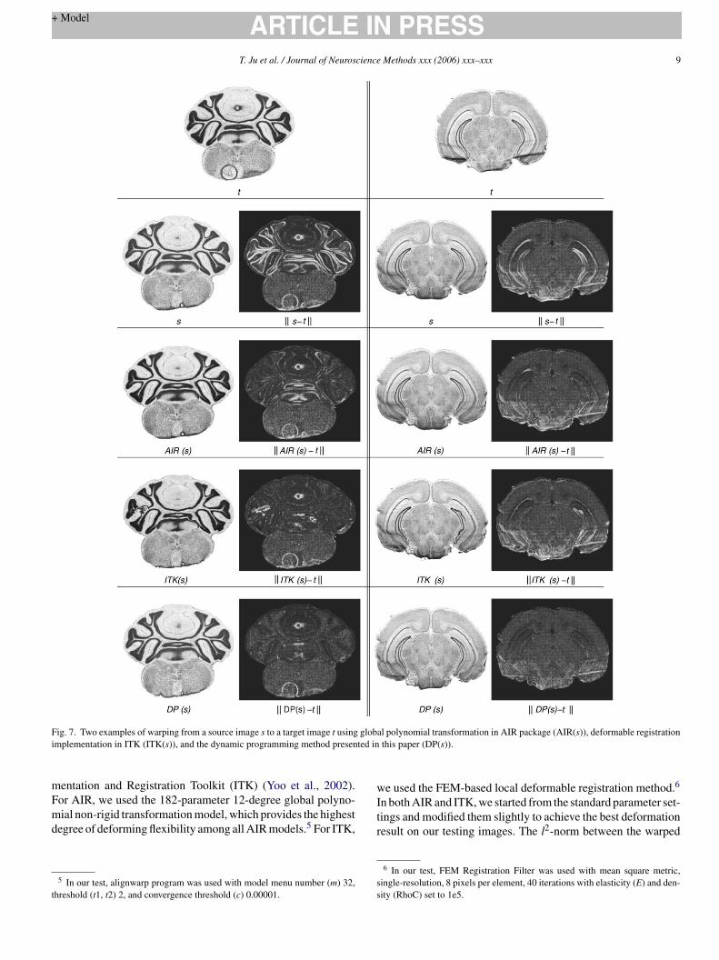
.2.4.3. Examples and comparison. Fig. 7 shows two examplesf warping adjacent Nissl-stained cryo-sections shown in Fig. 1.n each example, the goal is to find the warp that deforms theource section s to match the target section t. Sections are repre-ented as grayscale images of dimensions n = 850 and m = 670.e compare the result of applying our method4 to the result
f using two other popular warping methods: Automated Imageegistration (AIR) (Woods et al., 1998a), and NLM Insight Seg-
4 With elastic energy weights αX =αY = 0.00001, βX =βY = 0.02, γ = 0.005.
T. Ju et al. / Journal of Neuroscience Methods xxx (2006) xxx–xxx 9
Fig. 7. Two examples of warping from a source image s to a target image t using global polynomial transformation in AIR package (AIR(s)), deformable registrationimplementation in ITK (ITK(s)), and the dynamic programming method presented in this paper (DP(s)).
mentation and Registration Toolkit (ITK) (Yoo et al., 2002).For AIR, we used the 182-parameter 12-degree global polyno-mial non-rigid transformation model, which provides the highestdegree of deforming flexibility among all AIR models.5 For ITK,
5 In our test, alignwarp program was used with model menu number (m) 32,threshold (t1, t2) 2, and convergence threshold (c) 0.00001.
we used the FEM-based local deformable registration method.6
In both AIR and ITK, we started from the standard parameter set-tings and modified them slightly to achieve the best deformationresult on our testing images. The l2-norm between the warped
6 In our test, FEM Registration Filter was used with mean square metric,single-resolution, 8 pixels per element, 40 iterations with elasticity (E) and den-sity (RhoC) set to 1e5.
10 T. Ju et al. / Journal of Neuroscience Methods xxx (2006) xxx–xxx
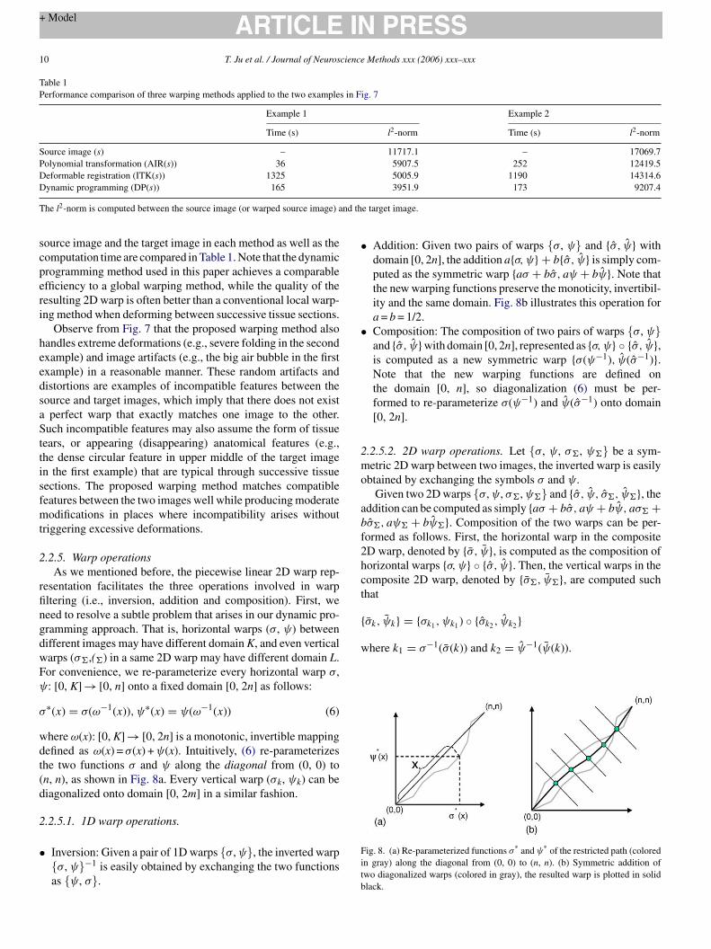
Table 1Performance comparison of three warping methods applied to the two examples in Fig. 7
Example 1 Example 2
Time (s) l2-norm Time (s) l2-norm
Source image (s) – 11717.1 – 17069.7Polynomial transformation (AIR(s)) 36 5907.5 252 12419.5Deformable registration (ITK(s)) 1325 5005.9 1190 14314.6Dynamic programming (DP(s)) 165 3951.9 173 9207.4
The l2-norm is computed between the source image (or warped source image) and the target image.
source image and the target image in each method as well as thecomputation time are compared in Table 1. Note that the dynamicprogramming method used in this paper achieves a comparableefficiency to a global warping method, while the quality of theresulting 2D warp is often better than a conventional local warp-ing method when deforming between successive tissue sections.
Observe from Fig. 7 that the proposed warping method alsohandles extreme deformations (e.g., severe folding in the secondexample) and image artifacts (e.g., the big air bubble in the firstexample) in a reasonable manner. These random artifacts anddistortions are examples of incompatible features between thesource and target images, which imply that there does not exista perfect warp that exactly matches one image to the other.Such incompatible features may also assume the form of tissuetears, or appearing (disappearing) anatomical features (e.g.,the dense circular feature in upper middle of the target imagein the first example) that are typical through successive tissuesections. The proposed warping method matches compatiblefeatures between the two images well while producing moderatemodifications in places where incompatibility arises withouttriggering excessive deformations.
2.2.5. Warp operationsAs we mentioned before, the piecewise linear 2D warp rep-
resentation facilitates the three operations involved in warpfiltering (i.e., inversion, addition and composition). First, wengdwFψ
σ
wdt(d
2
•
• Addition: Given two pairs of warps {σ, ψ} and {σ̂, ψ̂} withdomain [0, 2n], the addition a{σ,ψ} + b{σ̂, ψ̂} is simply com-puted as the symmetric warp {aσ + bσ̂, aψ + bψ̂}. Note thatthe new warping functions preserve the monoticity, invertibil-ity and the same domain. Fig. 8b illustrates this operation fora = b = 1/2.
• Composition: The composition of two pairs of warps {σ, ψ}and {σ̂, ψ̂}with domain [0, 2n], represented as {σ,ψ} ◦ {σ̂, ψ̂},is computed as a new symmetric warp {σ(ψ−1), ψ̂(σ̂−1)}.Note that the new warping functions are defined onthe domain [0, n], so diagonalization (6) must be per-formed to re-parameterize σ(ψ−1) and ψ̂(σ̂−1) onto domain[0, 2n].
2.2.5.2. 2D warp operations. Let {σ, ψ, σ�, ψ�} be a sym-metric 2D warp between two images, the inverted warp is easilyobtained by exchanging the symbols σ and ψ.
Given two 2D warps {σ,ψ, σ�,ψ�} and {σ̂, ψ̂, σ̂�, ψ̂�}, theaddition can be computed as simply {aσ + bσ̂, aψ + bψ̂, aσ� +bσ̂�, aψ� + bψ̂�}. Composition of the two warps can be per-formed as follows. First, the horizontal warp in the composite2D warp, denoted by {σ̄, ψ̄}, is computed as the composition ofhorizontal warps {σ,ψ} ◦ {σ̂, ψ̂}. Then, the vertical warps in thecomposite 2D warp, denoted by {σ̄�, ψ̄�}, are computed suchthat
{
w
Fitb
eed to resolve a subtle problem that arises in our dynamic pro-ramming approach. That is, horizontal warps (σ, ψ) betweenifferent images may have different domain K, and even verticalarps (σ�,(�) in a same 2D warp may have different domain L.or convenience, we re-parameterize every horizontal warp σ,: [0, K] → [0, n] onto a fixed domain [0, 2n] as follows:
∗(x) = σ(ω−1(x)), ψ∗(x) = ψ(ω−1(x)) (6)
here ω(x): [0, K] → [0, 2n] is a monotonic, invertible mappingefined as ω(x) = σ(x) +ψ(x). Intuitively, (6) re-parameterizeshe two functions σ and ψ along the diagonal from (0, 0) ton, n), as shown in Fig. 8a. Every vertical warp (σk, ψk) can beiagonalized onto domain [0, 2m] in a similar fashion.
.2.5.1. 1D warp operations.
Inversion: Given a pair of 1D warps {σ,ψ}, the inverted warp{σ, ψ}−1 is easily obtained by exchanging the two functionsas {ψ, σ}.
σ̄k, ψ̄k} = {σk1 , ψk1 ) ◦ {σ̂k2 , ψ̂k2}
here k1 = σ−1(σ̄(k)) and k2 = ψ̂−1(ψ̄(k)).
ig. 8. (a) Re-parameterized functions σ* and ψ* of the restricted path (coloredn gray) along the diagonal from (0, 0) to (n, n). (b) Symmetric addition ofwo diagonalized warps (colored in gray), the resulted warp is plotted in solidlack.
T. Ju et al. / Journal of Neuroscience Methods xxx (2006) xxx–xxx 11
3. Results
Here we report the validation methods and the correspondingresults for evaluating the effectiveness of the proposed recon-struction method both qualitatively (i.e., by visual examination)and quantitatively (i.e., by computing distance and smoothnessmeasures). These methods form a general framework for validat-ing any warp-based 3D reconstruction algorithm. The evaluationis carried out on two sets of data: a synthetic volume with knowndistortions, and real serial sections with unknown distortions. Allcomputations are performed on a commodity PC with 1.5 GHzAMD Athlon processor and 2.5 GB memory.
3.1. Using a synthetic volume
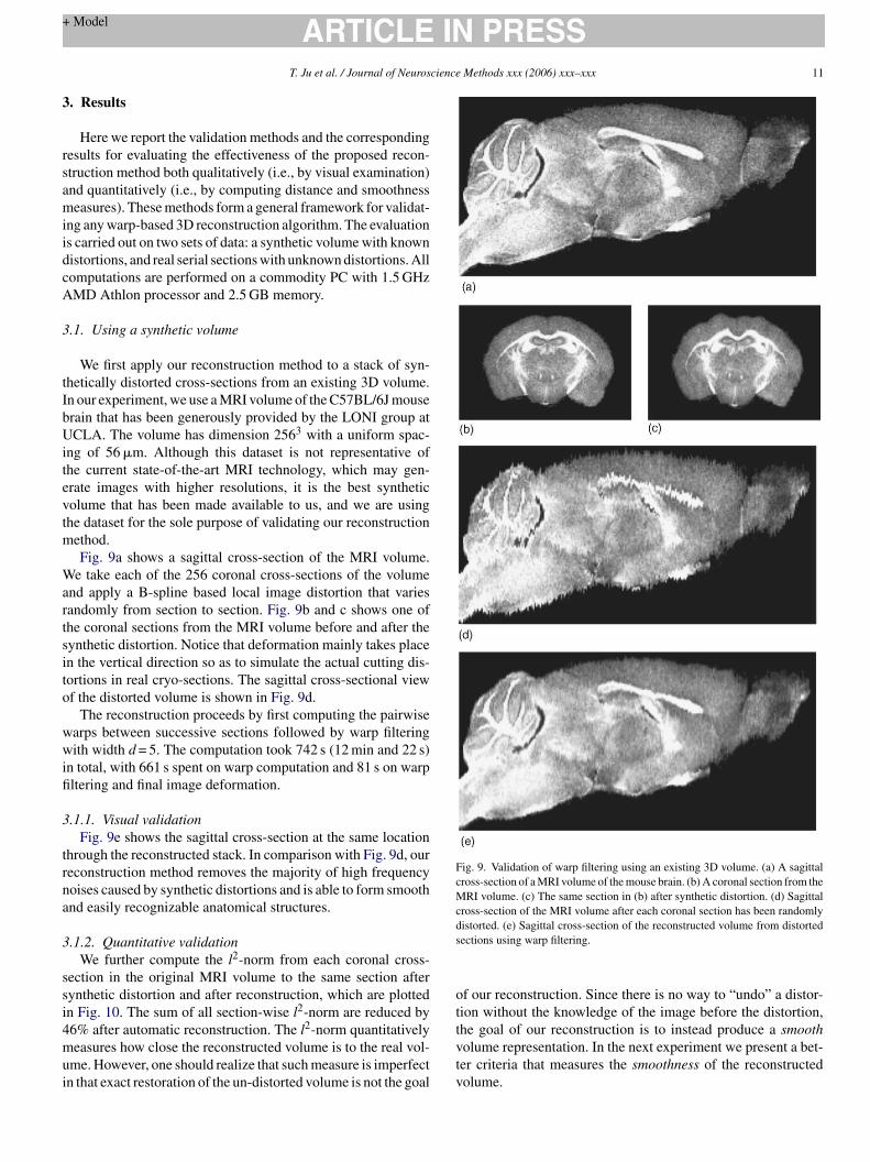
We first apply our reconstruction method to a stack of syn-thetically distorted cross-sections from an existing 3D volume.In our experiment, we use a MRI volume of the C57BL/6J mousebrain that has been generously provided by the LONI group atUCLA. The volume has dimension 2563 with a uniform spac-ing of 56 �m. Although this dataset is not representative ofthe current state-of-the-art MRI technology, which may gen-erate images with higher resolutions, it is the best syntheticvolume that has been made available to us, and we are usingthe dataset for the sole purpose of validating our reconstructionmethod.
Wartsito
wwifi
3
trna
3
ssi4mui
Fig. 9. Validation of warp filtering using an existing 3D volume. (a) A sagittalcross-section of a MRI volume of the mouse brain. (b) A coronal section from theMRI volume. (c) The same section in (b) after synthetic distortion. (d) Sagittalcross-section of the MRI volume after each coronal section has been randomlydistorted. (e) Sagittal cross-section of the reconstructed volume from distortedsections using warp filtering.
of our reconstruction. Since there is no way to “undo” a distor-tion without the knowledge of the image before the distortion,the goal of our reconstruction is to instead produce a smoothvolume representation. In the next experiment we present a bet-ter criteria that measures the smoothness of the reconstructedvolume.
Fig. 9a shows a sagittal cross-section of the MRI volume.e take each of the 256 coronal cross-sections of the volume
nd apply a B-spline based local image distortion that variesandomly from section to section. Fig. 9b and c shows one ofhe coronal sections from the MRI volume before and after theynthetic distortion. Notice that deformation mainly takes placen the vertical direction so as to simulate the actual cutting dis-ortions in real cryo-sections. The sagittal cross-sectional viewf the distorted volume is shown in Fig. 9d.
The reconstruction proceeds by first computing the pairwisearps between successive sections followed by warp filteringith width d = 5. The computation took 742 s (12 min and 22 s)
n total, with 661 s spent on warp computation and 81 s on warpltering and final image deformation.
.1.1. Visual validationFig. 9e shows the sagittal cross-section at the same location
hrough the reconstructed stack. In comparison with Fig. 9d, oureconstruction method removes the majority of high frequencyoises caused by synthetic distortions and is able to form smoothnd easily recognizable anatomical structures.
.1.2. Quantitative validationWe further compute the l2-norm from each coronal cross-
ection in the original MRI volume to the same section afterynthetic distortion and after reconstruction, which are plottedn Fig. 10. The sum of all section-wise l2-norm are reduced by6% after automatic reconstruction. The l2-norm quantitativelyeasures how close the reconstructed volume is to the real vol-
me. However, one should realize that such measure is imperfectn that exact restoration of the un-distorted volume is not the goal

12 T. Ju et al. / Journal of Neuroscience Methods xxx (2006) xxx–xxx
Fig. 10. The l2-norm from each of the 256 coronal sections of a MRI volume tothe same section after synthetic distortion (top curve) and to the reconstructedsection after warp filtering (bottom curve).
3.2. Using serial sections
We next test our method in reconstructing a 3D volumet-ric representation of the cell-density for the mouse brain fromserial sections. The input is a stack of 350 Nissl-stained imagesacquired by cyro-sectioning coronally a single frozen adultmouse brain (data preparation is detailed in Section 2.2.1). Eachimage is size 850 × 670 pixels at a resolution of 15 �m per pixel.
3.2.1. Pre-processingThe images were first registered using rigid-body transforma-
tions that align the symmetry axis of each coronal section to thevertical midline of the image and vertically adjust the sectionsusing reference sagittal histology sections from Paxino’s Atlas(Paxinos and Franklin, 2000). The axis alignment ensures thevertical direction of sectioning distortion, to which our warp-ing method is tailored. The vertical adjustment avoids causinga straight cylinder to be reconstructed as a sloping cylinder bywarp filtering. The resulting stack exhibits a natural 3D profilewith minimal translational and rotational differences betweenadjacent sections. Fig. 12 shows synthetic cross-section cuts inthe sagittal (a1) and horizontal (b1) direction through the rigid-body aligned stack.
Since the distance between adjacent sections (25 �m) farexceeds the size of a cell (∼10 �m), matching individual cellson two adjacent sections is not practical. To avoid aligningcfaiuat1bawwr
Fig. 11. A tissue section before (a) and after (b) applying the bilateral filter.
3.2.2. PerformanceThe computation of 349 pairwise warps between successive
sections consumes 27 MB memory and a total of 976 min (16 hand 16 min), averaging 168 s for each single warp. The perfor-mance of the subsequent warp filtering stage at different filteringwidth d is summarized in Table 2. We want to point out that sinceevery pairwise warp φk,k+1 is computed independently of eachother (and so is every filtered warp Φk), both warp computationand filtering can be greatly sped up by distributing the com-putation of different warps to different processors. Using thissimple parallelization scheme on a cluster of 16 processors, forexample, all pairwise warps would be computed within an hourwhile warp filtering would finish in approximately 10 min atd = 20.
3.2.3. Visual validation and comparisonFig. 12 shows cross-section cuts in the sagittal (a2) and hor-
izontal (b2) direction through the smooth volume reconstructedusing filtering width d = 20 (while the filtered warps are com-puted from bilaterally filtered images, they are applied to theoriginal images). Note that anatomical features become muchmore coherent in the reconstructed volume. The reconstructionalso recovers the shape of some key structures, such as the foldsin the cerebellum to the left and the hippocampus region in themiddle, whose profiles are barely recognizable or completelyi
uFtet
TCm
F
12
ellular details while matching macro features (e.g., the darkolds of the cerebellum) during warp computation, we firstpply a smoothing filter on the tissue sections before comput-ng the pairwise warps. Although a Gaussian filter could besed, an edge-preserving filter is more appropriate in that bound-ries between anatomical structures are retained. Fig. 11 showshe result of applying a bilateral filter (Tomasi and Manduchi,998) that we used in our experiment (other filters may alsoe used). Note that the filtered image exhibits clearer bound-ries between different anatomical features. After performingarp filtering on the bilaterally filtered images, the final warpsould then be applied to the original images for accurate
econstruction.
llegible in the original stack.For qualitative validation, we compare the reconstructed vol-
me to real histology sections from Paxino’s Atlas (Paxinos andranklin, 2000) at similar sagittal (a4) and horizontal (b4) loca-
ions. We find that the shapes of the anatomical structures recov-red in the reconstructed volume closely resemble the shapes ofhe corresponding structures in real tissue sections.
able 2omparison of performance for different filtering width d and the correspondingean and maximum smoothness measure Sk of the reconstructed volume
ilter width, d Time (min) Memory (MB) Mean Sk Maximum Sk
0a – – 85.43 1165.681 4.4 37 7.71 74.392 17.2 91 3.15 24.835 46.6 178 1.33 7.040 83.4 269 1.09 6.220 172.1 449 1.04 6.15
a Original stack.
T. Ju et al. / Journal of Neuroscience Methods xxx (2006) xxx–xxx 13
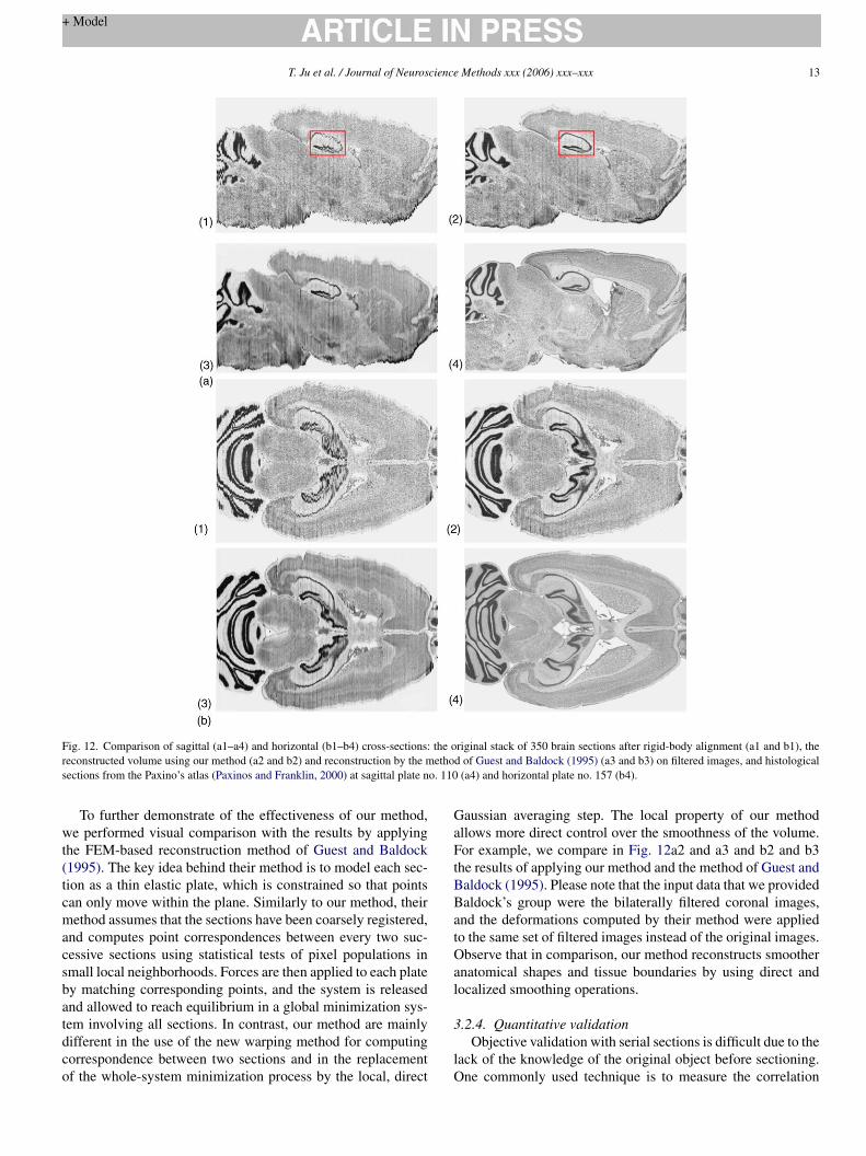
Fig. 12. Comparison of sagittal (a1–a4) and horizontal (b1–b4) cross-sections: the original stack of 350 brain sections after rigid-body alignment (a1 and b1), thereconstructed volume using our method (a2 and b2) and reconstruction by the method of Guest and Baldock (1995) (a3 and b3) on filtered images, and histologicalsections from the Paxino’s atlas (Paxinos and Franklin, 2000) at sagittal plate no. 110 (a4) and horizontal plate no. 157 (b4).
To further demonstrate of the effectiveness of our method,we performed visual comparison with the results by applyingthe FEM-based reconstruction method of Guest and Baldock(1995). The key idea behind their method is to model each sec-tion as a thin elastic plate, which is constrained so that pointscan only move within the plane. Similarly to our method, theirmethod assumes that the sections have been coarsely registered,and computes point correspondences between every two suc-cessive sections using statistical tests of pixel populations insmall local neighborhoods. Forces are then applied to each plateby matching corresponding points, and the system is releasedand allowed to reach equilibrium in a global minimization sys-tem involving all sections. In contrast, our method are mainlydifferent in the use of the new warping method for computingcorrespondence between two sections and in the replacementof the whole-system minimization process by the local, direct
Gaussian averaging step. The local property of our methodallows more direct control over the smoothness of the volume.For example, we compare in Fig. 12a2 and a3 and b2 and b3the results of applying our method and the method of Guest andBaldock (1995). Please note that the input data that we providedBaldock’s group were the bilaterally filtered coronal images,and the deformations computed by their method were appliedto the same set of filtered images instead of the original images.Observe that in comparison, our method reconstructs smootheranatomical shapes and tissue boundaries by using direct andlocalized smoothing operations.
3.2.4. Quantitative validationObjective validation with serial sections is difficult due to the
lack of the knowledge of the original object before sectioning.One commonly used technique is to measure the correlation
14 T. Ju et al. / Journal of Neuroscience Methods xxx (2006) xxx–xxx
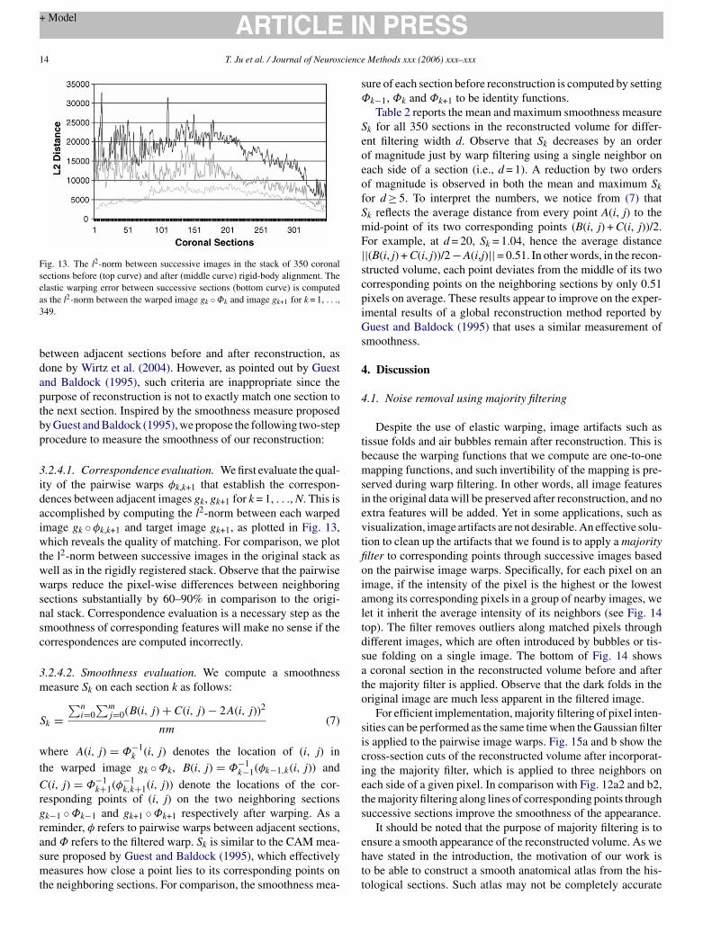
Fig. 13. The l2-norm between successive images in the stack of 350 coronalsections before (top curve) and after (middle curve) rigid-body alignment. Theelastic warping error between successive sections (bottom curve) is computedas the l2-norm between the warped image gk ◦Φk and image gk+1 for k = 1, . . .,349.
between adjacent sections before and after reconstruction, asdone by Wirtz et al. (2004). However, as pointed out by Guestand Baldock (1995), such criteria are inappropriate since thepurpose of reconstruction is not to exactly match one section tothe next section. Inspired by the smoothness measure proposedby Guest and Baldock (1995), we propose the following two-stepprocedure to measure the smoothness of our reconstruction:
3.2.4.1. Correspondence evaluation. We first evaluate the qual-ity of the pairwise warps φk,k+1 that establish the correspon-dences between adjacent images gk, gk+1 for k = 1, . . ., N. This isaccomplished by computing the l2-norm between each warpedimage gk ◦φk,k+1 and target image gk+1, as plotted in Fig. 13,which reveals the quality of matching. For comparison, we plotthe l2-norm between successive images in the original stack aswell as in the rigidly registered stack. Observe that the pairwisewarps reduce the pixel-wise differences between neighboringsections substantially by 60–90% in comparison to the origi-nal stack. Correspondence evaluation is a necessary step as thesmoothness of corresponding features will make no sense if thecorrespondences are computed incorrectly.
3.2.4.2. Smoothness evaluation. We compute a smoothnessmeasure Sk on each section k as follows:
S
∑n ∑m (B(i, j) + C(i, j) − 2A(i, j))2
wt
C
rgrasmt
sure of each section before reconstruction is computed by settingΦk−1, Φk and Φk+1 to be identity functions.
Table 2 reports the mean and maximum smoothness measureSk for all 350 sections in the reconstructed volume for differ-ent filtering width d. Observe that Sk decreases by an orderof magnitude just by warp filtering using a single neighbor oneach side of a section (i.e., d = 1). A reduction by two ordersof magnitude is observed in both the mean and maximum Skfor d ≥ 5. To interpret the numbers, we notice from (7) thatSk reflects the average distance from every point A(i, j) to themid-point of its two corresponding points (B(i, j) + C(i, j))/2.For example, at d = 20, Sk = 1.04, hence the average distance||(B(i, j) + C(i, j))/2 − A(i,j)|| = 0.51. In other words, in the recon-structed volume, each point deviates from the middle of its twocorresponding points on the neighboring sections by only 0.51pixels on average. These results appear to improve on the exper-imental results of a global reconstruction method reported byGuest and Baldock (1995) that uses a similar measurement ofsmoothness.
4. Discussion
4.1. Noise removal using majority filtering
Despite the use of elastic warping, image artifacts such astissue folds and air bubbles remain after reconstruction. This isbmsievtfioialtdsato
siciets
ehtt
k = i=0 j=0
nm(7)
here A(i, j) = Φ−1k (i, j) denotes the location of (i, j) in
he warped image gk ◦Φk, B(i, j) = Φ−1k−1(φk−1,k(i, j)) and
(i, j) = Φ−1k+1(φ−1
k,k+1(i, j)) denote the locations of the cor-esponding points of (i, j) on the two neighboring sectionsk−1 ◦Φk−1 and gk+1 ◦Φk+1 respectively after warping. As aeminder, φ refers to pairwise warps between adjacent sections,nd Φ refers to the filtered warp. Sk is similar to the CAM mea-ure proposed by Guest and Baldock (1995), which effectivelyeasures how close a point lies to its corresponding points on
he neighboring sections. For comparison, the smoothness mea-
ecause the warping functions that we compute are one-to-oneapping functions, and such invertibility of the mapping is pre-
erved during warp filtering. In other words, all image featuresn the original data will be preserved after reconstruction, and noxtra features will be added. Yet in some applications, such asisualization, image artifacts are not desirable. An effective solu-ion to clean up the artifacts that we found is to apply a majoritylter to corresponding points through successive images basedn the pairwise image warps. Specifically, for each pixel on anmage, if the intensity of the pixel is the highest or the lowestmong its corresponding pixels in a group of nearby images, weet it inherit the average intensity of its neighbors (see Fig. 14op). The filter removes outliers along matched pixels throughifferent images, which are often introduced by bubbles or tis-ue folding on a single image. The bottom of Fig. 14 showscoronal section in the reconstructed volume before and after
he majority filter is applied. Observe that the dark folds in theriginal image are much less apparent in the filtered image.
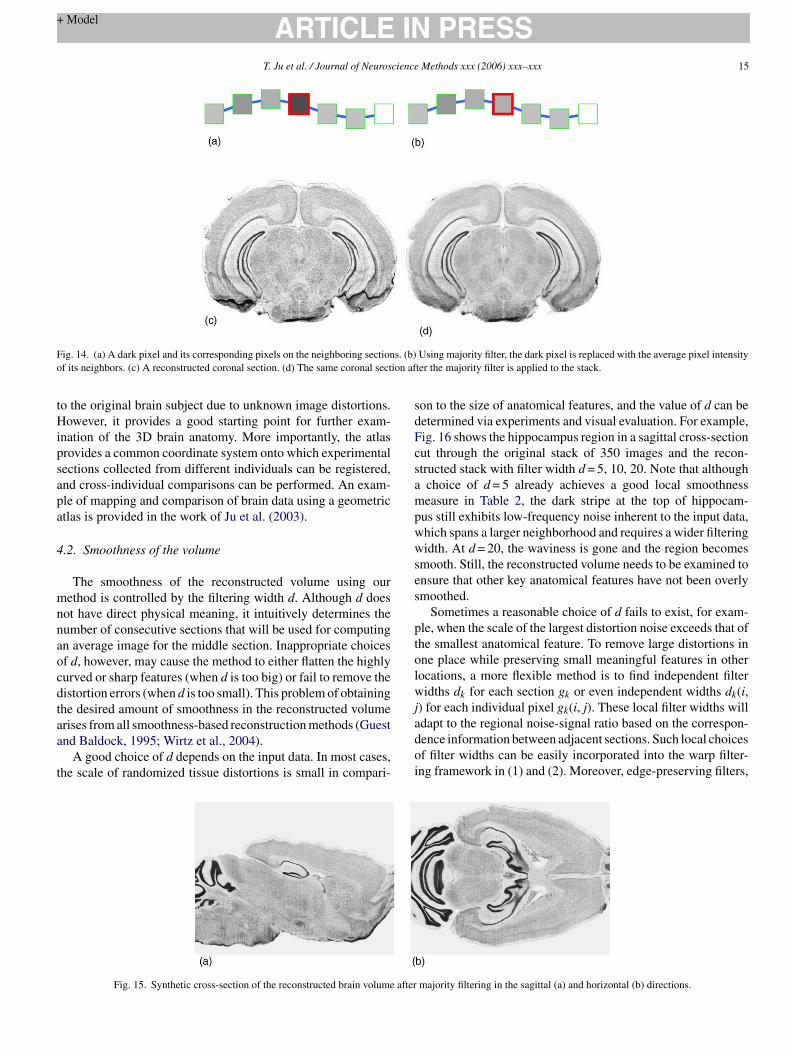
For efficient implementation, majority filtering of pixel inten-ities can be performed as the same time when the Gaussian filters applied to the pairwise image warps. Fig. 15a and b show theross-section cuts of the reconstructed volume after incorporat-ng the majority filter, which is applied to three neighbors onach side of a given pixel. In comparison with Fig. 12a2 and b2,he majority filtering along lines of corresponding points throughuccessive sections improve the smoothness of the appearance.
It should be noted that the purpose of majority filtering is tonsure a smooth appearance of the reconstructed volume. As weave stated in the introduction, the motivation of our work iso be able to construct a smooth anatomical atlas from the his-ological sections. Such atlas may not be completely accurate
T. Ju et al. / Journal of Neuroscience Methods xxx (2006) xxx–xxx 15
Fig. 14. (a) A dark pixel and its corresponding pixels on the neighboring sections. (b) Using majority filter, the dark pixel is replaced with the average pixel intensityof its neighbors. (c) A reconstructed coronal section. (d) The same coronal section after the majority filter is applied to the stack.
to the original brain subject due to unknown image distortions.However, it provides a good starting point for further exam-ination of the 3D brain anatomy. More importantly, the atlasprovides a common coordinate system onto which experimentalsections collected from different individuals can be registered,and cross-individual comparisons can be performed. An exam-ple of mapping and comparison of brain data using a geometricatlas is provided in the work of Ju et al. (2003).
4.2. Smoothness of the volume
The smoothness of the reconstructed volume using ourmethod is controlled by the filtering width d. Although d doesnot have direct physical meaning, it intuitively determines thenumber of consecutive sections that will be used for computingan average image for the middle section. Inappropriate choicesof d, however, may cause the method to either flatten the highlycurved or sharp features (when d is too big) or fail to remove thedistortion errors (when d is too small). This problem of obtainingthe desired amount of smoothness in the reconstructed volumearises from all smoothness-based reconstruction methods (Guestand Baldock, 1995; Wirtz et al., 2004).
A good choice of d depends on the input data. In most cases,the scale of randomized tissue distortions is small in compari-
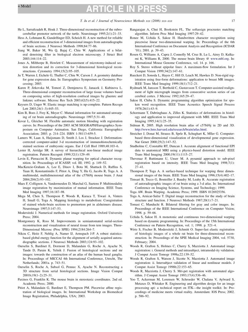
son to the size of anatomical features, and the value of d can bedetermined via experiments and visual evaluation. For example,Fig. 16 shows the hippocampus region in a sagittal cross-sectioncut through the original stack of 350 images and the recon-structed stack with filter width d = 5, 10, 20. Note that althougha choice of d = 5 already achieves a good local smoothnessmeasure in Table 2, the dark stripe at the top of hippocam-pus still exhibits low-frequency noise inherent to the input data,which spans a larger neighborhood and requires a wider filteringwidth. At d = 20, the waviness is gone and the region becomessmooth. Still, the reconstructed volume needs to be examined toensure that other key anatomical features have not been overlysmoothed.
Sometimes a reasonable choice of d fails to exist, for exam-ple, when the scale of the largest distortion noise exceeds that ofthe smallest anatomical feature. To remove large distortions inone place while preserving small meaningful features in otherlocations, a more flexible method is to find independent filterwidths dk for each section gk or even independent widths dk(i,j) for each individual pixel gk(i, j). These local filter widths willadapt to the regional noise-signal ratio based on the correspon-dence information between adjacent sections. Such local choicesof filter widths can be easily incorporated into the warp filter-ing framework in (1) and (2). Moreover, edge-preserving filters,
after
Fig. 15. Synthetic cross-section of the reconstructed brain volume majority filtering in the sagittal (a) and horizontal (b) directions.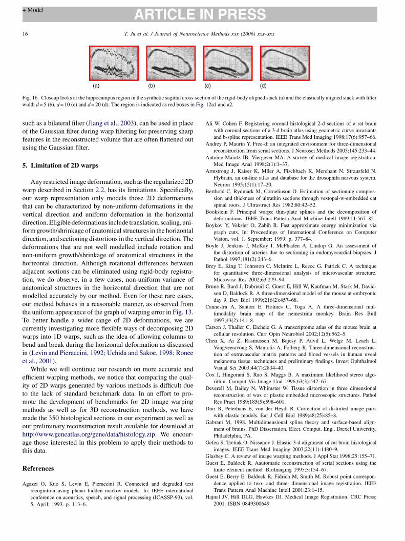
16 T. Ju et al. / Journal of Neuroscience Methods xxx (2006) xxx–xxx
Fig. 16. Closeup looks at the hippocampus region in the synthetic sagittal cross-section of the rigid-body aligned stack (a) and the elastically aligned stack with filterwidth d = 5 (b), d = 10 (c) and d = 20 (d). The region is indicated as red boxes in Fig. 12a1 and a2.
such as a bilateral filter (Jiang et al., 2003), can be used in placeof the Gaussian filter during warp filtering for preserving sharpfeatures in the reconstructed volume that are often flattened outusing the Gaussian filter.
5. Limitation of 2D warps
Any restricted image deformation, such as the regularized 2Dwarp described in Section 2.2, has its limitations. Specifically,our warp representation only models those 2D deformationsthat can be characterized by non-uniform deformations in thevertical direction and uniform deformation in the horizontaldirection. Eligible deformations include translation, scaling, uni-form growth/shrinkage of anatomical structures in the horizontaldirection, and sectioning distortions in the vertical direction. Thedeformations that are not well modelled include rotation andnon-uniform growth/shrinkage of anatomical structures in thehorizontal direction. Although rotational differences betweenadjacent sections can be eliminated using rigid-body registra-tion, we do observe, in a few cases, non-uniform variance ofanatomical structures in the horizontal direction that are notmodelled accurately by our method. Even for these rare cases,our method behaves in a reasonable manner, as observed fromthe uniform appearance of the graph of warping error in Fig. 13.To better handle a wider range of 2D deformations, we arecwbie
eitmmmohat
R
A
Ali W, Cohen F. Registering coronal histological 2-d sections of a rat brainwith coronal sections of a 3-d brain atlas using geometric curve invariantsand b-spline representation. IEEE Trans Med Imaging 1998;17(6):957–66.
Andrey P, Maurin Y. Free-d: an integrated environment for three-dimensionalreconstruction from serial sections. J Neurosci Methods 2005;145:233–44.
Antoine Maintz JB, Viergever MA. A survey of medical image registration.Med Image Anal 1998;2(1):1–37.
Armstrong J, Kaiser K, Mller A, Fischbach K, Merchant N, Strausfeld N.Flybrain, an on-line atlas and database for the drosophila nervous system.Neuron 1995;15(1):17–20.
Berthold C, Rydmark M, Corneliuson O. Estimation of sectioning compres-sion and thickness of ultrathin sections through vestopal-w-embedded catspinal roots. J Ultrastruct Res 1982;80:42–52.
Bookstein F. Principal warps: thin-plate splines and the decomposition ofdeformations. IEEE Trans Pattern Anal Machine Intell 1989;11:567–85.
Boykov Y, Veksler O, Zabih R. Fast approximate energy minimization viagraph cuts. In: Proceedings of International Conference on ComputerVision, vol. 1, September; 1999. p. 377–84.
Boyle J, Jenkins J, McKay I, McPhaden A, Lindop G. An assessment ofthe distortion of arteries due to sectioning in endomyocardial biopsies. JPathol 1997;181(2):243–6.
Brey E, King T, Johnston C, McIntire L, Reece G, Patrick C. A techniquefor quantitative three-dimensional analysis of microvascular structure.Microvasc Res 2002;63:279–94.
Brune R, Bard J, Dubreuil C, Guest E, Hill W, Kaufman M, Stark M, David-son D, Baldock R. A three-dimensional model of the mouse at embryonicday 9. Dev Biol 1999;216(2):457–68.
Cannestra A, Santori E, Holmes C, Toga A. A three-dimensional mul-timodality brain map of the nemestrina monkey. Brain Res Bull1997;43(2):141–8.
Carson J, Thaller C, Eichele G. A transcriptome atlas of the mouse brain at
C
C
D
D
G
G
GG
G
H
urrently investigating more flexible ways of decomposing 2Darps into 1D warps, such as the idea of allowing columns toend and break during the horizontal deformation as discussedn (Levin and Pieraccini, 1992; Uchida and Sakoe, 1998; Roneet al., 2001).
While we will continue our research on more accurate andfficient warping methods, we notice that comparing the qual-ty of 2D warps generated by various methods is difficult dueo the lack of standard benchmark data. In an effort to pro-
ote the development of benchmarks for 2D image warpingethods as well as for 3D reconstruction methods, we haveade the 350 histological sections in our experiment as well as
ur preliminary reconstruction result available for download atttp://www.geneatlas.org/gene/data/histology.zip. We encour-ge those interested in this problem to apply their methods tohis data.
eferences
gazzi O, Kuo S, Levin E, Pieraccini R. Connected and degraded textrecognition using planar hidden markov models. In: IEEE internationalconference on acoustics, speech, and signal processing (ICASSP-93), vol.5, April; 1993. p. 113–6.
cellular resolution. Curr Opin Neurobiol 2002;12(5):562–5.hen X, Ai Z, Rasmussen M, Bajcsy P, Auvil L, Welge M, Leach L,
Vangveeravong S, Maniotis A, Folberg R. Three-dimensional reconstruc-tion of extravascular matrix patterns and blood vessels in human uvealmelanoma tissue: techniques and preliminary findings. Invest OphthalmolVisual Sci 2003;44(7):2834–40.
ox I, Hingorani S, Rao S, Maggs B. A maximum likelihood stereo algo-rithm. Comput Vis Image Und 1996;63(3):542–67.
everell M, Bailey N, Whimster W. Tissue distortion in three dimensionalreconstruction of wax or plastic embedded microscopic structures. PatholRes Pract 1989;185(5):598–601.
urr R, Peterhans E, von der Heydt R. Correction of distorted image pairswith elastic models. Eur J Cell Biol 1989;48(25):85–8.
abrani M, 1998. Multidimensional spline theory and surface-based align-ment of brains. PhD Dissertation, Elect. Comput. Eng., Drexel University,Philadelphia, PA.
efen S, Tretiak O, Nissanov J. Elastic 3-d alignment of rat brain histologicalimages. IEEE Trans Med Imaging 2003;22(11):1480–9.
lasbey C. A review of image warping methods. J Appl Stat 1998;25:155–71.uest E, Baldock R. Aautomatic reconstruction of serial sections using the
finite element method. BioImaging 1995;3:154–67.uest E, Berry E, Baldock R, Fidrich M, Smith M. Robust point correspon-
dence applied to two- and three- dimensional image registration. IEEETrans Pattern Anal Machine Intell 2001;23:1–15.
ajnal JV, Hill DLG, Hawkes DJ. Medical Image Registration. CRC Press;2001. ISBN 0849300649.
T. Ju et al. / Journal of Neuroscience Methods xxx (2006) xxx–xxx 17
He L, Sarrafizadeh R, Houk J. Three-dimensional reconstruction of the rubro-cerebellar premotor network of the turtle. Neuroimage 1995;2(1):21–33.
Hess A, Lohmann K, Gundelfinger ED, Scheich H. A new method for reliableand efficient reconstruction of 3-dimensional images from autoradiographsof brain sections. J Neurosci Methods 1998;84:77–86.
Jiang W, Baker M, Wu Q, Bajaj C, Chiu W. Applications of a bilat-eral denoising filter in biological electron microscopy. J Struct Biol2003;144:114–22.
Jones A, Milthorpe B, Howlett C. Measurement of microtomy-induced sec-tion distortion and its correction for 3-dimensional histological recon-structions. Cytometry 1994;15(2):95–105.
Ju T, Warren J, Eichele G, Thaller C, Chiu W, Carson J. A geometry databasefor gene expression data. In: Eurographics Symposium on Geometry Pro-cessing; 2003.
Karen P, Jirkovska M, Tomori Z, Demjenova E, Janacek J, Kubinova L.Three-dimensional computer reconstruction of large tissue volumes basedon composing series of high-resolution confocal images by gluemrc andlinkmrc software. Microsc Res Tech 2003;62(5):415–22.
Keysers D, Unger W. Elastic image matching is np-complete. Pattern RecognLett 2003;24(1–3):445–53.
Kim B, Boes J, Frey K, Meyer C. Mutual information for automated unwarp-ing of rat brain autoradiographs. Neuroimage 1997;5:31–40.
Kovar L, Gleicher M. Flexible automatic motion blending with registrationcurves. In: Proceedings of the 2003 ACM SIGGRAPH/Eurographics Sym-posium on Computer Animation. San Diego, California: EurographicsAssociation; 2003. p. 214–224. ISBN 1-58113-659-5.
Lamers W, Laan A, Huijsmans D, Smith J, Los J, Strackee J. Deformation-corrected computer-aided 3-d reconstruction of immunohistochemicallystained sections of embryonic organs. Eur J Cell Biol 1989;48:103–6.
Lester H, Arridge SR. A survey of hierarchical non-linear medical imageregistration. Pattern Recognit 1999;32(1):129–49.
L
M
M
M
M
M
N
O
O
P
P
Rangarajan A, Chui H, Bookstein FL. The softassign procrustes matchingalgorithm. Inform Proc Med Imaging 1997:29–42.
Ronee M, Uchida S, Sakoe H. Handwritten character recognition usingpiecewise linear two-dimensional warping. In: Proceedings of the 6thInternational Conference on Document Analysis and Recognition (ICDAR’01); 2001. p. 39–43.
Rosen G, Williams A, Capra J, Connolly M, Cruz B, Lu L, Airey D, Kulka-rni K, Williams R, 2000. The mouse brain library @ www.mbl.org. In:International Mouse Genome Conference, vol. 14. p. 166.
Roy S. Stereo without epipolar lines: A maximum-flow formulation. Int JComput Vision 1999;34(2):147–61.
Rueckert D, Sonoda L, Hayes C, Hill D, Leach M, Hawkes D. Non-rigid reg-istration using free-form deformations: application to breast MR images.IEEE Trans Med Imaging 1999;18(1):712–21.
Rydmark M, Jansson T, Berthold C, Gustavsson T. Computer-assisted realign-ment of light micrograph images from consecutive section series of catcerebral cortex. J Microsc 1992;165:29–47.
Sakoe H, Chiba S. Dynamic programming algorithm optimization for spo-ken word recognition. IEEE Trans Acoustics Speech Signal Process1978;26(1):43–9.
Schormann T, Dabringhaus A, Zilles K. Statistics of deformations in histol-ogy and application to improved alignment with MRI. IEEE Trans MedImaging 1995;14(1):25–35.
Sidman R, 2005. High resolution brain atlas of c57bl/6j in 2D and 3D.http://www.hms.harvard.edu/research/brain/atlas.html.
Streicher J, Donat M, Strauss B, Sprle R, Schughart K, Mller G. Computer-based three-dimensional visualization of developmental gene expression.Nat Genet 2000;25(2):147–52.
Studholme C, Constable RT, Duncan J. Accurate alignment of functional EPIdata to anatomical MRI using a physics-based distortion model. IEEETrans Med Imaging 2000;19(11):1115–27.
T
T
T
TT
T
U
W
W
W
W
Y
evin E, Pieraccini R. Dynamic planar warping for optical character recog-nition. In: Proceedings of ICASSP, vol. III; 1992. p. 149–52.
acKenzie-Graham A, Lee E, Dinov I, Bota M, Shattuck D, Ruffins S,Yuan H, Konstantinidis F, Pitiot A, Ding Y, Hu G, Jacobs R, Toga A. Amultimodal, multidimensional atlas of the c57bl/6j mouse brain. J Anat2004;204(2):93–102.
aes F, Collignon A, Vandermeulen D, Marchal G, Suetens P. Multimodalityimage registration by maximization of mutual information. IEEE TransMed Imaging 1997;16:187–98.
ega M, Chen S, Thompson P, Woods R, Karaca T, Tiwari A, VintersH, Small G, Toga A. Mapping histology to metabolism: Coregistrationof stained whole-brain sections to premortem pet in alzheimers disease.Neuroimage 1997;5:147–53.
odersitzki J. Numerical methods for image registration. Oxford UniversityPress; 2004.
ontgomery K, Ross M. Improvements in semiautomated serial-sectionreconstruction and visualization of neural tissue from tem images. Three-Dimensional Microsc (Proc SPIE) 1994;2184:264–7.
ikou C, Heitz F, Nehlig A, Namer IJ, Armspach J-P. A robust statistics-based global energy function for the alignment of serially acquired autora-diographic sections. J Neurosci Methods 2003;124:93–102.
urselin S, Bardinet E, Dormont D, Malandain G, Roche A, Ayache N,Tande D, Parain K, Yelnik J. Fusion of histological sections and mrimages: towards the construction of an atlas of the human basal ganglia.In: Proceedings of MICCAI 4th International Conference, Utrecht, TheNetherlands; 2001a. p. 743–51.
urselin S, Roche A, Subsol G, Pennec X, Ayache N. Reconstructing a3D structure from serial histological sections. Image Vision Comput2001b;19(1–2):25–31.
axinos G, Franklin K. The mouse brain in stereotaxic coordinates. 2nd ed.Academic Press; 2000.
itiot A, Malandain G, Bardinet E, Thompson PM. Piecewise affine regis-tration of biological images. In: International Workshop on BiomedicalImage Registration, Philadelphia, USA; 2003.
hevenaz P, Ruttimann U, Unser M. A pyramid approach to sub-pixelregistration based on intensity. IEEE Trans Med Imaging 1998;7(1):27–41.
hompson P, Toga A. A surface-based technique for warping three dimen-sional images of the brain. IEEE Trans Med Imaging 1996;15(4):402–17.
imsari B, Tocco G, Bouteiller J, Baudry M, Leahy R. Accurate registrationof autoradiographic images of rat brain using a 3-d atlas. In: InternationalConference on Imaging Science, Systems, and Technology; 1999.
oga AW. Brain Warping. Academic Press; 1999. ISBN 0126925356.oga A, Arnicar-Sulze T. Digital image reconstruction for the study of brain
structure and function. J Neurosci Methods 1987;20(1):7–21.omasi C, Manduchi R. Bilateral filtering for gray and color images. In:
Proceedings of the IEEE International Conference on Computer Vision;1998. p. 59–66.
chida S, Sakoe H. A monotonic and continuous two-dimensional warpingbased on dynamic programming. In: Proceedings of the 15th InternationalConference on Pattern Recognition, vol. 1; 1998. p. 521–4.
irtz S, Fischer B, Modersitzki J, Schmitt O. Super-fast elastic registrationof histologic images of a whole rat brain for three-dimensional recon-struction. In: Proceedings of the SPIE Medical Imaging 2004, vol. 5730,February; 2004.
oods R, Grafton S, Holmes C, Cherry S, Mazziotta J. Automated imageregistration: i. General methods and intrasubject, intramodal-ity validation.J Comput Assist Tomogr 1998a;22:139–52.
oods R, Grafton S, Watson J, Sicotte N, Mazziotta J. Automated imageregistration: ii. Intersubject validation of linear and nonlinear models. JComput Assist Tomogr 1998b;22:153–65.
oods R, Mazziotta J, Cherry S. Mri-pet registration with automated algo-rithm. J Comput Assist Tomogr 1993;17(4):536–46.
oo T, Ackerman M, Lorensen W, Schroeder W, Chalana V, Aylward S,Metaxes D, Whitaker R. Engineering and algorithm design for an imageprocessing api: a technical report on ITK—the insight toolkit. In: Pro-ceedings of medicine meets virtual reality. Amsterdam: IOS Press; 2002.p. 586–92.