3d winding number: theory and application to medical … winding number: theory and application to...
TRANSCRIPT

3D winding number: theory and application to medicalimagingBecciu, A.; Fuster, A.; Pottek, M.; van den Heuvel, B.J.P.; ter Haar Romenij, B.M.; van Assen,H.C.Published in:International Journal of Biomedical Imaging
DOI:10.1155/2011/516942
Published: 01/01/2011
Document VersionPublisher’s PDF, also known as Version of Record (includes final page, issue and volume numbers)
Please check the document version of this publication:
• A submitted manuscript is the author's version of the article upon submission and before peer-review. There can be important differencesbetween the submitted version and the official published version of record. People interested in the research are advised to contact theauthor for the final version of the publication, or visit the DOI to the publisher's website.• The final author version and the galley proof are versions of the publication after peer review.• The final published version features the final layout of the paper including the volume, issue and page numbers.
Link to publication
Citation for published version (APA):Becciu, A., Fuster, A., Pottek, M., van den Heuvel, B. J. P., Haar Romenij, ter, B. M., & Assen, van, H. C. (2011).3D winding number: theory and application to medical imaging. International Journal of Biomedical Imaging,2011, 516942-1/13. [516942]. DOI: 10.1155/2011/516942
General rightsCopyright and moral rights for the publications made accessible in the public portal are retained by the authors and/or other copyright ownersand it is a condition of accessing publications that users recognise and abide by the legal requirements associated with these rights.
• Users may download and print one copy of any publication from the public portal for the purpose of private study or research. • You may not further distribute the material or use it for any profit-making activity or commercial gain • You may freely distribute the URL identifying the publication in the public portal ?
Take down policyIf you believe that this document breaches copyright please contact us providing details, and we will remove access to the work immediatelyand investigate your claim.
Download date: 07. Jun. 2018
Hindawi Publishing CorporationInternational Journal of Biomedical ImagingVolume 2011, Article ID 516942, 13 pagesdoi:10.1155/2011/516942
Research Article
3D Winding Number: Theory and Application to Medical Imaging
Alessandro Becciu,1 Andrea Fuster,1 Mark Pottek,2 Bart van den Heuvel,1
Bart ter Haar Romeny,1 and Hans van Assen1
1 Department of Biomedical Engineering, Eindhoven University of Technology, 5600 MB Eindhoven, The Netherlands2 Department of Biology, Kaiserslautern University of Technology, 67653 Kaiserslautern, Germany
Correspondence should be addressed to Andrea Fuster, [email protected]
Received 2 June 2010; Revised 20 September 2010; Accepted 1 November 2010
Academic Editor: Yangbo Ye
Copyright © 2011 Alessandro Becciu et al. This is an open access article distributed under the Creative Commons AttributionLicense, which permits unrestricted use, distribution, and reproduction in any medium, provided the original work is properlycited.
We develop a new formulation, mathematically elegant, to detect critical points of 3D scalar images. It is based on a topologicalnumber, which is the generalization to three dimensions of the 2D winding number. We illustrate our method by considering threedifferent biomedical applications, namely, detection and counting of ovarian follicles and neuronal cells and estimation of cardiacmotion from tagged MR images. Qualitative and quantitative evaluation emphasizes the reliability of the results.
1. Introduction
Critical points are very helpful for different purposes andapplications in computer vision as key points, landmarkpoints, anchor points, and others. In segmentation, forexample, critical points have been used to characterizedeforming areas of the brain [1] or to enhance ridges andvalleys in MR images [2]. In image matching, mappingsbetween the considered images are computed based ontheir critical points [3, 4]. Image matching has been alsoperformed through the so-called top points, critical points forwhich the determinant of the Hessian matrix is equal to zero[5, 6], or through the popular Harris points [7] and the SIFTkeypoint detector [8]. Critical points have also been used inmotion estimation algorithms, where the optic flow field isgenerated from a sparse set of velocities associated to multi-scale anchor points [9, 10].
Critical point detection is an established research field.Blom [11], for example, classifies critical points by count-ing the sign changes between the analyzed pixels and itsneighbors in a hexagonal grid. Nackman [12] defines theimage topology in terms of slope districts. The ridge andvalley lines are described as the ascending and descendingslopes coming from saddle points. The dales and hills areidentified as districts whose lines of slope converge to/come
from the same pit/peak. These methods have been extensivelyemployed for 2-dimensional applications. In recent years,there has been a strong increase of computational power, and3D scalar images are becoming the standard data of inves-tigation, especially in medical imaging. Three-dimensionalcritical point techniques allow for a more realistic analysisof human organ behavior. For example, tracking algorithmsapplied on a 2-dimensional heart image sequence retrieveonly in-plane contractions and rotations of the cardiac wallsbut miss the through-plane components. The through-planecomponents are instead retrieved with 3-dimensional opticflow approaches. In this paper, we show an application wherethe presented critical point detection algorithm is embeddedin a feature point-based motion estimation technique.
In this paper, we work with a topological number (fromhomotopy theory) that can locate critical points of scalarimages in an arbitrary number of dimensions. In two dimen-sions, it reduces to the so-called winding number and hasbeen studied in detail in [13–15]. In physics, and in moderncosmology in particular, the winding number appears in thecontext of topological defects such as monopoles, cosmicstrings, and domain walls (see, e.g., [16] and referencestherein). We consider this topological number in threedimensions and refer to it as 3D winding number. Propertiesof this approach are significant.
2 International Journal of Biomedical Imaging
(i) The 3D winding number provides information onthe character of the critical points.
(ii) The winding number is independent of the shape ofhypersurface S around which it is calculated. It is atopological entity.
The paper is organized in the following way. Aftersome preliminaries (Section 2.1), we treat extensively thetheoretical aspects of the winding number in three dimen-sions and explain the implementation of our algorithm(Sections 2.2 and 2.3). In Sections 2.4 and 2.5, we describea methodology to refine the position of the retrieved criticalpoints, and we propose a classification of critical points basedon the winding number. Furthermore, we test the viabilityof our method by considering three different biomedicalapplications, namely, follicle and neuronal cell counting andcardiac motion estimation in Sections 3.1, 3.2, and 3.3,respectively. Finally, in Section 4, we discuss the results andpossibilities for future work.
2. Theory
2.1. Preliminaries. A critical point of a smooth functionf (x1, . . . , xn) is a point x = (x1, . . . , xn) for which thegradient of f vanishes,∇ f |x = 0. In any other case, the pointis said to be regular. Critical points can be further classifieddepending on whether the Hessian matrix at the consideredpoint is singular:
det(∂i∂ j f )∣∣∣
x= 0. (1)
This is obviously the case if one or more matrix eigenvaluesare zero. Such critical points are called degenerate. Other-wise, we deal with nondegenerate critical points.
We are interested in finding and classifying critical pointsof a scalar image L(x). We will do so by computing atopological quantity ν at every point in the image. Thetopological number of a d-dimensional scalar image at apoint x (with at most isolated singularities) is defined by [13]
ν =∮
SΦ(x), (2)
where Φ is a (d − 1)-form depending on the image intensityand its derivatives (see, e.g., [17] for a general discussionof differential forms). The precise definition of Φ in ddimensions can be found in [13]. In this paper, we will onlyconsider the case d = 3 (further details are given in the nextsection). The integration is performed on a closed, oriented(hyper) surface S around the considered point.
An important property of Φ is the fact that it is a closedform, dΦ = 0. If the image has no singularities in the regionV enclosed by S, the generalized Stoke’s theorem can beapplied to (2):
ν =∮
SΦ(x) =
∫
VdΦ(x) ≡ 0. (3)
Therefore, the quantity ν is just zero at a regular point. Ata singular point, it takes values of kπ, with k some nonzero
integer number depending on the number of dimensions andthe character of the singularity. (This is true for d ≥ 2.)
The described number is called topological because itdoes not depend on the chosen hypersurface of integrationin (2). Another important property is the fact that it isconserved within such a hypersurface; that is, when two ormore singularities are enclosed, their topological numbersadd up. We refer to [13] for a more detailed discussion onthese and other properties of ν in an arbitrary number ofdimensions.
2.2. Winding Number in Three Dimensions. In three dimen-sions, the integrand in equation (2) is a 2-form given by [13]:
Φ = LidLj ∧ dLkεi jk
(LlLl)3/2 , i, j, k, l = x, y, z. (4)
Here, the indices i, j, k, l can take on values x, y, or z,L = L(x, y, z) is the intensity function of a 3-dimensionalimage, Lx,Ly ,Lz are the components of the spatial gradientof the intensity function, ∇L = (Lx,Ly ,Lz), and ε is the3-dimensional Levi-Civita symbol. The wedge product isrepresented by ∧. In this paper, we use Einstein’s summationconvention; that is, a sum is taken over repeated indicesappearing in both subscripts and superscripts. In explicitform, (4) reads
Φ = 2
‖∇L‖3
(
LxdLy ∧ dLz + LydLz ∧ dLx + LzdLx ∧ dLy
)
,
(5)
where ‖∇L‖ is the gradient norm. Using the followingrelations:
dLi = Lixdx + Liydy + Lizdz, (6)
we can rewrite (5) as
Φ = 2
‖∇L‖3
{
dx ∧ dy[(
LyxLzy − LyyLzx)
Lx
+(
LzxLxy − LzyLxx)
Ly
+(
LxxLyy − LxyLyx
)
Lz]
+ dy ∧ dz[(
LyyLzz − LyzLzy)
Lx
+(
LzyLxz − LzzLxy)
Ly
+(
LxyLyz − LxzLyy
)
Lz]
+ dz ∧ dx[(
LyzLzx − LyxLzz)
Lx
+(LzzLxx−LzxLxz)Ly
+(
LxzLyx−LxxLyz
)
Lz]}
.
(7)

International Journal of Biomedical Imaging 3
This expression was also given in [18]. After furtherinspection, we notice that it can be reformulated in thefollowing way:
Φ = 2
‖∇L‖3
{
dx ∧ dy[(
∇Lx ×∇Ly
)
· ∇L]
+ dy ∧ dz[(
∇Ly ×∇Lz)
· ∇L]
+dz ∧ dx[(∇Lz ×∇Lx) · ∇L]}
,
(8)
where ∇L = (Lx,Ly ,Lz) and
∇Lx ≡ ∂x(∇L) =(
Lxx ,Lyx,Lzx)
, (9)
∇Ly , ∇Lz are defined analogously. This new form is moreelegant and simpler to work with. Comparing (7) and (8) itis also clear that the latter form will be easier to implement.In what follows, we will therefore use expression (8) ratherthan (7). In compact form, we have
Φ = 1
‖∇L‖3
(
∇Li ×∇Lj
)
· ∇Ldxi ∧ dx j , (10)
where i, j take on values x, y, or z. In this formulation, it istrivial to check that Φ is antisymmetric as the vector productis anticommutative.
2.3. Implementation. We study the nature of every voxel byperforming the integration of expression (8) on a 3 × 3 ×3 cube that contains it. Note that, for each face of the cube,only one term in (8) survives in the integration given by (2).For example, if we integrate on a cube face with z = constant,it is clear that dz = 0, and therefore only the first term has tobe taken into account.
One of the issues we face in the implementation isthe integration of differential forms. We make use of thefollowing identity for integration of differential forms inEuclidean space [19]:
∫
Ωf(
x1, . . . , xn)
dx1 ∧ ·· · ∧ dxn
= ±∫
Ωf(
x1, . . . , xn)
dx1 · · · dxn.(11)
Here, f (x1, . . . , xn) dx1 ∧ · · · ∧ dxn is an n-form in Rn
and Ω is an oriented domain. (If the considered differentialform has more than one component the identity simplyholds for each one of them.) Note that the integral on theright-hand side is just the usual integral of the functionf (x1, . . . , xn). The sign on the right-hand side depends onthe orientation of the considered integration domain (+ forpositively oriented, − for negatively oriented). For example,
from (8) and (11), the integration on z = constant oppositecube faces reads
νxy =∫
z=const.Φ
= 2
‖∇L‖3
(∫
up
(
∇Lx ×∇Ly
)
· ∇Ldxdy
−∫
down
(
∇Lx ×∇Ly
)
· ∇Ldxdy)
.
(12)
We consider the image intensity function on the faces ofa 3 × 3 × 3 cube to be L = L(xα+a, yβ+b, zγ+c), where a,b, c are shifting indices of a plane on the cube taking onvalues 0, 1, 2 and α = 1, . . . ,NBx − 2, β = 1, . . . ,NBy − 2,γ = 1, . . . ,NBz − 2 are indices of the image volume withNBx, NBy, and NBz representing the volume size in x, y, andz directions. With these conventions, equation (12) can beexpressed numerically as
να,β,γxy =
2∑
a,b=0
(
∇Lx ×∇Ly
)
· ∇L(
xα+a, yβ+b, zγ+2
)
−2∑
a,b=0
(
∇Lx ×∇Ly
)
· ∇L(
xα+a, yβ+b, zγ)
.
(13)
The winding numbers on planes x = constant and y =constant can be computed in a similar way. The total windingnumber for the considered cube is then
να,β,γ = να,β,γxy + ν
α,β,γyz + ν
α,β,γzx . (14)
The numerical implementation of the 3D windingnumber algorithm can be summarized in the following steps.
(i) Load scalar image L(x, y, z).
(ii) Calculate the winding number for all voxels in theimage volume
for α = 1 to NBx − 2 dofor β = 1 to NBy − 2 do
for γ = 1 to NBz − 2 do
να,β,γ = να,β,γxy + ν
α,β,γyz + ν
α,β,γzx
end forend for
end for
(iii) Divide the outcomes of να,β,γ by 4π.
(iv) In order to distinguish the type of critical pointsretrieved (maxima or minima from saddles), extractthe sign of the Hessian matrix determinant at loca-tions, where να,β,γ /=0.
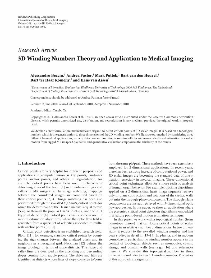
2.4. Refinement of Critical Point Positions. Due to signaldiscretization, the retrieved critical point location might notbe completely accurate (see Figure 1 for an illustration of thisissue for the 1D and 2D case). The position can be refined
4 International Journal of Biomedical Imaging
(a) (b)
Figure 1: Critical point refinement. (a) A continuum Gaussian signal in 1 dimension and the corresponding sampled signal. The sampledsignal shows maxima at two nearby positions (points in red), which are at different locations from the real maximum (point in green).(b) Rasterized version of a 2-dimensional Gaussian signal. Red points are the retrieved maxima, whereas the green point is the true maximumobtained after the refinement.
at subpixel level by considering the Taylor expansion of theintensity gradient around the retrieved point:
∇L(x) =(
Lx(xe) + (x− xe)Lxx(xe) +(
y − ye)
Lxy(xe)
+ (z − ze)Lxz(xe),
Ly(xe) + (x − xe)Lyx(xe) +(
y − ye)
Lyy(xe)
+ (z − ze)Lyz(xe),
Lz(xe) + (x− xe)Lzx(xe) +(
y − ye)
Lzy(xe)
+(z − ze)Lzz(xe))
,
(15)
where x = (x, y, z) and xe = (xe, ye, ze) denote the true andestimated critical point locations, respectively. We can writeequation (15) in a more compact form:
Li(x) = Li(xe) +(
j − je)
Li j(xe), (16)
where i, j can take on values x, y, or z. The intensity gradientat a critical point vanishes. The refined critical point positionis therefore
⎛
⎜⎜⎝
x
y
z
⎞
⎟⎟⎠=
⎛
⎜⎜⎝
xe
ye
ze
⎞
⎟⎟⎠−H−1(xe)
⎛
⎜⎜⎝
Lx(xe)
Ly(xe)
Lz(xe)
⎞
⎟⎟⎠. (17)
Here, H is the Hessian matrix. Equation (17) provides thecritical point position at subpixel level and can be iterateduntil the desired accuracy has been reached.
2.5. Classification of Critical Points. In three dimensions,there are four types of nondegenerate critical points, namely,minima, 1-saddles, 2-saddles, and maxima. They are charac-terized by the number of negative eigenvalues of the 3 × 3
Table 1: Index and winding number of critical points in 2D.
2D Index Winding number
Minimum 0 +2π
Saddle 1 −2π
Maximum 2 +2π
Hessian matrix, the index, at the corresponding point: 0, 1,2, or 3. Each 1-saddle (2-saddle) point is connected to two,not necessarily distinct, minima (maxima) by integral lines.A more detailed description of 3D saddle points can be foundin [20].
The winding number at a certain image point is givenby the integral of expression (10) on an appropriate surfaceenclosing the point. The winding number of (isolated)critical points in three dimensions takes values of 4 kπ, withk = ±1 [18, 21]. We will argue that the winding number canbe used for classification of extrema and saddle points in 3D.As a matter of fact, the winding number is able to distinguishbetween the two types of saddle points in 3D.
In Tables 1 and 2, we summarize the explicit values for theindex and winding number of the different types of criticalpoints. For completeness, we treat also the 2-dimensionalcase. Note that extrema in 3D can have either positive ornegative winding number, unlike the 2D case. Saddles havepositive or negative winding number as well, dependingon the type of saddle point. It is now possible to classifycritical points according to their winding number. Once thesign has been calculated, it suffices to examine the imageintensity at the considered point and its close neighborhoodto distinguish between a minimum and a 2-saddle or amaximum and a 1-saddle.
The proposed correspondence between the index andwinding number in three dimensions is well grounded.

International Journal of Biomedical Imaging 5
Table 2: Index and winding number of critical points in 3D.
3D Index Winding number
Minimum 0 +4π
1-saddle 1 −4π
2-saddle 2 +4π
Maximum 3 −4π
The following has been shown for a nondegenerate criticalpoint in an arbitrary number of dimensions [13]:
ν = sign(detH)Cd, (18)
where H is the Hessian matrix and Cd is a constantdepending only on the number of dimensions d. In threedimensions, Cd is equal to 4π. The relation between thewinding number and the sign of the Hessian in d = 3 is givenin Table 3. This is clearly in agreement with the postulatedwinding number for the different types of critical points.
3. Experiments
The proposed algorithm has been implemented in Math-ematica [22], and it has been tested on three differentbiomedical applications, namely, follicle detection, neuronalcell counting, and cardiac left ventricle motion analysis.In order to perform the experiments we make use of thescale-space framework [21, 23–26]. The Gaussian scale-spacerepresentation L : R3 × R+ of a 3-dimensional static imagex �→ f (x) ∈ L2(R3) is given by the spatial convolution with aGaussian kernel
L(x, s) = ( f ∗ φs)
(x) with φs(x) = 14πs
exp
(
−x2
4s
)
,
(19)
where x = (x, y, z) ∈ R3 and s > 0 represents the scale. In theremainder of the paper, the image intensity function shouldbe regarded as a function of both location and scale, L =L(x, s).
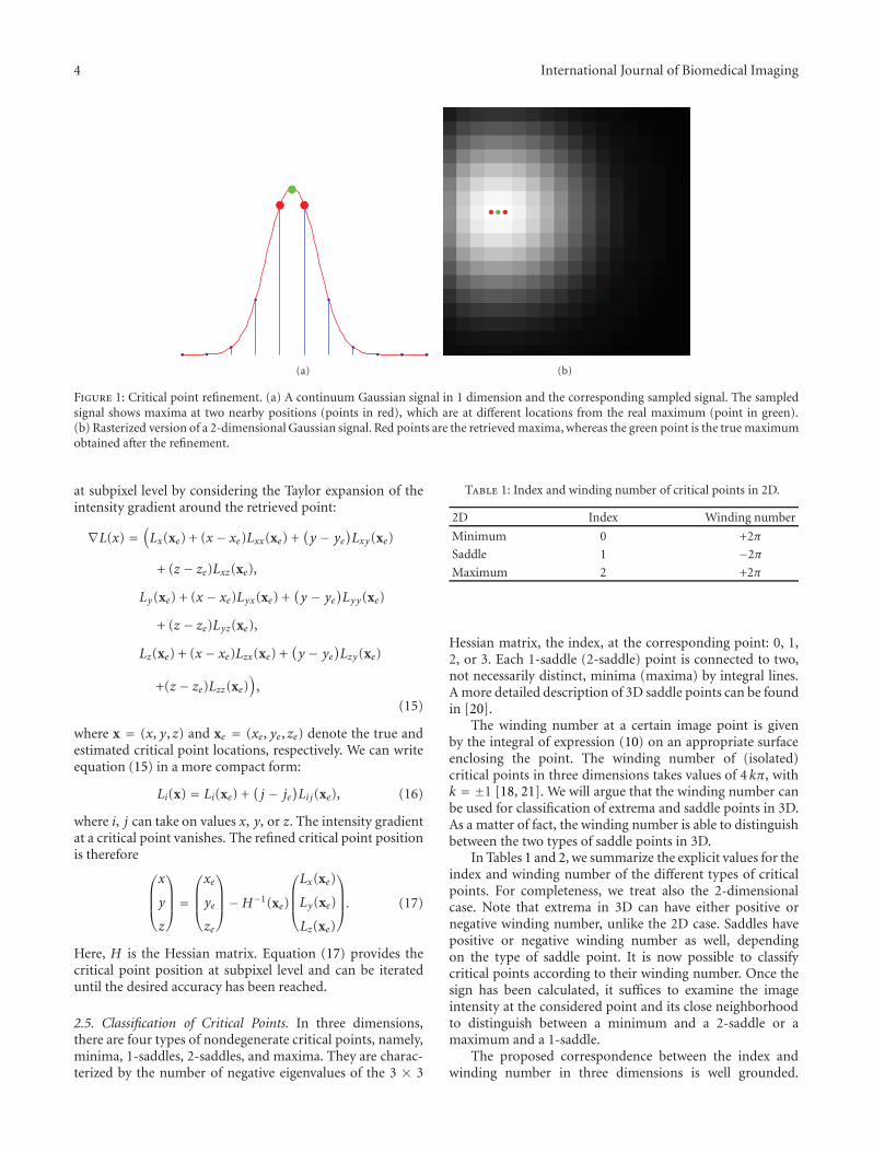
3.1. Follicle Detection. Ovarian follicles are the basic eggs ofthe female reproductive system. In particular, the numberof primordial follicles decreases with the age reaching aminimum during the menopause. Therefore, follicle analysisand counting may provide information on fertility prospects[27–29]. At the stage of development that they can bemeasured with 3D ultrasound, the human follicles presentroughly a spherical shape with a typical diameter of two tofive mm and appear darker with respect to surrounding tissueon ultrasound images (see Figures 2 and 3) [30].
Detection and counting of follicles is usually carried outmanually by inspecting the 2D slices from a 3D data set.This is a repetitive and tedious task which might introducemistakes especially in the typically noisy data sets. Robustand automated detection of follicles is therefore useful.
In the experiments, we automatically locate and countovarian follicles of three different patients using ultrasound
Table 3: Correspondence between the sign of the Hessian determi-nant and winding number for critical points in 3D.
3D Sign (detH) Winding number
Minimum + +4π
1-saddle − −4π
2-saddle + +4π
Maximum − −4π
image volumes with a size of 128 × 110 × 180, 138 ×116 × 176, and 180 × 108 × 126 voxels, respectively.Image acquisition has been carried out by an experiencedechographer with 3D ultrasound system Combison 5600(Kretz Technik AG, Medicor, Austria/Korea), which has beenequipped with a 12 MHz transvaginal 3D probe of 2.2 cm.The system performs image volume acquisition in about 2seconds and allows to reliably detect follicles with diameterof 3 mm or bigger. The image data were processed in order toinclude only the ovary after the scanning.
In the images, the center of the follicles exhibits a localminimum intensity. In these points, the intensity gradientvanishes. Due to the noisy nature of the images, the datasets exhibit several locations, where minima occur outsidethe follicle structure, producing false positives. The follicledetection algorithm consists of two main steps as follows.
(i) The 3D volume images were isotropically smoothedusing different scales.
(ii) Evaluation of the 3D winding number is carried outin order to retrieve the follicle centers.
In this procedure, we observe a tradeoff situation for thechoice of the proper scale. We notice that follicles presenta larger structure with respect to grains of the raw data. Inthe experiments, the scale is heuristically chosen sufficientlyhigh to avoid grain detection (see Figure 2(a), for criticalpoint detection at small scale), but not so high that smallerfollicles are missed. In this experiment, the results of folliclesextraction have been achieved at scale s = 9 voxels. The samecritical point detection procedure has been followed alsofor the experiments on neuronal cell counting and cardiacmotion estimation.
After critical point localization, the ovarian tissue hasbeen manually segmented in each slice in order to create amask and filter out the minima retrieved outside the ovarianboundaries (false positives) (see Figures 2(b) and 2(c)).
In the three data sets, results establish the presence of 19follicles for patient one, 8 for patient two, and 11 for patientthree. Manual counting of an expert revealed 17 follicles forpatient one, 7 for patient two, and 10 for patient 3 ([18, page68, Table 2, patient one, two, and three]). The computationaltime for each data set at scale s = 9 is less than 5 minuteson a PC with Intel Core 2 Duo 2 GHz processor and 4 GBRAM. The same computer has been used to carry outthe experiments of neuronal counting and cardiac motionestimation. For each individual, the amount of detectedfollicles indicates relatively good fertility prospects according
6 International Journal of Biomedical Imaging
(a) (b) (c)
Figure 2: Follicle detection. The red dots highlight the detected minima. (a) The image shows detected minima at scale s = 2. The image isvery noisy, and the algorithm detects also the minima corresponding to noisy grains (false positives). (b) The image shows minima detectedat scale s = 9. The arrow shows a minimum detected outside the ovarian tissue (false positive), whereas the red dot inside the ovarian tissuecorresponds to the center of a follicle. (c) In this image, the false positive outside the ovarian boundaries has been filtered out.
(a) (b)
(c) (d)
Figure 3: Follicle detection. 2D slices of the 3D ultrasound image smoothed data set corresponding to one of the patients. Lighter areasdisplay the ovary; dark circular blobs are the follicles. Red dots indicate retrieved local minima in 3D at scale s = 9 voxels.
to [31], especially in the case of patient one. In Figures 2 and3, retrieved minima are associated to red dots.
3.2. Neuronal Cell Counting in Cerebellum. The cerebellum isa region of the central nervous system located in the so-calledhindbrain. It is responsible for motor activity and regulationof muscle tone and also plays an important role in cognitiveand language functions in humans. In spite of occupyingonly around ten per cent of the whole brain volume, thecerebellum contains about fifty percent of all neurons. Thenumber of neurons varies depending on the age and healthcondition, such as in Alzheimer’s disease [32]. Cell densityis useful biomarker; however, neuronal cell counting is oftendone manually. This is a time-consuming task, where humanmistakes cannot be excluded. The eye of the observer willperform increasingly worse at such repetitive tasks. As aresult, estimations made for large number of cells may
become unreliable. For example, the number of Purkinjecells (the principal neurons of the cerebellum) in humanshas been estimated to be between 14 and 26 millions [33].Automatic counting methods are therefore preferable.
Several cell counting methods can be found in the liter-ature. They are mostly based on the cell density distributionin a certain volume and a good guess of the scientist [33–38]. These methods assume that the cell distribution in thevolume of reference stays uniform in the whole region ofinterest. If this is not the case, such methods will not providea reliable outcome. The algorithm proposed in this papercarries out automatic detection and counting without anyassumptions about the cell distribution. Therefore, it mayovercome the shortcomings of such techniques and providemore accurate results.
In the experiments, we consider two image volumes ofneurons labeled with propidium iodide with dimensions
International Journal of Biomedical Imaging 7
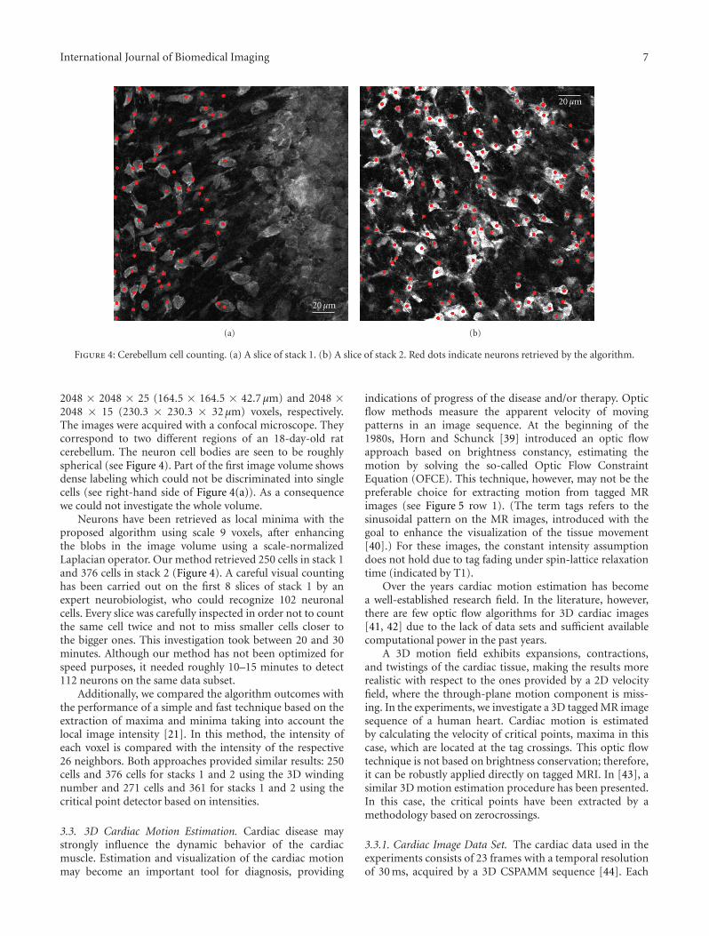
20 µm
(a)
20 µm
(b)
Figure 4: Cerebellum cell counting. (a) A slice of stack 1. (b) A slice of stack 2. Red dots indicate neurons retrieved by the algorithm.
2048 × 2048 × 25 (164.5 × 164.5 × 42.7 μm) and 2048 ×2048 × 15 (230.3 × 230.3 × 32 μm) voxels, respectively.The images were acquired with a confocal microscope. Theycorrespond to two different regions of an 18-day-old ratcerebellum. The neuron cell bodies are seen to be roughlyspherical (see Figure 4). Part of the first image volume showsdense labeling which could not be discriminated into singlecells (see right-hand side of Figure 4(a)). As a consequencewe could not investigate the whole volume.
Neurons have been retrieved as local minima with theproposed algorithm using scale 9 voxels, after enhancingthe blobs in the image volume using a scale-normalizedLaplacian operator. Our method retrieved 250 cells in stack 1and 376 cells in stack 2 (Figure 4). A careful visual countinghas been carried out on the first 8 slices of stack 1 by anexpert neurobiologist, who could recognize 102 neuronalcells. Every slice was carefully inspected in order not to countthe same cell twice and not to miss smaller cells closer tothe bigger ones. This investigation took between 20 and 30minutes. Although our method has not been optimized forspeed purposes, it needed roughly 10–15 minutes to detect112 neurons on the same data subset.
Additionally, we compared the algorithm outcomes withthe performance of a simple and fast technique based on theextraction of maxima and minima taking into account thelocal image intensity [21]. In this method, the intensity ofeach voxel is compared with the intensity of the respective26 neighbors. Both approaches provided similar results: 250cells and 376 cells for stacks 1 and 2 using the 3D windingnumber and 271 cells and 361 for stacks 1 and 2 using thecritical point detector based on intensities.
3.3. 3D Cardiac Motion Estimation. Cardiac disease maystrongly influence the dynamic behavior of the cardiacmuscle. Estimation and visualization of the cardiac motionmay become an important tool for diagnosis, providing
indications of progress of the disease and/or therapy. Opticflow methods measure the apparent velocity of movingpatterns in an image sequence. At the beginning of the1980s, Horn and Schunck [39] introduced an optic flowapproach based on brightness constancy, estimating themotion by solving the so-called Optic Flow ConstraintEquation (OFCE). This technique, however, may not be thepreferable choice for extracting motion from tagged MRimages (see Figure 5 row 1). (The term tags refers to thesinusoidal pattern on the MR images, introduced with thegoal to enhance the visualization of the tissue movement[40].) For these images, the constant intensity assumptiondoes not hold due to tag fading under spin-lattice relaxationtime (indicated by T1).
Over the years cardiac motion estimation has becomea well-established research field. In the literature, however,there are few optic flow algorithms for 3D cardiac images[41, 42] due to the lack of data sets and sufficient availablecomputational power in the past years.
A 3D motion field exhibits expansions, contractions,and twistings of the cardiac tissue, making the results morerealistic with respect to the ones provided by a 2D velocityfield, where the through-plane motion component is miss-ing. In the experiments, we investigate a 3D tagged MR imagesequence of a human heart. Cardiac motion is estimatedby calculating the velocity of critical points, maxima in thiscase, which are located at the tag crossings. This optic flowtechnique is not based on brightness conservation; therefore,it can be robustly applied directly on tagged MRI. In [43], asimilar 3D motion estimation procedure has been presented.In this case, the critical points have been extracted by amethodology based on zerocrossings.
3.3.1. Cardiac Image Data Set. The cardiac data used in theexperiments consists of 23 frames with a temporal resolutionof 30 ms, acquired by a 3D CSPAMM sequence [44]. Each
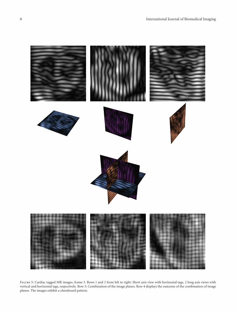
8 International Journal of Biomedical Imaging
Figure 5: Cardiac tagged MR images, frame 3. Rows 1 and 2 from left to right: Short axis view with horizontal tags, 2 long axis views withvertical and horizontal tags, respectively. Row 3: Combination of the image planes. Row 4 displays the outcome of the combination of imageplanes. The images exhibit a chessboard pattern.

International Journal of Biomedical Imaging 9
(a) (b) (c)
Figure 6: (a) The image shows a 2-dimensional slice of the 3-dimensional artificial phantom. (b) and (c) The images display the vector fieldof two successive frames of the phantom.
frame presents 14 slices in the short axis and two differentlong axis views (Figure 5 row 1); the images display a size of112 × 112 pixels, with 1 × 1 mm2 of pixel resolution. Therecorded slices are perpendicular with respect to each other,and, in the experiments, we combine them to obtain a grid(Figure 5 rows 2, 3, and 4, resp.). Due to sparseness in theslices, we interpolate the 14 slices in each frame in order toobtain image voxels of 112 × 112 × 112 pixels.
3.3.2. Calculation of Velocity at Critical Points Position. Asalready mentioned, we are interested in tracking the criticalpoints (maxima) that occur at the tag crossings of thechessboard-like pattern displayed in row 4 of Figure 5. In thiscase, we have a sequence of images, and therefore the imageintensity is also a function of time, that is, L(x(t), s, t), wherex(t) = (x(t), y(t), z(t)). The feature points move along with
the cardiac tissue, since they are part of the tags. We alsomentioned that MR tags fade due to relaxation time T1. Thisproperty does not influence the vanishing image gradient aslong as the tags are visible, and therefore it does not affect themaxima detection at the tag crossings.
By definition, the gradient of an image sequenceL(x(t), s, t) vanishes at critical point positions
∇L(x(t), s, t) = 0, (20)
where∇ denotes the spatial gradient and s and t represent thescale and time, respectively. In order to calculate the velocityat points with local maximum intensity (tag crossings) overtime, we differentiate (20) with respect to time t and applythe chain rule for implicit functions. Hence,
V(t) = d
dt
(
∇L(x(t), s, t)T)
=
⎛
⎜⎜⎝
Lxx(x(t), s, t)u(t) + Lxy(x(t), s, t)v(t) + Lxz(x(t), s, t)w(t) + Lxt(x(t), s, t)
Lyx(x(t), s, t)u(t) + Lyy(x(t), s, t)v(t) + Lyz(x(t), s, t)w(t) + Lyt(x(t), s, t)
Lzx(x(t), s, t)u(t) + Lzy(x(t), s, t)v(t) + Lzz(x(t), s, t)w(t) + Lzt(x(t), s, t)
⎞
⎟⎟⎠ = 0,
(21)
where d/dt is the total time derivative, T indicates transposeand u(t) = dx/dt, v(t) = dy/dt, and w(t) = dz/dt representthe velocity components in horizontal, vertical, and through-plane directions. In the experiments described in this section,we use a fixed scale s for all frames, for each experiment.Equation (21) can be reformulated in order to extract thevelocities u, v, and w. Hence,
V(t) =
⎛
⎜⎜⎝
u(t)
v(t)
w(t)
⎞
⎟⎟⎠= −H(x(t), s, t)−1
∂(
∇L(x(t), s, t)T)
∂t,
(22)
where H represents the spatial Hessian matrix of image L.In the literature, similar optic flow approaches that calculatevelocity estimation at feature point location using theHessian matrix are discussed in [9, 10, 43, 45].
3.3.3. Experiments on 3D Image Sequences. In order toassess the accuracy of the extracted vector field, the motionalgorithm has been tested on a sine phase grid artificialphantom (see Figure 6(a)) that exhibits contractions andexpansions (see vector fields in Figures 6(b) and 6(c)).The phantom consists of 19 frames with resolution of

10 International Journal of Biomedical Imaging
79 × 79 × 79 voxels and tags of 9 voxels wide. The groundtruth velocity vector of the phantom is given by
VGT(t) = (uGT, vGT,wGT)
= (m− 2n · t)(l + (m− n · t)t)
(
x− l, y − l, z − l)
,(23)
where x, y, z, t represent the spatial and temporal coordinatesand l, m, n are constant parameters (related to the length ofthe vectors) set to 40, 4, and 0.2, respectively.
The accuracy has been described in terms of averageangular error [46]:
AAE = arccos
⎛
⎝VGT(t)
√
uGT(t)2 + vGT(t)2 + wGT(t)2
· V(t)√
u(t)2 + v(t)2 + w(t)2
⎞
⎠.
(24)
The motion estimation of the artificial phantom has beencarried out from frame 8 to frame 11 in order to avoidoutliers due to temporal boundary conditions and at scales = 3.5 voxels. The computation of the optic flow field tookroughly 5 to 10 minutes per frame. The average angular erroris AAE = 2.68, degrees and the respective standard deviation(std) is std = 2.89 degrees.
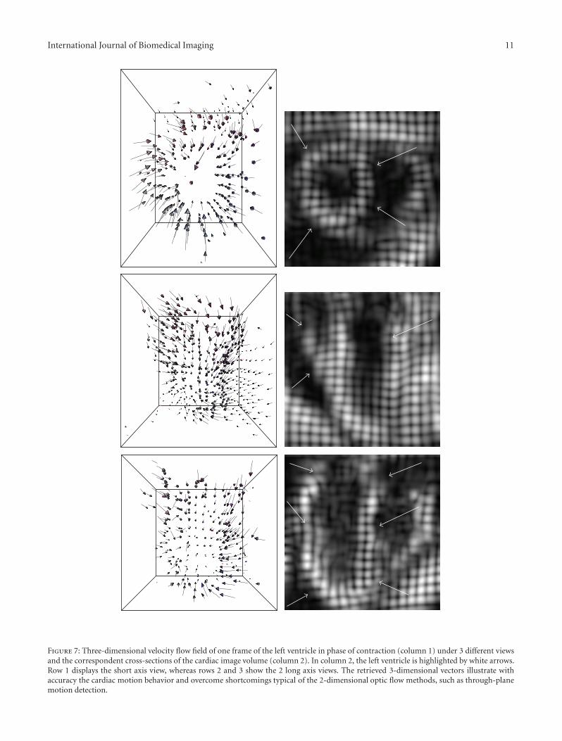
The optic flow algorithm has also been applied on areal sequence of 23 tagged volume MR images representinga human beating heart. The images exhibit a resolution of112 × 112 × 112 voxels and contained tags of 8 voxels wide.The velocity estimation is carried out at the tag crossings,the locations where critical points (maxima) are detected.The computation is carried out at a fixed scale of s = 3voxels and also took roughly 5 to 10 minutes per frame. InFigure 7, we show the retrieved motion field for the cardiacdata set investigated in the experiments. The images displaythe left ventricle in phase of contraction. After a qualitativeinspection, we notice that the algorithm retrieves a criticalpoint velocity in all three directions, providing valuableinformation for the quantitative analysis of the patient heart’sdynamic behavior.
4. Discussion and Conclusion
This paper investigates the 3D winding number as a effi-cient tool to retrieve and classify critical points in volumeimages. We provide a new formulation of the 3D windingnumber, simplifying the mathematics and implementationinvolved with respect to previous work [18]. We discuss theadvantages of the proposed technique such as its ability toboth locate and classify critical points. We carry out tests onthree different real applications (ovarian follicle and neuroncounting and cardiac motion estimation from tagged MRI).We finally discuss the experimental results, and we show theirqualitative and quantitative reliability.
In our applications, we highlight the usefulness ofour algorithm in tedious and repetitive operations such
as particle counting. The algorithm is able to find blobsand distinguish different cells located next to each otherin all data sets. In order to carry out manual counting,the user may either count cells slice by slice or, to speedup the procedure, may perform a 3D projection of theslices and carry out manual counting. In this latest case, hemay miss certain cells that are close but behind the oneslocated on the top. On the neuronal data set, for instance,our method detected 4 cells with roughly similar in-planelocation (distance less than 3.6 μm with respect to eachother) but different height.
In the experiment with the follicles and neurons, wehighlight that our algorithm detects a similar amountof follicles and neurons as a trained echographer andneurobiologist, which is already a strong advantage of theproposed method. However, critical point detection hasbeen carried out with a scale chosen globally. A criticalpoint extraction performed at small scale might detect noisygrains (false positives). On the other hand, a critical pointsearch carried out at too high scales may miss locationsof follicles/neurons that present a smaller structure withrespect to the other follicles/neurons in the data set. Theseproblems might be avoided by choosing different scales forfollicles/neurons with different sizes. In the future, we willcarry out experiments in this direction.
In the experiments, we assume that the cells have aroughly spherical shape. The neurons, however, have aroughly spherical head (the soma), connected to a tail (theaxon). In this case, extremal points were sometimes foundin the axons. The algorithm may, therefore, count twice thesame cell, increasing the error of the final estimation (seeFigure 4). A way to overcome this problem would be totake into account the geometry of the neuron and removeoutcomes coming from the axon. In future research, we willtune the algorithm to this specific application.
So far, we have considered the winding number in thecontext of scalar images. However, other applications of the3D winding number might be investigated such as detectionof singularities in 3D vector fields [47]. These have beenproved to be helpful in the visualization of 3D flow fields[48]. In the biomedical context, this could be applied toimprove the visualization of blood flow.
In the literature, as we already discussed, other criticalpoint retrieval methodologies are known. Critical pointsestimation can be carried out by taking into account thelocal intensity [21], where the intensity of each voxel iscompared with that of the respective 26 neighbors. InSection 3.2, we compared the performance of the 3D windingnumber algorithm with respect to that of the critical pointdetection method based on local intensity estimation. Bothmethods provided similar counting estimation. However,the intensity-based method is able to locate only maximaand minima, while the 3D winding number provides alsoinformation for saddle points. The 3D winding numberalgorithm is, therefore, preferable since it is able to charac-terize all types of critical points. In the future, we will carryout experiments on 3D saddle points detection, which haveinteresting applications in flow visualization [49, 50]. Finally,we will also compare the 3D winding number algorithm
International Journal of Biomedical Imaging 11
Figure 7: Three-dimensional velocity flow field of one frame of the left ventricle in phase of contraction (column 1) under 3 different viewsand the correspondent cross-sections of the cardiac image volume (column 2). In column 2, the left ventricle is highlighted by white arrows.Row 1 displays the short axis view, whereas rows 2 and 3 show the 2 long axis views. The retrieved 3-dimensional vectors illustrate withaccuracy the cardiac motion behavior and overcome shortcomings typical of the 2-dimensional optic flow methods, such as through-planemotion detection.
12 International Journal of Biomedical Imaging
with other feature points detectors such as SIFT for 3Dapplications.
Acknowledgments
The authors would like to thank Professor Sebastian Kozerkefor providing the 3D cardiac image data set, Ir. Roy van Peltfor bringing several relevant references to our attention, andIr. Vivian J. Roode for the development of the artificial phan-tom used in the optic flow application. The Stichting voor deTechnische Wetenschappen (STW) is also acknowledged forthe support on the ENN 06760 project. Andrea Fuster andAlessandro Becciu contributed equally to this paper.
References
[1] G. Wollny, M. Tittgemeyer, and F. Kruggel, “Segmentation ofvector fields by critical point analysis: application to braindeformation,” in Proceedings of International Conference onPattern Recognition, pp. 524–527, 2002.
[2] G. Fu, S. A. Hojjat, and A. C. F. Colchester, “Detection ofobjects by integrating watersheds and critical point analysis,”in Proceedings of the 6th International Conference on MedicalImage Computing and Computer-Assisted Intervention (MIC-CAI ’03), pp. 109–116, November 2003.
[3] Y. Shinagawa and T. L. Kunii, “Unconstrained automaticimage matching using multiresolutional critical-point filters,”IEEE Transactions on Pattern Analysis and Machine Intelligence,vol. 20, no. 9, pp. 994–1010, 1998.
[4] K. Habuka and Y. Shinagawa, “Image interpolation usingenhanced multiresolution critical-point filters,” InternationalJournal of Computer Vision, vol. 58, no. 1, pp. 19–35, 2004.
[5] B. Platel, E. Balmachnova, L. M. J. Florack, and B. M. teer HaarRomeny, “Top-points as interest points for image matching,”in Proceedings of the 9th European Conference on ComputerVision (ECCV ’06), vol. 3951 of Lecture Notes in ComputerScience, pp. 418–429, 2006.
[6] E. Balmachnova, L. M. J. Florack, B. Platel, F. M. W. Kanters,and B. M. ter Haar Romeny, “Stability of top-points in scalespace,” in Proceedings of the 5th International Conference onScale Space and PDE Methods in Computer Vision (Scale-Space’05), pp. 62–72, April 2005.
[7] C. Harris and M. Stephens, “A combined corner and edgedetector,” in Proceedings of the 4th Alvey Vision Conference, pp.147–151, 1988.
[8] D. G. Lowe, “Object recognition from local scale-invariant fea-tures,” in Proceedings of the 7th IEEE International Conferenceon Computer Vision (ICCV’99), pp. 1150–1157, September1999.
[9] P. van Dorst, B. Janssen, L. Florack, and B. M. ter HaarRomeny, “Optic flow using multi-scale anchor points,” inProceedings of the 13th International Conference on ComputerAnalysis of Images and Patterns (CAIP ’09), vol. 5702 of LectureNotes in Computer Science, pp. 1104–1112, Springer, 2009.
[10] A. Becciu, B. J. Janssen, H. van Assen, L. Florack, V. Roode, andB. M. ter Haar Romeny, “Extraction of cardiac motion usingscale-space features points and gauged reconstruction,” inProceedings of the 13th International Conference on ComputerAnalysis of Images and Patterns (CAIP ’09), vol. 5702 of LectureNotes in Computer Science, pp. 598–605, Springer, Munster,Germany, September 2009.
[11] J. Blom, Topological and geometrical aspects of image struc-ture, Ph.D. thesis, Department of Medical and PhysiologicalPhysics, University of Utrecht, 1992.
[12] L. R. Nackman, “Two-dimensional critical point configurationgraphs,” IEEE Transactions on Pattern Analysis and MachineIntelligence, vol. 6, no. 4, pp. 442–450, 1984.
[13] S. N. Kalitzin, B. M. ter Haar Romeny, A. H. Salden, P. F. M.Nacken, and M. A. Viergever, “Topological numbers and sin-gularities in scalar images: scale-space evolution properties,”Journal of Mathematical Imaging and Vision, vol. 9, no. 3, pp.253–269, 1998.
[14] S. N. Kalitzin, B. M. ter Haar Romeny, and M. A. Viergever,“On topological deep-structure segmentation,” in Proceedingsof the IEEE International Conference on Image Processing, S.Mitra, Ed., vol. 2, pp. 863–866, IEEE Computer Society Press,1997.
[15] S. N. Kalitzin, J. Staal, B. M. ter Haar Romeny, and M. A.Viergever, “A computational method for segmenting topo-logical point-sets and application to image analysis,” IEEETransactions on Pattern Analysis and Machine Intelligence, vol.23, no. 5, pp. 447–459, 2001.
[16] A. Vilenkin and E. P. S. Shellard, Cosmic Strings and OtherTopological Defects. Cambridge Monographs on MathematicalPhysics, Cambridge University Press, Cambridge, UK, 2000.
[17] M. Nakahara, Geometry, Topology and Physics, GraduateStudent Series in Physics, Taylor & Francis, London, UK, 2ndedition, 2003.
[18] B. M. ter Haar Romeny, B. Titulaer, S. N. Kalitzin etal., “Computer assisted human follicle analysis for fertilityprospects with 3D ultrasound,” in Information Processing inMedical Imaging, A. Kuba, M. Smal, and A. Todd-Pokropek,Eds., vol. 1613 of Lecture Notes in Computer Science, Springer,Heidelberg, Germany, 1999.
[19] T. Tao, “Differential forms and integration,” Tech. Rep.,Department of Mathematics, UCLA, 2007.
[20] Y. Matsumoto, Introduction to Morse Theory, American Math-ematical Society, Providence, RI, USA, 2001.
[21] B. M. ter Haar Romeny, Front-End Vision and Multi-ScaleImage Analysis: Multiscale Computer Vision Theory and Appli-cations, Written in Mathematica, Computational Imagingand Vision, Kluwer Academic Publishers, Dordrecht, TheNetherlands, 2003.
[22] Wolfram Research, http://www.wolfram.com/.[23] T. Iijima, “Basic theory on normalization of a pattern (in
case of typical one-dimensional pattern),” Bulletin of ElectricalLaboratory, vol. 26, pp. 368–388, 1962 (Japanese).
[24] T. Lindeberg, Scale-Space Theory in Computer Vision, TheKluwer International Series in Engineering and ComputerScience, Kluwer Academic Publishers, Dordrecht, The Nether-lands, 1994.
[25] J. J. Koenderink, “The structure of images,” Biological Cyber-netics, vol. 50, no. 5, pp. 363–370, 1984.
[26] L. M. J. Florack, Image Structure. Computational Imagingand Vision, Kluwer Academic Publishers, Dordrecht, TheNetherlands, 1997.
[27] M. Y. Chang, C. H. Chiang, T. H. Chiu, T. T. Hsieh, and Y. K.Soong, “The antral follicle count predicts the outcome of preg-nancy in a controlled ovarian hyperstimulation/intrauterineinsemination program,” Journal of Assisted Reproduction andGenetics, vol. 15, no. 1, pp. 12–17, 1998.
[28] M. J. Faddy, R. G. Gosden, A. Gougeon, S. J. Richardson, andJ. F. Nelson, “Accelerated disappearance of ovarian folliclesin mid-life: implications for forecasting menopause,” HumanReproduction, vol. 7, no. 10, pp. 1342–1346, 1992.

International Journal of Biomedical Imaging 13
[29] S. J. Richardson, V. Senikas, and J. F. Nelson, “Folliculardepletion during the menopausal transition: evidence foraccelerated loss and ultimate exhaustion,” Journal of ClinicalEndocrinology and Metabolism, vol. 65, no. 6, pp. 1231–1237,1987.
[30] E. A. McGee and A. J. W. Hsueh, “Initial and cyclic recruitmentof ovarian follicles,” Endocrine Reviews, vol. 21, no. 2, pp. 200–214, 2000.
[31] Advanced Fertility Center of Chicago, “Antral follicle counts,resting follicles, ovarian volume and ovarian reserve testingof egg supply and predicting response to ovarian stimulationdrugs,” http://www.advancedfertility.com/antralfollicles.htm.
[32] G. L. Wenk, “Neuropathologic changes in Alzheimer’s dis-ease,” Journal of Clinical Psychiatry, vol. 64, supplement 9, pp.7–10, 2003.
[33] L. Korbo and B. B. Andersen, “The distributions of Purkinjecell perikaryon and nuclear volume in human and ratcerebellum with the nucleator method,” Neuroscience, vol. 69,no. 1, pp. 151–158, 1995.
[34] L. Korbo, B. B. Andersen, O. Ladefoged, and A. Moller, “Totalnumbers of various cell types in rat cerebellar cortex estimatedusing an unbiased stereological method,” Brain Research, vol.609, no. 1-2, pp. 262–268, 1993.
[35] J. E. Axelrad, E. D. Louis, L. S. Honig et al., “Reduced Purkinjecell number in essential tremor: a postmortem study,” Archivesof Neurology, vol. 65, no. 1, pp. 101–107, 2008.
[36] O. F. Sonmez, E. Odaci, O. Bas, and S. Kaplan, “Purkinje cellnumber decreases in the adult female rat cerebellum followingexposure to 900 MHz electromagnetic field,” Brain Research,vol. 1356, no. C, pp. 95–101, 2010.
[37] L. Surchev, T. A. Nazwar, G. Weisheit, and K. Schilling,“Developmental increase of total cell numbers in the murinecerebellum,” Cerebellum, vol. 6, no. 4, pp. 315–320, 2007.
[38] E. R. Whitney, T. L. Kemper, M. L. Bauman, D. L. Rosene,and G. J. Blatt, “Cerebellar Purkinje cells are reduced in asubpopulation of autistic brains: a stereological experimentusing calbindin-D28k,” Cerebellum, vol. 7, no. 3, pp. 406–416,2008.
[39] B. K. P. Horn and B. G. Schunck, “Determining optical flow,”Artificial Intelligence, vol. 17, no. 1–3, pp. 185–203, 1981.
[40] E. A. Zerhouni, D. M. Parish, W. J. Rogers, A. Yang, and E.P. Shapiro, “Human heart: tagging with MR imaging—a newmethod for noninvasive assessment of myocardial motion,”Radiology, vol. 169, no. 1, pp. 59–63, 1988.
[41] J. L. Barron, “Experience with 3D optical flow on gated MRIcardiac datasets,” in Proceedings of the 1st Canadian Conferenceon Computer and Robot Vision, pp. 370–377, May 2004.
[42] L. Pan, J. L. Prince, J. A. C. Lima, and N. F. Osman,“Fast tracking of cardiac motion using 3D-HARP,” IEEETransactions on Biomedical Engineering, vol. 52, no. 8, pp.1425–1435, 2005.
[43] A. Becciu, H. van Assen, L. Florack, S. Kozerke, V. Roode,and B. M. ter Haar Romeny, “A multi-scale feature basedoptic flow method for 3D cardiac motion estimation,” inProceedings of the 2nd International Conference on Scale Spaceand Variational Methods in Computer Vision (SSVM ’09),vol. 5567 of Lecture Notes in Computer Science, pp. 588–599,Springer, Voss, Norway, June 2009.
[44] A. K. Rutz, S. Ryf, S. Plein, P. Boesiger, and S. Kozerke, “Accel-erated whole-heart 3D CSPAMM for myocardial motionquantification,” Magnetic Resonance in Medicine, vol. 59, no.4, pp. 755–763, 2008.
[45] B. J. Janssen, L. M. J. Florack, R. Duits, and B. M. ter HaarRomeny, “Optic flow from multi-scale dynamic anchor point
attributes,” in Proceedings of the 3rd International Conferenceon Image Analysis and Recognition (ICIAR ’06), vol. 4141 ofLecture Notes in Computer Science, pp. 767–779, 2006.
[46] J. L. Barron, D. J. Fleet, and S. S. Beauchemin, “Performanceof optical flow techniques,” International Journal of ComputerVision, vol. 12, no. 1, pp. 43–77, 1994.
[47] S. Mann and A. Rockwood, “Computing singularities of 3Dvector fields with geometric algebra,” in Proceedings of the IEEEVisualisation (VIS ’02), pp. 283–290, November 2002.
[48] R. S. Laramee, H. Hauser, L. Zhao, and F. H. Post, “Topology-cased flow visualization, the state of the art,” in Topology-BasedMethods in Visualization, pp. 1–19, Springer, Berlin, Germany,2007.
[49] H. Theisel, T. Weinkauf, H. C. Hege, and H. P. Seidel, “Sad-dle connectors—an approach to visualizing the topologicalskeleton of complex 3D vector fields,” in Proceedings of IEEEVisualization (VIS ’03), pp. 225–232, October 2003.
[50] F. Sadlo and R. Peikert, “Visualizing lagrangian coherentstructured and comparison to vector field topology,” inProceedings of the Workshop on Topology-Based Methods inVisualization, 2007.