3f3 4 basics of digital filters - fisika.ub.ac.id of... · 1 basics of digital filters elena...
TRANSCRIPT
1
Basics of Digital Filters
Elena Punskaya www-sigproc.eng.cam.ac.uk/~op205
Some material adapted from courses by Prof. Simon Godsill, Dr. Arnaud Doucet,
Dr. Malcolm Macleod and Prof. Peter Rayner
2
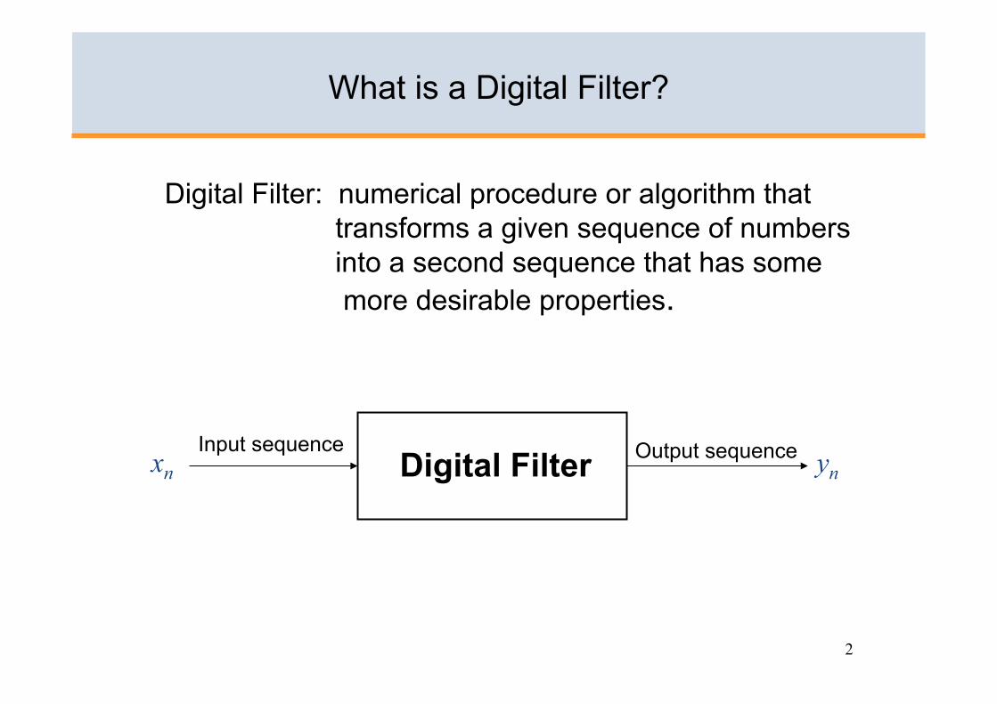
Digital Filter: numerical procedure or algorithm that transforms a given sequence of numbers into a second sequence that has some more desirable properties.
What is a Digital Filter?
Digital Filter Input sequence Output sequence xn yn
3
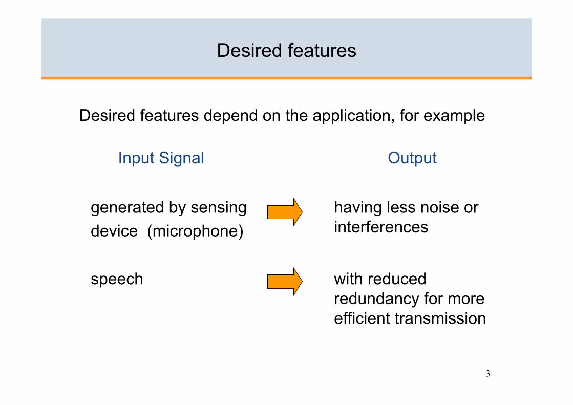
Desired features
Desired features depend on the application, for example
Input Signal Output
generated by sensing device (microphone)
having less noise or interferences
speech with reduced redundancy for more efficient transmission
4
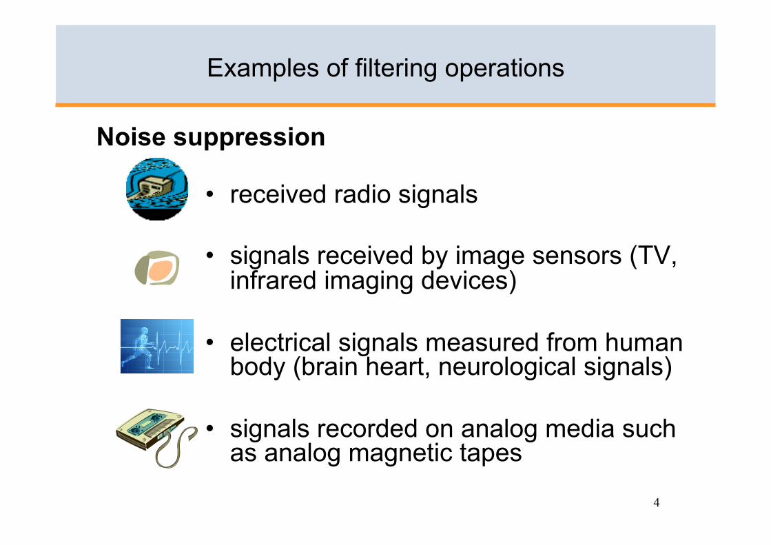
Examples of filtering operations
• received radio signals
• signals received by image sensors (TV, infrared imaging devices)
• electrical signals measured from human body (brain heart, neurological signals)
• signals recorded on analog media such as analog magnetic tapes
Noise suppression
5
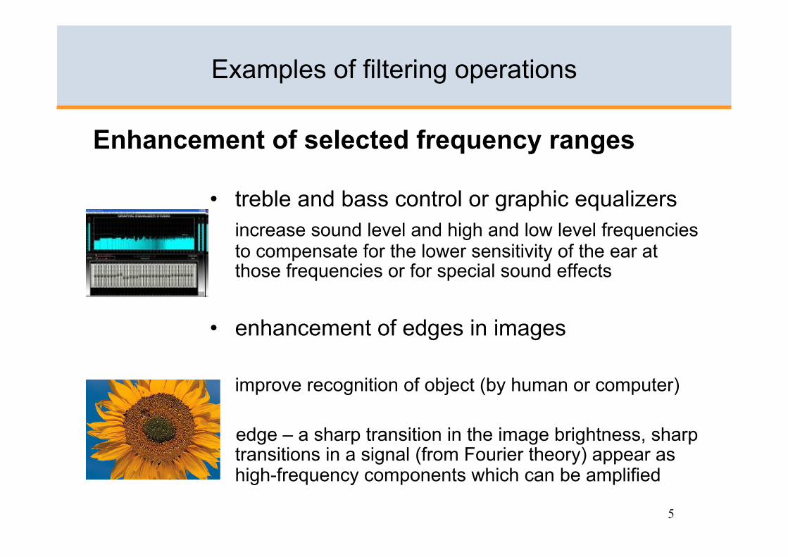
Examples of filtering operations
• treble and bass control or graphic equalizers increase sound level and high and low level frequencies to compensate for the lower sensitivity of the ear at those frequencies or for special sound effects
• enhancement of edges in images
improve recognition of object (by human or computer)
edge – a sharp transition in the image brightness, sharp transitions in a signal (from Fourier theory) appear as high-frequency components which can be amplified
Enhancement of selected frequency ranges
6
Examples of filtering operations
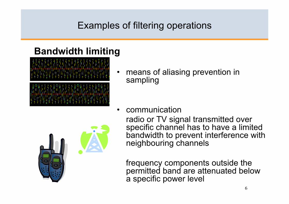
• means of aliasing prevention in sampling
• communication radio or TV signal transmitted over
specific channel has to have a limited bandwidth to prevent interference with neighbouring channels
frequency components outside the permitted band are attenuated below a specific power level
Bandwidth limiting

7
• differentiation • integration • Hilbert transform
Specific operations
Examples of filtering operations
These operations can be approximated by digital filters operating on the sampled input signal
8
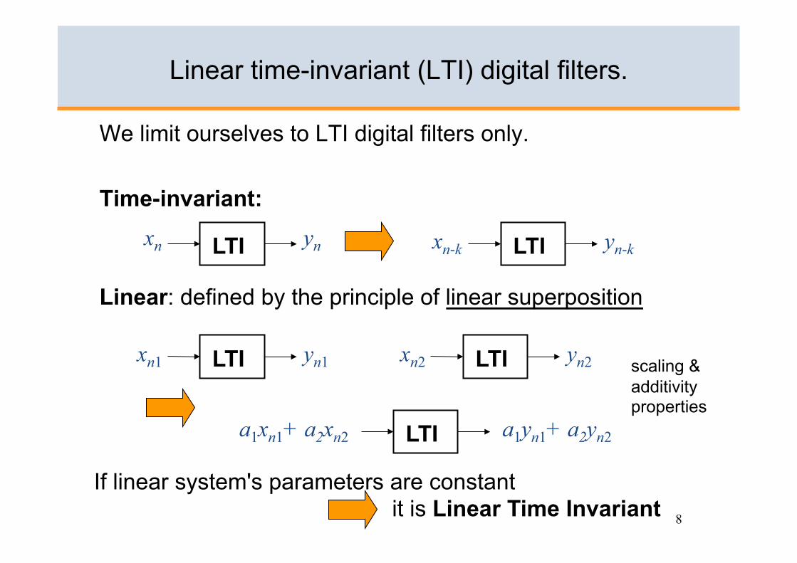
Linear time-invariant (LTI) digital filters.
We limit ourselves to LTI digital filters only.
Time-invariant:
Linear: defined by the principle of linear superposition
LTI xn1 yn1 LTI xn2 yn2
LTI a1xn1+ a2xn2 a1yn1+ a2yn2
scaling & additivity properties
LTI LTI xn-k yn-k
If linear system's parameters are constant it is Linear Time Invariant
xn yn
9
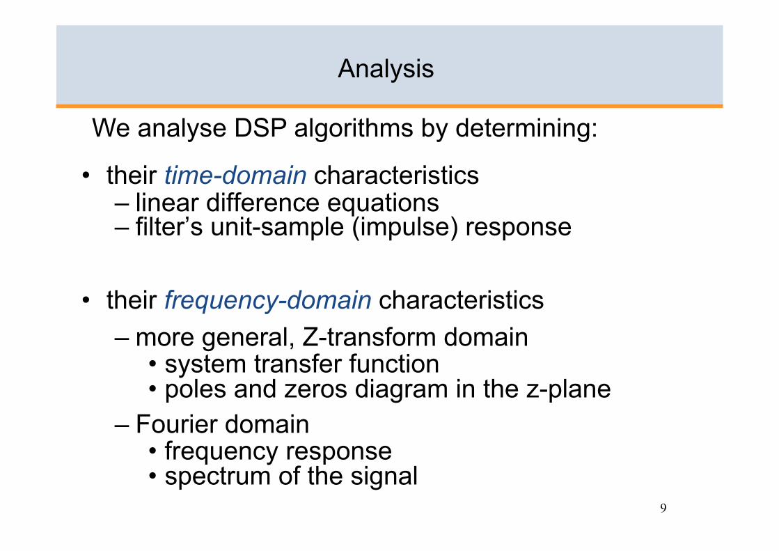
Analysis
• their time-domain characteristics – linear difference equations – filter’s unit-sample (impulse) response
• their frequency-domain characteristics – more general, Z-transform domain
• system transfer function • poles and zeros diagram in the z-plane
– Fourier domain • frequency response • spectrum of the signal
We analyse DSP algorithms by determining:
10
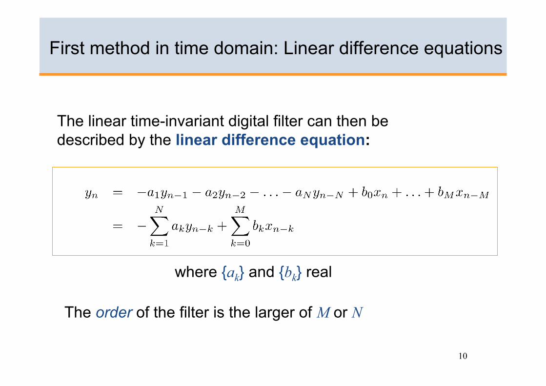
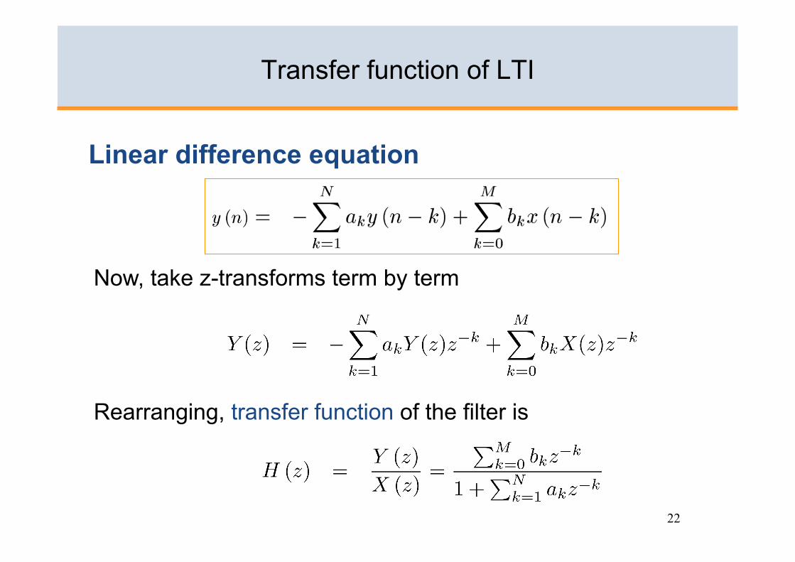
First method in time domain: Linear difference equations
The linear time-invariant digital filter can then be described by the linear difference equation:
where {ak} and {bk} real
The order of the filter is the larger of M or N
11
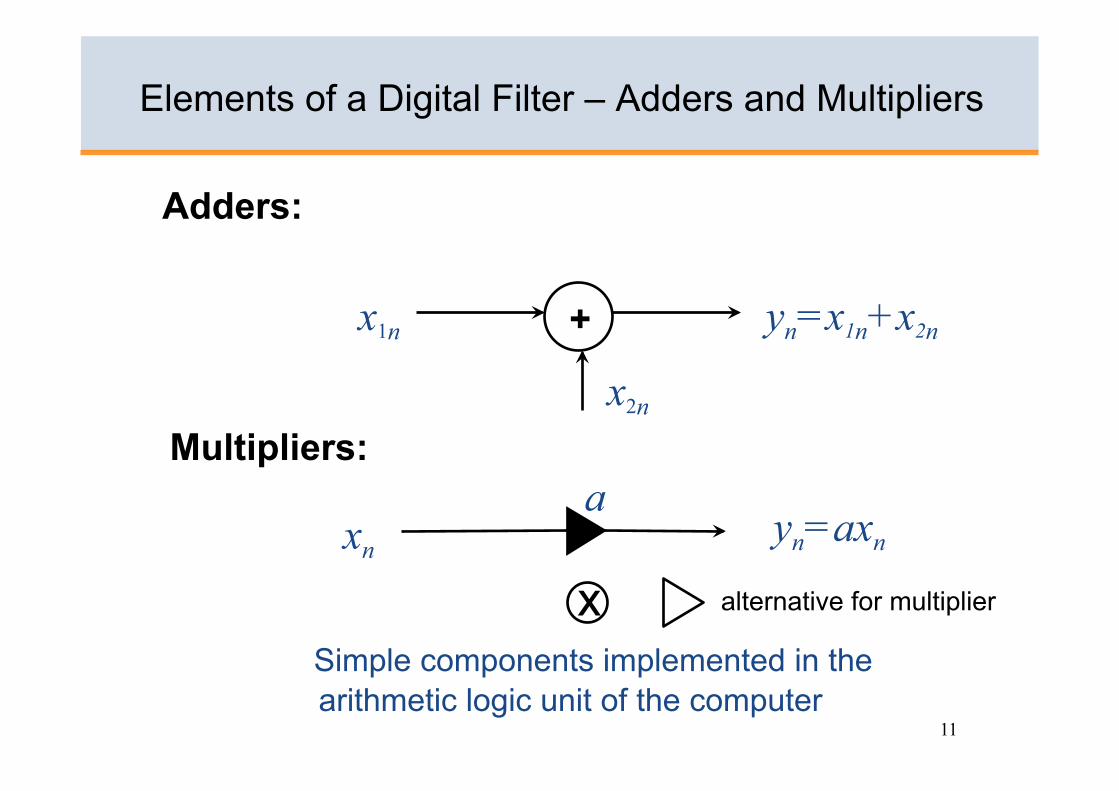
Elements of a Digital Filter – Adders and Multipliers
Adders:
Multipliers:
Simple components implemented in the arithmetic logic unit of the computer
x2n
+ x1n yn=x1n+x2n
xn yn=axn
a
alternative for multiplier x
12
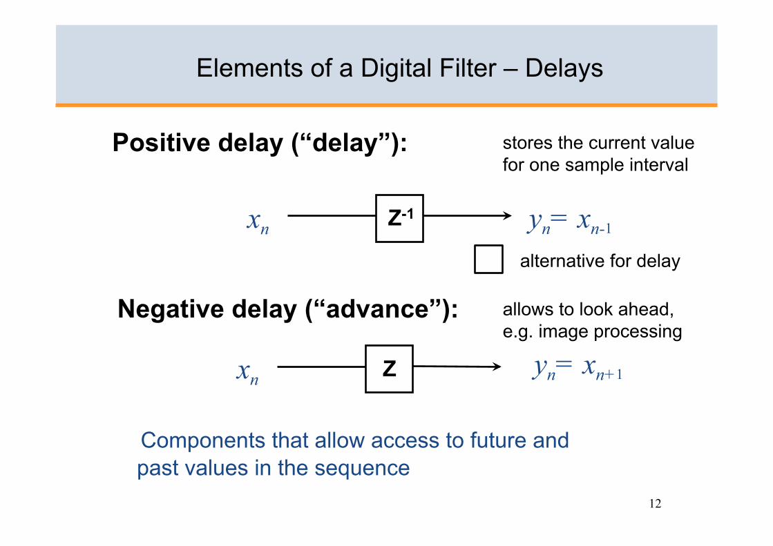
Elements of a Digital Filter – Delays
Positive delay (“delay”):
Negative delay (“advance”):
Components that allow access to future and past values in the sequence
yn= xn-1
yn= xn+1
Z-1 xn
xn Z
stores the current value for one sample interval
allows to look ahead, e.g. image processing
alternative for delay
13
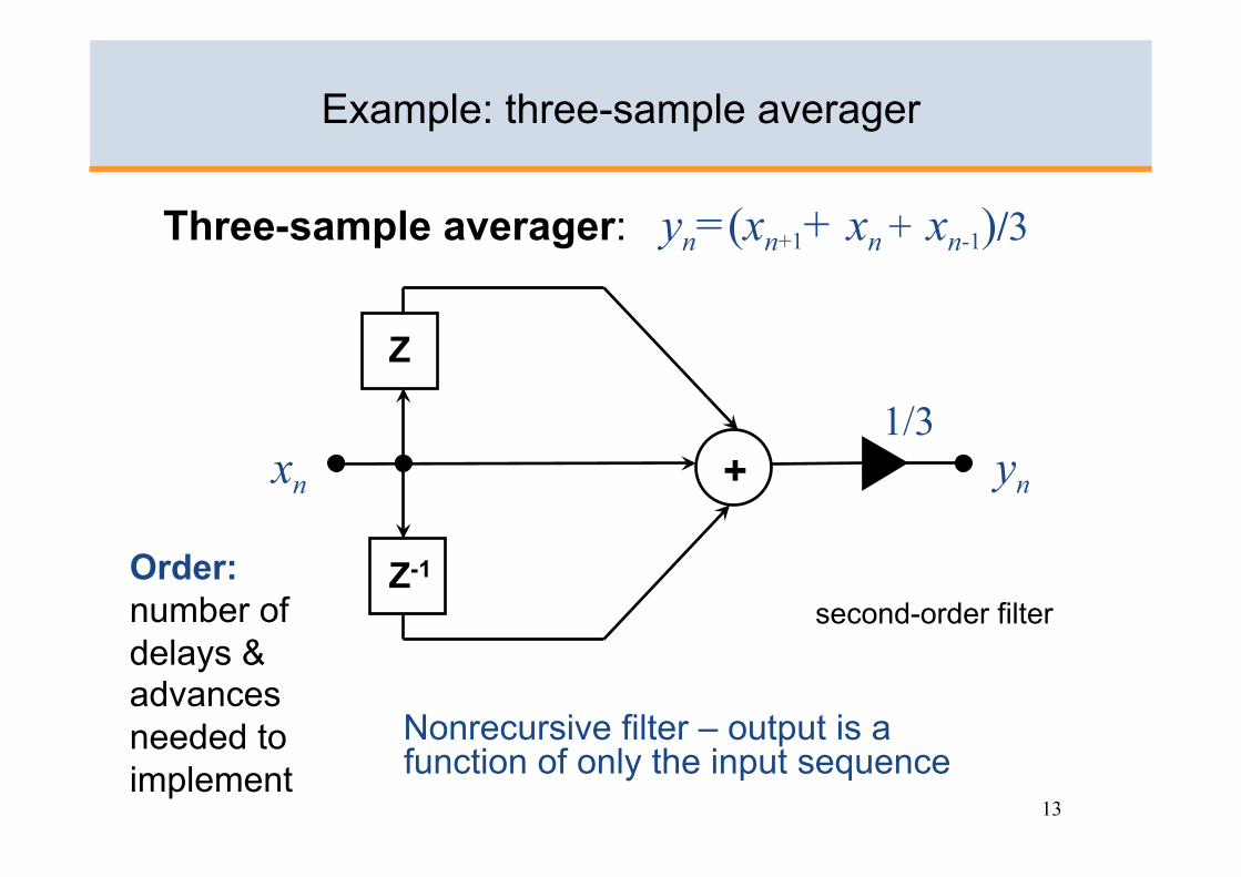
Example: three-sample averager
Nonrecursive filter – output is a function of only the input sequence
Three-sample averager: yn=(xn+1+ xn + xn-1)/3
+ xn
Z-1
Z
yn
1/3
Order: number of delays & advances needed to implement
second-order filter
14
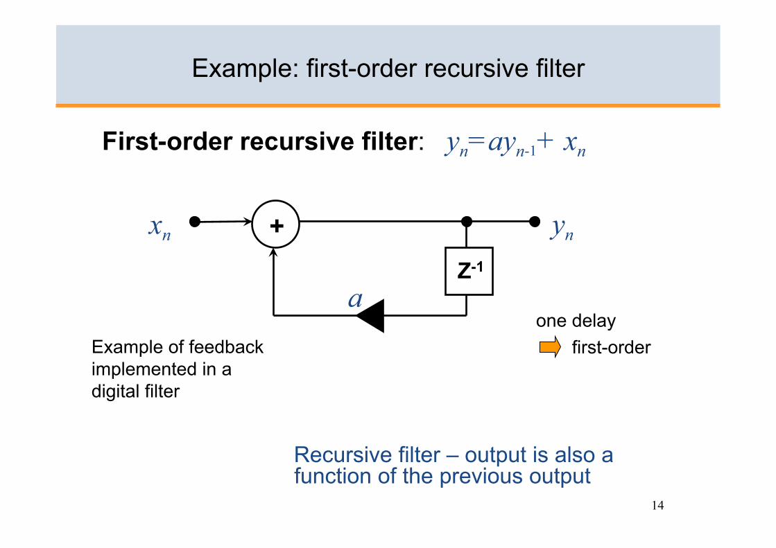
Example: first-order recursive filter
Recursive filter – output is also a function of the previous output
First-order recursive filter: yn=ayn-1+ xn
+ xn yn
Z-1 a
one delay first-order Example of feedback
implemented in a digital filter
15
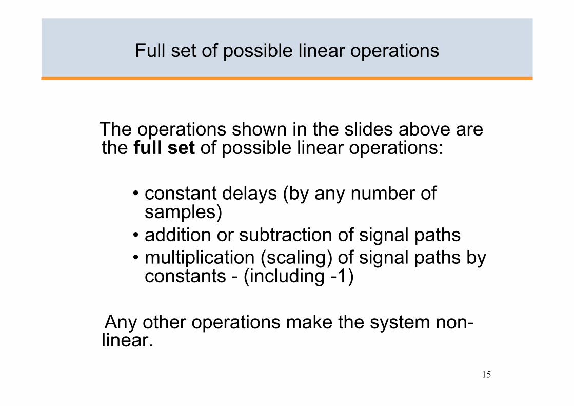
Full set of possible linear operations
The operations shown in the slides above are the full set of possible linear operations:
• constant delays (by any number of samples)
• addition or subtraction of signal paths • multiplication (scaling) of signal paths by
constants - (including -1)
Any other operations make the system non-linear.
16
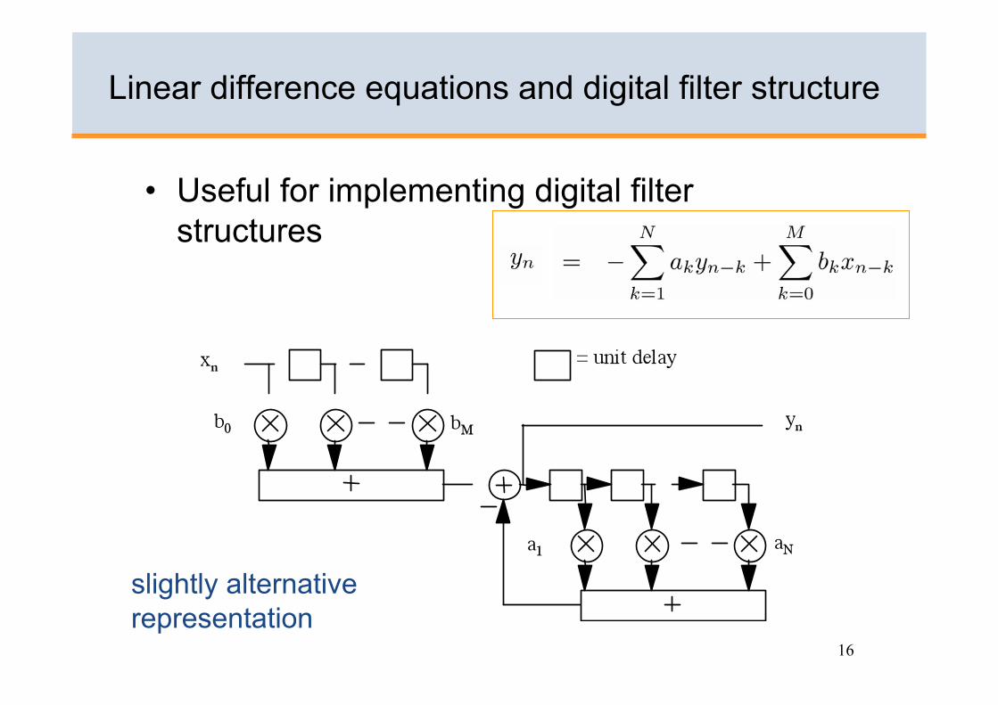
Linear difference equations and digital filter structure
• Useful for implementing digital filter structures
slightly alternative representation

17
Second method in time domain: unit-sample response
• The response of the system to the unit sample sequence is determined
• Taking into account properties of the LTI system, the response of the system to xn is the corresponding sum of weighted outputs
• Input signal is resolved into a weighted sum of elementary signal components, i.e. sum of unit samples or impulses
LTI δn hn
LTI
xn= xk δn-k k = - ∞
∞
xn= xk δn-k k = - ∞
∞ yn= xk hn-k
k = - ∞
∞
18
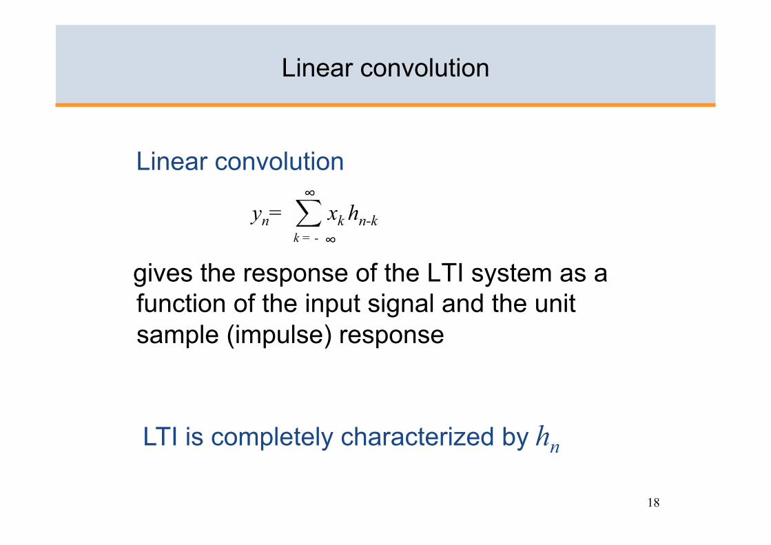
Linear convolution
Linear convolution
gives the response of the LTI system as a function of the input signal and the unit sample (impulse) response
LTI is completely characterized by hn
yn= xk hn-k k = - ∞
∞
19
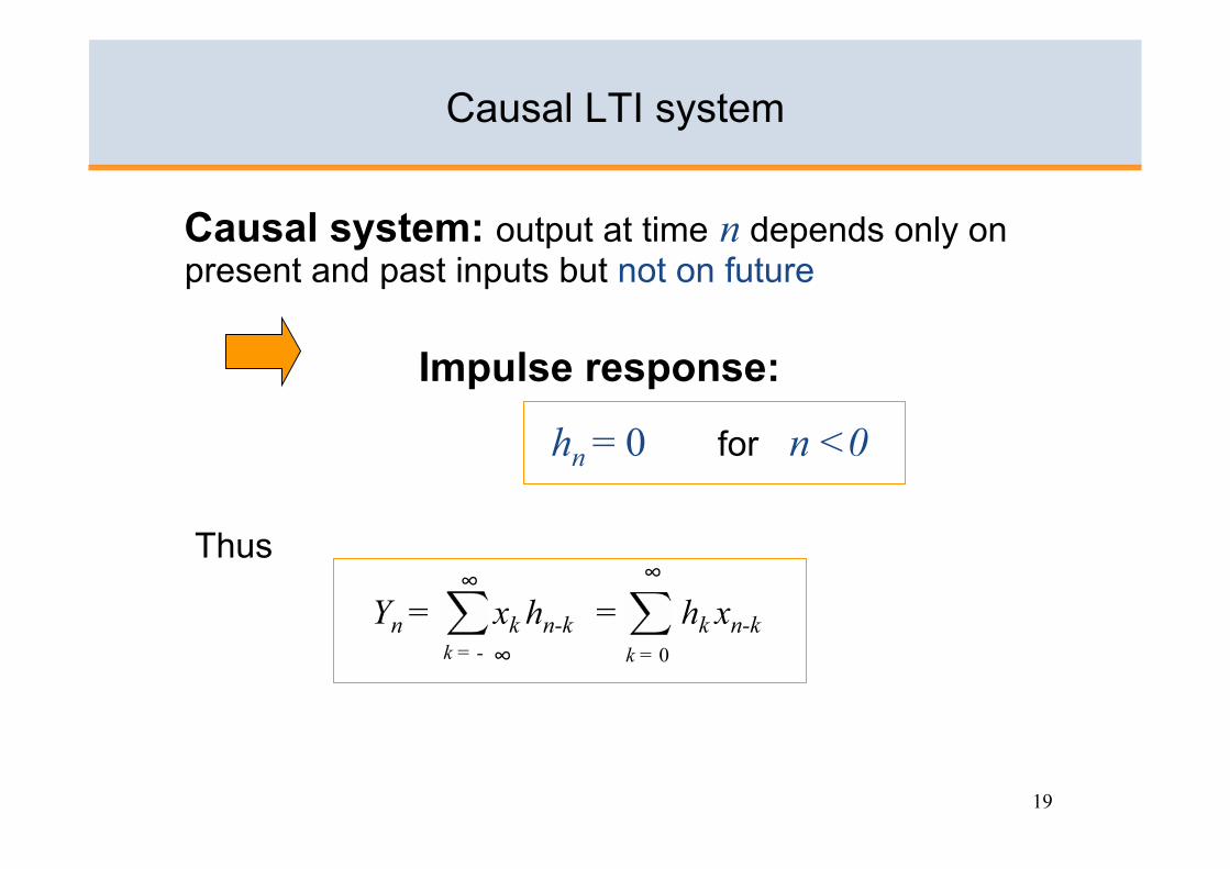
Causal LTI system
Causal system: output at time n depends only on present and past inputs but not on future
Yn = xk hn-k = hk xn-k k = -
hn = 0 for n <0
Impulse response:
Thus
∞
∞
k = 0
∞
20
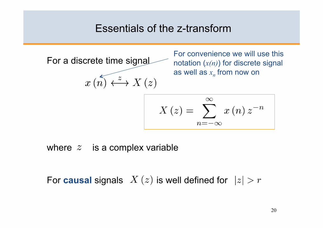
Essentials of the z-transform
For a discrete time signal
where is a complex variable
For causal signals is well defined for
For convenience we will use this notation (x(n)) for discrete signal as well as xn from now on
21
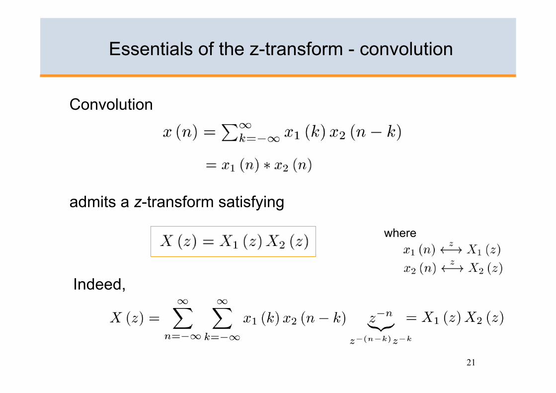
Convolution
Essentials of the z-transform - convolution
admits a z-transform satisfying
Indeed,
where
22
Transfer function of LTI
Linear difference equation
Now, take z-transforms term by term
Rearranging, transfer function of the filter is

23
FIR and IIR filters
Transfer function of the filter is
Finite Impulse Response (FIR) Filters: N = 0, no feedback
Infinite Impulse Response (IIR) Filters
24
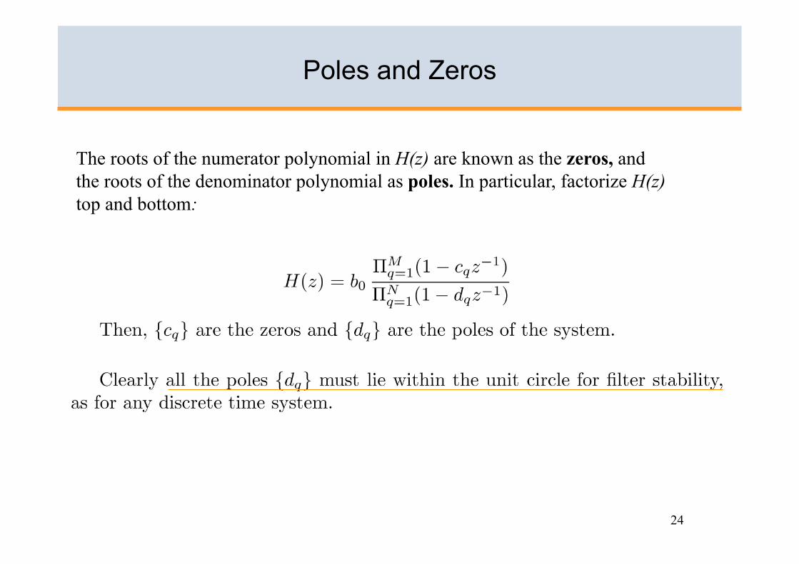
Poles and Zeros
The roots of the numerator polynomial in H(z) are known as the zeros, and the roots of the denominator polynomial as poles. In particular, factorize H(z) top and bottom:

25
Matlab has a filter command for implementation of linear digital filters.
Matlab transfer function:
The format is
y = filter( b, a, x);
where b = [b0 b1 b2 ... bM ]; a = [ 1 a1 a2 a3 ... aN ];
So to compute the first P+1 samples of the filter’s impulse response,
y = filter( b, a, [1 zeros(1,P)]);
Or step response, y = filter( b, a, [ones(1,P)]);
Linear Digital Filter in Matlab
26
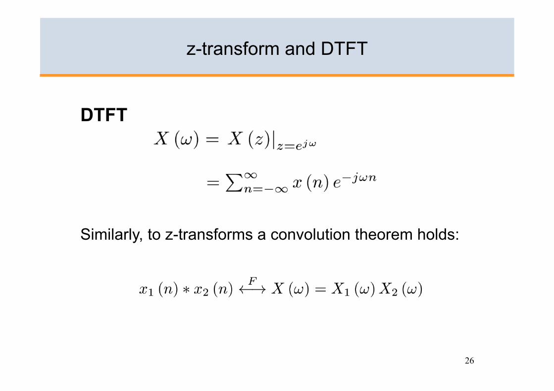
z-transform and DTFT
DTFT
Similarly, to z-transforms a convolution theorem holds:
27
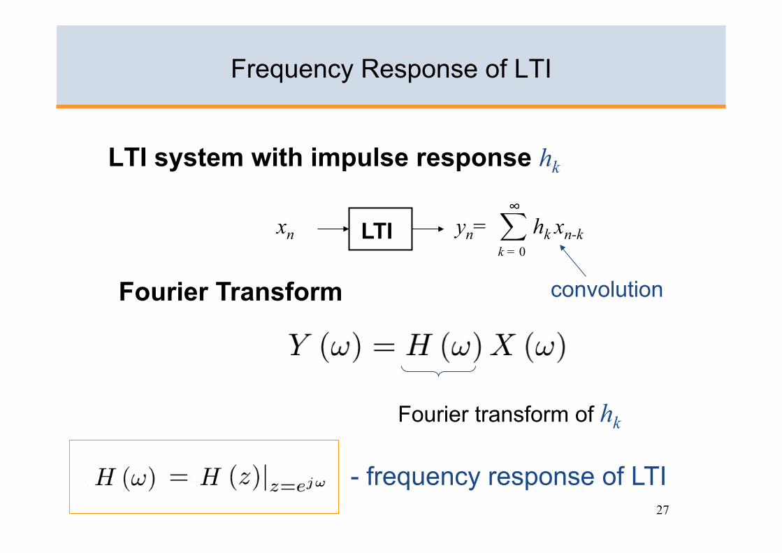
Frequency Response of LTI
LTI system with impulse response hk
LTI xn yn= hk xn-k k = 0
∞
Fourier Transform convolution
Fourier transform of hk
- frequency response of LTI
28
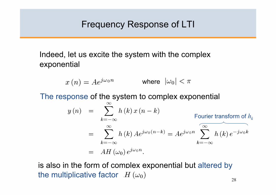
Indeed, let us excite the system with the complex exponential
Frequency Response of LTI
where
The response of the system to complex exponential
Fourier transform of hk
is also in the form of complex exponential but altered by the multiplicative factor
29
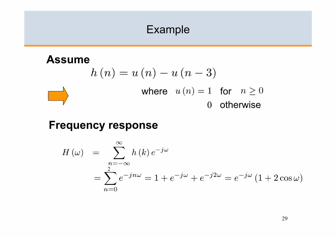
Example
Assume
where for 0 otherwise
2
Frequency response
30
Frequency Response of LTI
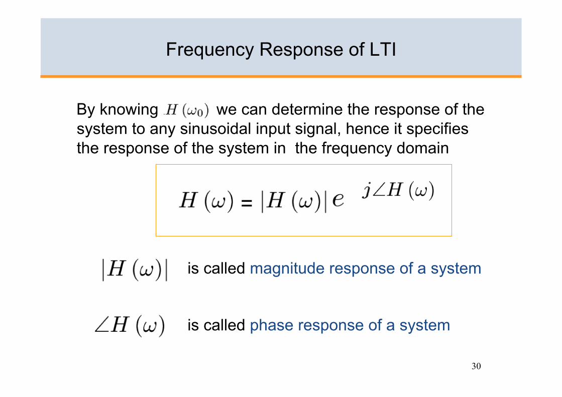
By knowing we can determine the response of the system to any sinusoidal input signal, hence it specifies the response of the system in the frequency domain
is called magnitude response of a system
is called phase response of a system
=
31
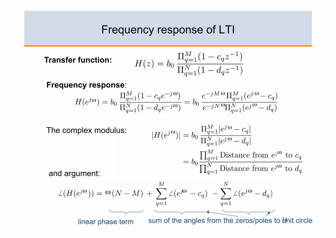
Transfer function:
ωω
ω
ω
ω
ω
ω
Frequency response:
and argument:
ωω
ω
ω
ω
ω ωω ω
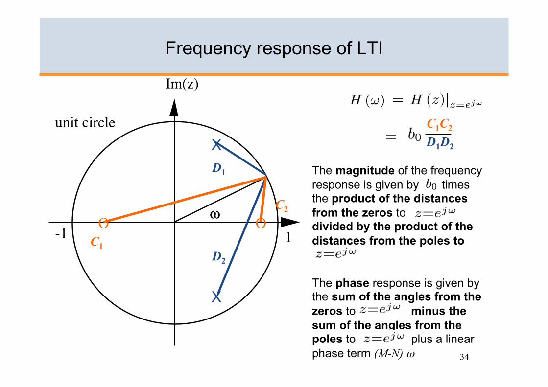
Frequency response of LTI
The complex modulus:
linear phase term sum of the angles from the zeros/poles to unit circle
32
Frequency response of LTI
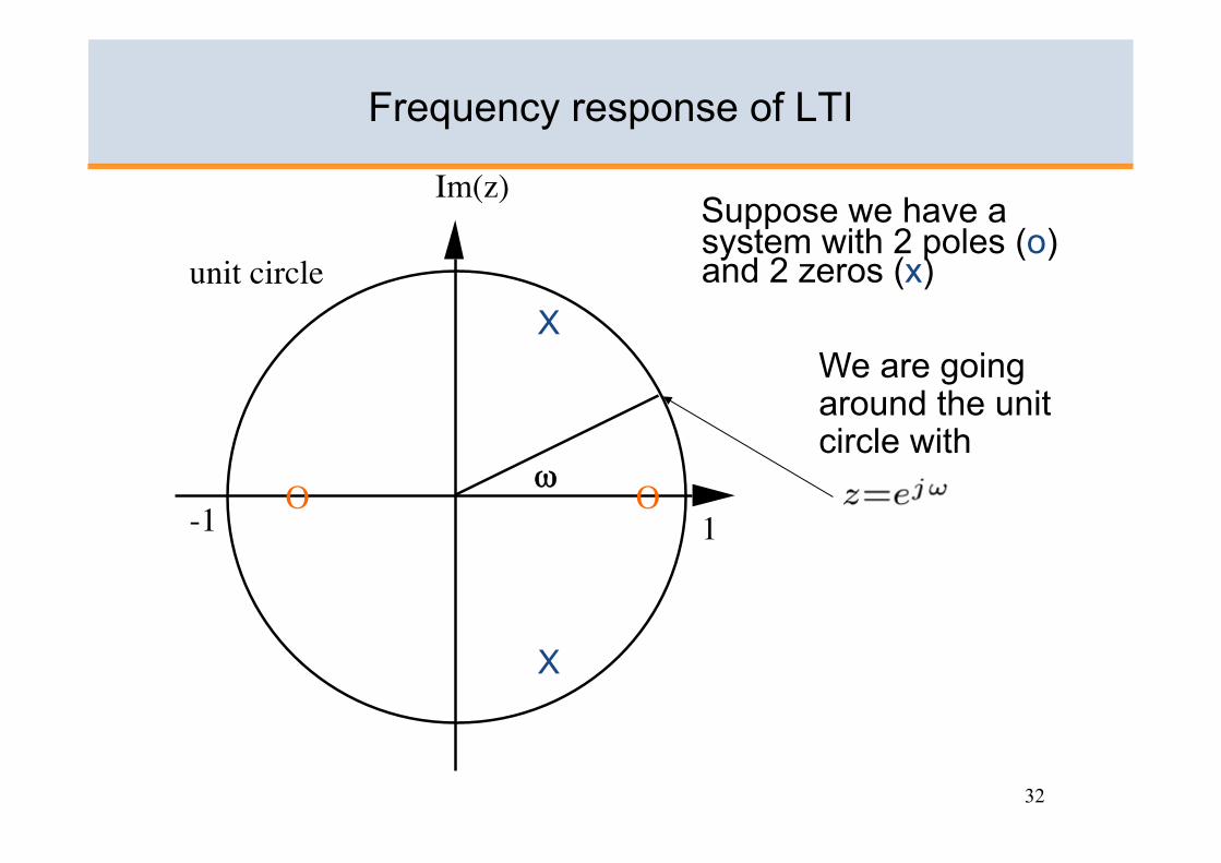
Suppose we have a system with 2 poles (o) and 2 zeros (x)
Im (z)
X
X
O ω
unit circle
O -1 1
We are going around the unit circle with
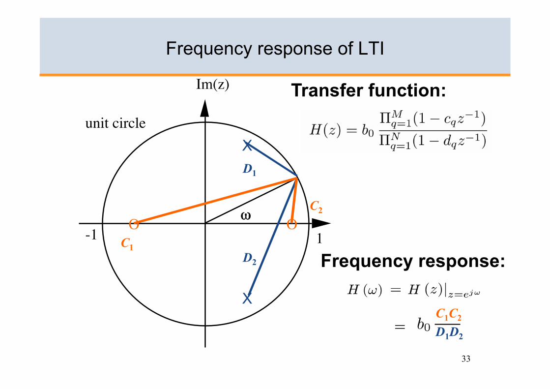
33
Frequency response of LTI
Im (z)
X
X
O ω
unit circle
O -1 1
Transfer function:
Frequency response:
C1C2 D1D2 =
C1
C2
D2
D1
34
Frequency response of LTI
Im (z)
X
X
O ω
unit circle
O -1 1
C1C2 D1D2 =
C1
C2
D2
D1 The magnitude of the frequency response is given by times the product of the distances from the zeros to divided by the product of the distances from the poles to
The phase response is given by the sum of the angles from the zeros to minus the sum of the angles from the poles to plus a linear phase term (M-N) ω
35
Frequency response of LTI
Im (z)
X
X
O ω
unit circle
O -1 1 C1
C2
D2
D1
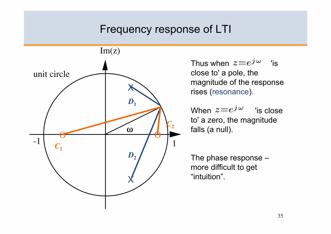
Thus when 'is close to' a pole, the magnitude of the response rises (resonance).
When 'is close to' a zero, the magnitude falls (a null).
The phase response – more difficult to get “intuition”.
36
Frequency response of filter in Matlab
36
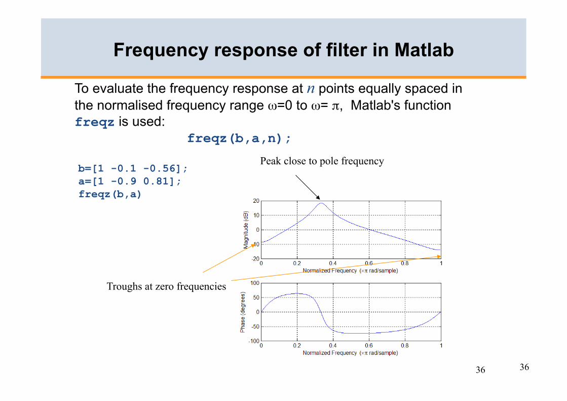
To evaluate the frequency response at n points equally spaced in the normalised frequency range ω=0 to ω= π, Matlab's function freqz is used: freqz(b,a,n);
Peak close to pole frequency
Troughs at zero frequencies
b=[1 -0.1 -0.56]; a=[1 -0.9 0.81]; freqz(b,a)
37 37
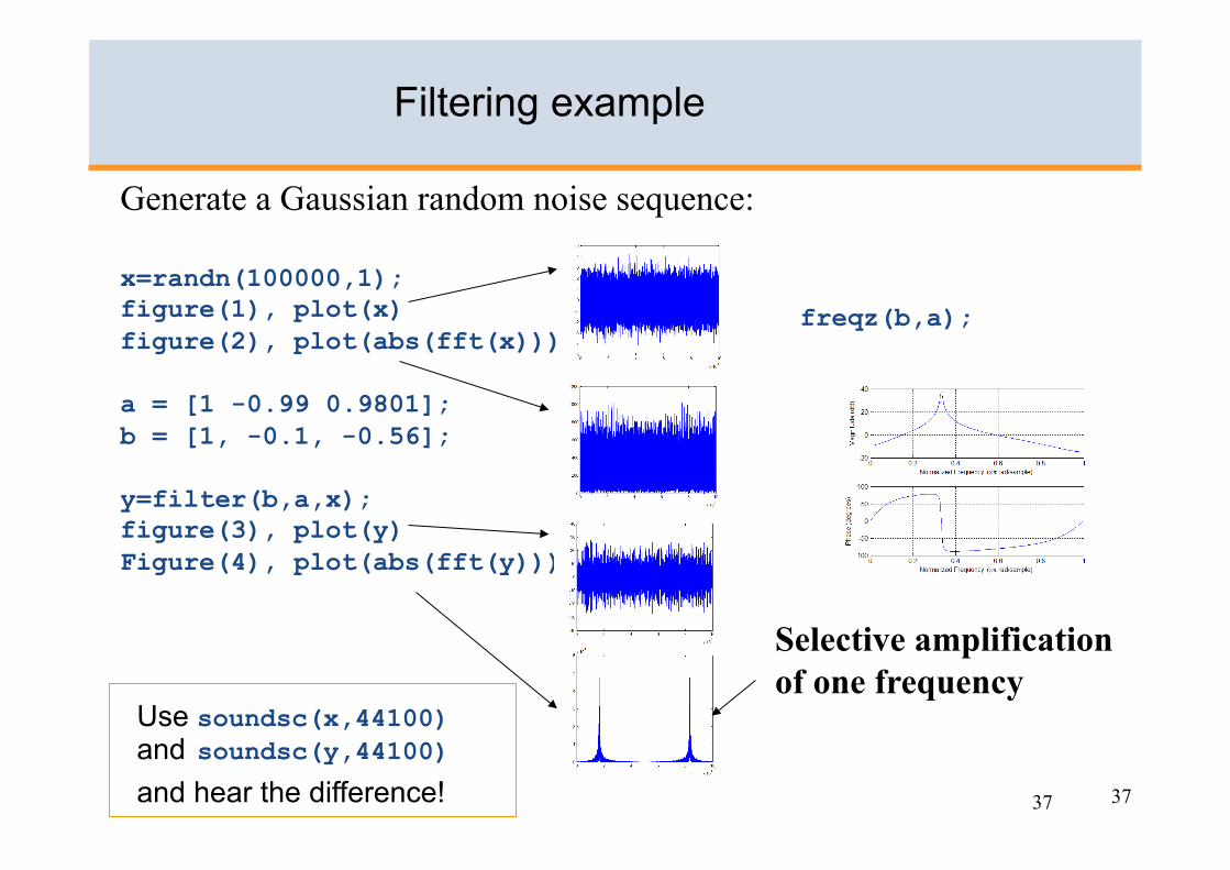
Filtering example
Generate a Gaussian random noise sequence:
x=randn(100000,1); figure(1), plot(x) figure(2), plot(abs(fft(x)))
a = [1 -0.99 0.9801]; b = [1, -0.1, -0.56];
y=filter(b,a,x); figure(3), plot(y) Figure(4), plot(abs(fft(y)))
Selective amplification of one frequency
freqz(b,a);
Use soundsc(x,44100) and soundsc(y,44100) and hear the difference!
38
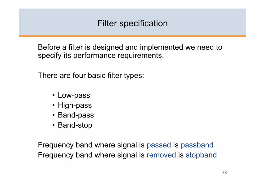
Filter specification
Before a filter is designed and implemented we need to specify its performance requirements.
There are four basic filter types:
• Low-pass • High-pass • Band-pass • Band-stop
Frequency band where signal is passed is passband Frequency band where signal is removed is stopband
39
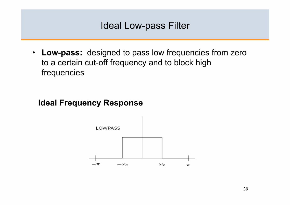
Ideal Low-pass Filter
• Low-pass: designed to pass low frequencies from zero to a certain cut-off frequency and to block high frequencies
Ideal Frequency Response
40
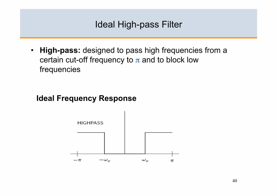
Ideal High-pass Filter
• High-pass: designed to pass high frequencies from a certain cut-off frequency to π and to block low frequencies
Ideal Frequency Response

41
Ideal Band-pass Filter
• Band-pass: designed to pass a certain frequency range which does not include zero and to block other frequencies
Ideal Frequency Response
42
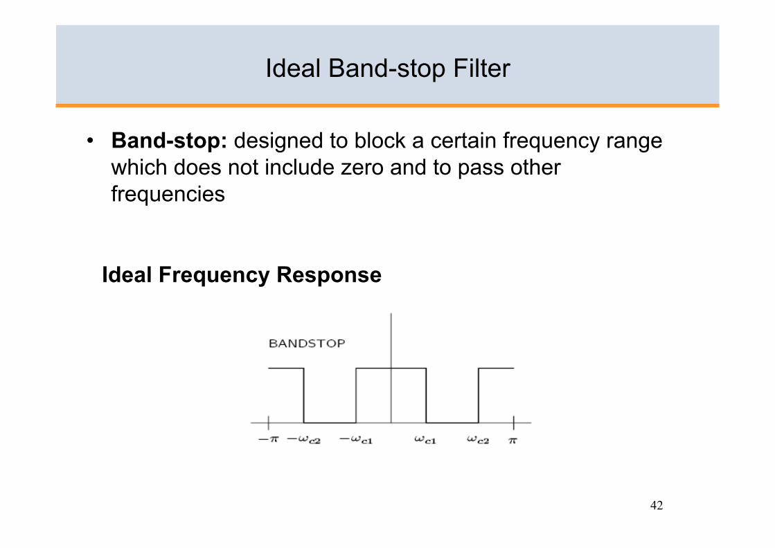
Ideal Band-stop Filter
• Band-stop: designed to block a certain frequency range which does not include zero and to pass other frequencies
Ideal Frequency Response

43
Ideal Filters – Magnitude Response
Ideal Filters are usually such that they admit a gain of 1 in a given passband (where signal is passed) and 0 in their stopband (where signal is removed).
44
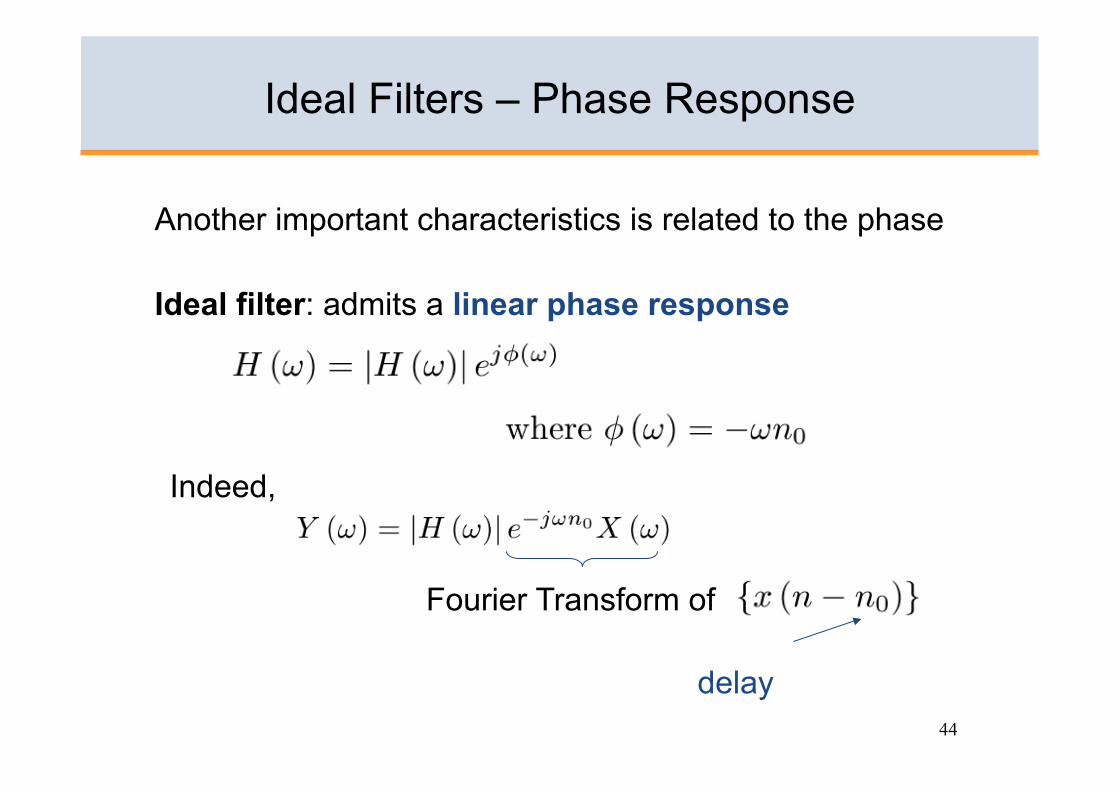
Another important characteristics is related to the phase
Ideal filter: admits a linear phase response
Ideal Filters – Phase Response
Indeed,
Fourier Transform of
delay
45
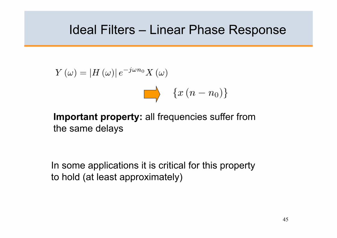
In some applications it is critical for this property to hold (at least approximately)
Ideal Filters – Linear Phase Response
Important property: all frequencies suffer from the same delays
46
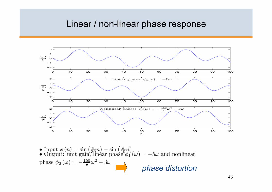
Linear / non-linear phase response
phase distortion
47
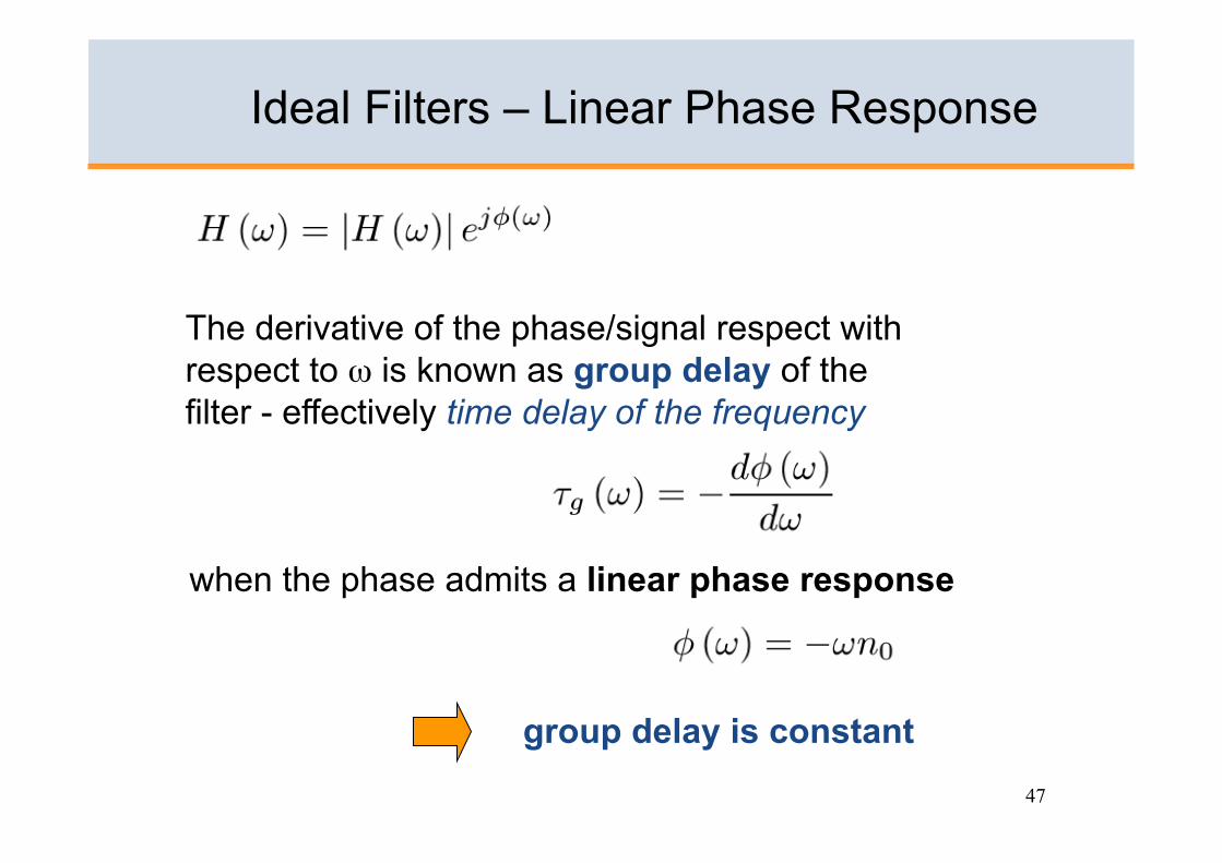
Ideal Filters – Linear Phase Response
The derivative of the phase/signal respect with respect to ω is known as group delay of the filter - effectively time delay of the frequency
when the phase admits a linear phase response
group delay is constant
48
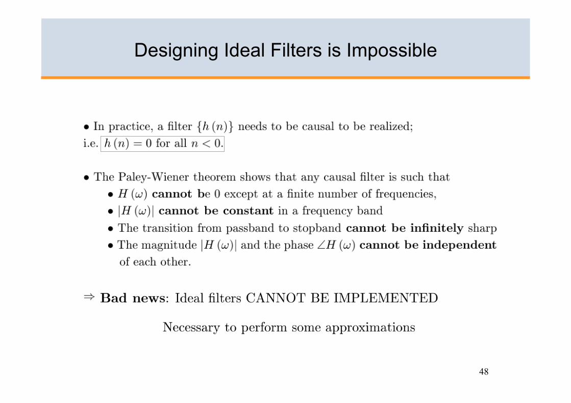
Designing Ideal Filters is Impossible
49
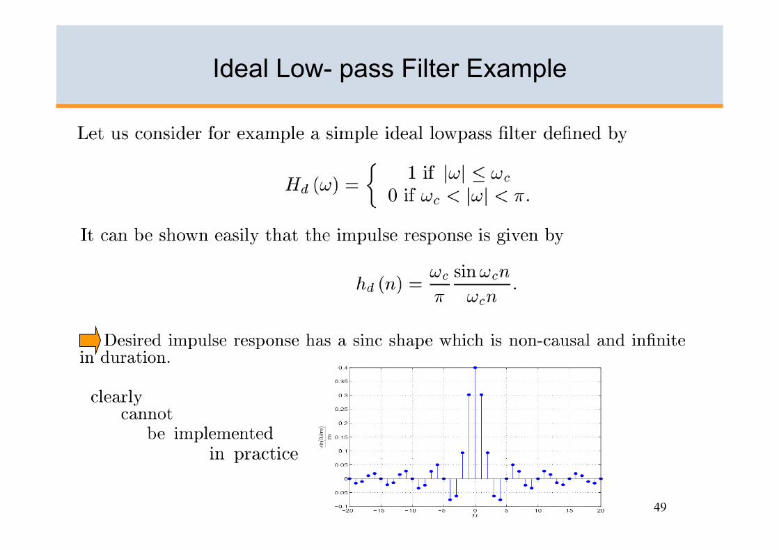
Ideal Low- pass Filter Example
50
Filter Design
Let’s have a go …
51
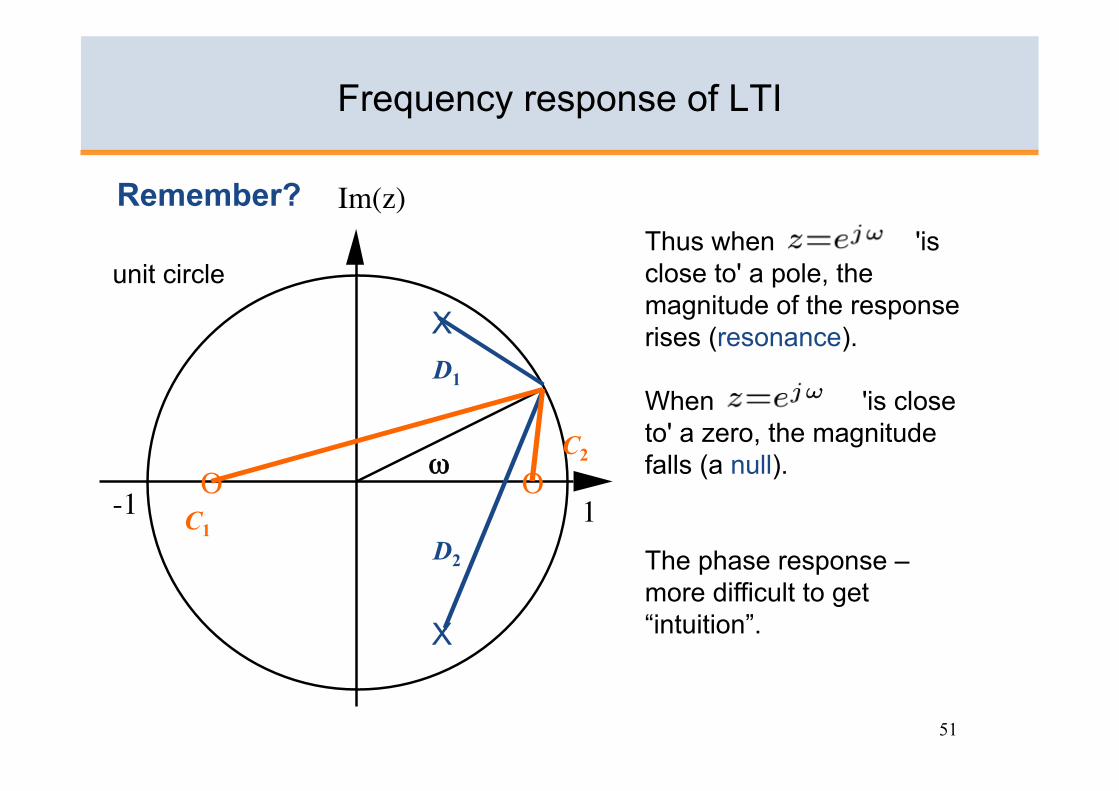
Frequency response of LTI
Im (z)
X
X
O ω
unit circle
O -1 1 C1
C2
D2
D1
Thus when 'is close to' a pole, the magnitude of the response rises (resonance).
When 'is close to' a zero, the magnitude falls (a null).
The phase response – more difficult to get “intuition”.
Remember?
52
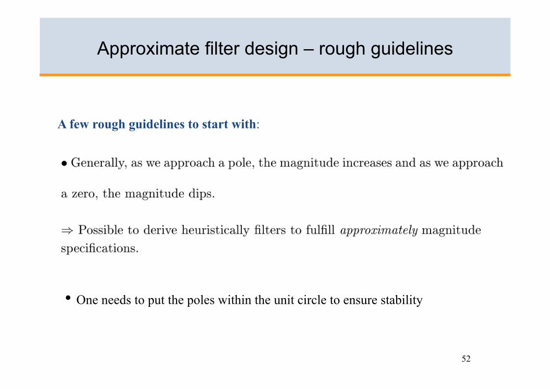
Approximate filter design – rough guidelines
• One needs to put the poles within the unit circle to ensure stability
A few rough guidelines to start with:

53
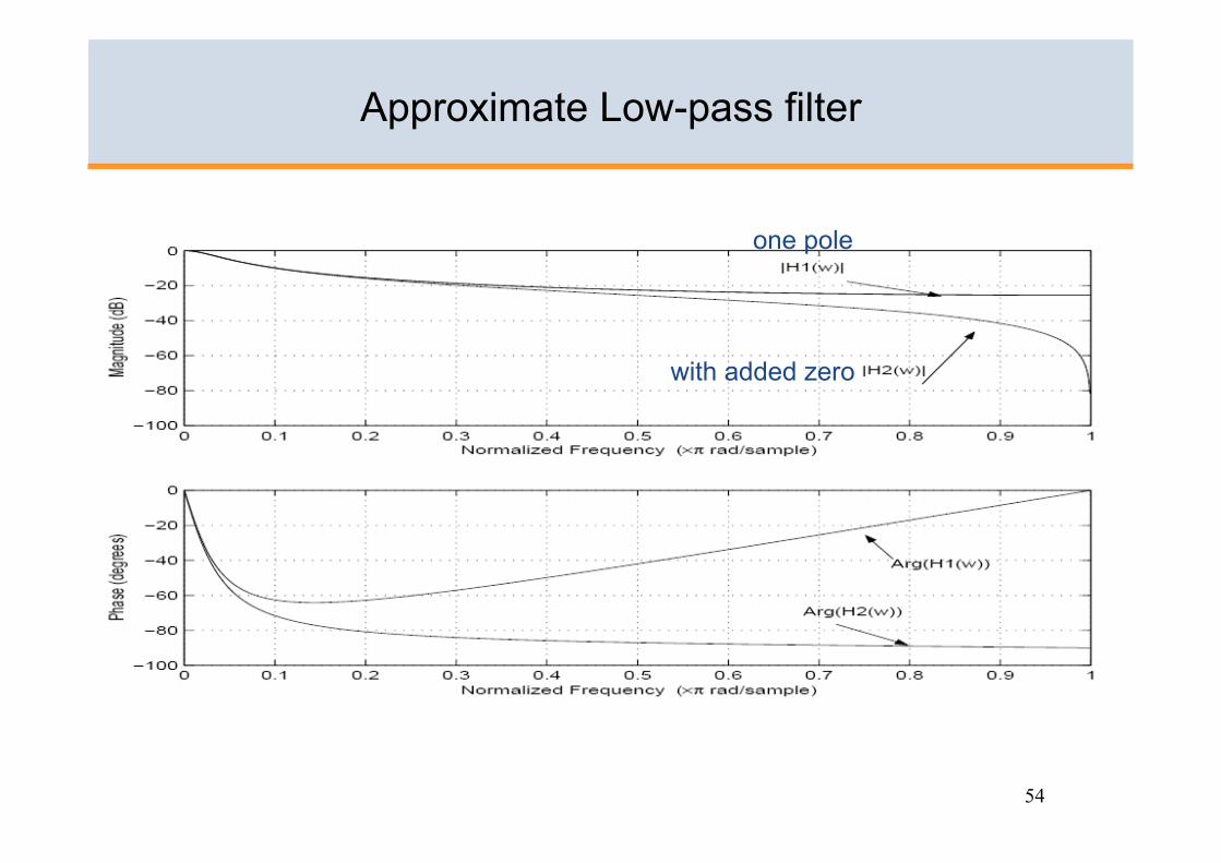
Approximate Low-pass filter
Rule 1: The closer to a pole, the higher the magnitude of the response
Rule 2: The closer to a zero, the lower the magnitude of the response
54
Approximate Low-pass filter
one pole
with added zero
55
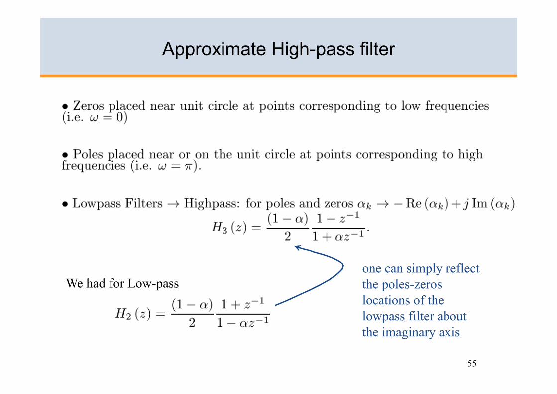
Approximate High-pass filter
one can simply reflect the poles-zeros locations of the lowpass filter about the imaginary axis
We had for Low-pass

56
Approximate High-pass filter
57
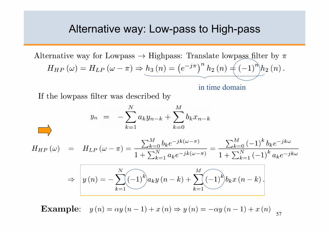
Alternative way: Low-pass to High-pass
in time domain
58
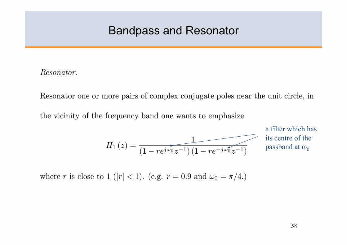
Bandpass and Resonator
a filter which has its centre of the passband at ω0
59
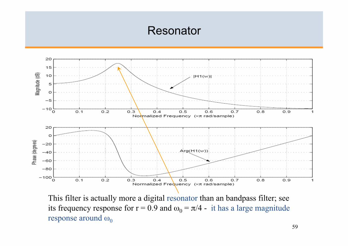
Resonator
This filter is actually more a digital resonator than an bandpass filter; see its frequency response for r = 0.9 and ω0 = π/4 - it has a large magnitude response around ω0

60
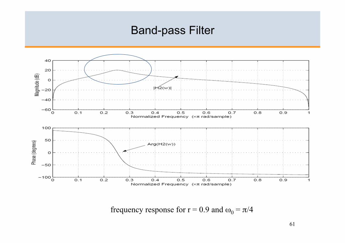
Band-pass Filter
61
Band-pass Filter
frequency response for r = 0.9 and ω0 = π/4
62
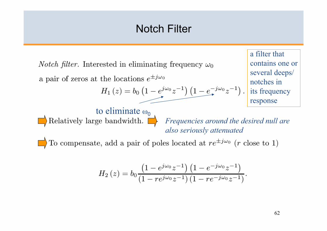
Notch Filter
a filter that contains one or several deeps/ notches in its frequency response
Frequencies around the desired null are also seriously attenuated
to eliminate ω0
63
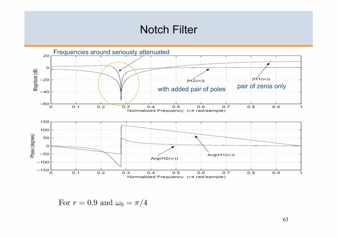
Notch Filter
pair of zeros only with added pair of poles
Frequencies around seriously attenuated
64
All pass Filter
Used as phase equalizer
65
Inverse Filter
The zeros become poles and the poles become zeros
66
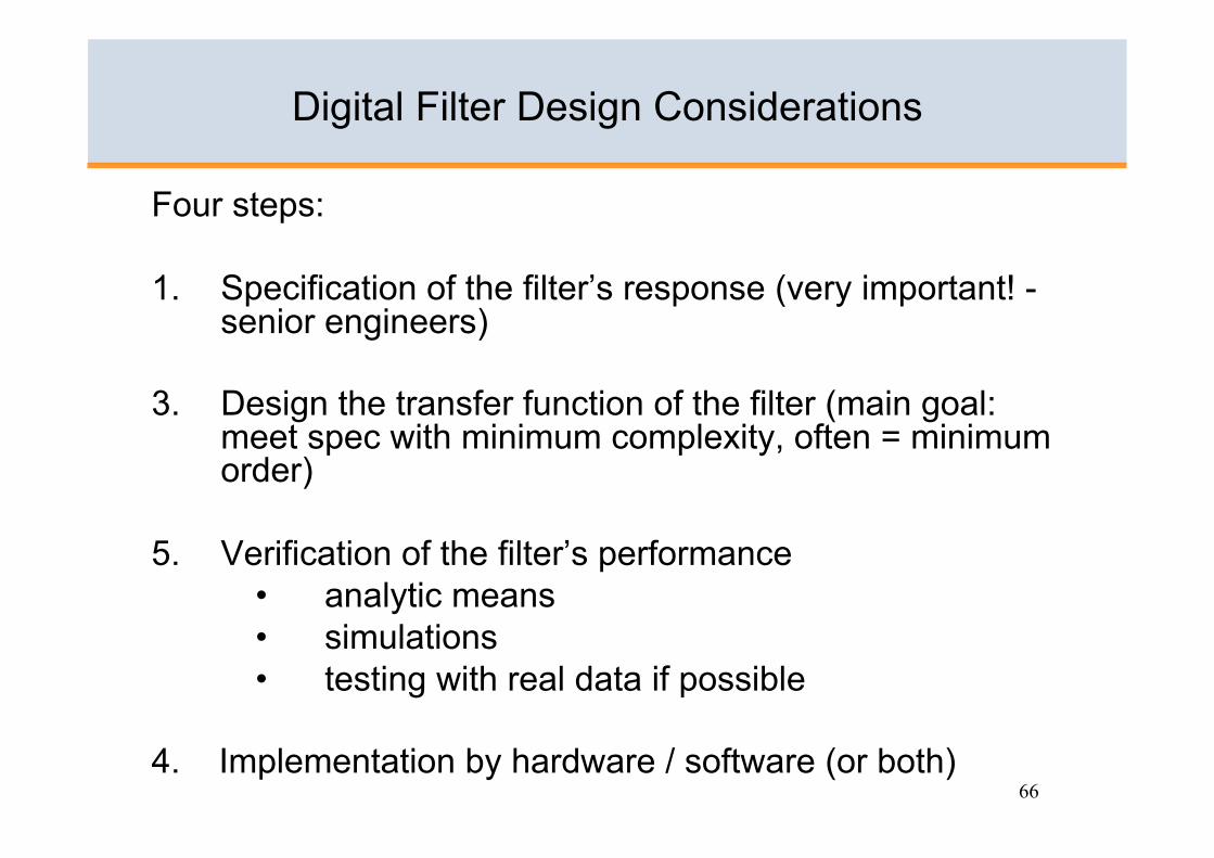
Digital Filter Design Considerations
Four steps:
1. Specification of the filter’s response (very important! - senior engineers)
3. Design the transfer function of the filter (main goal: meet spec with minimum complexity, often = minimum order)
5. Verification of the filter’s performance • analytic means • simulations • testing with real data if possible
4. Implementation by hardware / software (or both)
67
Approximate filter design
Given precise specification what would you do??