4-2 quasi-static fatigue -...

Quasi-Static Fatigue Section 4-2 Step-by-Step Tutorials

1

4-2 Quasi-Static Fatigue Case Description: Composite coupon subject to tensile cyclic loading

Example Location: Tutorials > Fatigue > Quasi Static Fatigue

Model Description:

Nodes: 261; Elements: 224

Length: 1.0” (1.013091”); Width: 0.1964” (0.196248”); and Thickness: 0.10198”

Material Description: Fiber/Matrix (FVR = 55%), with nonlinear matrix stress-strain response

Layup: [0/90/0/90/0/90/0] woven

Objective of Analysis: Predict the fatigue life of the coupon

ASTM Number: -

Control Type: Load Control

Analysis Type: Quasi-Static Fatigue

Solution: *Fatigue 10

(See Section 5 of User Manual)

Input Requirements: GENOA data bank (including experimental stress-strain and S-N curves)

GENOA model files

FEA Solver: MHOST

(Use the keyword *SOLVER as described in Section 5 of User Manual to invoke other FEA solver options such as NASTRAN, ANSYS and ABAQUS)

Output from Analysis: Fatigue life (number of cycles to failure) for three constant load (stress) levels, ply stresses and strains, failure modes at various amounts of cycles

Summary of Results: (a) At the load level of 30% of the ultimate load the fatigue life is 12,500 cycles;

(b) At the load level of 50% of the ultimate load the fatigue life is 3,900 cycles;

(c) At the load level of 70% of the ultimate load the fatigue life is 373.5 cycles


2

Introduction

This tutorial demonstrates how to use GENOA-PFA to estimate the fatigue life of a composite coupon subject to cyclic tension. For details on the technical approach and general features of the code please refer to the GENOA PFA Quick Reference and Theoretical Manuals.

In the example herein, a [0/90/0/90/0/90/0] cross-ply coupon, which is made of the 96-oz 3TEX 3Weave E-glass/Dion 9800TM composite system, is used. The coupon is 1.0 inch long by 0.1964 inch wide by 0.102 inch thick. The analysis is based on the fiber/matrix properties of the composite system. These properties, together with the composite matrix nonlinear stress-strain curve and the S-N degradation curves for the fibers and matrix, were obtained from experiments.

The fatigue life is predicted for the three load (stress) levels with the amplitudes corresponding to approximately 30, 50 and 75 percents of the ultimate static load, which can be determined by running static GENOA-PFA analysis. The simulated results are compared with experimental data.

Launching GENOA

1. Start GENOA by executing it from the desktop or typing genoa in the command prompt.

Importing GENOA Model File

The geometry has already been created in GENOA format as a ‘.dat’ input file.

2. Make sure the Unit System in the upper right corner is set to Inch-Second-Pound.

3. Right click on Quasi Static node under the Fatigue node and select Open Project (see Figure below).

Replace this figure 4. Navigate to the 42ksi directory under Fatigue node under Quasi Static node in the tree.

Note: The FE Model will load in the Mesh view window.


3

Boundary Conditions

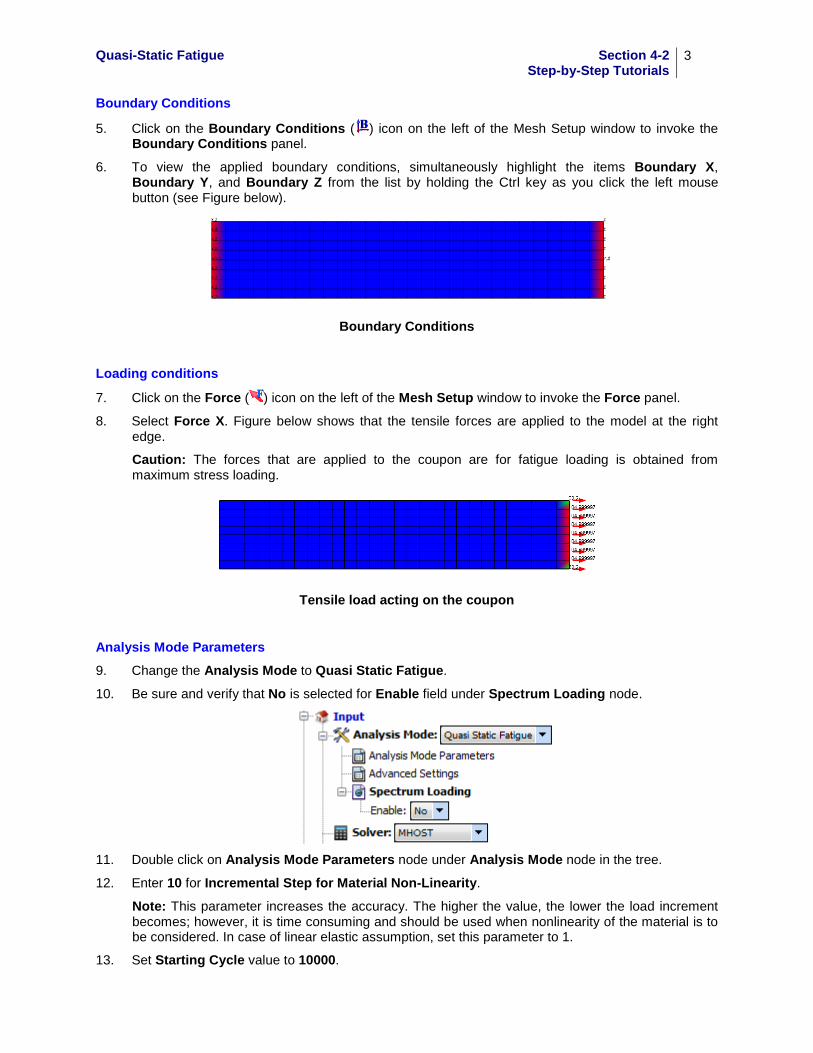
5. Click on the Boundary Conditions ( ) icon on the left of the Mesh Setup window to invoke the Boundary Conditions panel.

6. To view the applied boundary conditions, simultaneously highlight the items Boundary X, Boundary Y, and Boundary Z from the list by holding the Ctrl key as you click the left mouse button (see Figure below).

Boundary Conditions

Loading conditions

7. Click on the Force ( ) icon on the left of the Mesh Setup window to invoke the Force panel.

8. Select Force X. Figure below shows that the tensile forces are applied to the model at the right edge.

Caution: The forces that are applied to the coupon are for fatigue loading is obtained from maximum stress loading.

Tensile load acting on the coupon

Analysis Mode Parameters

9. Change the Analysis Mode to Quasi Static Fatigue.

10. Be sure and verify that No is selected for Enable field under Spectrum Loading node.

11. Double click on Analysis Mode Parameters node under Analysis Mode node in the tree.

12. Enter 10 for Incremental Step for Material Non-Linearity.

Note: This parameter increases the accuracy. The higher the value, the lower the load increment becomes; however, it is time consuming and should be used when nonlinearity of the material is to be considered. In case of linear elastic assumption, set this parameter to 1.

13. Set Starting Cycle value to 10000.


4

Note: If you expect your model to initiate damage at much higher cycles, then you can enter higher starting cycle value. The analysis will attempt to skip the analysis for specified cycles unless there is damage in the FE model. If you are not sure of the starting cycle number, then you are advised to start with Starting Cycle value of 1. The analysis will take longer to run in this condition.

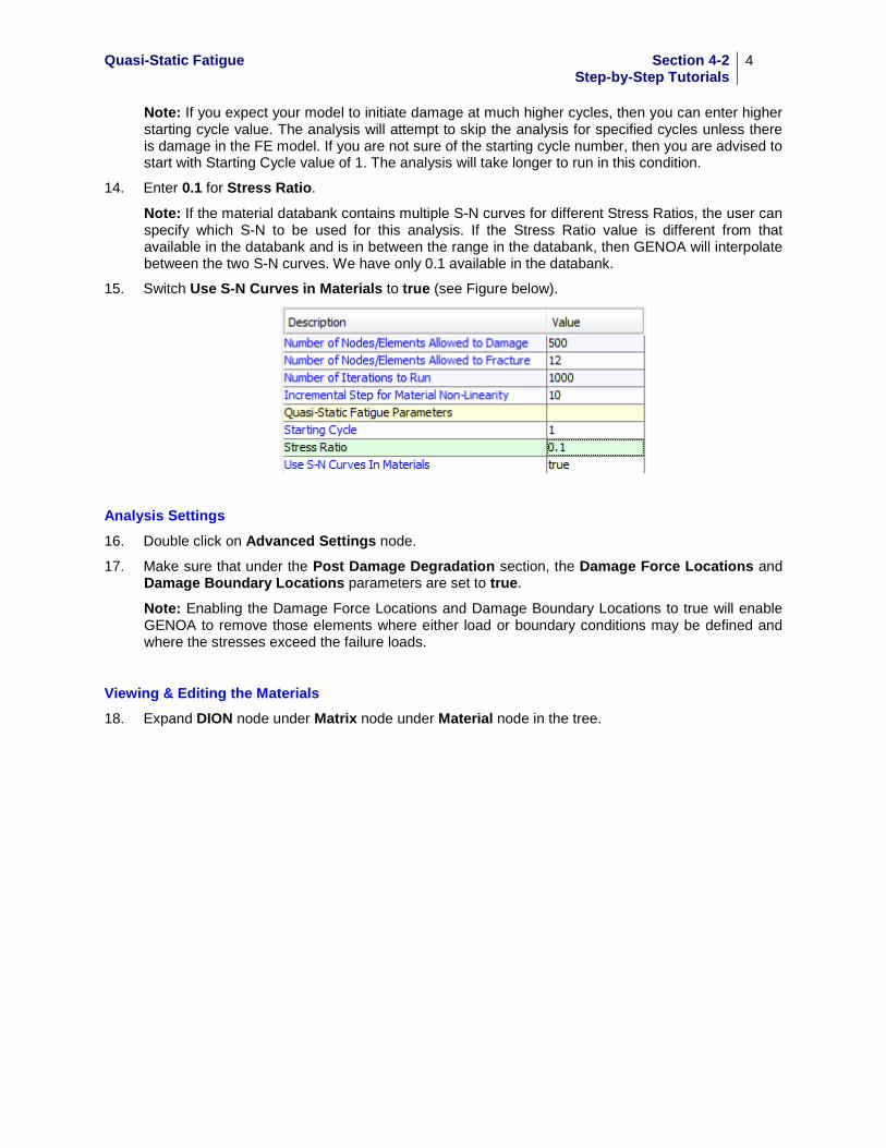
14. Enter 0.1 for Stress Ratio.

Note: If the material databank contains multiple S-N curves for different Stress Ratios, the user can specify which S-N to be used for this analysis. If the Stress Ratio value is different from that available in the databank and is in between the range in the databank, then GENOA will interpolate between the two S-N curves. We have only 0.1 available in the databank.

15. Switch Use S-N Curves in Materials to true (see Figure below).

Analysis Settings

16. Double click on Advanced Settings node.

17. Make sure that under the Post Damage Degradation section, the Damage Force Locations and Damage Boundary Locations parameters are set to true.

Note: Enabling the Damage Force Locations and Damage Boundary Locations to true will enable GENOA to remove those elements where either load or boundary conditions may be defined and where the stresses exceed the failure loads.

Viewing & Editing the Materials

18. Expand DION node under Matrix node under Material node in the tree.


5

19. Double click on Stress Strain Curve node to view the matrix nonlinear stress strain curve.

20. Double click on Stress Cycle Curve node to view matrix degradation curve (SN curve).

Note: Stress ratio value of 0.1 is specified under Stress Cycle Curve node in the tree.


6

Note:

• The S-N data in the databank is entered from lower number of cycles to higher number of cycles.

• In fatigue simulations, materials performance is commonly characterized by a S-N curve (Wöhler curve). The S-N curve is a graph of the magnitude of a cyclical stress (S) against the number of cycles to failure (N). It shows how many cycles are required to cause a fatigue failure for a given nominal stress.

• The S-N relationship is determined for a specified value of stress ratio (R=σmin/σmax).

• The S-N curve is relevant for fatigue failure at high number of cycles (N > 105 cycles).

• If the experimental S-N curve is not available, the bilinear degradation curve can be used instead. In this case, the value of the Use S-N Curves In Databank parameter will be set to false, and the user will be required to input two pairs of coefficients a and b for the expression:

NbaSS log

0

−=

21. Repeat the above steps for EGKG glass fiber material.

Note: usually carbon/graphite/ceramic/aramid fibers show linear behavior; therefore, the SS and S-N curve tabs are left empty. You can create a SN curve if you see degradation in S-N curve for 0 degree ply data subjected to tension-tension axial loading. The S-N curve in this case will represent the reduction in fiber tensile strength due to breakage in the fiber tows.

Laminate Editor

22. Right click on Laminate_1 node under Laminate node in the tree and select Edit in the popup menu.

Note: For this exercise will not modify the laminate.


7

Laminate Editor

Note: The laminate Editor shows that the coupon lay-up consists of 14 composite (EGKGDION) different thickness plies with E-glass fibers arranged in the cross-ply pattern. Also, braid cards are defined which is explained in detail in another tutorial example.

23. Double click on Braid node under Braid (2) node under Materials (4) node in the tree. You will see the vectors defined for up and down going fibers (see Figure below).

Note: the vectors are used to define the out-of-plane orientation of fibers along the x-axis of the ply. Please consult Braid and Woven step-by-step exercise under Static directory for more explanation.

24. Similarly, double click on Braid_1 node under Braid (2) node in the tree.

Note: the vectors are used to define the out-of-plane orientation of fibers along the y-axis of the ply (see Figure below).

25. Click on the Boundary Conditions icon to invoke the Boundary Conditions panel.

Failure Criteria

26. Under the Failure node, double click on FailCrit_1 node to review the damage and failure criteria assigned to the laminates.

27. Click on Composite Default button underneath the Damage Criteria and Critical Failure Criteria tabs.

Note: For this exercise will not modify the Failure Criteria.


8

28. Select Save under Project menu (or press Ctrl and S on the keyboard).

Progressive Failure Analysis

29. Right click on Analysis node and select Progressive Failure Analysis option in the Add popup menu.

30. Right click on Progressive Failure Analysis node and select Run Analysis.

Progressive Failure Analysis Results

Note: After the analysis is completed, the program will automatically switch to the Results Log screen. But if you wish to load the current results during the analysis, then you may choose the


9

Reload Results menu item under the popup menu for the Analysis Results node. You may reload the results at any time if you believe that the results are not current or updated correctly.

When there are results to be loaded, there will be additional nodes under the Analysis Results node as shown below.

Results Log

31. Double click on Results Log node to view the iteration log if not already there after the simulation is complete.

Note: The Results Log table provides information about the amplitude of the applied cyclic load and the number of damaged and fractured nodes corresponding to the number of fatigue cycles. The fatigue cycles corresponding to stable equilibrium are highlighted in green.

32. Click on View All Iterations button. The log will show all the iteration rows (default).

Complete Results Log table

The log indicates that the last equilibrium iteration before fracture corresponds to ~305 cycles, which is the fatigue life of the composite coupon for the stress ratio R = 0.1 and the load amplitude ~838 lbs (nominal stress amplitude ~42 ksi).

Results Mesh

33. Double click on Mesh node in the tree under Analysis Results node.

Note: You will see more nodes under Mesh node in the tree (as shown below).


10

Node Damage

34. Double click on Damage node under Mesh node in the tree.

35. Drag the slider to iteration 5 or enter 5 in the iteration text box.

36. Select Cycles in the drop down list in the player next to iteration text box, as shown in the following Figure.

Note: You will see the following damage modes.

Damage results mesh at Iteration 5 (~78 cycles)

Note: The element switches to red color even if one ply out of 14 plies is damaged.

37. Advance the iterations further until you reach the last iteration.


11

Damage results mesh at Iteration 13 (308 cycles)

Note: The damage panel shows Longitudinal Tension failure that corresponds to fiber failure for 0 degree plies in the coupon. The Longitudinal Compression appears because the fibers in the 90 degree plies are assumed to have buckled during the analysis after matrix failure.

Note: Figures above show that after ~308 cycles of cyclic tensile loading, crack propagation initiation takes place in the composite coupon.

Repeat above steps to predict the fatigue life of the coupon for the load amplitudes ~600 lbs (nominal stress amplitude ~30 ksi) and ~345 lbs (nominal stress amplitude ~17 ksi).

0

10

20

30

40

50

60

1 10 100 1,000 10,000 100,000

Stre

ss [k

si]

Cycles to Failure [Nf]

Test 1

Test 2

GENOA

Fatigue life of the woven composite coupon subject to cyclic tensile loading


12

You have finished the example demonstrating how to use GENOA to predict the fatigue life of a composite structure.

4-2 quasi-static fatigue -...

Documents