4. Capital budgeting and optimal management

(4.1) Capital budgeting as linear programming formulation

(4.2) Cash matching problem

(4.3) Dynamic cash flow processes

(4.4) Harmony theorem – maximum present value criterion and max-

imum return criterion

(4.5) Valuation of a firm

(4.6) Stochastic dominance

1

4.1 Capital budgeting

Allocating a budget among a number of investments or projects.

• Projects or investments that require discrete lumps of cash (un-

like securities where virtually any number of shares can be pur-

chased).

• Assumption: projects are independent where the value of one

project does not depend on another project that is also being

funded.

Suppose there are m potential projects:

bi = total benefit of the ith project (net present value)

ci = initial cost

C = total capital available

2

Define zero-one variable xi =

{

0 if project i is rejected1 if project i is funded

.

Zero-one programming problem

maximizem∑

i=1

bixi

subject tom∑

i=1

cixi ≤ C

xi = 0 or 1 for i = 1,2, · · · , m.

Project can be either selected or not, but for those that are selected,

both the benefits and the costs are directly additive.

3

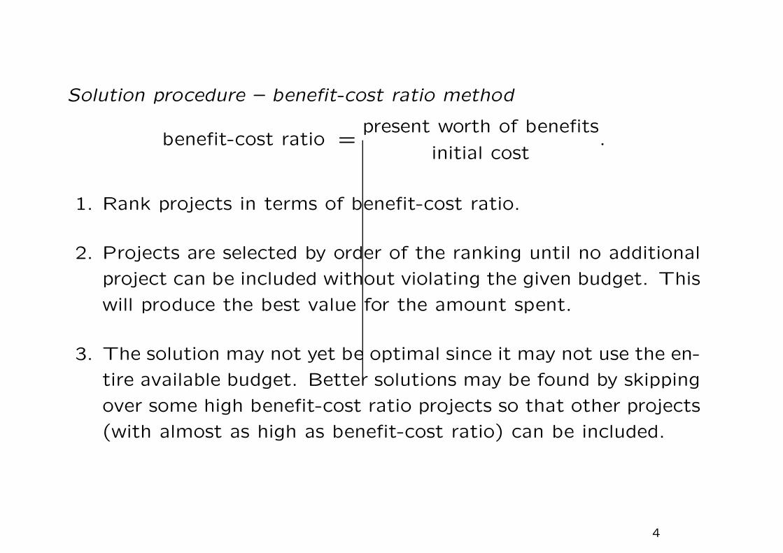
Solution procedure – benefit-cost ratio method

benefit-cost ratio =present worth of benefits

initial cost.

1. Rank projects in terms of benefit-cost ratio.

2. Projects are selected by order of the ranking until no additional

project can be included without violating the given budget. This

will produce the best value for the amount spent.

3. The solution may not yet be optimal since it may not use the en-

tire available budget. Better solutions may be found by skipping

over some high benefit-cost ratio projects so that other projects

(with almost as high as benefit-cost ratio) can be included.

4

Example

$500,000 is made available for the projects listed below:

Project Choices

ProjectOutlay

($1,000)

Present worth

($1,000)

Benefit-cost ratio

1 100 300 3.002 20 50 2.503 150 350 2.334 50 110 2.205 50 100 2.006 150 250 1.677 150 200 1.33

Using the simple benefit-cost ratio ranking method, Projects 1, 2,

3, 4 and 5 are selected for a total expenditure of $370,000, and a

present value of

$910,000 − $370,000 = $540,000.

5

Formulation

maximize 200x1 + 30x2 + 200x3 + 60x4 + 50x5 + 100x6 + 50x7

subject to 100x1 + 20x2 + 150x3 + 50x4 + 50x5 + 150x6 + 150x7 ≤ 500

xi = 0 or 1 for each i.

Note that the terms of the objective for maximization are present

worth minus outlay — present value.

The solution is to select Projects 1,3,4,5 and 6 for a total expen-

diture of $500,000 and a total net present value $610,000.

6

Project Outlay

Present

worth Net PV

Optimal

x -value Cost Optimal PV

1 100 300 200 1 100 200

2 20 50 30 0 0 0

3 150 350 200 1 150 200

4 50 110 60 1 50 60

5 50 100 50 1 50 50

6 150 250 100 1 150 100

7 150 200 50 0 0 0

Totals 500 610

7

Interdependent projects

• Sometimes various projects are interdependent, the feasibility of

one being dependent on whether others are undertaken.

• Suppose a transportation authority wishes to construct a road

between two cities. Corresponding projects might detail whether

the road were concrete or asphalt, two lanes or four, and so

forth. Another, independent goal might be the improvement of

a bridge.

• In general, assume that there are m goals and that associated

with the ith goal there are ni possible projects. Only one project

can be selected for any goal. As before, there is a fixed available

budget.

8

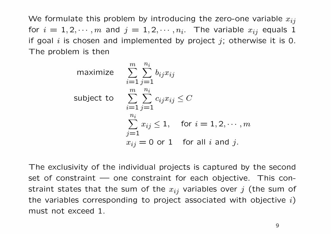
We formulate this problem by introducing the zero-one variable xij

for i = 1,2, · · · , m and j = 1,2, · · · , ni. The variable xij equals 1

if goal i is chosen and implemented by project j; otherwise it is 0.

The problem is then

maximizem∑

i=1

ni∑

j=1

bijxij

subject tom∑

i=1

ni∑

j=1

cijxij ≤ C

ni∑

j=1

xij ≤ 1, for i = 1,2, · · · , m

xij = 0 or 1 for all i and j.

The exclusivity of the individual projects is captured by the second

set of constraint — one constraint for each objective. This con-

straint states that the sum of the xij variables over j (the sum of

the variables corresponding to project associated with objective i)

must not exceed 1.

9

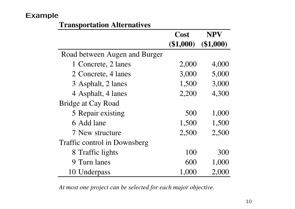
Example

Transportation Alternatives

Cost

($1,000)

NPV

($1,000)

1 Concrete, 2 lanes 2,000 4,000

2 Concrete, 4 lanes 3,000 5,000

3 Asphalt, 2 lanes 1,500 3,000

4 Asphalt, 4 lanes 2,200 4,300

Bridge at Cay Road

5 Repair existing 500 1,000

6 Add lane 1,500 1,500

7 New structure 2,500 2,500

Traffic control in Downsberg

8 Traffic lights 100 300

9 Turn lanes 600 1,000

10 Underpass 1,000 2,000

At most one project can be selected for each major objective.

Road between Augen and Burger

10

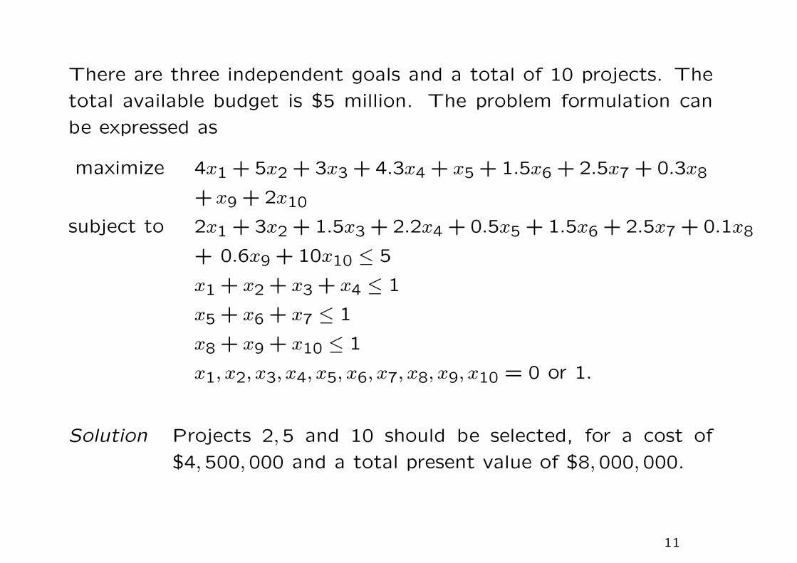
There are three independent goals and a total of 10 projects. The

total available budget is $5 million. The problem formulation can

be expressed as

maximize 4x1 + 5x2 + 3x3 + 4.3x4 + x5 + 1.5x6 + 2.5x7 + 0.3x8

+x9 + 2x10

subject to 2x1 + 3x2 + 1.5x3 + 2.2x4 + 0.5x5 + 1.5x6 + 2.5x7 + 0.1x8

+ 0.6x9 + 10x10 ≤ 5

x1 + x2 + x3 + x4 ≤ 1

x5 + x6 + x7 ≤ 1

x8 + x9 + x10 ≤ 1

x1, x2, x3, x4, x5, x6, x7, x8, x9, x10 = 0 or 1.

Solution Projects 2,5 and 10 should be selected, for a cost of

$4,500,000 and a total present value of $8,000,000.

11

Project

Cost

($1,000)

NPV

($1,000)

Optimal

x-values Cost NPV Goals

1 Concrete, 2 lanes 2,000 4,000 0 0 0

2 Concrete, 4 lanes 3,000 5,000 1 3,000 5,000

3 Asphalt, 2 lanes 1,500 3,000 0 0 0

4 Asphalt, 4 lanes 2,200 4,300 0 0 0 1

5 Repair existing 500 1,000 1 500 1,000

6 Add lane 1,500 1,500 0 0 0

7 New structure 2,500 2,000 0 0 0 1

8 Traffic lights 100 300 0 0 0

9 Turn lanes 600 1,000 0 0 0

10 Underpass 1,000 2,000 1 1,000 2,000 1

Totals 4,500 8,000

12

Remarks

• This method for treating dependencies among projects can be

extended to situations where precedence relations apply (that is,

where one project cannot be chosen unless another is also cho-

sen) and to capital budgeting problems with additional financial

constraints.

• The hard budget constraint is inconsistent with the underlying

assumption that it is possible for the investor (or organization)

to borrow unlimited funds at a given interest rate. In theory

one should carry out all projects that have positive net present

value.

• The assumption that an unlimited supply of capital is available

at a fixed interest rate does not hold. It is usually worth solving

the problem for various values of the budget to measure the

sensitivity of the benefit to the budget level.

13

4.2 Cash matching problems

• We face a known sequence of future monetary obligations. If

we manage a pension fund, these obligations might represent

required annuity payments.

• We wish to invest now so that these obligations can be met

as they occur; and accordingly, we plan to purchase bonds of

various maturities and use the coupon payments and redemption

values to meet the obligations.

• The simplest approach is to design a portfolio that will, without

future alteration, provide the necessary cash as required.

• Only portfolios of fixed-income instruments are considered. A

fixed-income instrument that returns cash at known points in

time can be described by listing the stream of promised cash

payments (and future cash outflows, if any).

14

• We establish a basic time period length, with cash flows occur-

ring at the end of these periods. Our obligation is then a stream

y = (y1, y2, · · · , yn), starting one period from now.

• Each bond has an associated cash flow stream of receipts,

starting one period from now. If there are m bonds, we de-

note the stream associated with one unit of bond j by cj =

(c1j, c2j, · · · cnj).

• The price of bond j is denoted by pj. We denote by xj the

amount of bond j to be held in the portfolio.

15

The cash matching problem is to find the xj’s of minimum total

cost that guarantee that the obligations can be met. Specifically,

minimizem∑

j=1

pjxj

subject tom∑

j=1

cijxj ≥ yi for i = 1,2, · · · , n

xj ≥ 0 for j = 1,2, · · · , m.

The main set of constraints are the cash matching constraints. The

final constraint rules out the possibility of selling bonds short.

16

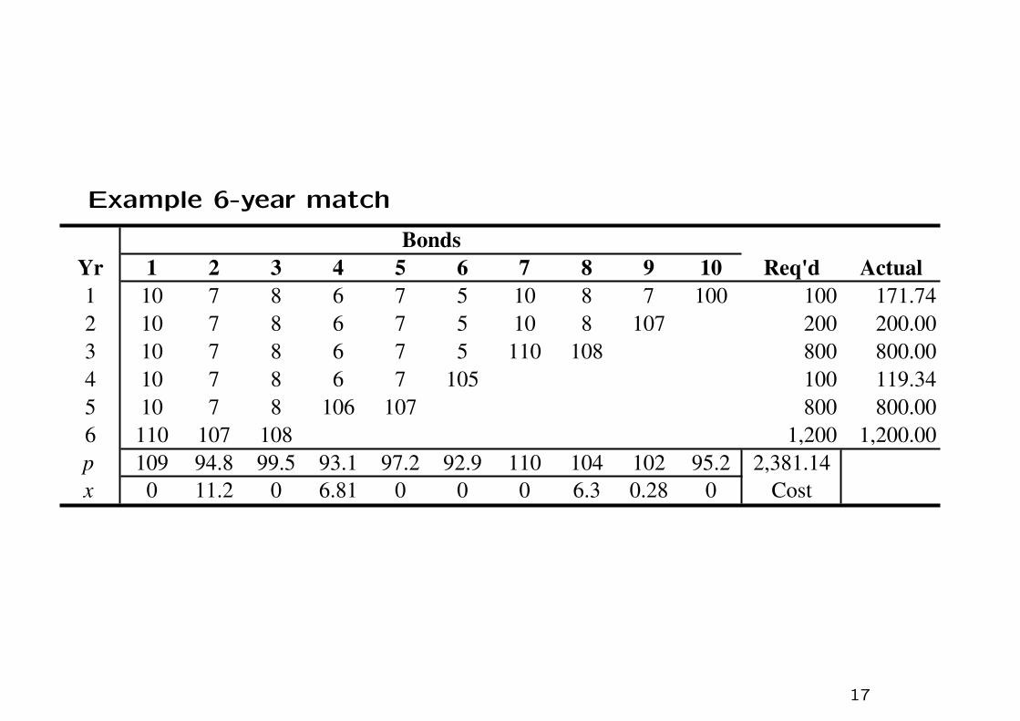
Example 6-year match

Yr 1 2 3 4 5 6 7 8 9 10 Req'd Actual

1 10 7 8 6 7 5 10 8 7 100 100 171.74

2 10 7 8 6 7 5 10 8 107 200 200.00

3 10 7 8 6 7 5 110 108 800 800.00

4 10 7 8 6 7 105 100 119.34

5 10 7 8 106 107 800 800.00

6 110 107 108 1,200 1,200.00

p 109 94.8 99.5 93.1 97.2 92.9 110 104 102 95.2 2,381.14

x 0 11.2 0 6.81 0 0 0 6.3 0.28 0 Cost

Bonds

17

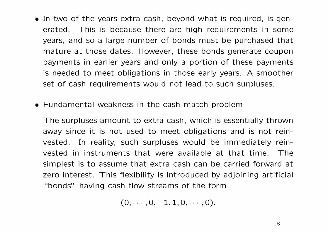
• In two of the years extra cash, beyond what is required, is gen-

erated. This is because there are high requirements in some

years, and so a large number of bonds must be purchased that

mature at those dates. However, these bonds generate coupon

payments in earlier years and only a portion of these payments

is needed to meet obligations in those early years. A smoother

set of cash requirements would not lead to such surpluses.

• Fundamental weakness in the cash match problem

The surpluses amount to extra cash, which is essentially thrown

away since it is not used to meet obligations and is not rein-

vested. In reality, such surpluses would be immediately rein-

vested in instruments that were available at that time. The

simplest is to assume that extra cash can be carried forward at

zero interest. This flexibility is introduced by adjoining artificial

“bonds” having cash flow streams of the form

(0, · · · ,0,−1,1,0, · · · ,0).

18

4.3 Dynamic cash flow processes

Many investments require deliberate ongoing management.

Example

You have purchased an oil well, you must decide, each month,

whether to pump oil from your well or not.

• If you do pump oil, you will incur operational costs and receive

revenue from the sale of oil, leading to a profit; but you will also

reduce the oil reserves.

• If you believe that current oil prices are low, you may wisely

choose not to pump now, but rather to save the oil for a time

for higher prices.

19

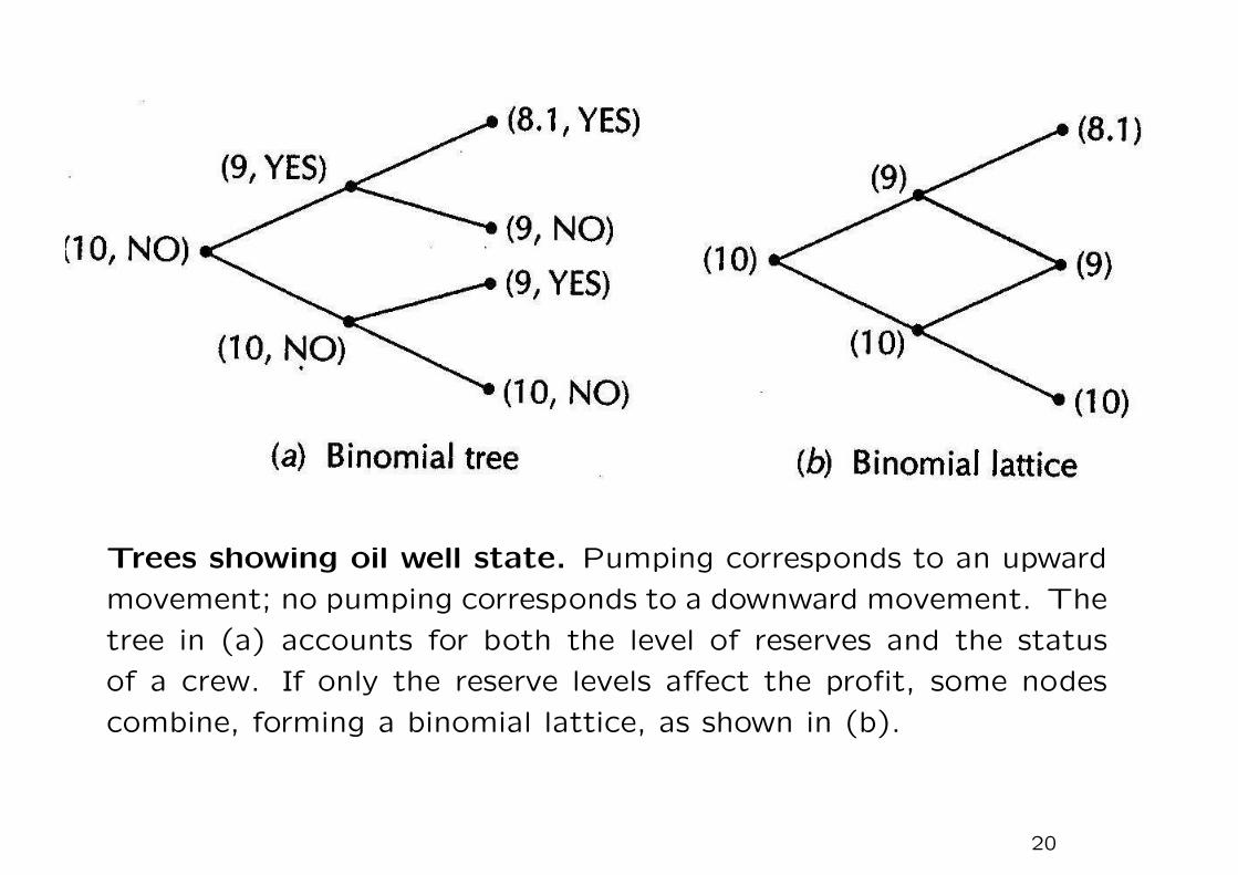
Trees showing oil well state. Pumping corresponds to an upward

movement; no pumping corresponds to a downward movement. The

tree in (a) accounts for both the level of reserves and the status

of a crew. If only the reserve levels affect the profit, some nodes

combine, forming a binomial lattice, as shown in (b).

20

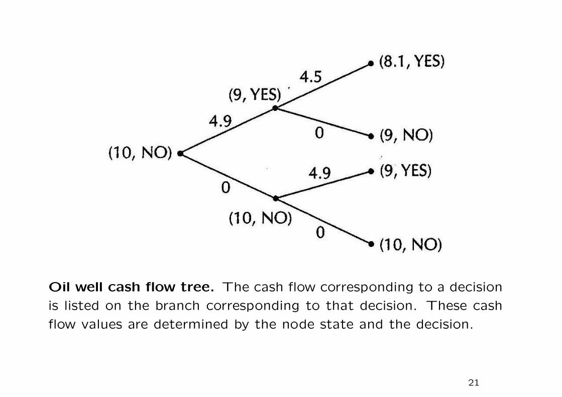
Oil well cash flow tree. The cash flow corresponding to a decision

is listed on the branch corresponding to that decision. These cash

flow values are determined by the node state and the decision.

21

Example – Fishing problem

1. If you do not fish, the fish population will double by the start

of the next season. If you do fish, you will extract 70% of the

fish that were in the lake at the beginning of the season. The

fish that were not caught (and some before they are caught)

will reproduce, the fish population at the beginning of the next

season will be same as at the beginning of the current season.

2. The initial fish population is 10 tons. Your profit is $1 per ton.

The interest rate is constant at 25%, so that the discount factor

is 0.8 each year.

3. You have only three seasons to fish. The management problem

is that of determining in which of those seasons you should fish.

22

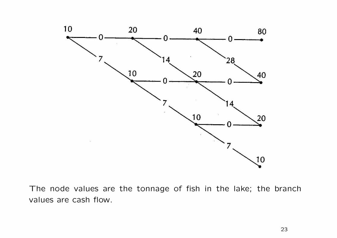
The node values are the tonnage of fish in the lake; the branch

values are cash flow.

23

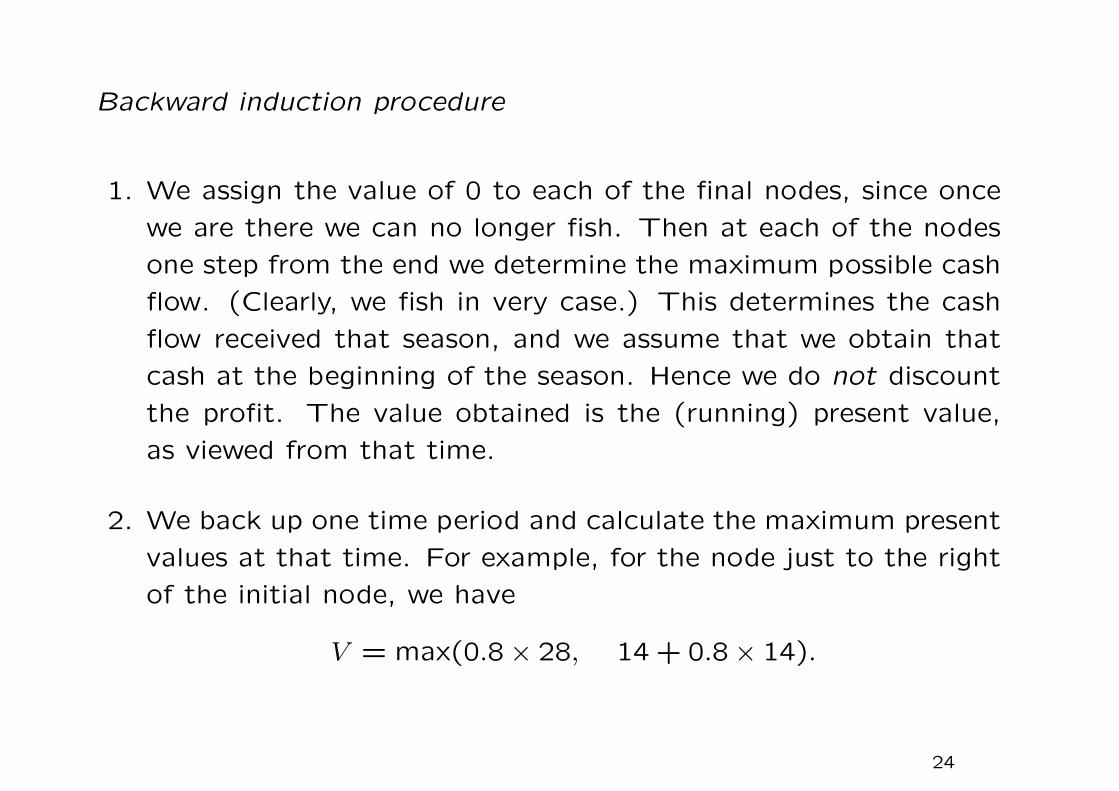
Backward induction procedure

1. We assign the value of 0 to each of the final nodes, since once

we are there we can no longer fish. Then at each of the nodes

one step from the end we determine the maximum possible cash

flow. (Clearly, we fish in very case.) This determines the cash

flow received that season, and we assume that we obtain that

cash at the beginning of the season. Hence we do not discount

the profit. The value obtained is the (running) present value,

as viewed from that time.

2. We back up one time period and calculate the maximum present

values at that time. For example, for the node just to the right

of the initial node, we have

V = max(0.8 × 28, 14 + 0.8 × 14).

24

The maximum is attained by the second choice, corresponding

to the downward branch, and hence V = 14 + 0.8 × 14 = 25.2.

The discount rate of 1/1.25 = 0.8 is applicable at every stage

3. Finally, a similar calculation is carried out for the initial node.

The value there gives the maximum present value. The optimal

path is the path determined by the optimal choices we discovered

in the procedure.

25

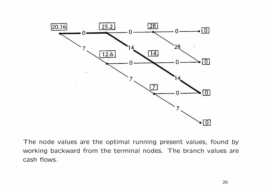
The node values are the optimal running present values, found by

working backward from the terminal nodes. The branch values are

cash flows.

26

Example – Complexico Mine

• If x is the amount of gold remaining in the mine at the beginning

of a year, the cost to extract z < x ounces of gold in that

year is $500z2/x. It is proportional to the product of amount z

extracted and the fraction z/x relative to amount x left behind.

• It is estimated that the current amount of gold remaining in

the mine is x0 = 50,000 ounces. The price of gold is $400/oz.

We are contemplating the purchase of a 10-year lease of the

Complexico mine. The interest rate is 10%. How much is this

lease worth?

27

Dynamic process – optimal operating plan

• We must determine how much gold to mine each year in order

to obtain the maximum present value.

• We index the time points by the number of years since the

beginning of the lease. The initial time is 0, the end of the first

year is 1, and so forth. The end of the lease is time 10. We also

assume that the cash flow from mining operations is obtained

at the beginning of the year.

• The optimal operating plan is exemplified by the reserve xn in

the mine at the beginning of the nth year. Then zn ounces are

extracted so that

xn+1 = xn − zn, n = 0,1, · · · ,9.

28

Solution for V9(x9)

• Only 1 year remains on the lease, so the value is obtained by

maximizing the profit for that year.

• If we extract z9 ounces, the revenue from the sale of the gold

will be gz9, where g is the price of gold, and the cost of mining

will be 500z29/x9.

• Hence, the optimal value of the mine at time 9 if x9 is the

remaining deposit level is

V9(x9) = maxz9

(gz9 − 500z29/x9), z9 ≤ x9.

29

We find the maximum by setting the derivative with respect to z9equal to zero. This yields (need to check z9 ≤ x9)

z9 = gx9/1,000.

We substitute this value in the formula for profit to find

V9(x9) =g2x9

1,000−

500g2x9

1,000 × 1,000=

g2x9

2,000.

We write this as V9(x9) = K9x9, where K9 = g2/2,000 is a constant.

Hence the value of the lease is directly proportional to how much

gold remains in the mine; the proportionality factor is K9.

Remark If gx9/1,000 > x9, then the maximum is attained at z9 =

x9.

30

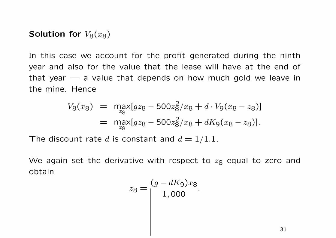
Solution for V8(x8)

In this case we account for the profit generated during the ninth

year and also for the value that the lease will have at the end of

that year — a value that depends on how much gold we leave in

the mine. Hence

V8(x8) = maxz8

[gz8 − 500z28/x8 + d · V9(x8 − z8)]

= maxz8

[gz8 − 500z28/x8 + dK9(x8 − z8)].

The discount rate d is constant and d = 1/1.1.

We again set the derivative with respect to z8 equal to zero and

obtain

z8 =(g − dK9)x8

1,000.

31

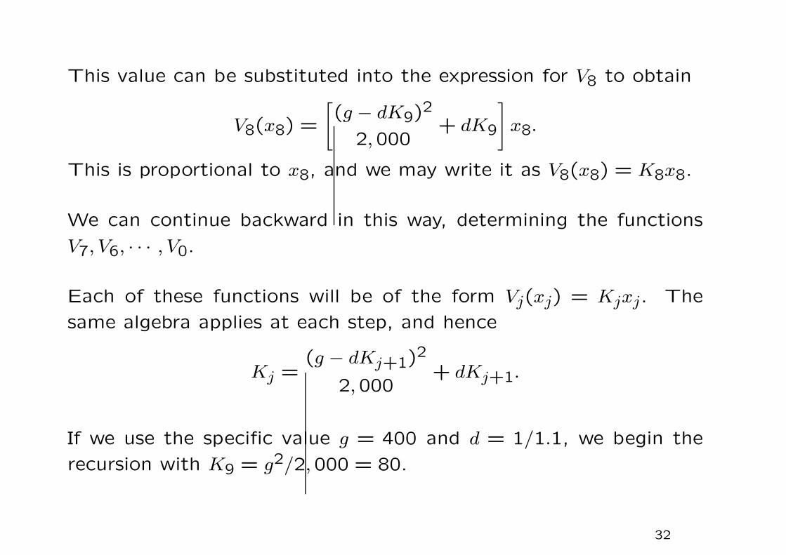
This value can be substituted into the expression for V8 to obtain

V8(x8) =

[

(g − dK9)2

2,000+ dK9

]

x8.

This is proportional to x8, and we may write it as V8(x8) = K8x8.

We can continue backward in this way, determining the functions

V7, V6, · · · , V0.

Each of these functions will be of the form Vj(xj) = Kjxj. The

same algebra applies at each step, and hence

Kj =(g − dKj+1)

2

2,000+ dKj+1.

If we use the specific value g = 400 and d = 1/1.1, we begin the

recursion with K9 = g2/2,000 = 80.

32

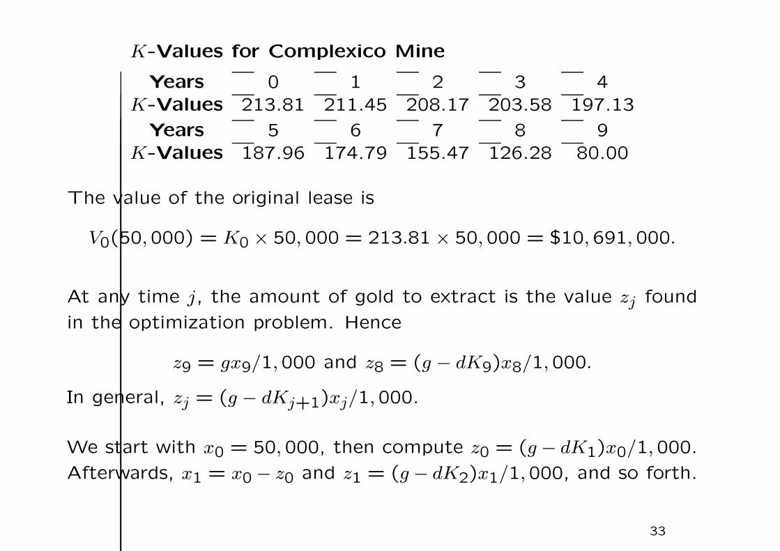
K-Values for Complexico Mine

Years 0 1 2 3 4

K-Values 213.81 211.45 208.17 203.58 197.13

Years 5 6 7 8 9

K-Values 187.96 174.79 155.47 126.28 80.00

The value of the original lease is

V0(50,000) = K0 × 50,000 = 213.81 × 50,000 = $10,691,000.

At any time j, the amount of gold to extract is the value zj found

in the optimization problem. Hence

z9 = gx9/1,000 and z8 = (g − dK9)x8/1,000.

In general, zj = (g − dKj+1)xj/1,000.

We start with x0 = 50,000, then compute z0 = (g − dK1)x0/1,000.

Afterwards, x1 = x0 − z0 and z1 = (g − dK2)x1/1,000, and so forth.

33

4.4 Harmony Theorem

Background

• There is a difference between the present value criterion for se-

lecting investment opportunities and the internal rate of return

criterion, and that it is strongly believed by theorists that the

present value criterion is the better of the two, provided that ac-

count is made for the entire cash flow stream of the investment

over all its period.

• But if you are asked to consider an investment of a fixed amount

of dollars, you probably would not evaluate this proposition in

terms of present value; you would more likely focus on potential

return.

34

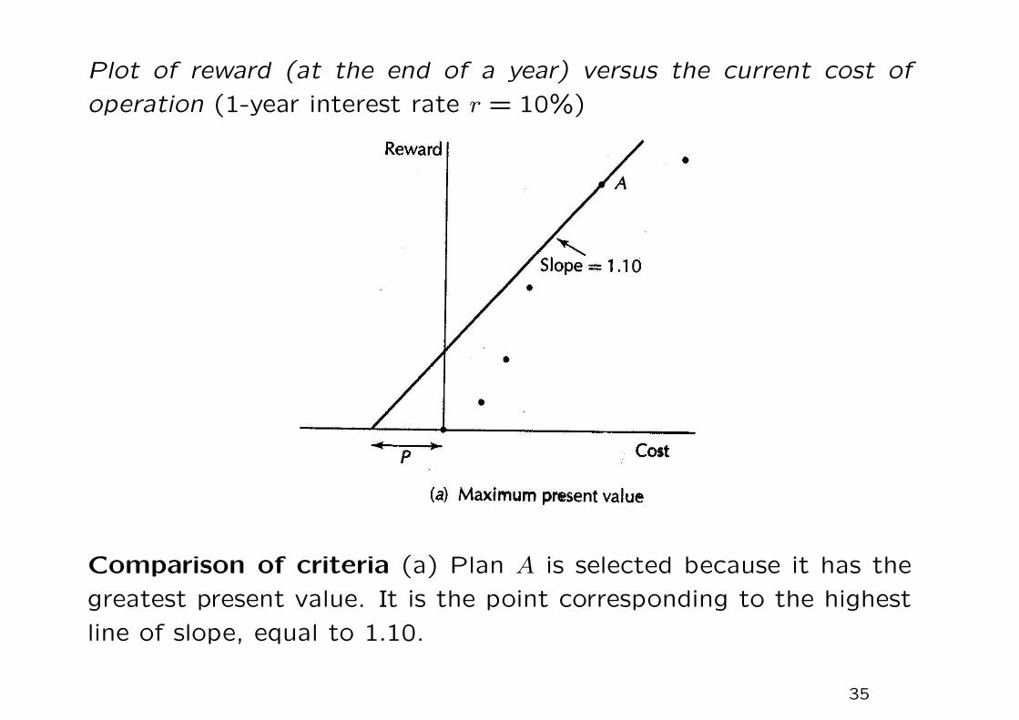
Plot of reward (at the end of a year) versus the current cost of

operation (1-year interest rate r = 10%)

Comparison of criteria (a) Plan A is selected because it has the

greatest present value. It is the point corresponding to the highest

line of slope, equal to 1.10.

35

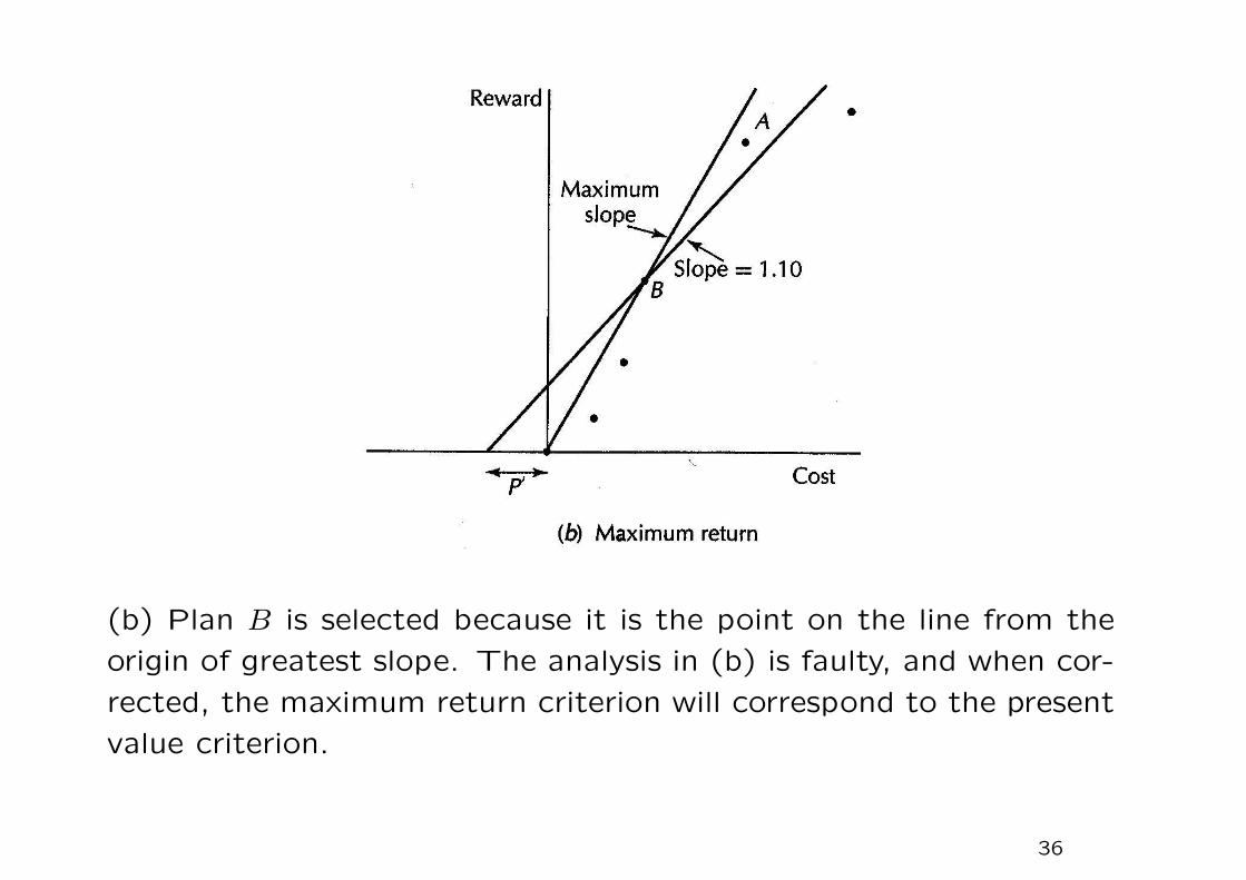
(b) Plan B is selected because it is the point on the line from the

origin of greatest slope. The analysis in (b) is faulty, and when cor-

rected, the maximum return criterion will correspond to the present

value criterion.

36

• If your friend sells you the venture, he will charge you an amount

P because that is what it would be worth to him if he kept

ownership. So if you decide to buy the venture, the total expense

of an operating plan is now P plus the actual operating cost.

• If you want to maximize your return, you will maximize

reward/(cost +P).

• You can find this new best operating plan by swinging a line

upward, pivoting around the point −P , reaching the operating

point with the greatest possible slope. That point will be point

A, the point that maximized the present value.

37

Harmony theorem Current owners of a venture should want to

operate the venture to maximize the present value of its cash flow

stream. Potential new owners, who must pay the full value of their

prospective share of the venture, will want the company to operate

in the same way, in order to maximize the return on their investment.

The harmony theorem is justification for operating a venture (such

as a company) in the way that maximizes the present value of the

cash flow stream it generates. Both current owners and potential

investors will agree on this policy.

38

4.5 Valuation of a firm

• Present value analysis is commonly used to estimate the value

of a firm. One such procedure is the dividend discount method,

where the value to a stockholder is assumed to be equal to

the present value of the stream of future dividend payments. If

dividends are assumed to grow at a rate g per year, a simple

formula gives the present value of the resulting stream.

39

Dividend Discount Models

The owner of a share of stock in a company can expect to receive

periodic dividends. Suppose that it is known that in year k, k =

1,2, · · · , a dividend of Dk will be received. If the interest rate (or

the discount rate) is fixed at r, it is reasonable to assign a value of

the firm to the stock holders as the present value of this dividend

stream; namely,

V0 =D1

1 + r+

D2

(1 + r)2+

D3

(1 + r)3+ · · · .

40

A popular way to specify dividends is to use the constant-growth

dividend model, where dividends grow at a constant rate g. In

particular, given D1 and the relation Dk+1 = (1+ g)Dk, the present

value of the stream is

V0 =D1

1 + r+

D1(1 + g)

(1 + r)2+

D1(1 + g)2

(1 + r)2+ · · · = D1

∞∑

k=1

(1 + g)k−1

(1 + r)k.

This summation is similar to that of an annuity. The summation

will have finite value only if the dividend growth rate is less than the

rate used for discounting; that is, if g < r. In that case we have the

explicit Gordon formula

V0 =D1

r − g.

41

The value of a firm’s stock increases if g increases, if the current

dividend D1 increases, or if the discount rate r decreases. All of

these properties are intuitively clear. If we project D1 from a current

dividend (already paid) of D0, we can rewrite the Gordon formula

by including the first-year’s growth.

Discounted growth formula Consider a dividend stream that grows

at a rate of g per period. Assign r > g as the discount rate per pe-

riod. Then the present value of the stream, starting one period

from the present, with the dividend D1, is

V0 =(1 + g)D0

r − g

where D0 is the current dividend.

To use the constant-growth dividend model one must estimate the

growth rate g and assign an appropriate value to the discount rate r.

Estimation of g can be based on the history of the firm’s dividends

and on future prospect.

42

Example (The XX Corporation) The XX Corporation has just

paid a dividend of $1.37M. The company is expected to grow at

10$ for the foreseeable future, and hence most analysts project a

similar growth in dividends. The discount rate used for this type of

company is 15%. What is the value of a share of stock in the XX

Corporation?

The total value of all shares is

V0 =1.37M × 1.10

0.15 − 0.10= $30,140,000.

Assume that there are 1 million shares outstanding. Each share is

worth $30.14 according to this analysis.

43

• The better method of firm evaluation bases the evaluation on

free cash flow, which is the amount of cash that can be taken

out of the firm while maintaining optimal operations and invest-

ment strategies. In idealized form, this method requires that

the present value of free cash flow be maximized with respect

to all possible management decisions, especially those related to

investment that produces earning growth.

• Valuation methods based on present value suffer the defect that

future cash flows are treated as if they were known with cer-

tainty, when in fact they are usually uncertain.

44

• Within the limitations of a deterministic approach, the best way

to value a firm is to determine the cash flow stream of maxi-

mum present value that can be taken out of the company and

distributed to the owners. The corresponding cash flow in any

year is termed that year’s free cash flow (FCF). Roughly, free

cash flow is the cash generated through operations minus the

investments necessary to sustain those operations and their an-

ticipated growth.

• It is difficult to obtain an accurate measure of the free cash flow.

First, it is necessary to assess the firm’s potential for generating

cash under various policies. Second, it is necessary to determine

the optimal rate of investment – the rate that will generate the

cash flow stream of maximum present value.

45

Suppose that a company has gross earning of Yn in year n and

decides to invest a portion u of this amount each year in order

to attain earnings growth. The growth rate is determined by the

function g(u), which is a property of the firm’s characteristics. On

a (simplified) accounting basis, depreciation is a fraction α of the

current capital account (α ≈ 0.10, for example). In this case the

capital Cn follows the formula

Cn+1 = (1 − α)Cn + uYn.

With these ideas we can set up a general income statement for a

firm, as shown in the following Table.

46

Free Cash Flow

Income statement

Before-tax cash flow from operations Yn

Depreciation αCn

Taxable income Yn − αCn

Taxes (34%) 0.34(Yn − αCn)After-fax income 0.66(Yn − αCn)After-tax cash flow(after-tax income plus depreciation) 0.66(Yn − αCn) + αCn

Sustaining investment uYn

Free cash flow 0.66(Yn − αCn) + αCn − uYn

Depreciation is assumed to be α times the account in the capital

account.

47

Example We can go further with the foregoing analysis and cal-

culate Yn and Cn in explicit form. Since

Yn+1 = [1 + g(u)]Yn,

it is easy to see that

Yn = [1 + g(u)]nY0.

Likewise, it can be shown that

Cn = (1 − α)nC0 + uY0

{

−(1 − α)n + [1 + g(u)]n

g(u) + α

}

.

If we ignore the two terms having (1 − α)n (since they will nearly

cancel) we have

Cn =uY0[1 + g(u)]n

g(u) + α.

48

Putting the expression for Yn and Cn in the bottom line of the Table,

we find the free cash flow at time n to be

FCF =

[

0.64 + 0.34αu

g(u) + α− u

]

[1 + g(u)]nY0.

This is a growing geometric series.

We can use the Gordon formula to calculate its present value at

interest rate r. This gives

PV =

[

0.66 + 0.34αu

g(u) + α− u

]

Y0

r − g(u). (A)

It is not easy to see by inspection what value of u would be best.

49

Example Assume that the XX Corporation has current earnings

of Y0 = $10 million, and the initial capital is C0 = $19.8 mil-

lion. The interest rate is r = 15%, the deprecation factor is

α = 0.10, and the relation between investment rate and growth

rate is g(u) = 0.12[1− e5(α−u)]. Notice that g(α) = 0, reflecting the

fact that an investment rate of α times earnings just keeps up with

the depreciation of capital.

Using eq. (A) we can find the value of the company of various

choices of the investment rate u.

• For example, for u = 0, no investment, the company will slowly

shrink, and the present value under that policy will be $29 mil-

lion.

• If u = 0.10, the company will just maintain its current level, and

the present value under that plan will be $39.6 million.

• Or if u = 0.5, the present value will be $52 million.

50

It is possible to maximize (A) (by trial and error or by a simple

optimization routine as is available in some spreadsheet packages).

The result is u = 37.7% and g(u) = 9.0%. The corresponding

present value is $58.3 million. This is the company value.

Question

Suppose that during the first year, the firm operates according to

this plan, investing 37.7% of its gross earnings in new capital. Sup-

pose also, for simplicity, that no dividends are paid that year. What

will be the value of the company after 1 year? Recall that during

this year, capital and earning expand by 9%. Would you guess that

the company value will increase by 9% as well?

51

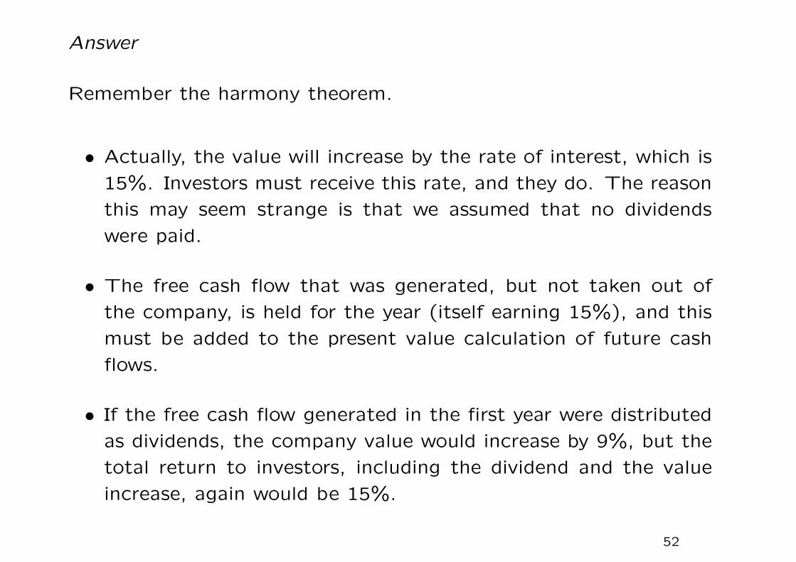
Answer

Remember the harmony theorem.

• Actually, the value will increase by the rate of interest, which is

15%. Investors must receive this rate, and they do. The reason

this may seem strange is that we assumed that no dividends

were paid.

• The free cash flow that was generated, but not taken out of

the company, is held for the year (itself earning 15%), and this

must be added to the present value calculation of future cash

flows.

• If the free cash flow generated in the first year were distributed

as dividends, the company value would increase by 9%, but the

total return to investors, including the dividend and the value

increase, again would be 15%.

52

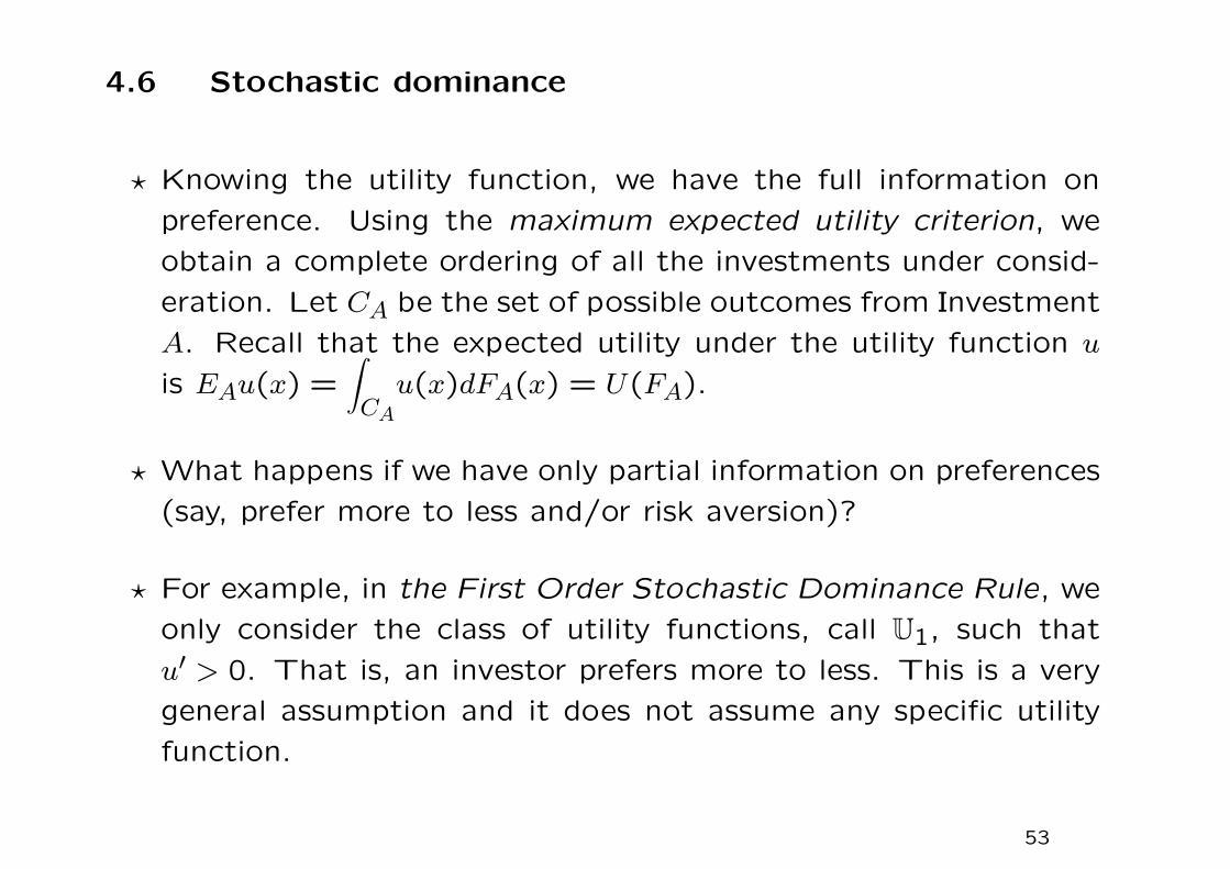
4.6 Stochastic dominance

⋆ Knowing the utility function, we have the full information on

preference. Using the maximum expected utility criterion, we

obtain a complete ordering of all the investments under consid-

eration. Let CA be the set of possible outcomes from Investment

A. Recall that the expected utility under the utility function u

is EAu(x) =

∫

CA

u(x)dFA(x) = U(FA).

⋆ What happens if we have only partial information on preferences

(say, prefer more to less and/or risk aversion)?

⋆ For example, in the First Order Stochastic Dominance Rule, we

only consider the class of utility functions, call U1, such that

u′ > 0. That is, an investor prefers more to less. This is a very

general assumption and it does not assume any specific utility

function.

53

• We define efficient sets under alternative assumptions about the

general characteristics of investors’ utility functions.

Dominance in U1

Investment A dominates Investment B in U1 if for all utility functions

such that u ∈ U1, EAu(x) ≥ EBu(x), or equivalently, U(FA) ≥ U(FB),

and for at least one utility function, there is a strict inequality.

Efficient set in U1 consists of investments that are not being domi-

nated

An investment is included in the efficient set if there is no other

investment that dominates it.

54

Inefficient set in U1

The inefficient set includes all inefficient investments. For an in-

efficient investment, it may be dominated by investments in the

efficient set or inefficient set. If it is not dominated by any invest-

ment in the inefficient set, then there is at least one investment in

the efficient set that dominates it. Otherwise, it should stay in the

efficient set.

The partition into efficient and inefficient sets depends on the choice

of the class of utility functions. In general, the smaller the efficient

set relative to the feasible set, the easier for the investor to make

decision.

55

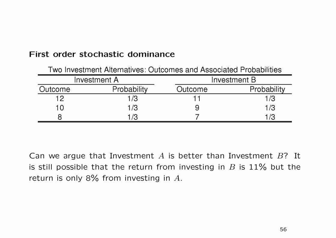
First order stochastic dominance

Can we argue that Investment A is better than Investment B? It

is still possible that the return from investing in B is 11% but the

return is only 8% from investing in A.

56

⋆ By looking at the cumulative probability distribution, we observe

that for all returns and the odds of obtaining that return or less,

B consistently has a higher or same value.

57

58

Recall that for each investment choice, there is an induced probabil-

ity distribution on C (the set of all consequences). To compare two

choices, we examine their corresponding probability distribution.

Definition

A probability distribution F dominates another probability distribu-

tion G according to the first-order stochastic dominance when F

and G satisfy

F(x) ≤ G(x) for all x ∈ C.

Lemma

F dominates G by FSD if and only if∫

Cu(x) dF(x) ≥

∫

Cu(x) dG(x)

for all strictly increasing utility u(x).

59

Proof

Let a and b be the smallest and largest values that F and G can

take on. Consider∫ b

au(x) d[F(x)−G(x)] = u(x)[F(x) − G(x)]ba︸ ︷︷ ︸

zero since F (a) = G(a) = 0and F (b) = G(b) = 1

−

∫ b

au′(x)[F(x)−G(x)] dx

∫

Cu(x) dF(x) ≥

∫

Cu(x) dG(x) ⇔ −

∫ b

au′(x)[F(x) − G(x)] dx ≥ 0.

Thus, for u′(x) > 0,

F(x) ≤ G(x) ⇐⇒

∫

Cu(x) dF(x) ≥

∫

Cu(x) dG(x).

60

Second order stochastic dominance

If both investments turn out the worst, the investor obtains 6%

from A and only 5% from B. If the second worst return occurs, the

investor obtains 8% from A rather than 9% from B. If he is risk

averse, then he should be willing to lose 1% in return at a higher

level of return in order to obtain an extra 1% at a lower return level.

If risk aversion is assumed, then A is preferred to B.

61

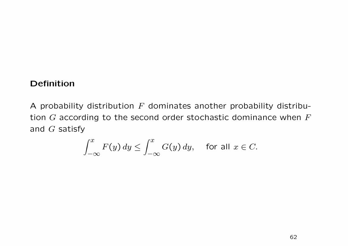
Definition

A probability distribution F dominates another probability distribu-

tion G according to the second order stochastic dominance when F

and G satisfy∫ x

−∞F(y) dy ≤

∫ x

−∞G(y) dy, for all x ∈ C.

62

According to SSD, A is preferred over B since the sum of cumulative

probability for A is always less than or equal to that for B.

63

Theorem

If F dominates G by SSD, then∫

Cu(x) dF(x) ≥

∫

Cu(x) dG(x)

for all increasing and concave utility u(x).

Proof∫ b

au(x) d[F(x) − G(x)] = −

∫ b

au′(x)[F(x) − G(x)] dx

= −u′(x)∫ x

a[F(y) − G(y)] dy

∣∣∣∣∣

b

a

+

∫ b

au′′(x)

∫ x

a[F(y) − G(y)] dydx

= −u′(b)∫ b

a[F(y) − G(y)] dy

+

∫ b

au′′(x)

∫ x

a[F(y) − G(y)] dydx.

Given that u′(b) > 0 and u′′(x) < 0,∫

Cu(x) dF(x) ≥

∫

Cu(x) dG(x) if

∫ x

a[F(y) − G(y)] dy ≤ 0,∀x.

64

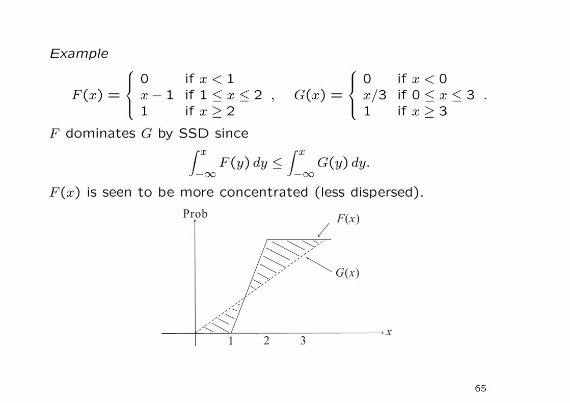
Example

F(x) =

0 if x < 1x − 1 if 1 ≤ x ≤ 21 if x ≥ 2

, G(x) =

0 if x < 0x/3 if 0 ≤ x ≤ 31 if x ≥ 3

.

F dominates G by SSD since∫ x

−∞F(y) dy ≤

∫ x

−∞G(y) dy.

F(x) is seen to be more concentrated (less dispersed).

65

Sufficient rules and necessary rules for second order stochastic

dominance

Sufficient rule 1: FSD rule is sufficient for SSD

Proof : If F dominates G by FSD, then F(x) ≤ G(x), ∀x.

This implies

∫ x

a[G(y) − F(y)] dy ≥ 0.

Remark

Since SSD rule requires risk aversion in addition to FSD rule, some

elements in the inefficient set according to FSD may not stay again

in the inefficient set of SSD. The efficient set according to SSD is

larger than that of FSD.

66

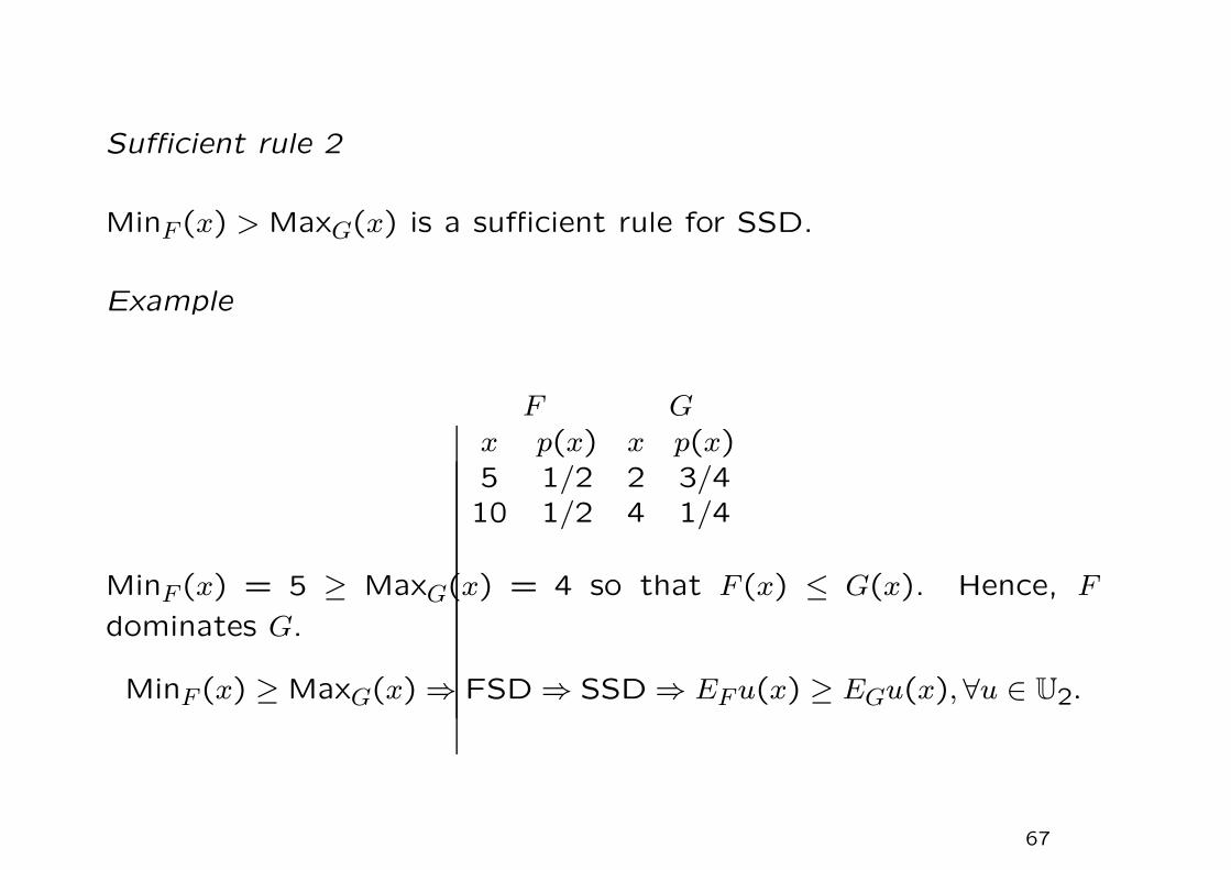
Sufficient rule 2

MinF (x) > MaxG(x) is a sufficient rule for SSD.

Example

F Gx p(x) x p(x)5 1/2 2 3/410 1/2 4 1/4

MinF (x) = 5 ≥ MaxG(x) = 4 so that F(x) ≤ G(x). Hence, F

dominates G.

MinF (x) ≥ MaxG(x) ⇒ FSD ⇒ SSD ⇒ EFu(x) ≥ EGu(x),∀u ∈ U2.

67

Xgeo(F ) ≥ Xgeo(G) is a necessary condition for dominance of F over G by SSD.

Given a risky project with the distribution (xi, pi), i = 1, · · · , n, the

geometric mean, Xgeo, is defined as

Xgeo = xp11 · · ·xpn

n =n∏

i=1

xpii , xi ≥ 0.

Taking logarithm on both sides

lnXgeo = Σpi ln xi = E[lnX].

Suppose F dominates G by SSD, we have

EFu(x) ≥ EGu(x), ∀u ∈ U2.

Since lnx = u(x) ∈ U2,

EF lnx = lnF Xgeo ≥ EG lnx = lnG Xgeo;

we obtain lnXgeo(F) ≥ lnXgeo(G). Since the logarithm function is

an increasing function, we deduce Xgeo(F) ≥ Xgeo(G). Therefore,

F dominates G by SSD ⇒ Xgeo(F) ≥ Xgeo(G).

68

Necessary rule 2 (left-tail rule)

Suppose F dominates G by SSD, then

MinF (x) ≥ MinG(x),

that is, the left tail of G must be “thicker”.

Proof by contradiction:

Suppose MinF (x) < MinG(x), and write xk = MinF (x). At xk, G will

still be zero but F will be positive. Observe that∫ xk

−∞[G(y) − F(y)] dy =

∫ xk

−∞[0 − F(y)] dy < 0,

implying F is not dominated by G by SSD. Hence, if F dominates

G, then MinF (x) ≥ MinG(x).

69