4 marriage and divorce since world war ii: analyzing the … the fraction of the population that is...
TRANSCRIPT
4
Marriage and Divorce since World War II:Analyzing the Role of Technological Progresson the Formation of Households
Jeremy Greenwood, University of Pennsylvania and NBER
Nezih Guner, Universidad Carlos III de Madrid, CEPR, and IZA
I. Introduction
Consider the following two facts that have helped reshape U.S. house-holds over the last 50 years:
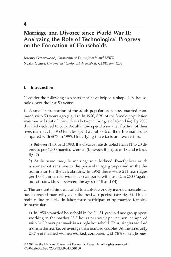
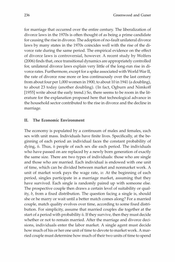
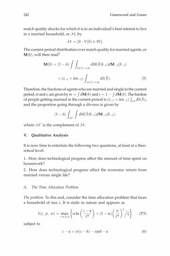
1. A smaller proportion of the adult population is now married com-pared with 50 years ago (fig. 1).1 In 1950, 82% of the female populationwas married (out of nonwidows between the ages of 18 and 64). By 2000this had declined to 62%. Adults now spend a smaller fraction of theirlives married. In 1950 females spent about 88% of their life married ascompared with 60% in 1995. Underlying these facts are two factors:
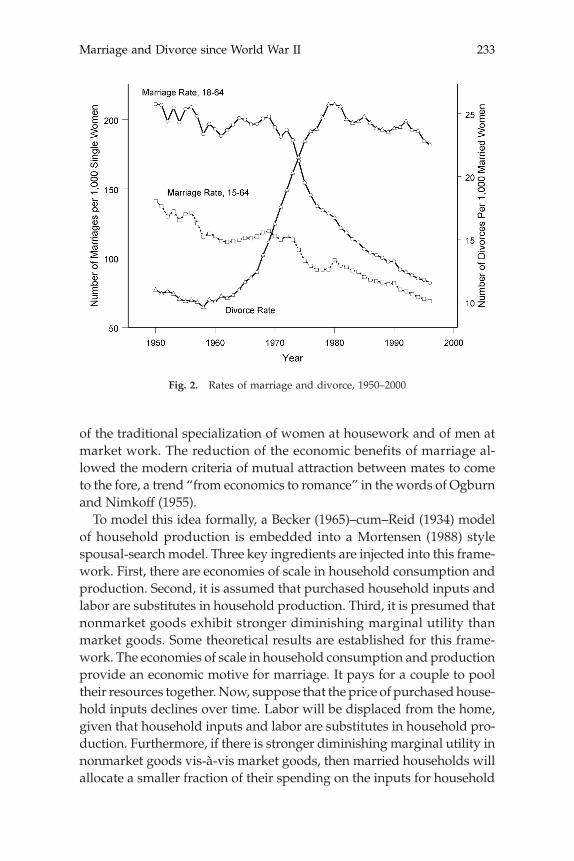
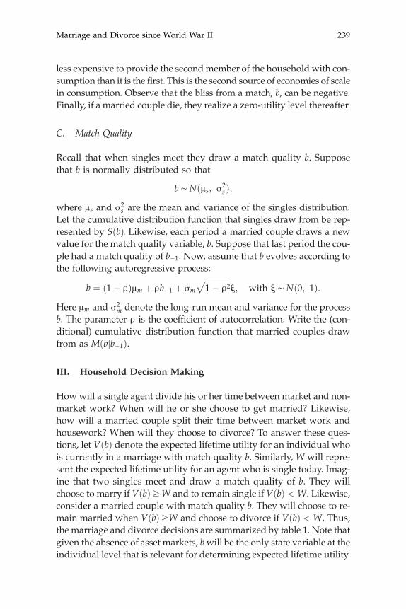
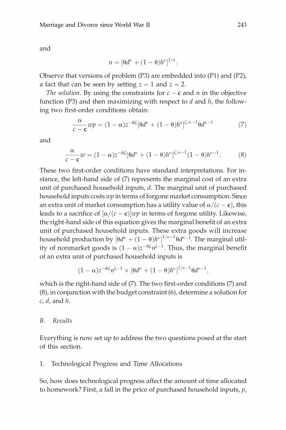
a) Between 1950 and 1990, the divorce rate doubled from 11 to 23 di-vorces per 1,000 married women (between the ages of 18 and 64; seefig. 2).
b) At the same time, the marriage rate declined. Exactly how muchis somewhat sensitive to the particular age group used in the de-nominator for the calculations. In 1950 there were 211 marriagesper 1,000 unmarried women as compared with just 82 in 2000 (again,out of nonwidows between the ages of 18 and 64).
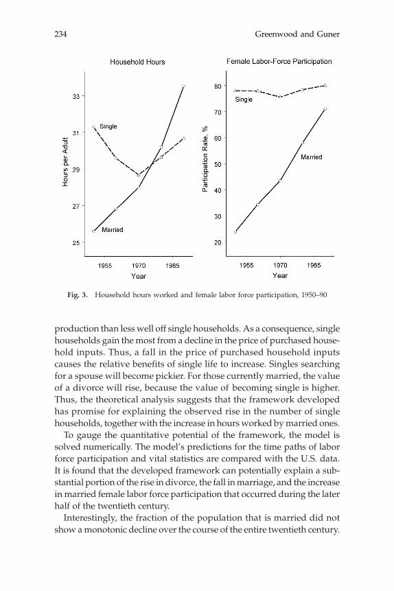
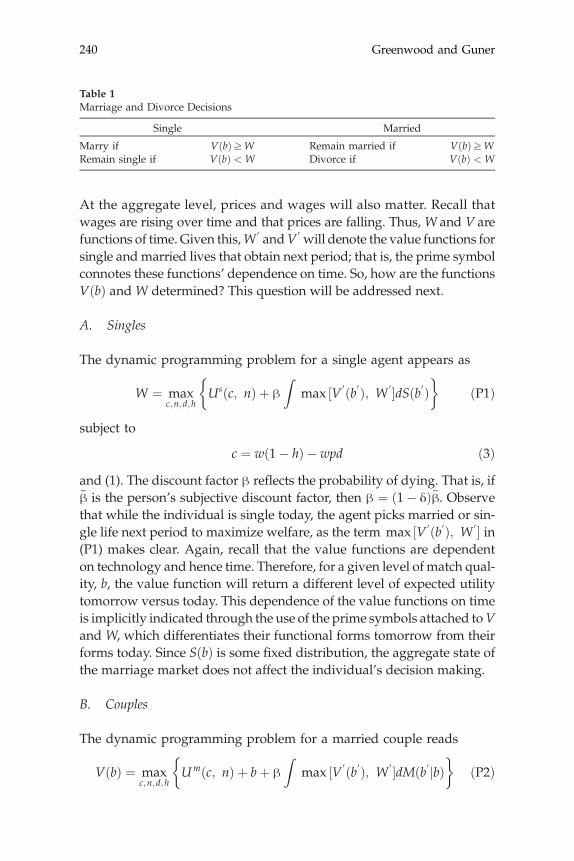
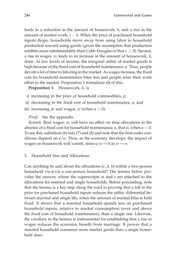
2. The amount of time allocated to market work by married householdshas increased markedly over the postwar period (see fig. 3). This ismainly due to a rise in labor force participation by married females.In particular:
a) In 1950 amarried household in the 24–54‐year‐old age group spentworking in the market 25.5 hours per week per person, comparedwith 31.3 hours per week in a single household. Thus, singles workedmore in themarket on average thanmarried couples. At the time, only23.7% of married women worked, compared with 78% of single ones.
© 2009 by the National Bureau of Economic Research. All rights reserved.978‐0‐226‐00204‐0/2009/2008‐0401$10.00

Greenwood and Guner232
b) By the year 1990 labor effort expendedper person bymarried house-holds had risen to 33.5 hours per week. This exceeded the 30.6 hoursspent by a single household. Almost as many married females wereparticipating in the labor market (71%) as single ones (80%).
What economic factors can explain these facts? The idea here is thattechnological progress played a major role in inducing these changes.2
Two hundred years ago the United States was largely a rural economy.The household was the basic production unit, with the family produc-ing a large fraction of what it consumed. At the time, most marriageswere arranged by the parents of young adults. Key considerations werewhether or not the potential groom would be a good provider and thebride a good housekeeper.3 Over time more and more household goodsand services could be purchased outside the home, such as packagedfoods and ready‐made clothes. Additionally capital goods, ranging fromwashing machines to microwave ovens, were brought into the home,greatly reducing the time needed to maintain a household. This hadtwo effects. First, it allowed all adults, bothmarried and single, to devotemore time tomarket activities and less to household production. Second,it lowered the economic incentives to get married by reducing the benefits
Fig. 1. Marriage, 1950–2000
Marriage and Divorce since World War II 233
of the traditional specialization of women at housework and of men atmarket work. The reduction of the economic benefits of marriage al-lowed the modern criteria of mutual attraction between mates to cometo the fore, a trend “from economics to romance” in the words of Ogburnand Nimkoff (1955).To model this idea formally, a Becker (1965)–cum–Reid (1934) model
of household production is embedded into a Mortensen (1988) stylespousal‐searchmodel. Three key ingredients are injected into this frame-work. First, there are economies of scale in household consumption andproduction. Second, it is assumed that purchased household inputs andlabor are substitutes in household production. Third, it is presumed thatnonmarket goods exhibit stronger diminishing marginal utility thanmarket goods. Some theoretical results are established for this frame-work. The economies of scale in household consumption and productionprovide an economic motive for marriage. It pays for a couple to pooltheir resources together.Now, suppose that the price of purchased house-hold inputs declines over time. Labor will be displaced from the home,given that household inputs and labor are substitutes in household pro-duction. Furthermore, if there is stronger diminishing marginal utility innonmarket goods vis‐à‐vis market goods, then married households willallocate a smaller fraction of their spending on the inputs for household
Fig. 2. Rates of marriage and divorce, 1950–2000
Greenwood and Guner234
production than less well off single households. As a consequence, singlehouseholds gain themost from a decline in the price of purchased house-hold inputs. Thus, a fall in the price of purchased household inputscauses the relative benefits of single life to increase. Singles searchingfor a spouse will become pickier. For those currently married, the valueof a divorce will rise, because the value of becoming single is higher.Thus, the theoretical analysis suggests that the framework developedhas promise for explaining the observed rise in the number of singlehouseholds, together with the increase in hoursworked bymarried ones.To gauge the quantitative potential of the framework, the model is
solved numerically. The model’s predictions for the time paths of laborforce participation and vital statistics are compared with the U.S. data.It is found that the developed framework can potentially explain a sub-stantial portion of the rise in divorce, the fall inmarriage, and the increasein married female labor force participation that occurred during the laterhalf of the twentieth century.Interestingly, the fraction of the population that is married did not
show amonotonic decline over the course of the entire twentieth century.
Fig. 3. Household hours worked and female labor force participation, 1950–90
Marriage and Divorce since World War II 235
It actually increased during the baby boom years. This resulted in ahump‐shaped time path for marriage during the last century. Is this ob-servation congruent with theory presented here? The answer is yes. It isdemonstrated that a simple extension of the basic framework has the po-tential to address this fact. It does so by linking a young adult’s decisionto leave home and search for a mate with technological progress in thehousehold sector. The extension can explain the drop in the number ofyoung adults living with their parents over the last 100 years.A prediction of the framework is that household size should decline
when the price of purchased household inputs falls. The relationshipbetween household size and the price of household appliances is exam-ined econometrically for a small cross section ofWestern countries. A pos-itive association is found, in accordancewith the theory ’s prediction. Thisfinding complements recent work by Cavalcanti and Tavares (2008), whoreport that female labor supply is negatively associated with the price ofhousehold appliances in a panel of countries. Algan and Cahuc (2007)also find that it is related to the labor supply of younger and older(non‐prime‐age) workers, but in a way that interacts with cultural differ-ences across countries. Likewise, Coen‐Pirani, Leon, and Lugauer (2008)conclude, using U.S. Census micro data, that a significant portion of therise in married female labor force participation during the 1960s can beattributed to the diffusion of household appliances.It needs to be stated up‐front that the goal of the analysis is not to
simulate an all‐inclusive model of household formation and labor forceparticipation. Rather, the idea here is to see whether or not the simplemechanisms put forth have the potential quantitative power to explainthe postwar observations on household formation and labor force par-ticipation. This is done without regard to the many other possible ex-planations for the same set of facts—some of which could be embeddedinto a more general version of the developed framework. Theory, by itsessence, is a process of abstraction. Therefore, some factors that may beimportant for understanding the phenomena under study have beendeliberately left out of the analysis, for purposes of both clarity and trac-tability; see Stevenson andWolfers (2007) for a recent survey onmarriageand divorce.For example, the tremendous amount of technological progress in
contraception that occurred over the last century greatly reduced the riskof out‐of‐wedlock sexual relationships. It seems very likely that this pro-vided impetus for the fall inmarriage and the rise in divorce that occurredsinceWorldWar II. It might be hard for a theory based on improvementsin contraception alone, however, to explain the hump‐shaped time path
Greenwood and Guner236
for marriage that occurred over the entire century. The liberalization ofdivorce laws in the 1970s is often thought of as being a prime candidatefor causing the rise in divorce. The adoption of no‐fault unilateral divorcelaws by many states in the 1970s coincides well with the rise of the di-vorce rate during the same period. The empirical evidence on the effectof divorce laws is controversial, however. A recent study by Wolfers(2006) finds that, once transitional dynamics are appropriately controlledfor, unilateral divorce laws explain very little of the long‐run rise in di-vorce rates. Furthermore, except for a spike associatedwithWorldWar II,the rate of divorce rose more or less continuously over the last centuryfromabout four per 1,000women in 1900, to about 10 in 1941 (a doubling),to about 23 today (another doubling). ( In fact, Ogburn and Nimkoff[1955] write about the early trend.) So, there seems to be room in the lit-erature for the explanation proposed here that technological advance inthe household sector contributed to the rise in divorce and the decline inmarriage.
II. The Economic Environment
The economy is populated by a continuum of males and females, eachsex with unit mass. Individuals have finite lives. Specifically, at the be-ginning of each period an individual faces the constant probability ofdying, δ. Thus, δ people of each sex die each period. The individualswho have passed on are replaced by a newly born generation of exactlythe same size. There are two types of individuals: those who are singleand those who are married. Each individual is endowed with one unitof time, which can be divided between market and nonmarket work. Aunit of market work pays the wage rate, w. At the beginning of eachperiod, singles participate in a marriage market, assuming that theyhave survived. Each single is randomly paired up with someone else.The prospective couple then draws a certain level of suitability or qual-ity, b, from a fixed distribution. The question facing a single is, shouldshe or he marry or wait until a better match comes along? For a marriedcouple, match quality evolves over time, according to some fixed distri-bution. For simplicity, assume that married couples die together at thestart of a periodwith probability δ. If they survive, then theymust decidewhether or not to remain married. After the marriage and divorce deci-sions, individuals enter the labor market. A single agent must decidehowmuch of his or her one unit of time to devote tomarket work. Amar-ried couplemust determine howmuch of their two units of time to spend

Marriage and Divorce since World War II 237
in the labor force. For simplicity, it is assumed that there arenoassetmarkets.Hence, there is no borrowing or lending, and so forth, in the economy.Finally, as will become clear, there are no matching externalities presentin the model. The aggregate state of the marriage market will not influ-ence a household’s decision making.
A. Production
Start with production. Two types of goods are produced, market andnonmarket ones.
1. Household Production
Suppose that nonmarket goods, n, are produced in line with the follow-ing household production function:
n ¼ ½θdκ þ ð1� θÞhκ�1=κ for 0 < κ < 1; ð1Þwhere d denotes purchases of household inputs, and h is the amount oftime spent on housework. Let purchased household inputs sell at pricep, measured in terms of time. The idea here is that over time pwill drop.Specifically, let p fall monotonically to some lower bound p > 0. In re-sponse households will substitute out of using labor toward using morepurchased inputs. Note that it has been assumed that purchased inputsand time are more substitutable in production than Cobb‐Douglas, thatis, κ > 0. Hence, as p declines, household production will become moregoods intensive and less labor intensive. Examples of laborsaving house-hold inputs abound: disposable diapers, frozen foods, microwave ovens,washing machines, and Tupperware.
2. Market Production
Market goods are produced in line with the constant‐returns‐to‐scaleproduction technology
y ¼ wl; ð2Þwhere y is aggregate output and l is aggregate employment. Given thelinear form for the aggregate production function, w will represent thereal wage rate in equilibrium. Real wages will grow over time. In par-ticular, suppose that w increases monotonically to some finite upperbound w. There is no physical or, as mentioned, financial capital in the

Greenwood and Guner238
economy. Market output y is used for two purposes, namely, direct con-sumption and as an input into household production. Specifically, oneunit of output can be used to produce one unit of final consumptionor 1=ðwpÞ units of household inputs. Thus, the economy’s resource con-straint reads
cþ wpd ¼ y;
where c and d represent aggregate consumption and purchases of house-hold inputs, respectively.
B. Tastes
Singles. Let the momentary utility function for a single read
Usðc; nÞ ¼ α ln ðc� cÞ þ ð1� αÞnζ=ζ; with 0 < α < 1; ζ < 0≤ c:
Here c and n denote the person’s consumption of market and nonmarketgoods, respectively. The constant c is a fixed cost associated with main-taining a household. This represents the first of two sources of scaleeconomies in household consumption. Note that the utility functionfor nonmarket goods is more concave than the ln function (i.e., ζ < 0).The importance of this restriction will become clear as the theory is de-veloped. This constraint is not imposed in the quantitative analysis.Therefore, the data will speak to the sign and magnitude of ζ. If a singledies, he realizes a utility level of zero in the afterlife, an innocuous nor-malization. Leisure has been excluded from the tastes. This is in line withthe Beckerian (1965, 504) theory of household production since “althoughthe social philosopher might have to define precisely the concept of lei-sure, the economist can reach all his traditional results aswell asmanymorewithout introducing it at all.”The idea here is that often all one cares about istime spent in themarket versus at home, and the above frameworkwill cap-ture this through the production side of things. Additionally, observe thata separable form for the utility function is chosen, as is conventional inmacroeconomics. This minimizes the role placed on home production.Married individuals. Tastes for a married individual are given by
Umðc; nÞ þ b ¼α ln ½ðc� cÞ=2ϕ� þ ð1� αÞðn=2ϕÞζ=ζþ b; with 0 <ϕ < 1;
where c and n represent the household’s consumption of market andnonmarket goods. To determine an individual’s consumption, c� c andn are divided by the household equivalence scale, 2ϕ, to get consumptionper member, ðc� cÞ=2ϕ and n=2ϕ. Since 0 < ϕ < 1, this implies that it is
Marriage and Divorce since World War II 239
less expensive to provide the secondmember of the household with con-sumption than it is the first. This is the second source of economies of scalein consumption. Observe that the bliss from a match, b, can be negative.Finally, if a married couple die, they realize a zero‐utility level thereafter.
C. Match Quality
Recall that when singles meet they draw a match quality b. Supposethat b is normally distributed so that
b∼Nðμs; σ2s Þ;
where μs and σ2s are the mean and variance of the singles distribution.
Let the cumulative distribution function that singles draw from be rep-resented by SðbÞ. Likewise, each period a married couple draws a newvalue for the match quality variable, b. Suppose that last period the cou-ple had a match quality of b�1. Now, assume that b evolves according tothe following autoregressive process:
b ¼ ð1� ρÞμm þ ρb�1 þ σm
ffiffiffiffiffiffiffiffiffiffiffiffiffi1� ρ2
pξ; with ξ∼Nð0; 1Þ:
Here μm and σ2m denote the long‐run mean and variance for the process
b. The parameter ρ is the coefficient of autocorrelation. Write the (con-ditional) cumulative distribution function that married couples drawfrom as Mðbjb�1Þ.
III. Household Decision Making
Howwill a single agent divide his or her time between market and non-market work? When will he or she choose to get married? Likewise,how will a married couple split their time between market work andhousework? When will they choose to divorce? To answer these ques-tions, let VðbÞ denote the expected lifetime utility for an individual whois currently in a marriage with match quality b. Similarly, W will repre-sent the expected lifetime utility for an agent who is single today. Imag-ine that two singles meet and draw a match quality of b. They willchoose to marry if VðbÞ≥W and to remain single if VðbÞ < W. Likewise,consider a married couple with match quality b. They will choose to re-main married when VðbÞ≥W and choose to divorce if VðbÞ < W. Thus,the marriage and divorce decisions are summarized by table 1. Note thatgiven the absence of asset markets, bwill be the only state variable at theindividual level that is relevant for determining expected lifetime utility.
Greenwood and Guner240
At the aggregate level, prices and wages will also matter. Recall thatwages are rising over time and that prices are falling. Thus, W and V arefunctions of time. Given this,W′ andV′ will denote the value functions forsingle and married lives that obtain next period; that is, the prime symbolconnotes these functions’ dependence on time. So, how are the functionsVðbÞ and W determined? This question will be addressed next.
A. Singles
The dynamic programming problem for a single agent appears as
W ¼ maxc;n;d;h
�Usðc; nÞ þ β
Zmax ½V′ðb′Þ; W′�dSðb′Þ
�ðP1Þ
subject to
c ¼ wð1� hÞ � wpd ð3Þand (1). The discount factor β reflects the probability of dying. That is, ifβ~is the person’s subjective discount factor, then β ¼ ð1� δÞβ~. Observe
that while the individual is single today, the agent picks married or sin-gle life next period to maximize welfare, as the term max ½V′ðb′Þ; W′� in(P1) makes clear. Again, recall that the value functions are dependenton technology and hence time. Therefore, for a given level of match qual-ity, b, the value function will return a different level of expected utilitytomorrow versus today. This dependence of the value functions on timeis implicitly indicated through the use of the prime symbols attached toVand W, which differentiates their functional forms tomorrow from theirforms today. Since SðbÞ is some fixed distribution, the aggregate state ofthe marriage market does not affect the individual’s decision making.
B. Couples
The dynamic programming problem for a married couple reads
VðbÞ ¼ maxc;n;d;h
�Umðc; nÞ þ bþ β
Zmax ½V′ðb′Þ; W′�dMðb′jbÞ
�ðP2Þ
Table 1Marriage and Divorce Decisions
Single
MarriedMarry if
VðbÞ≥W Remain married if VðbÞ≥W Remain single if VðbÞ < W Divorce if VðbÞ < W
Marriage and Divorce since World War II 241
subject to
c ¼ wð2� hÞ � wpd ð4Þand (1). Problem (P2) is similar in structure to problem (P1) with threedifferences: (i) the utility function for married agents differs from thatfor single agents because of scale effects in household consumption;(ii) a married couple realizes bliss from marriage, and this is autocorre-lated over time; and (iii) the couple has two units of time to allocate be-tweenmarket and nonmarket work. Again, note that while an individualis married today, the agent chooses married or single life next period tomaximize welfare. Finally, the aggregate state of the marriage marketdoes not impinge on the couple’s decision making because Mðb′jbÞ is afixed distribution.
IV. Equilibrium
Formulating an equilibrium to the above economy is surprisingly simple.First, given the linear market production function (2), there is no need todetermine the equilibrium wage, w. Second, since there are no financialmarkets, there is no interaction between households other than throughthe marriage market. As far as consumption and production are con-cerned, each household is an island unto itself. Also, there are no match-ing externalities in the model. Each single is matched with a potentialmate each period. This pair then draws a quality for the match, b, fromthe fixed distribution SðbÞ. Likewise, the b for a couple evolves accordingto the fixed distribution Mðb′jbÞ. Hence, household decision making isnot influenced by the aggregate state of the marriage market. Therefore,characterizing an equilibrium for the economy amounts to solving theprogramming problems (P1) and (P2). Thus, it is easy to establish thatan equilibrium for the above economy both exists and is unique.Vital statistics. Computing vital statistics for the economy is a rela-
tively straightforward task. Suppose that the economy exits the previousperiodwith the (nonnormalized) distributionM�1ðb�1Þ overmatch qual-ity formarried agents of a particular sex. The fractions of agents (of a par-ticular sex) who were married and single last period, m�1 and s�1, aretherefore given by m�1 ¼
RdM�1ðb�1Þ and s�1 ¼ 1� R
dM�1ðb�1Þ. Now,at the beginning of the current period the fraction δ of the populace dies.These people are replaced by newly born single agents. All agents willthen take a draw, b, for theirmatch quality. After this, theywillmake theirmarriage and divorce decisions in line with table 1. Define the set of
Greenwood and Guner242
match quality shocks for which it is in an individual’s best interest to livein a married household, or M, by
M ¼ fb : VðbÞ≥Wg:The current‐period distribution overmatch quality formarried agents, orMðbÞ, will then read4
MðbÞ ¼ ð1� δÞZ Z
M∩½�∞;b�dMðb~ jb�1ÞdM�1ðb�1Þ
þ ðs�1 þ δm�1ÞZM∩½�∞;b�
dSðb~ Þ: ð5Þ
Therefore, the fractions of agentswho aremarried and single in the currentperiod,m and s, are givenbym ¼ R
dMðbÞ and s ¼ 1� RdMðbÞ. The fraction
of people getting married in the current period is ðs�1 þ δm�1ÞRM dSðb~ Þ,
and the proportion going through a divorce is given by
ð1� δÞZMc
ZdMðb~ jb�1ÞdM�1ðb�1Þ;
where Mc is the complement of M .
V. Qualitative Analysis
It is now time to entertain the following two questions, at least at a theo-retical level:
1. How does technological progress affect the amount of time spent onhousework?
2. How does technological progress affect the economic return frommarried versus single life?
A. The Time Allocation Problem
The problem. To this end, consider the time allocation problem that facesa household of size z. It is static in nature and appears as
Iðz; p; wÞ ¼ maxc;n;h;d
�α ln
�c� czϕ
�þ ð1� αÞ
�nzϕ
�ζ.ζ�
ðP3Þ
subject to
c� c ¼ wðz� hÞ � wpd� c ð6Þ
Marriage and Divorce since World War II 243
and
n ¼ ½θdκ þ ð1� θÞhκ�1=κ:Observe that versions of problem (P3) are embedded into (P1) and (P2),a fact that can be seen by setting z ¼ 1 and z ¼ 2.The solution. By using the constraints for c� c and n in the objective
function (P3) and then maximizing with respect to d and h, the follow-ing two first‐order conditions obtain:
αc� c
wp ¼ ð1� αÞz�ϕζ½θdκ þ ð1� θÞhκ�ζ=κ�1θdκ�1 ð7Þ
and
αc� c
w ¼ ð1� αÞz�ϕζ½θdκ þ ð1� θÞhκ�ζ=κ�1ð1� θÞhκ�1: ð8Þ
These two first‐order conditions have standard interpretations. For in-stance, the left‐hand side of (7) represents the marginal cost of an extraunit of purchased household inputs, d. The marginal unit of purchasedhousehold inputs costswp in terms of forgonemarket consumption. Sincean extra unit of market consumption has a utility value of α=ðc� cÞ, thisleads to a sacrifice of ½α=ðc� cÞ�wp in terms of forgone utility. Likewise,the right‐hand side of this equation gives the marginal benefit of an extraunit of purchased household inputs. These extra goods will increasehousehold production by ½θdκ þ ð1� θÞhκ�1=κ�1θdκ�1. The marginal util-ity of nonmarket goods is ð1� αÞz�ϕζnζ�1. Thus, the marginal benefitof an extra unit of purchased household inputs is
ð1� αÞz�ϕζnζ�1 � ½θdκ þ ð1� θÞhκ�1=κ�1θdκ�1;
which is the right‐hand side of (7). The two first‐order conditions (7) and(8), in conjunctionwith the budget constraint (6), determine a solution forc, d, and h.
B. Results
Everything is now set up to address the two questions posed at the startof this section.
1. Technological Progress and Time Allocations
So, how does technological progress affect the amount of time allocatedto homework? First, a fall in the price of purchased household inputs, p,
Greenwood and Guner244
leads to a reduction in the amount of housework, h, and a rise in theamount of market work, z� h. When the price of purchased householdinputs drops, households move away from using labor in householdproduction toward using goods (given the assumption that productionexhibits more substitutability than Cobb‐Douglas or that κ > 0). Second,a rise in wages, w, leads to an increase in the amount of housework, h,done. At low levels of income, the marginal utility of market goods ishigh because of the fixed cost of household maintenance, c. Thus, peopledevote a lot of time to laboring in themarket. Aswages increase, the fixedcost for household maintenance bites less and people relax their workeffort in the market. Proposition 1 formalizes all of this.Proposition 1. Housework, h, is
i) increasing in the price of household commodities, p;
ii) decreasing in the fixed cost of household maintenance, c; and
iii) increasing in real wages, w (when c > 0).
Proof. See the appendix.Remark. Real wages, w, will have no effect on time allocations in the
absence of a fixed cost for household maintenance, c, that is, when c ¼ 0.To see this, substitute (6) into (7) and (8) and note that the first‐order con-ditions depend on c=w. Thus, as the economy develops, the impact ofwages on housework will vanish, since c=w→ 0 as w→∞.
2. Household Size and Allocations
Can anything be said about the allocations (c, d, h) within a two‐personhousehold vis‐à‐vis a one‐person household? The lemma below pro-vides the answer, where the superscripts m and s are attached to theallocations for married and single households. Before proceeding, notethat the lemma is a key step along the road to proving that a fall in theprice for purchased household inputs reduces the utility differential be-tween married and single life, when the amount of marital bliss is heldfixed. It shows that a married household spends less on purchasedhousehold inputs, relative to market consumption (over and abovethe fixed cost of household maintenance), than a single one. Likewise,the corollary to the lemma is instrumental for establishing that a rise inwages reduces the economic benefit from marriage. It proves that amarried household consumes more market goods than a single house-hold does.
Marriage and Divorce since World War II 245
Lemma 1. The allocations in married and single households havethe following relationships:
i) cm � c > ½ð2� c=wÞ=ð1� c=wÞ�ðcs � cÞ;ii) dm < ½ð2� c=wÞ=ð1� c=wÞ�ds;iii) hm < ½ð2� c=wÞ=ð1� c=wÞ�hs.The above relationships hold even when c ¼ 0. They adhere with equal-ity when ζ ¼ 0.Proof. Again, see the appendix.Corollary. Married households consume more market goods than
single households:
i) ðcm � cÞ=2ϕ > cs � c;
ii) cm > cs.
The above relationships hold even when c ¼ ζ ¼ 0.Proof. See the appendix.Now, note that a married household has 2� c=w units of disposable
time, after netting out the fixed cost of household maintenance, to spendon various things. A single household has 1� c=w units of disposabletime. Lemma 1 states that a married household will spend a larger frac-tion of its adjusted time endowment on the consumption ofmarket goodsthan a single household will. The lemma also implies that married house-holds spend less than single households do on household inputs, rela-tive to market goods. That is, wpdm=ðcm � cÞ < wpds=ðcs � cÞ and whm=ðcm � cÞ < whs=ðcs � cÞ so that ðwpdm þ whmÞ=ðcm � cÞ < ðwpds þ whsÞ=ðcs � cÞ, at least when ζ < 0. When nonmarket goods exhibit strong di-minishing marginal utility, bigger households will favor (relative to theconsumption patterns of smaller ones) the use of market consumptionfor their larger adjusted endowments of time. Part i of the corollary statesthat after the fixed cost of household maintenance is paid, market con-sumption per person is effectively higher in a married household thanin a single one. Also, married households spend more in total on marketgoods than single households.
3. Technological Progress and the Economic Benefits of Marriedversus Single Life
Finally, how does technological progress affect the utility differentialbetween married and single life (with the amount of marital bliss heldfixed)? To address this, let um denote the level of momentary utility realized

Greenwood and Guner246
frommarried life, without marital bliss, and us represent the level of util-ity realized from single life. From problem (P3) it is apparent that um ¼Ið2; p; wÞ and us ¼ Ið1; p; wÞ.Proposition 2. The utility differential between married and single
life (without marital bliss), um � us, is
i) increasing in the price of purchased household inputs, p, and
ii) decreasing in real wages, w (when c > 0).
Proof. The first part of the proposition can be established by apply-ing the envelope theorem to problem (P3). It can be calculated that
dðum � usÞdw
¼ �αw�
dm
cm � c� ds
cs � c
�> 0; ð9Þ
where the sign of the above expression follows from parts i and ii oflemma 1. To prove the second part of the lemma, note that
dðum � usÞdw
¼ α�2� hm � pdm
cm � c� 1� hs � pds
cs � c
�
¼ αw
�cm
cm � c� cs
cs � c
�¼ α
w
�1
1� c=cm� 11� c=cs
�< 0; ð10Þ
where the sign of the above expression derives from the fact that cm > cs,or part ii of the corollary to lemma 1. QEDThus, technological advance in the form of either a falling price for
purchased household inputs or rising real wages reduces the economicgain from marriage. A fall in the price of purchased household inputsleads to a substitution away from the use of labor in household produc-tion toward the use of purchased household inputs. Single householdsuse laborsaving products themost intensively, so they realize the greatestgain, that is, dm=ðcm � cÞ < ds=ðcs � cÞ in (9). The assumption of strongdiminishing marginal utility for nonmarket goods (ζ < 0) is importantfor the result that a drop in the price of purchased household inputs willreduce the economic return to marriage. Suppose that ζ ¼ 0. Then priceswill have no impact on the utility differential betweenmarried and singlelife, because dm=ðcm � cÞ ¼ ds=ðcs � cÞ by lemma 1. The presence of a fixedcost is not important for obtaining the desired result, since the lemma stillholdswhen c ¼ 0. To take stock of the situation so far, a decline in the priceof household products will lead to a decrease in housework by proposi-tion 1. It also causes a reduction in the economic return to marriage by
Marriage and Divorce since World War II 247
proposition 2. Therefore, a decline in the price of purchased householdinputs has the potential for explaining observations 1 and 2 made in theintroduction.As wages increase, the fixed cost for household maintenance matters
less. The fixed cost for household maintenance bites the most for singlehouseholds (i.e., c=cm < c=cs in [10]). Therefore, single households benefitthe most from a rise in wages. From (10) it is immediate that a change inwages will have no impact in the absence of a fixed cost (c ¼ 0) on theutility differential between married and single life. Also, note that thisresult does not depend on the assumption of strong diminishingmarginalutility of nonmarket goods since the corollary to lemma 1 holds evenwhen ζ ¼ 0. Now, recall from proposition 1 that an increase in wageswillcause housework to rise. Therefore, a rise in real wages alone cannot ac-count for both observations 1 and 2.
4. The Economic Value of Marriage
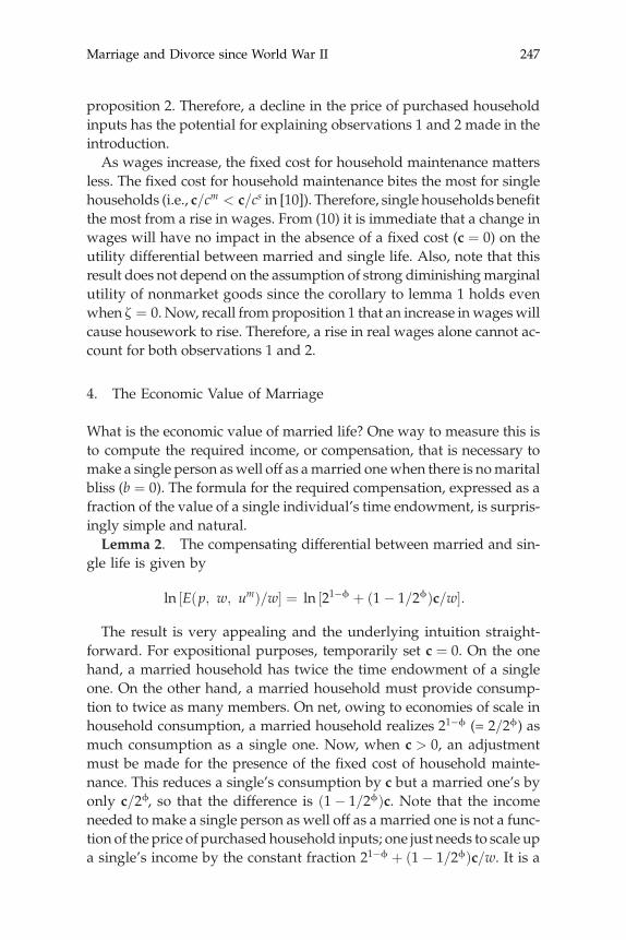
What is the economic value of married life? One way to measure this isto compute the required income, or compensation, that is necessary tomake a single person aswell off as amarried onewhen there is nomaritalbliss (b ¼ 0). The formula for the required compensation, expressed as afraction of the value of a single individual’s time endowment, is surpris-ingly simple and natural.Lemma 2. The compensating differential between married and sin-
gle life is given by
ln ½Eðp; w; umÞ=w� ¼ ln ½21�ϕ þ ð1� 1=2ϕÞc=w�:
The result is very appealing and the underlying intuition straight-forward. For expositional purposes, temporarily set c ¼ 0. On the onehand, a married household has twice the time endowment of a singleone. On the other hand, a married household must provide consump-tion to twice as many members. On net, owing to economies of scale inhousehold consumption, a married household realizes 21�ϕ (= 2=2ϕ) asmuch consumption as a single one. Now, when c > 0, an adjustmentmust be made for the presence of the fixed cost of household mainte-nance. This reduces a single’s consumption by c but a married one’s byonly c=2ϕ, so that the difference is ð1� 1=2ϕÞc. Note that the incomeneeded to make a single person as well off as a married one is not a func-tion of the price of purchased household inputs; one just needs to scale upa single’s income by the constant fraction 21�ϕ þ ð1� 1=2ϕÞc=w. It is a
Greenwood and Guner248
function of the wage rate, though. At higher wage rates the fixed costbites less. Finally, lemma 2 establishes that there is an economic in-centive for marriage provided that there is some form of economiesof scale in consumption or production, that is, whenever either c > 0or ϕ < 1.It may seem a bit puzzling that a fall in price reduces the utility dif-
ferential between married and single life, um � us, but has no impact onthe compensating differential between these two situations, ln ½21�ϕ þð1� 1=2ϕÞc=w�. This is true even when c ¼ 0; that is, the impact of priceon the difference in utility between married and single life is not due tothe presence of the fixed cost. Suppose that one makes the compensa-tion outlined by lemma 2. Then, married and single households will uselaborsaving products in the same intensity, in the sense that dm=ðcm�cÞ ¼ ds=ðcs � cÞ.5 After the required compensation is made, a change inprice will have no impact on the utility differential, um � us, as can read-ily be seen from (9). This suggests that the compensating differential isnot a perfect measure to use for tracking over time the impact of tech-nological progress on the utility differential from marriage.
VI. Quantitative Analysis
The household’s dynamic programming problems—a restatement. Given thestatic nature of the household’s time allocation problem (P3), note thatthe dynamic programming problems for single and married house-holds, (P1) and (P2), can be rewritten as
W ¼ Ið1; p; wÞ þ βZ
max ½V′ðb′Þ; W′�dSðb′Þ
and
VðbÞ ¼ Ið2; p; wÞ þ bþ βZ
max ½V′ðb′Þ; W′�dMðb′jbÞ:
Here Iðz; p; wÞ gives the maximal level of momentary utility that az‐person household can obtain, given that the price of purchased house-hold inputs is p and that the wage rate is w. The fact that for a householdof a particular size, z, it is possible to calculate its current level of utility,Iðz; p; wÞ, without regard to its marriage/divorce decision is very use-ful. Given a sequence of prices and wages, fpt; wtg∞t , it possible to com-pute from (P3) the associated sequence of momentary utilities for singleand married households, fIð1; pt; wtÞ; Ið2; pt; wtÞg∞t .
Marriage and Divorce since World War II 249
A. Matching the Model with the Data
In order to simulate the model, numbers must be selected for the var-ious parameters. Except for five of the parameters, almost nothing isknown about appropriate values. Additionally, time series for pricesand wages need to be inputted into the simulation. Values for the mod-el’s parameters either will be assigned on the basis of a priori informa-tion or will be estimated.
1. A Priori Information
Take the model period to be 1 year. In line with convention, set the sub-jective discount factor at 0.96. The discount factor used in decision mak-ingmust reflect the individual’s probability of survival, 1� δ. A person’slife expectancy is 1=δ. Thus, if (marriageable) life expectancy for anadult is taken to be 47 years, then 1=δ ¼ 47. Therefore, set β ¼ 0:96�ð1� 1=47Þ. Next, let ϕ ¼ 0:77. This is in line with the Organization forEconomic Cooperation and Development's household equivalence scalethat treats the second adult in a family as consuming an additional0.7 times the amount of the first adult. Hence, the parameter ϕ solves1=2ϕ ¼ 1=ð1:0þ 0:7Þ. A series for wages can be constructed from theU.S. data. To do this, divide disposable income by hours worked to ob-tain a measure of compensation per hour. The use of disposable incomeshould (partially) take into account the changes in taxes (and transferpayments) that occurred over this time period. Between 1950 and 2000compensation per hour worked rose 3.0 times. Thus, the analysis simplypresumes that wages rise at 100� ln ð3:0Þ=50 ¼ 2:2% per year. Finally,the household production function is characterized by two parameters,namely, κ and θ. These have been estimated byMcGrattan, Rogerson, andWright (1997). Their numbers are used here.6
2. Estimation
The rest of the parameters will be calibrated/estimated. First, a set ofdata targets is picked. These targets summarize the data along five di-mensions: the time allocations for both married and single households,the fraction of the populationmarried, the divorce rate, and themarriagerate. Second, the parameter values in question are then chosen to maxi-mize themodel’s fit with respect to these data targets. Specifically, for thissection, define d~jt to be the jth data target for period t. Let λ be the vectorof parameters to be estimated. The model will yield a prediction for the

Greenwood and Guner250
jth data target as a function of these parameters and time, denoted bydjt ¼ Djðλ; tÞ. The estimation procedure solves
minλ
X5j¼1
�Xt∈T
Ijtωjt ½d
~jt �Djðλ; tÞ�2=
�Xt∈T
I jt
��; ðP5Þ
whereλ≡ ðc; p1950; γ; α; ζ; μs; σs; μm; σm; ρÞ, Ijt ∈ f0; 1g is an indicatorfunction returningavalueof one if there is anobservationatdate t,ω j
t givestheweightassigned to the target, andT ≡ f1950; 1960; . . . ; 2000g.Unlikethe theory, the estimation does not restrict c≥ 0 or ζ < 0; the data will de-cide themagnitudes and signs of these parameters.It is interesting to compare this strategy for picking parameter values
with the conventional one employed in business cycle analysis, discussedin Cooley and Prescott (1995). Business cycle analysis models short‐runfluctuations around a stationary mean. Hence, parameter values aretypically picked so that the model matches up with some relevantlong‐run averages from the data. In contrast, the current analysis fo-cuses on long‐run changes in a nonstationary world. The strong trendsobserved in the data speak to the degree of curvature in tastes and tech-nologies. Thus, the information contained in these trends shouldbe used to estimate parameter values. This is allowed by letting datatargets at different points in time enter into (P5). A discussion of the10 parameters to be estimated and the 16 data targets used to identifythem will now follow.Household technology parameters—time allocations. Obtaining a price
series for purchased household inputs is somewhat problematic. So, atime path of the form pt ¼ p1950 � e�γðt�1950Þ will be estimated here,where γ is the rate of decline in the time price for purchased householdinputs and p1950 is the initial price. The fixed cost for household main-tenance, c, plays an important role in controlling the initial level of mar-ket work expended by singles relative to married households. Nothingis known about its value, so it will also have to be estimated. Thus, threehousehold technology parameters will be estimated: c, p1950, and γ.To match the model up with the data on time allocations, note that
the fraction of time spent by a married household on market work, lm, isgiven by lm ¼ ð2� hmÞ=2. Likewise, the fraction of time spent by a sin-gle household working in the market is ls ¼ 1� hs. Now, note that lm
and l s can be written as functions of the parameters to be estimated,namely, c, p1950, and γ. They are also functions of time, t, and the tasteparameters α and ζ. Thus, write lmt ¼ Lm c; p1950; γ; α; ζ; tð Þ andlst ¼ Ls c; p1950; γ; α; ζ; tð Þ.

Marriage and Divorce since World War II 251
Now, to operationalize the above in (P5), let d~1t ≡ l~mt , D
1ðλ; tÞ ≡Lmðc; p1950; γ; α; ζ; tÞ, d~2t ≡ l~
st , and D2ðλ; tÞ≡ Lsðc; p1950; γ; α; ζ; tÞ
for t ¼ 1950; 1960; . . . ; 1990. Also, set ω1t =2 and ω2
t =2 to be the frac-tions of married and single females in the time t population of women.(Note that ω1
t þ ω2t ¼ 2, the number of data targets for the time alloca-
tions.) The theory developed suggests that the parameters c, p1950, and γwill be important for determining the time paths for hours worked. Asa practical matter, it turns out that the time paths for hours worked largelyidentify the magnitudes of c, p1950, and γ. Note that, as was mentionedearlier, the matching parameters, μs, σs, μm, σm, and ρ, do not even enterinto the Lmð�Þ and Lsð�Þ functions.Taste and matching parameters—vital statistics. There are seven taste
and matching parameters that need to be estimated, namely, α, ζ, μs,σs, μm, σm, and ρ. The parameter α determines the weight of marketgoods in the utility function, and the parameter ζ controls the degreeof concavity in the utility function for nonmarket goods. The more con-cave this utility function is, the faster households will move away fromnonmarket goods toward market goods as income rises. Hence, thisparameter plays an important role in determining how the relative ben-efits of married versus single life respond to technological progress. Theidea here is that information on the trend in vital statistics is importantfor determining the value of ζ. The remaining six matching parametersgovern the noneconomic aspects of marriage. Again recall that Lmð�Þ andLsð�Þ are not functions of the matching parameters.These seven parameters impinge heavily on the model’s predictions
concerning vital statistics. Here, the data are targeted along three dimen-sions for two years, 1950 and 2000: the fraction of the population mar-ried, the divorce rate, and the marriage rate. So, let m~ j
1950and m~ j
2000denote the data targets along the jth dimension for the years 1950 and2000. Correspondingly, permit mj
1950 ¼ Mjðc; p1950; γ; α; ζ; μs; σs;
μm; σm; ρ; 1950Þ and mj2000 ¼ Mjðc; p1950; α; ζ; μs; σs; μm; σm; ρ; 2000Þ
to represent the model’s steady‐state output along the jth dimensionfor the years 1950 and 2000. Hence, in (P5) set d~jþ2
t ≡m~ jt , D
jþ2ðλ; tÞ ≡Mjðc; p1950; γ; α; ζ; μs; σs; μm; σm; ρ; tÞ, and ω jþ2
t¼ 1, for j = 1, 2, 3
and t = 1950 and 2000. (Again, note that ω3t þ ω4
t þ ω5t ¼ 3, the number
of data targets for the vital statistics.)In summary, the parameter vector λ≡ ðc; p1950; γ; α; ζ; μs; σs; μm;
σm; ρÞ is estimated so that the model matches the data on five dimen-sions: the time allocations for married households, the time allocationsfor single households, the fraction of the population married, the di-vorce rate, and the marriage rate. This involves 16 observations from
Greenwood and Guner252
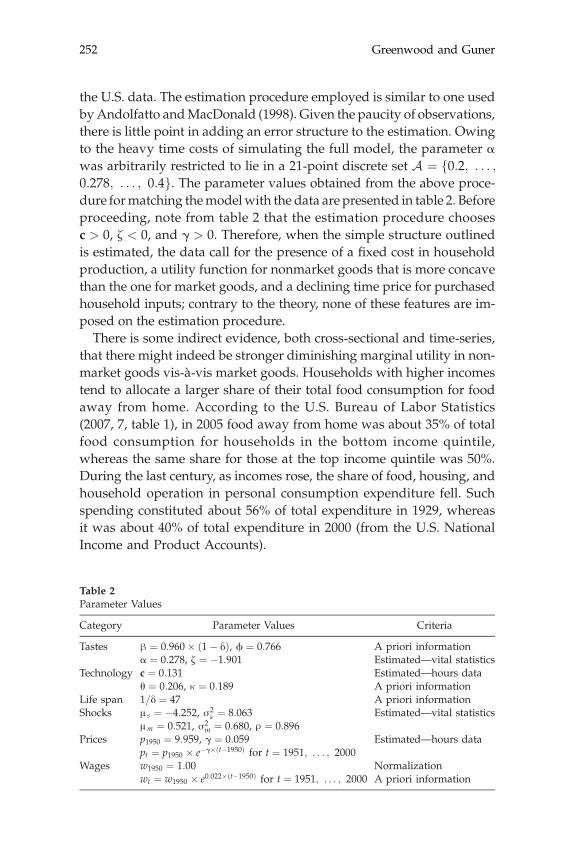
the U.S. data. The estimation procedure employed is similar to one usedbyAndolfatto andMacDonald (1998). Given the paucity of observations,there is little point in adding an error structure to the estimation. Owingto the heavy time costs of simulating the full model, the parameter αwas arbitrarily restricted to lie in a 21‐point discrete set A ¼ f0:2; . . . ;
0:278; . . . ; 0:4g. The parameter values obtained from the above proce-dure formatching themodelwith the data are presented in table 2. Beforeproceeding, note from table 2 that the estimation procedure choosesc > 0, ζ < 0, and γ > 0. Therefore, when the simple structure outlinedis estimated, the data call for the presence of a fixed cost in householdproduction, a utility function for nonmarket goods that is more concavethan the one for market goods, and a declining time price for purchasedhousehold inputs; contrary to the theory, none of these features are im-posed on the estimation procedure.There is some indirect evidence, both cross‐sectional and time‐series,
that there might indeed be stronger diminishing marginal utility in non-market goods vis‐à‐vis market goods. Households with higher incomestend to allocate a larger share of their total food consumption for foodaway from home. According to the U.S. Bureau of Labor Statistics(2007, 7, table 1), in 2005 food away from home was about 35% of totalfood consumption for households in the bottom income quintile,whereas the same share for those at the top income quintile was 50%.During the last century, as incomes rose, the share of food, housing, andhousehold operation in personal consumption expenditure fell. Suchspending constituted about 56% of total expenditure in 1929, whereasit was about 40% of total expenditure in 2000 (from the U.S. NationalIncome and Product Accounts).
Table 2Parameter Values
Category
Parameter Values CriteriaTastes
β ¼ 0:960� ð1� δÞ, ϕ ¼ 0:766 A priori information α ¼ 0:278, ζ ¼ �1:901 Estimated—vital statisticsTechnology
c ¼ 0:131 Estimated—hours data θ ¼ 0:206, κ ¼ 0:189 A priori informationLife span
1=δ ¼ 47 A priori information Shocks μ s ¼ �4:252, σ2s ¼ 8:063
Estimated—vital statistics μm ¼ 0:521, σ2m ¼ 0:680, ρ ¼ 0:896
Prices p1950 ¼ 9:959, γ ¼ 0:059 Estimated—hours datapt ¼ p1950 � e�γ�ðt�1950Þ for t ¼ 1951; . . . ; 2000
Wages w1950 ¼ 1:00 Normalizationwt ¼ w1950 � e0:022�ðt�1950Þ for t ¼ 1951; . . . ; 2000
A priori information
Marriage and Divorce since World War II 253
B. Results
Visualize the economy in 1950. Wages are low and the price for pur-chased household inputs is high, at least relative to 2000. Over time,wages grow and the price for purchased household inputs falls. Thetime paths for wages and prices inputted into the analysis are shownin figure 4. As can be seen, in the U.S. data, wages increase 3.0 timesover the time period in question. Prices are estimated to decline by afactor of 20. This seems large, but it is merely the result of compoundinga 6.0% annual decline over a 50‐year period. Can these two facts helpto explain the decline in marriage and the rise in divorce over the last50 years? This is the question asked here.
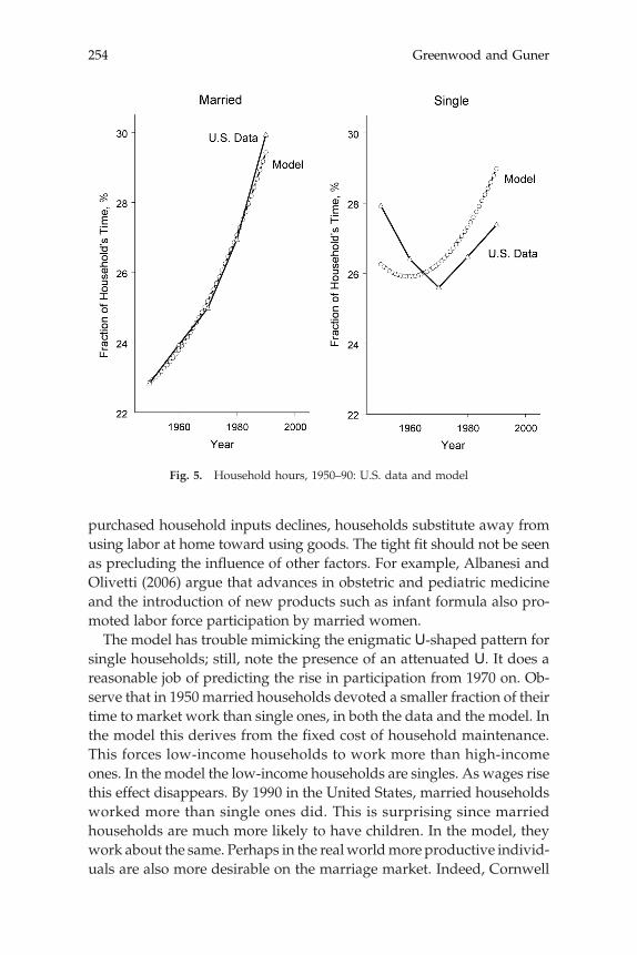
1. Household Hours
The time path for household hours that arises from the model is shownin figure 5. It mimics the U.S. data reasonably well. In particular, themodel matches very well the sharp increase in the fraction of time de-voted tomarketwork bymarried households. This is due to the decliningprice for purchased household inputs. Purchased household inputsand housework are substitutes in household production. As the price of
Fig. 4. Wages and prices, 1950–2000: model inputs
Greenwood and Guner254
purchased household inputs declines, households substitute away fromusing labor at home toward using goods. The tight fit should not be seenas precluding the influence of other factors. For example, Albanesi andOlivetti (2006) argue that advances in obstetric and pediatric medicineand the introduction of new products such as infant formula also pro-moted labor force participation by married women.The model has trouble mimicking the enigmatic U‐shaped pattern for
single households; still, note the presence of an attenuated U. It does areasonable job of predicting the rise in participation from 1970 on. Ob-serve that in 1950 married households devoted a smaller fraction of theirtime to market work than single ones, in both the data and the model. Inthe model this derives from the fixed cost of household maintenance.This forces low‐income households to work more than high‐incomeones. In the model the low‐income households are singles. As wages risethis effect disappears. By 1990 in the United States, married householdsworked more than single ones did. This is surprising since marriedhouseholds are much more likely to have children. In the model, theywork about the same. Perhaps in the realworldmore productive individ-uals are also more desirable on the marriage market. Indeed, Cornwell
Fig. 5. Household hours, 1950–90: U.S. data and model

Marriage and Divorce since World War II 255
and Rupert (1997) provide evidence that this is the case. Such a marriageselection effect is missing in the model.The estimation procedure picks a 6.0% annual rate of price decline, as
was mentioned. This looks reasonable. For instance, the Gordon quality‐adjusted time price index for air conditioners, clothes dryers, dish-washers, microwaves, refrigerators, televisions, videocassette recorders,and washing machines fell at 10% a year over the postwar period. Al-ternatively, one could take the price of kitchen and other householdappliances from the National Income and Product Accounts. Thisprice series declined, relative towage growth, at about 1.5% a year since1950. The 6% estimate obtained here is the midpoint of these twonumbers.
2. Vital Statistics
Now, the model starts off from an initial steady state that resembles theUnited States in 1950 and converges to a final one looking like theUnited States in 2000. In 1950 about 81.6% of the female populationwas married (out of nonwidows who were between the ages of 18 and64). There were 10.6 divorces per 1,000 married females and 211 mar-riages. According to Schoen (1983), marriages lasted about 30 years in1950. In 2000 the picture was quite different. Only 62.5% of females weremarried. The divorce rate had risen to 23 divorces by 1995, and the mar-riage rate had declined to about 80 marriages. Finally, the average dura-tion of marriages was about 20–24 years.7 Table 3 shows the model’sperformance along these dimensions. Note that singles face a distribu-tion with a low mean and a high variance, whereas married people facea distribution that has a relatively high mean, a low variance, and a highautocorrelation (see table 2). This has two effects. First, it encouragessingles to wait a while until a good match comes along. Second, it gen-erates the long durations of marriages observed in the data.
Table 3Initial and Final Steady States
1950
2000Model
Data Model DataFraction married
.816 .816 .694 .625 Probability of divorce .011 .011 .024 .023 Probability of marriage .129 .211 .096 .082 Duration of marriages 31.36 29.63 22.47 20–24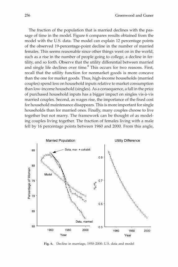
Greenwood and Guner256
The fraction of the population that is married declines with the pas-sage of time in the model. Figure 6 compares results obtained from themodel with the U.S. data. The model can explain 12 percentage pointsof the observed 19‐percentage‐point decline in the number of marriedfemales. This seems reasonable since other things went on in the world,such as a rise in the number of people going to college, a decline in fer-tility, and so forth. Observe that the utility differential between marriedand single life declines over time.8 This occurs for two reasons. First,recall that the utility function for nonmarket goods is more concavethan the one for market goods. Thus, high‐income households (marriedcouples) spend less on household inputs relative to market consumptionthan low‐income household (singles). As a consequence, a fall in the priceof purchased household inputs has a bigger impact on singles vis‐à‐vismarried couples. Second, as wages rise, the importance of the fixed costfor householdmaintenance disappears. This is more important for singlehouseholds than for married ones. Finally, many couples choose to livetogether but not marry. The framework can be thought of as model-ing couples living together. The fraction of females living with a malefell by 16 percentage points between 1960 and 2000. From this angle,
Fig. 6. Decline in marriage, 1950–2000: U.S. data and model
Marriage and Divorce since World War II 257
the model captures about 75% of the decline between 1950 and 2000.Interestingly, the model seems to dowell predicting the number of mar-riages for the first half of the sample and the number of cohabitationsfor the later half.Underlying the decline in the fraction of the U.S. population that is
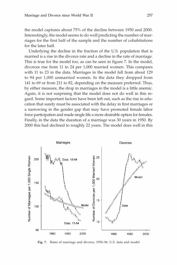
married is a rise in the divorce rate and a decline in the rate of marriage.This is true for the model too, as can be seen in figure 7. In the model,divorces rise from 11 to 24 per 1,000 married women. This compareswith 11 to 23 in the data. Marriages in the model fall from about 129to 94 per 1,000 unmarried women. In the data they dropped from141 to 69 or from 211 to 82, depending on the measure preferred. Thus,by either measure, the drop in marriages in the model is a little anemic.Again, it is not surprising that the model does not do well in this re-gard. Some important factors have been left out, such as the rise in edu-cation that surely must be associated with the delay in first marriages ora narrowing in the gender gap that may have promoted female laborforce participation andmade single life amore desirable option for females.Finally, in the data the duration of a marriage was 30 years in 1950. By2000 this had declined to roughly 22 years. The model does well in this
Fig. 7. Rates of marriage and divorce, 1950–96: U.S. data and model

Greenwood and Guner258
regard. It predicts that the duration of a marriage was 31 years in 1950and 22 years in 2000.
VII. 1920–2000: A Proposed Extension
The effects of technological progress on the formation of householdswere beginning to percolate before World War II. How are these effectsmanifested in the data? Can the model be modified to address them?
A. The Marriage Data
Figure 8 plots the proportion of the female population that was marriedfrom 1880 to 2000. About 72% of the population was married in 1900, asopposed to 62% in 2000. So, 10 percentage points fewer women weremarried at the end of the twentieth century relative to the beginning.Observe that the number of marriages shows a hump‐shaped patternroughly coinciding with the baby boom years. This pattern is not asdramatic as it seems at first glance, though. The population was muchyounger at the turn of the last century than it is today. Women aged 18–24made up 28%of the population in 1900. Now they account for 15%. Youngwomen are much less likely to be married than older ones. Figure 8also shows the fraction of the female population that are married after
Fig. 8. Marriage, 1880–2000
Marriage and Divorce since World War II 259
a correction is made for the shift in the age distribution. First, note thatmany more females were married at the beginning of the century than atthe end, about 17 percentage points more. Second, the hump is still there,but it is much less pronounced. What can account for this hump‐shapedpattern in marriage? Specifically, why did the number of marriages risebetween 1940 and 1960 and subsequently decline?
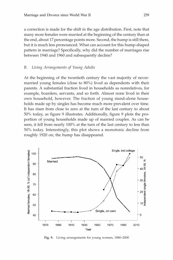
B. Living Arrangements of Young Adults
At the beginning of the twentieth century the vast majority of never‐married young females (close to 80%) lived as dependents with theirparents. A substantial fraction lived in households as nonrelatives, forexample, boarders, servants, and so forth. Almost none lived in theirown household, however. The fraction of young stand‐alone house-holds made up by singles has become much more prevalent over time.It has risen from close to zero at the turn of the last century to about50% today, as figure 9 illustrates. Additionally, figure 9 plots the pro-portion of young households made up of married couples. As can beseen, it fell from nearly 100% at the turn of the last century to less than50% today. Interestingly, this plot shows a monotonic decline fromroughly 1920 on; the hump has disappeared.
Fig. 9. Living arrangements for young women, 1880–2000

Greenwood and Guner260
C. Returning to the Hypothesis
The idea here is that technological progress in the household sectormade it feasible to establish smaller and smaller households. In the ini-tial stages of development, technological advance made it easier for ayoung adult to leave his or her parents’ home and marry. As householdtechnology progressed further, it became viable for young adults to leavehome and remain single. Therefore, themove by young adults from largeto two‐person households coincided with an increase in marriageswhereas the subsequent shift toward one‐person households was asso-ciated with a decline. This hypothesis is consistent with the decline in thefraction of total young households made up of married ones that wasshown in figure 9.
1. Altering the Setup
To gauge whether or not this hypothesis has promise, consider the fol-lowing simple extension of the model. Let there now be three types ofindividuals: singles living at home with their families (dubbed youngadults), singles living in their own homes, and married couples livingin their own households. Suppose that a young adult living with hisfamily receives a momentary utility ofH � x. HereH gives the economicbenefit from living at home, as a function of the underlying state of theeconomy (w, p). The variable x represents the psychic disutility from liv-ing at home (vs. alone), so to speak. Each single starts adulthood living athomewith his or her parents and sibling. Assume that a young adult firstleaves home single and then looks for amate. In particular, he or she exitsthe family nest with probability ε. This probability is a choice variable,which is dependent on the amount of effort that the youngster in-vests in leaving home. Let the convex cost function for leaving home,C : ½0; 1�→ Rþ, be specified by
CðεÞ ¼ ιε1þχ
1þ χfor χ > 0:
Once departed, the youngster can never return. Also, presume that afamily realizes no benefit (or incurs a cost) from a child staying at home.The rest of the setup remains the same as before. The analysis will focuson steady states.
Marriage and Divorce since World War II 261
Let Y be the expected lifetime utility for a young adult who is cur-rently living at home. His dynamic programming problem is givenby
Y ¼ H � xþ β max0≤ε≤1
�εZ
max ½VðbÞ; W �dSðbÞ þ ð1� εÞY� CðεÞ�:
The solution for ε is given by
ε ¼�R
max ½VðbÞ; W�dSðbÞ � Yι
�1=χfor 0≤
Zmax ½VðbÞ; W�dSðbÞ � Y≤ι:
As can be seen, a youngster will be more diligent about leaving homewhen the gains from entering the singles market,
Rmax ½VðbÞ; W�dSðbÞ,
are high relative to the benefits of staying at home, Y. Now, consideran increase in wages or a fall in prices. These will lead to reductions inthe number of young adults living at home, as long as the benefits of in-dependent single life rise more than the benefits of a dependent one, thatis, as long as ∂
Rmax ½VðbÞ; W�dSðbÞ=∂w > ∂Y=∂w or ∂
Rmax ½VðbÞ;
W�dSðbÞ=∂p < ∂Y=∂p. The considerations ensuring this parallel thoseoutlined in Section V.Note that problems (P1) and (P2) remain the same as before, since the
decision to leave home is irreversible and because a married couple real-izes no utility from a child living at home. In a steady state the equationspecifying the type distribution for marriages will appear as
MðbÞ ¼ ð1� δÞZ Z
M∩½�∞;b�dMð b~ jb�1ÞdMðb�1Þ
þ ½ð1� δÞsþ ð1� δÞεyþ δε�ZM∩½�∞;b�
dSðb~Þ;
where the number of young adults living at homewith their parents, y, isgiven by
y ¼ δð1� εÞ1� ð1� δÞð1� εÞ ;
and ZdMðbÞ þ sþ y ¼ 1
(cf. [5]). Therefore, a huge virtue of this setup is that it involves littlemod-ification to the original formulation.
Greenwood and Guner262
2. An Example
Does the above setup have promise for extending the earlier analysis tothe pre–World War II period? To address this question, the model’s po-tential will be demonstrated using a simple example. The example willfocus on three years, to wit, 1920, 1950, and 2000. For each year the model’ssteady state will be computed. The output from the model will thenbe compared with the stylized facts discussed in Sections VII.A andB. It should be emphasized that given the simplicity of the setup, theexample is intended only as an illustration; it should not be viewedas a serious data‐fitting exercise.For the taste and technological parameters, take the values presented
in table 2 with two changes. Presumably the price for purchased house-hold inputs fell faster earlier in the last century than later on. So allowthe price to fall at the constant rate γ1920 prior to 1950. Additionally, thefixed cost for household formation will be allowed to differ for this sub-period as well. Denote this by c1920. The above setup changes the poolof singles that are available on the marriage market. So, new matchingparameters will be selected. These values will apply for the whole1920–2000 period. Something must be specified for the economic benefitthat a young adult derives from staying at homewithhis parents,Hðw; pÞ.Simply suppose that each family has two kids and set Hðw; pÞ ¼Ið4; p; wÞ. That is, each period a young adult who stays at home realizesthe maximal level of momentary utility that would arise in a householdwith four wage earners. (One could just as easily setHðw; pÞ ¼ ϑIð4; p;wÞ for some ϑ∈ ð0; 1Þ. The essential requirement is that the economicbenefit of living in a large household should decline over time relativeto a small one.) Given the primitive nature of the example, the param-eter values are selected so that the model’s steady states display somefeatures of interest, discussed below. The parameter values selected arepresented in table 4.In the model, 63.8% of single women work in 1920, the same number
as in the data for women between the ages of 18 and 64 (see table 5).
Table 4New Parameter Values: Example
Household production
c1920 ¼ 0:161, γ1920 ¼ 0:165 Shocks μ s ¼ �3:75, σ2s ¼ 8
μm ¼ 0:145, σ2m ¼ 0:28, ρ ¼ 0:59
Utility of living at home Hðw; pÞ ¼ Ið4; p; wÞx ¼ 2:051
Utility cost of leaving home ι ¼ 115:27, χ ¼ 1:083
Marriage and Divorce since World War II 263
Likewise, only 7.8% of married women work in 1920, again the same asis observed in the data. By construction, the model still generates thehours‐worked predictions shown in figure 5 for the period 1950–90.This transpires because the hours‐worked decisions are functions solelyof the taste and technology parameters, and these have not been changedfor the 1950–2000 period. Table 6 presents the results for some vital sta-tistics. The statistics for the U.S. data apply to women in the 18–64 agegroup (as in table 3). The numbers have also been adjusted for the shiftin U.S. age distribution, whichwas discussed earlier. First, as can be seen,the model replicates quite nicely the stylized facts for the fraction of fe-males who are married. In particular, the model duplicates the hump‐shaped pattern displayed in the data. An improvement in fitting thenumbers for 2000 can be obtained at the sacrifice of a diminution in theleft‐hand side of the hump. Second, it also does a reasonable job of pre-dicting the decline in the proportion of single females who live at homewith their parents. Third, analogously, it mimics well the rise in the frac-tion of single females who live alone. Fourth, the number of adults livingin a household declinedmonotonically over the course of the last century,as table 6 shows. This is true for the model as well. The model cannotmatch the steepness of this decline. One reason might be that fertility de-clined in theUnited States over this time period, and the population agedsignificantly. The elderly are much more likely to live alone now, relativeto the past. Themodel, of course, assumes that eachwoman always givesbirth to two children. All in all, it looks as though an extension of theframework that models the decision of a young adult to leave home
Table 6Household Living Arrangements
1920
1950 2000Model
Data Model Data Model DataMarried: m
.796 .791 .819 .819 .680 .616 Single, living at home: y .185 .185 .125 .125 .109 .109 Single, living alone: s .019 .024 .056 .056 .212 .275 Household size: number of adults 2.40 2.55 2.15 2.14 1.81 1.65Table 5Participation Rates, 1920
Model
DataMarried
.078 .078 Single .638 .638
Greenwood and Guner264
has promise for explaining the trends in vital statistics that are observedin the U.S. data.
3. Discussion
The proposed extension of the benchmark model is minimalist, to saythe least. It is easy to identify areas of the analysis that warrant furtherwork. At the heart of the above extension is a young adult’s decision toleave home. Perhaps one could allow for a young adult to search for amate while at home. Three options would then arise: stay at home, leavehome married, and leave home single. Doing this will be important formatching the rates ofmarriage that are observed in the data. In the earlierpart of the last century most females got engaged before they left home.Therefore, the model cannot hope to match the observed rates of mar-riage at early dates if marriageability is restricted to the small pool ofsingle females living alone. Additionally, should searching for a matewhile living in your parents’ home be as efficient as searching for onewhen you live alone?Modeling the utility that a young adult receiveswhileat home is another area in which the framework could be improved. Dotransfers flow from young adults to parents or vice versa? The answer tothis will depend on how parents care about their kids, how children feelabout their parents, and their mode of interaction.The economic forces that reduce the relative benefit of single versus
married life may also have affected other living arrangements, suchas the incentives of the elderly to live with their kids. Between 1970and 1990 the fraction of widows living alone rose from 52.1% to 64.2%.Bethencourt and Rios‐Rull (2009) argue that the rise in the relative in-come of elderly widows can account for a significant part of the rise inthe number of elderly widows living alone between 1970 and 1990. Ina similar vein, Schoellman and Tertilt (2007) argue that a substantial pro-portion of the decline in household size is due to an increased demand forprivacy, made possible by rising living standards.
VIII. Some Cross‐Country Evidence on Household Size
The above theory suggests that as the relative price of purchased house-hold inputs declines, so should the number of adults living in a house-hold. The relationship between household size and price is displayed inthe upper panel of figure 10 for a small sample of Western countries forthe year 2001. As can be seen, there is a positive association between thesetwo variables. Of course, other things may affect household size in a

Marriage and Divorce since World War II 265
country. To take into account such factors, a linear regression of the fol-lowing form is estimated:
SIZE¼CONSTANTþβ�PRICEþγ�CONTROLSþε;
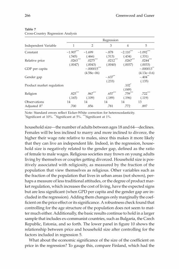
with ε∼Nð0; σÞ, where CONTROLS represents a vector of control vari-ables. A list of potential control variables might include GDP per cap-ita, the gender gap, the extent of urbanization, the amount of productmarket regulation, and the religiosity of a population. The empirical anal-ysis is in the spirit of Cavalcanti and Tavares (2008) and Algan and Cahuc(2007), who examined, using a panel of countries, the impact of applianceprices on female labor supply and younger and older (non‐prime‐age)workers, respectively. Theory suggests that β should be positive. Thesize of this coefficient is also of interest because it indicates the powerof the relative price effect.The results of the analysis are presented in table 7. They should be
interpreted with the utmost caution because the sample size is so small.Focus attention on regression 5. All the variables are statistically signifi-cant and enter in with the expected sign. The price effect in the regressionis highly significant. One would expect, as per capita GDP rises, that
Fig. 10. Cross‐country relationship between household size and the relative price ofappliances, 2001.
Greenwood and Guner266
household size—the number of adults between ages 18 and 64—declines.Females will be less inclined to marry and more inclined to divorce, thehigher their wage rate relative to males, since this makes it more likelythat they can live an independent life. Indeed, in the regression, house-hold size is negatively related to the gender gap, defined as the ratioof female to male wages. Religious societies may frown on young adultsliving by themselves or couples getting divorced. Household size is pos-itively associated with religiosity, as measured by the fraction of thepopulation that view themselves as religious. Other variables such asthe fraction of the population that lives in urban areas (not shown), per-haps ameasure of less traditional attitudes, or the degree of productmar-ket regulation, which increases the cost of living, have the expected signsbut are less significant (when GPD per capita and the gender gap are in-cluded in the regression). Adding them changes onlymarginally the coef-ficient on the price effect or its significance. A robustness check found thatcontrolling for the age structure of the population does not seem to mat-termuch either. Additionally, the basic results continue to hold in a largersample that includes ex‐communist countries, such as Bulgaria, the CzechRepublic, Estonia, and so forth. The lower panel in figure 10 shows therelationship between price and household size after controlling for thefactors included in regression 5.What about the economic significance of the size of the coefficient on
price in the regression? To gauge this, compare Finland, which had the
Table 7Cross‐Country Regression Analysis
Regression
Independent Variable
1 2 3 4 5Constant
−1.907*** −1.699 −.878 −2.110*** −1.092***(.545)
(.466) (.513) (.434) (.331) Relative price .0263*** .0275*** .0212*** .0267*** .0244***(.0047)
(.0043) (.0040) (.0037) (.0033) GDP per capita −.000015*** −.000013**(4.58e−06)
(4.13e−0.6) Gender gap −.637** −.404**(.233)
(.135) Product market regulation .102*(.049)
Religion .825*** .867*** .657*** .759*** .722***(.165)
(.109) (.189) (.196) (.119) Observations 14 14 14 14 13 Adjusted R2 .700 .856 .781 .772 .897Note: Standard errors reflect Eicker‐White correction for heteroscedasticity.*Significant at 10%. **Significant at 5%. ***Significant at 1%.
Marriage and Divorce since World War II 267
lowest relative price level of 104.8, with Ireland, which had the highestrelative price level of 122.01. The relative price difference is associatedwith about 0.44 member per household (about 100% of the observeddifference, from 1.424 for Finland to 1.879 for Ireland). This price effectis quantitatively powerful. An increase in per capita GDP from $17,440(Greece with a household size of 1.86) to $34,320 (the United States witha household size of 1.65) leads to a drop in household size of 0.22 mem-ber (again almost all of the difference between the two countries). Bycomparison, the gender gap has a much weaker impact. Suppose thatthe gender gap shrinks from 0.4 (Ireland, the widest) to 0.7 (Denmark,the narrowest). Household size falls by 0.12 member, which represents25% of the difference. Thus, the forces stressed in the paper appear tohave a strong impact on household size.
IX. Conclusions
The fraction of adult females who are married has dropped by roughly20 percentage points since World War II. Females now spend a muchsmaller part of their adult life married than 50 years ago. Associatedwith this has been a rise in the divorce rate and a decline in the rate ofmarriage. At the same time, hours worked by married households roseconsiderably. This was driven by a large increase in labor force participa-tion by married females.An explanation of these facts is offered here. The story told focuses
on technological progress in both the household and market sectors.The idea is that investment‐specific technological progress in the house-hold sector reduced the need to use labor at home. This simultaneouslyallowed women to enter the labor force and eroded the economic incen-tives for marriage. The analysis blends together a search model of mar-riage and divorce with a model of household production. The economicincentives formarriage derive from economies of scale in household pro-duction. These are whittled away over time for two reasons. First, risingwagesmake it easier tomeet or exceed the fixed cost for householdmain-tenance. This reduces the need to marry to make ends meet. Second, afalling price for laborsaving household inputs has a bigger impact on sin-gle vis‐à‐vis married households, since the former devote a larger shareof their spending to these products as a result of a high rate of diminish-ing marginal utility for nonmarket consumption. These two effects in-crease the (relative) value of single life.So, where can the analysis go from here? Technological progress in
the home and market may affect the pattern of matching in society.

Greenwood and Guner268
There is some evidence that the degree of assortative mating in the UnitedStates has increased since 1940.9 Extensions of the model may be able tocapture this. Suppose that individuals differ in their labor market pro-ductivities. Assume that married males devote all their time to marketwork whereas married females split their time between market workand household work. Now, when they choose a potential mate, theirearnings in the labor market will be a consideration. This will matter lessat early stages of economic development, since married women will dolittlemarketwork because of the large amount of time spent in householdproduction. As women start to work more in the market, owing to tech-nological progress, it will begin tomattermore. As an economy advancesand the benefits from economies of scale in household consumption dimin-ish, earnings potential along with marital bliss will become more im-portant criteria when choosing amate. The degree of assortativematingwill increase. Additionally, such an analysis would likely imply thatthe drop in the marriage rate should be biggest for those individualsin lower‐income groups, since the relative benefits from marriage willfall themost for them. Indeed, there is some evidence suggesting that thishas been the case.10
Appendix
A. Proofs
As a prelude to the proofs of the lemmas and propositions, combine (7)and (8) to obtain
d ¼� ð1� θÞp
θ
�1=ðκ�1Þh ≡ RðpÞh: ðA1Þ
Using this in (6) then gives
c� c ¼ w��
z� cw
�� h
�� wpd ¼ w
��z� c
w
�� h
�� wpRðpÞh: ðA2Þ
Finally, by substituting (A1) and (A2) into (8), a single equation can beobtained in one unknown, namely h:
α½θRðpÞκ þ ð1�θÞ�1�ζ=κh1�ζ ¼ ð1� αÞð1� θÞz�ϕζ��
z� cw
�� h�pRðpÞh
�:
ðA3Þ
Marriage and Divorce since World War II 269
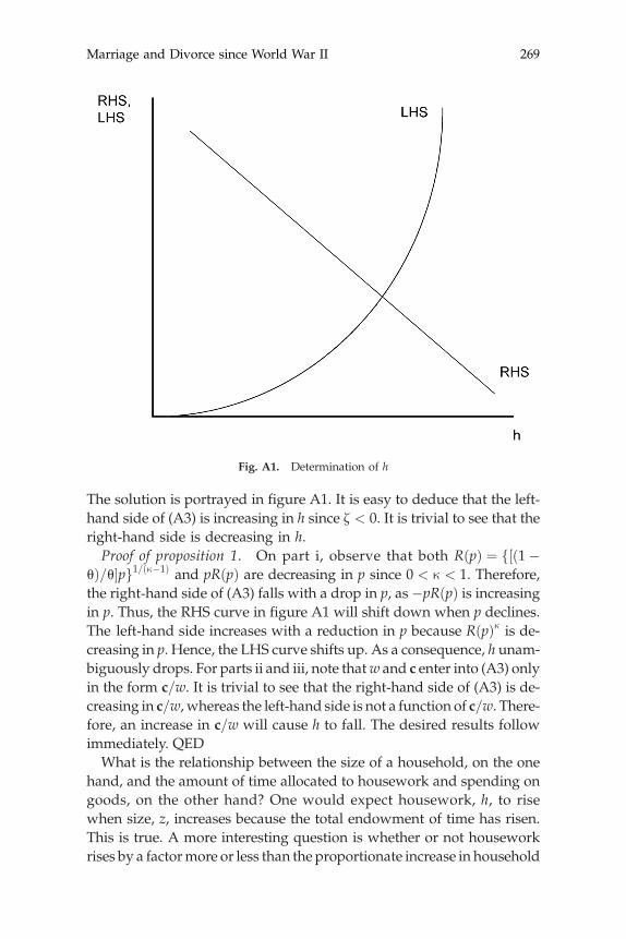
The solution is portrayed in figure A1. It is easy to deduce that the left‐hand side of (A3) is increasing in h since ζ < 0. It is trivial to see that theright‐hand side is decreasing in h.Proof of proposition 1. On part i, observe that both RðpÞ ¼ f½ð1�
θÞ=θ�pg1=ðκ�1Þ and pRðpÞ are decreasing in p since 0 < κ < 1. Therefore,the right‐hand side of (A3) falls with a drop in p, as �pRðpÞ is increasingin p. Thus, the RHS curve in figure A1 will shift down when p declines.The left‐hand side increases with a reduction in p because RðpÞκ is de-creasing in p. Hence, the LHS curve shifts up. As a consequence, h unam-biguously drops. For parts ii and iii, note thatw and c enter into (A3) onlyin the form c=w. It is trivial to see that the right‐hand side of (A3) is de-creasing in c=w, whereas the left‐hand side is not a function of c=w. There-fore, an increase in c=w will cause h to fall. The desired results followimmediately. QEDWhat is the relationship between the size of a household, on the one
hand, and the amount of time allocated to housework and spending ongoods, on the other hand? One would expect housework, h, to risewhen size, z, increases because the total endowment of time has risen.This is true. A more interesting question is whether or not houseworkrises by a factormore or less than the proportionate increase in household
Fig. A1. Determination of h

Greenwood and Guner270
size. On the one hand, given that the utility function for nonmarket goodsis more concave than the one for market goods, the household has a pref-erence for diverting extra resources into market consumption. This sug-gests that housework will increase less than proportionately with size.On the other hand, at higher levels of income the fixed cost for householdmaintenance will matter less. This suggests that housework will risemore than proportionately with size. While the result turns out to be am-biguous, a useful upper bound on the response of housework to house-hold size can be derived. This is presented in lemma 3, which is animportant step toward proving proposition 2. With this upper bound,it can be shown that married households spend less than single house-holds do on the inputs into household production, d and h, at least rela-tive to market consumption, c� c.Lemma 3. A rise in z by a factor of λ > 1 leads to an increase in h by
a factor strictly less than ρ ¼ ðλz� c=wÞ=ðz� c=wÞ.When ζ ¼ 0 (ln utilityfor nonmarket goods), amagnification in z by a factor ofλ > 1will cause hto expand by exactly a factor of ρ.Proof. Rewrite equation (A3) as
α½θRðpÞκ þ ð1� θÞ�1�ζ=κh�ζhþ ð1� αÞð1� θÞ½1þ pRðpÞ�z�ϕζh ¼ð1� αÞð1� θÞz�ϕζðz� c=wÞ:
If z increases by a factor λ > 1, then z� c=w rises by the factor ρ ≡ðλz� c=wÞ=ðz� c=wÞ > λ. Now, the right‐hand side rises by the factorλ�ϕζρ. Observe that if h rises by the factor ρ, then the left‐hand side willincrease by more than the factor λ�ϕζρ, because ρ�ζ > λ�ϕζ when ζ < 0and 0 < ϕ < 1. Therefore, to restore equality between the left‐hand andright‐hand sides of the above equation, h must rise by less than the fac-tor ρ. The first part of the lemma has been established. Finally, supposethat ζ ¼ 0. In this case, (A3) reduces to
h ¼ ð1� αÞð1� θÞðz� c=wÞα½θRðpÞκ þ ð1� θÞ� þ ð1� αÞð1� θÞ½1þ pRðpÞ� : ðA4Þ
The second part of the lemma follows immediately. QEDIn line with the intuition presented above on the relationship be-
tween household size and allocations, suppose that c ¼ 0. In this case,ρ ¼ λ. Thus, larger households will devote proportionately less of theirtime to housework than smaller ones, since an increase in householdsize by a factorλ > 1will lead toa rise in hbya factor less thanρ ¼ λ.Next,suppose that ζ ¼ 0 and c > 0, so that both market goods and nonmarket
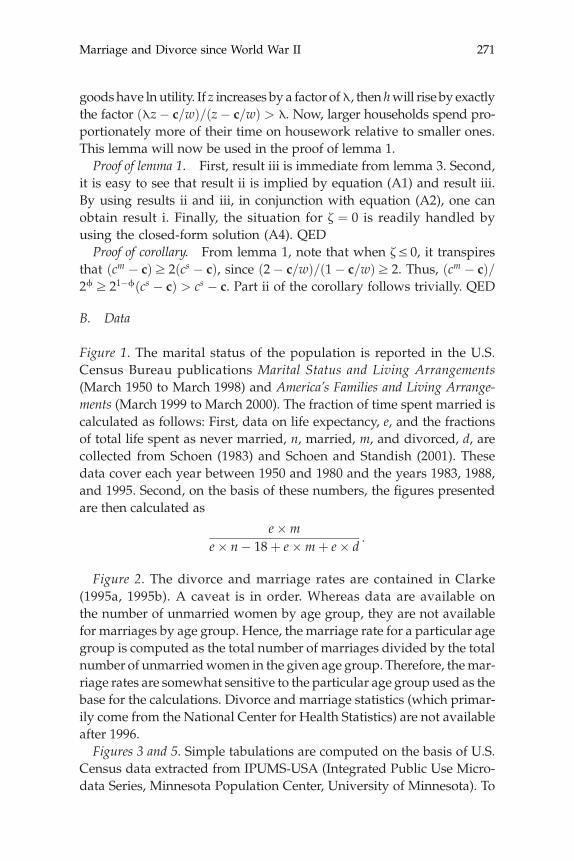
Marriage and Divorce since World War II 271
goodshave ln utility. If z increases by a factor ofλ, then hwill rise by exactlythe factor ðλz� c=wÞ=ðz� c=wÞ > λ. Now, larger households spend pro-portionately more of their time on housework relative to smaller ones.This lemma will now be used in the proof of lemma 1.Proof of lemma 1. First, result iii is immediate from lemma 3. Second,
it is easy to see that result ii is implied by equation (A1) and result iii.By using results ii and iii, in conjunction with equation (A2), one canobtain result i. Finally, the situation for ζ ¼ 0 is readily handled byusing the closed‐form solution (A4). QEDProof of corollary. From lemma 1, note that when ζ≤ 0, it transpires
that ðcm � cÞ≥ 2ðcs � cÞ, since ð2� c=wÞ=ð1� c=wÞ≥ 2. Thus, ðcm � cÞ=2ϕ ≥ 21�ϕðcs � cÞ > cs � c. Part ii of the corollary follows trivially. QED
B. Data
Figure 1. The marital status of the population is reported in the U.S.Census Bureau publications Marital Status and Living Arrangements(March 1950 to March 1998) and America’s Families and Living Arrange-ments (March 1999 to March 2000). The fraction of time spent married iscalculated as follows: First, data on life expectancy, e, and the fractionsof total life spent as never married, n, married, m, and divorced, d, arecollected from Schoen (1983) and Schoen and Standish (2001). Thesedata cover each year between 1950 and 1980 and the years 1983, 1988,and 1995. Second, on the basis of these numbers, the figures presentedare then calculated as
e�me� n� 18þ e�mþ e� d
:
Figure 2. The divorce and marriage rates are contained in Clarke(1995a, 1995b). A caveat is in order. Whereas data are available onthe number of unmarried women by age group, they are not availablefor marriages by age group. Hence, the marriage rate for a particular agegroup is computed as the total number of marriages divided by the totalnumber of unmarriedwomen in the given age group. Therefore, themar-riage rates are somewhat sensitive to the particular age group used as thebase for the calculations. Divorce and marriage statistics (which primar-ily come from the National Center for Health Statistics) are not availableafter 1996.Figures 3 and 5. Simple tabulations are computed on the basis of U.S.
Census data extracted from IPUMS‐USA (Integrated Public Use Micro-data Series, Minnesota Population Center, University of Minnesota). To

Greenwood and Guner272
calculate the fraction of time spent working in the United States for theperiod 1950–90, assume that there are 112 nonsleeping hours in a week.Following the footsteps of McGrattan and Rogerson (1998), weeklyhours per married and single households can be calculated using U.S.Census data. For each decennial year between 1950 and 1990, the censusprovides hours per week in the following intervals: 1–14, 15–29, 30–34,35–39, 40, 41–48, 49–59, and more than 60 hours. Let Ei denote the num-ber of people who report hours in a particular interval i, ER representthe total number of people reporting hours, E stand for the total num-ber of people employed, andN be the total population. Then, the fractionof total nonsleeping time allocated to the market is calculated as
ð7:5E1–14 þ 22E15–29 þ 32E30–34 þ 37E35–39 þ 40E40 þ 44:5E41–48 þ 42E49–59
þ 62:5E60þÞ 1ER
EN
1112
:
This fraction is computed by marital status for all males and females be-tween ages 24 and 54. The fractions of total household time allocated tothe market by married households, l
~m, and by single households, l
~ s, are
then calculated as the averages across male and female hours. Thus, anobservation for l
~mt and l
~ st is obtained for each decade t between 1950 and
1990, inclusive.Figure 4, wages. The series for disposable personal income from the
National Income and Product Accounts is taken and divided throughby hours worked by full‐time and part‐time employees, both availablefrom the Bureau of Economic Analysis, U.S. Department of Commerce.Figure 6. The fraction of females living with a male is defined to be
the fraction of females who are married plus the fraction of femaleswho are unmarried living with a male. The size of this latter group istabulated using the Census Bureau’s “posslq” household variable—persons of the opposite sex sharing living quarters. This variable unfor-tunately also includes people who are not partners. Still, it probably is agood proxy for the number of cohabitations. Note that the number ofunmarried couples living together before 1960 would have been smalland can be safely ignored.Figures 8 and 9. The facts displayed in these graphs are again based
on tabulations from Census data downloaded from IPUMS‐USA. In fig-ure 8 the adjustment for the shift in the age distribution is done usingthe typical method employed by demographers. Let p denote the totalfemale population at a point in time. Suppose that this population ismade up of I age groups. Define pi to represent the number of women
Marriage and Divorce since World War II 273
in the ith age group and allowmi to proxy for the number of thesewomenwho are married. The fraction of married females in the total populationis then given by
f ¼XI
i¼1
mi
pi
pip:
Hence, f depends both on the age composition of the population (or thepi=p terms) and on the fraction of each age groupwho aremarried (or themi=pi terms). Now, for any year t, define an age‐adjusted measure by
f^t ¼
XI
i�1
mi;t
pi;t
pi;2000p2000
:
Thus, f^t calculates the fraction of women who would be married if the
age composition of 2000was in effect at time t. In figure 9 an independentsingle female is defined to be a never‐married woman who is either thehead of a household or the friend or partner of a householder. The curvelabeled “single, on own” graphs this group relative to all single females.The curvemarked “married” shows the number of married females rela-tive to the number of married plus independent single ones. The plots infigure 9 are restricted to women in the 18–30 age group.Table 5, labor force participation rate for 1920. Prior to 1940 it is not
possible to obtain hours‐worked data for married and single females.Thus, for 1920 labor force participation rates are used instead. This isdone by heroically assuming that the workweek is fixed at 40 hours andthat there are 112 nonsleeping hours in a week. It is also assumed that allmales work a 40‐hour week. Denote the rates of participation for marriedand single females by f m1920 and f s1920. Then, for the model, f m1920 and f s1920 canbe obtained from hours worked, hm1920 and hs1920, by using the formulas
2� hm19202
¼ 40þ 40� f m19202� 112
and 1� hs1920 ¼40þ 40� f s1920
2� 112:
Table 6. The numbers in the table for the U.S. data are derived asfollows: First, the counts for the fractions of females who are married,m, are taken from the data displayed in figure 8. Second, in the modelonly never‐married females live at home. Suppose that this is true in thedata as well. The number of never‐married females at home is given bythe formula for y. Third, s ¼ 1� R
dMðbÞ � y. All numbers in the tablerefer to women in the 18–64 age group and have been adjusted to con-trol for shifts in the age distribution of the population (in the mannerdiscussed above). Fourth, to calculate average household size for the
Greenwood and Guner274
U.S. data, simply take the size of the 18–64 population and divide itthrough by the number of independent households. The same thingcan be done for the model by using the formula 2=½2sþ R
dMðbÞ�.Table 7. Household size is the population between the ages of 18
and 64 per household. For the United States, the data come from the2000 Census. For all other countries EUROSTAT data on populationand social conditions for the year 2001 are used. For the United Statesthe relative price of household appliances is defined to be the price indexfor kitchen and other household appliances relative to the one for per-sonal consumption expenditures (taken from the National Income andProduct Accounts). For the rest, EUROSTAT’s Harmonized Indices ofConsumer Prices (HICP) is used to calculate the price index for house-hold appliances (cp053) relative to one for all items—HICP (cp00).GDP per capita (in purchasing power parity U.S. dollars) and the gendergap are the 2001 values given in the Human Development Report (2003).The product market regulation index, with higher values indicatingmore regulation, is for the year 1998. The source is Conway, Janod, andNicoletti (2005). Religion represents the fraction of people who classifythemselves as religious in the 2000 World Values Survey.
Endnotes
Daron Acemoglu, Alvaro Aguirre, Kei Muraki, Claudia Olivetti, and Juan Sanchez arethanked for helpful comments. Financial support from the Ministerio de Educacion yCiencia (grant SEJ200765169) and the National Science Foundation is gratefully acknowl-edged. Greenwood and Guner (2008) present additional material on the theory developed,supplement the simulation with sensitivity analysis, and provide extra discussion of thecross‐country evidence.1. Data sources, and issues regarding the facts and matching them with the model to be
developed, are detailed in the appendix.2. The impact of technological progress on household formation was addressed some
time ago in a classic and prescient book by Ogburn and Nimkoff (1955). The book ana-lyzes the impact of technological progress on family size, marriage and divorce, and fe-male labor force participation, among other things.3. Ogburn and Nimkoff (1955, 40–41) quote Godey’s Lady’s Book in 1831 as writing that
“No sensible man ever thought a beautiful wife was worth as much as one that couldmake good pudding” or in 1832 as stating that “Among our industrious fore‐fathers itwas a fixed maxim that a young lady should never be permitted to marry until she hadspun for herself a set of body, bed and table linen. From this custom all unmarried womenare called spinsters in legal proceedings.”4. Note that when a single agent dies, he is replaced by another single agent. This ex-
plains why there is no term reflecting the probability of dying multiplying s�1 in the for-mula for MðbÞ.5. The proof of lemma 2 contained in Greenwood and Guner (2008) makes this clear.6. The important parameter is the elasticity of substitution between goods and time in
production, 1=ð1� κÞ. Chang and Schorfheide (2003) also find that goods and time aresubstitutes in the household production function. Their estimate is not far off fromMcGrattan et al.’s (1997).
Marriage and Divorce since World War II 275
7. There are not any recent estimates for the duration of marriages. Schoen and Standish(2001) estimate the duration of marriages to be about 24 years in 1995, whereas Espenshade(1985) estimates it to be 22.5 years for white females and 14.6 for black females over theperiod 1975–80. The steady‐state duration of marriages in the model is given by
dm ¼ 11� πmmð1� δÞ ;
where πmm is the probability of a married agent remaining married next period.8. In line with the discussion surrounding lemma 2, the compensating differential
needed to make a single as well off as a married person falls only from 20.7% to17.7%. This small decline is due to the fact that the fixed cost, c, is only a small fractionof the value of a single’s time endowment, w. Choo and Siow (2006) estimate a nontrans-ferable utility model of the U.S. marriage market. Their estimates show that the gains tomarriage for young adults fell sharply between 1971 and 1981.9. See Lam (1997) for some facts on the correlation of income levels across partners and
Schwartz and Mare (2005) for education.10. Wallace (2000) finds that the decline in the marriage rate is inversely related to the
level of education.
References
Albanesi, Stefania, and Claudia Olivetti. 2006. “Gender Roles and TechnologicalProgress.” Manuscript, Boston University.
Algan, Yann, and Pierre Cahuc. 2007. “The Roots of Low European Employ-ment: Family Culture?” NBER International Seminar on Macroeconomics2005:65–109.
Andolfatto, David, and Glenn M. MacDonald. 1998. “Technology Diffusion andAggregate Dynamics.” Review of Economic Dynamics 1 (April): 338–70.
Becker, Gary S. 1965. “A Theory of the Allocation of Time.” Economic Journal 75(September): 493–517.
Bethencourt, Carlos, and Jose‐VictorRios‐Rull. 2009. “On theLivingArrangementsof Elderly Widows.” International Economic Review 50 (August), forthcoming.
Cavalcanti, Tiago V. de V., and Jose Tavares. 2008. “Assessing the ‘Engines ofLiberation’: Home Appliances and Female Labor Force Participation.” Reviewof Economics and Statistics 90, no. 1:81–88.
Chang, Yongsung, and Frank Schorfheide. 2003. “Labor‐Supply Shifts and Eco-nomic Fluctuations.” Journal of Monetary Economics 50 (November): 1751–68.
Choo, Eugene, andAloysius Siow. 2006. “WhoMarriesWhom andWhy.” Journalof Political Economy 114 (February): 175–210.
Clarke, Sally C. 1995a. “Advance Report of Final Divorce Statistics, 1989 and1990.” Monthly Vital Statistics Reports 43 (suppl.; March).
———. 1995b. “Advance Report of Final Marriage Statistics, 1989 and 1990.”Monthly Vital Statistics Reports 43 (suppl.; July).
Coen‐Pirani, Daniele, Alexis Leon, and Steven Lugauer. 2008. “The Effect ofHousehold Appliances on Female Labor Force Participation: Evidence fromMicro Data.” Manuscript, Carnegie Mellon University.
Conway, Paul, Veronique Janod, and Guiseppe Nicoletti. 2005. “Product MarketRegulation in OECD Countries: 1998 to 2003.” Working Paper no. 419, Eco-nomics Department, OECD, Paris.
Cooley, Thomas F., and Edward C. Prescott. 1995. “Economic Growth and Busi-ness Cycles.” In Frontiers of Business Cycle Research, ed. Thomas F. Cooley,1–38. Princeton, NJ: Princeton University Press.

Greenwood and Guner276
Cornwell, Christopher, and Peter Rupert. 1997. “Unobservable IndividualEffects, Marriage and the Earnings of Young Men.” Economic Inquiry 35(April): 285–94.
Espenshade, Thomas J. 1985. “Marriage Trends in America: Estimates, Implica-tions, and Underlying Causes.” Population and Development Review 11, no.2:193–245.
Greenwood, Jeremy, and Nezih Guner. 2008. “Marriage and Divorce sinceWorld War II: Analyzing the Role of Technological Progress on the Formationof Households.” IZA Discussion Paper no. 3313, Institute for the Study ofLabor, Bonn.
Lam, David. 1997. “Demographic Variables and Income Inequality.” In Hand-book of Population and Family Economics, ed. Mark R. Rosenzweig and OdedStark, 1015–59. Amsterdam: Elsevier Science.
McGrattan, Ellen R., and Richard Rogerson. 1998. “Changes in Hours Workedsince 1950.” Federal Reserve Bank of Minneapolis Quarterly Review 22 (Winter):2–19.
McGrattan, Ellen R., Richard Rogerson, and Randall Wright. 1997. “An Equilib-riumModel of the Business Cycle with Household Production and Fiscal Pol-icy.” International Economic Review 38 (May): 267–90.
Mortensen, Dale T. 1988. “Matching: Finding a Partner for Life or Otherwise.”American Journal of Sociology 94 (suppl.): S215–S240.
Ogburn, William F., and Meyer F. Nimkoff. 1955. Technology and the ChangingFamily. Boston: Houghton Mifflin.
Reid, Margaret G. 1934. Economics of Household Production. New York: Wiley.Schoellman, Todd, and Michele Tertilt. 2007. “Household Size and the Demand
for Private Goods: United States 1850–2000.”Manuscript, Stanford University.Schoen, Robert. 1983. United States Marital Status Life Tables for the Period 1910–
1975 and Cohorts Born 1888–1945. Washington, DC: National Technical Infor-mation Service.
Schoen, Robert, and Nicola Standish. 2001. “The Retrenchment of Marriage: Re-sults from Marital Status Life Tables for the United States, 1995.” Populationand Development Review 27 (September): 553–63.
Schwartz, Christine R., and Robert D. Mare. 2005. “Trends in Educational As-sortative Marriage from 1940 to 2003.” Demography 42 (November): 621–46.
Stevenson, Betsey, and Justin Wolfers. 2007. “Marriage and Divorce: Changesand Their Driving Forces.” Journal of Economic Perspectives 21 (Spring): 27–52.
United Nations Development Programme. 2003. Human Development Report.New York: Oxford University Press.
U.S. Bureau of Labor Statistics. 2007. Consumer Expenditure in 2005. Report no.998. Washington, DC: U.S. Department of Labor.
Wallace, Geoffrey L. 2000. “An Assessment of Several Explanations for the De-cline in Marriage.”Manuscript, La Follette School of Public Affairs, Universityof Wisconsin.
Wolfers, Justin. 2006. “Did Unilateral Divorce Laws Raise Divorce Rates? A Rec-onciliation and New Results.” American Economic Review 96 (December):1802–20.