4 modern model estimation part 1: gibbs samplingbrian/463-663/week10/chapter 04.pdf80 4 modern model...

4

Modern Model Estimation Part 1: Gibbs

Sampling

The estimation of a Bayesian model is the most difficult part of undertakinga Bayesian analysis. Given that researchers may use different priors for anyparticular model, estimation must be tailored to the specific model underconsideration. Classical analyses, on the other hand, often involve the useof standard likelihood functions, and hence, once an estimation routine isdeveloped, it can be used again and again.

The trade-off for the additional work required for a Bayesian analysis isthat (1) a more appropriate model for the data can be constructed than extantsoftware may allow, (2) more measures of model fit and outlier/influential casediagnostics can be produced, and (3) more information is generally availableto summarize knowledge about model parameters than a classical analysisbased on maximum likelihood (ML) estimation provides. Along these samelines, additional measures may be constructed to test hypotheses concerningparameters not directly estimated in the model.

In this chapter, I first discuss the goal of model estimation in the Bayesianparadigm and contrast it with that of maximum likelihood estimation. Then,I discuss modern simulation/sampling methods used by Bayesian statisticiansto perform analyses, including Gibbs sampling. In the next chapter, I discussthe Metropolis-Hastings algorithm as an alternative to Gibbs sampling.

4.1 What Bayesians want and why

As the discussion of ML estimation in Chapter 2 showed, the ML approachfinds the parameter values that maximize the likelihood function for the ob-served data and then produces point estimates of the standard errors of theseestimates. A typical classical statistical test is then conducted by subtractinga hypothesized value for the parameter from the ML estimate and dividingthe result by the estimated standard error. This process yields a standardizedestimate (under the hypothesized value). The Central Limit Theorem statesthat the sampling distribution for a sample statistic/parameter estimate is

78 4 Modern Model Estimation Part 1: Gibbs Sampling

asymptotically normal, and so we can use the z (or t) distribution to evalu-ate the probability of observing the sample statistic we observed under theassumption that the hypothesized value for it were true. If observing the sam-ple statistic we did would be an extremely rare event under the hypothesizedvalue, we reject the hypothesized value.

In contrast to the use of a single point estimate for a parameter and itsstandard error and reliance on the Central Limit Theorem, a Bayesian analysisderives the posterior distribution for a parameter and then seeks to summarizethe entire distribution. As we discussed in Chapter 2, many of the quantitiesthat may be of interest in summarizing knowledge about a distribution areintegrals of it, like the mean, median, variance, and various quantiles. Obtain-ing such integrals, therefore, is a key focus of Bayesian summarization andinference.

The benefits of using the entire posterior distribution, rather than point es-timates of the mode of the likelihood function and standard errors, are several.First, if we can summarize the entire posterior distribution for a parameter,there is no need to rely on asymptotic arguments about the normality of thedistribution: It can be directly assessed. Second, as stated above, having theentire posterior distribution for a parameter available allows for a considerablenumber of additional tests and summaries that cannot be performed under aclassical likelihood-based approach. Third, as discussed in subsequent chap-ters, distributions for the parameters in the model can be easily transformedinto distributions of quantities that may be of interest but may not be di-rectly estimated as part of the original model. For example, in Chapter 10,I show how distributions for hazard model parameters estimated via Markovchain Monte Carlo (MCMC) methods can be transformed into distributionsof life table quantities like healthy life expectancy. Distributions of this quan-tity cannot be directly estimated from data but instead can be computed as afunction of parameters from a hazard model. A likelihood approach that pro-duces only point estimates of the parameters and their associated standarderrors cannot accomplish this.

Given the benefits of a Bayesian approach to inference, the key questionthen is: How difficult is it to integrate a posterior distribution to producesummaries of parameters?

4.2 The logic of sampling from posterior densities

For some distributions, integrals for summarizing posterior distributions haveclosed-form solutions and are known, or they can be easily computed usingnumerical methods. For example, in the previous chapter, we determined theexpected proportion of—and a plausible range for—votes for Kerry in the2004 presidential election in Ohio, as well as the probability that Kerry wouldwin Ohio, using known information about integrals of the beta distribution.We also computed several summaries using a normal approximation to the

4.2 The logic of sampling from posterior densities 79

posterior density, and of course, integrals of the normal distribution are well-known.

For many distributions, especially multivariate ones, however, integralsmay not be easy to compute. For example, if we had a beta prior distribu-tion on the variance of a normal distribution, the posterior distribution forthe variance would not have a known form. In order to remedy this problem,Bayesians often work with conjugate priors, as we discussed in the previouschapter. However, sometimes conjugate priors are unrealistic, or a model mayinvolve distributions that simply are not amenable to simple computation ofquantiles and other quantities. In those cases, there are essentially two ba-sic approaches to computing integrals: approximation methods and samplingmethods.

Before modern sampling methods (e.g., MCMC) were available or com-putationally feasible, Bayesians used a variety of approximation methods toperform integrations necessary to summarize posterior densities. Using thesemethods often required extensive knowledge of advanced numerical methodsthat social scientists generally do not possess, limiting the usefulness of aBayesian approach. For example, quadrature methods—which involve eval-uating weighted points on a multidimensional grid—were often used. As an-other example, Bayesians often generated Taylor series expansions around themode of the log-posterior distribution, and then used normal approximationsto the posterior for which integrals are known. For multimodal distributions,Bayesians would often use approximations based on mixtures of normals. Allof these approaches were methods of approximation and, hence, formed a foun-dation for criticizing Bayesian analysis. Of course, it is true that a BayesianCentral Limit Theorem shows that asymptotically most posterior distributionsare normal (see Gelman et al. 1995 for an in-depth discussion of asymptoticnormal theory in a Bayesian setting), but reliance on this theorem underminesa key benefit of having a complete posterior distribution: the lack of need to—and, in small samples, the inability to—rely on asymptotic arguments. I donot focus on these methods in this book.

Sampling methods constitute an alternative to approximation methods.The logic of sampling is that we can generate (simulate) a sample of sizen from the distribution of interest and then use discrete formulas appliedto these samples to approximate the integrals of interest. Under a samplingapproach, we can estimate a mean by:

∫

xf(x)dx ≈ 1

n

∑

x

and the variance by:

∫

(x− µ)2f(x)dx ≈ 1

n

∑

(x− µ)2.

Various quantiles can be computed empirically by noting the value of x forwhich Q% of the sampled values fall below it.


Thus, modern Bayesian inference typically involves (1) establishing amodel and obtaining a posterior distribution for the parameter(s) of interest,(2) generating samples from the posterior distribution, and (3) using discreteformulas applied to the samples from the posterior distribution to summarizeour knowledge of the parameters. These summaries are not limited to a singlequantity but instead are virtually limitless. Any summary statistic that wecommonly compute to describe a sample of data can also be computed for asample from a posterior distribution and can then be used to describe it!

Consider, for example, the voting example from the previous chapter inwhich we specified a beta prior distribution for K, coupled with a binomiallikelihood for the most recent polling data. In that example, the posteriordensity for K was a beta density with parameters α = 1498 and β = 1519.Given that the beta density is a known density, we computed the posteriormean as 1498/(1498 + 1519) = .497, and the probability that K > .5 as.351. However, assume these integrals could not be computed analytically. Inthat case, we could simulate several thousand draws from this particular betadensity (using x=rbeta(5000,1498,1519)in R, with the first argument beingthe desired number of samples), and we could then compute the mean, median,and other desired quantities from this sample. I performed this simulation andobtained a mean of .496 for the 5,000 samples (obtained by typing mean(x)

in R) and a probability of .351 that Kerry would win (obtained by typingsum(x>.5)/5000).

Notice that the mean obtained analytically (via integration of the posteriordensity) and the mean obtained via sampling are identical to almost threedecimal places, as are the estimated probabilities that Kerry would win. Thereason that these estimates are close is that sampling methods, in the limit,are not approximations; instead, they provide exact summaries equivalentto those obtained via integration. A sample of 5,000 draws from this betadistribution is more than sufficient to accurately summarize the density. Asa demonstration, Figure 4.1 shows the convergence of the sample-estimatedmean for this particular beta distribution as the sample size increases from1 to 100,000. At samples of size n = 5, 000, the confidence band around themean is only approximately .0005 units wide. In other words, our error inusing simulation rather than analytic integration is extremely small. As thesample size increases, we can see that the simulation error diminishes evenfurther.

4.3 Two basic sampling methods

In the example shown above, it was easy to obtain samples from the desiredbeta density using a simple command in R. For many distributions, thereare effective routines in existence for simulating from them (some of whichultimately rely on the inversion method discussed below). For other distribu-tions, there may not be an extant routine, and hence, a statistician may need

4.3 Two basic sampling methods 81

0 e+00 2 e+04 4 e+04 6 e+04 8 e+04 1 e+05

0.4

955

0.4

965

0.4

975

0.4

985

Size of Sample from Beta(1498,1519) Density

Estim

ate

d M

ean o

f S

am

ple

n=5000

Confidence Band for Mean at n=5,000

Fig. 4.1. Convergence of sample means on the true beta distribution mean acrosssamples sizes: Vertical line shows sample size of 5,000; dashed horizontal lines showapproximate confidence band of sample estimates for samples of size n = 5, 000; andsolid horizontal line shows the true mean.

to create one. Indeed, this is the entire reason for MCMC methods, as we willdiscuss: Integration of posterior densities is often impossible, and there maynot be extant routines for sampling from them either, especially when theyare high-dimensional. I first discuss two sampling methods, each of which isimportant for a basic understanding of MCMC methods. These methods, aswell as several others, are described in greater depth in Gilks (1996). For amore detailed exposition on simulation methods, see Ripley (1987).

4.3.1 The inversion method of sampling

For drawing a sample from a univariate distribution f(x), we can often usethe inversion method. The inversion method is quite simple and follows twosteps:

1. Draw a uniform random number u between 0 and 1 (a U(0, 1) randomvariable).


2. Then z = F−1(u) is a draw from f(x).

In step 1, we draw a U(0, 1) random variable. This draw represents thearea under the curve up to the value of our desired random draw from thedistribution of interest. Thus, we simply need to find z such that:

u =

∫ z

L

f(x)dx,

where L is the lower limit of the density f . Put another way, u = F (z). So,phrased in terms of z:

z = F−1(u).

To provide a concrete example, take the linear density function from Chap-ter 2: f(x) = (1/40)(2x+3) (with 0 < x < 5). As far as I know, no routines arereadily available that allow sampling from this density, and so, if one neededdraws from this density, one would need to develop one. In order to generate adraw from this distribution using the inversion method, we first need to drawu ∼ U(0, 1) and then compute z that satisfies

u =

∫ z

0

1

40(2x + 3)dx.

We can solve this equation for z as follows. First, evaluate the integral:

40u = x2 + 3x∣∣z

0= z2 + 3z.

Second, complete the square in z:

40u +9

4= z2 + 3z +

9

4=

(

z +3

2

)2

.

Third, take the square root of both sides and rearrange to find z:

z =−3±

√160u + 9

2.

This result reveals two solutions for z; however, given that z must be between0 and 5, only the positive root is relevant. If we substitute 0 and 1—theminimum and maximum values for u—we find that the range of z is [0, 5] asit should be.

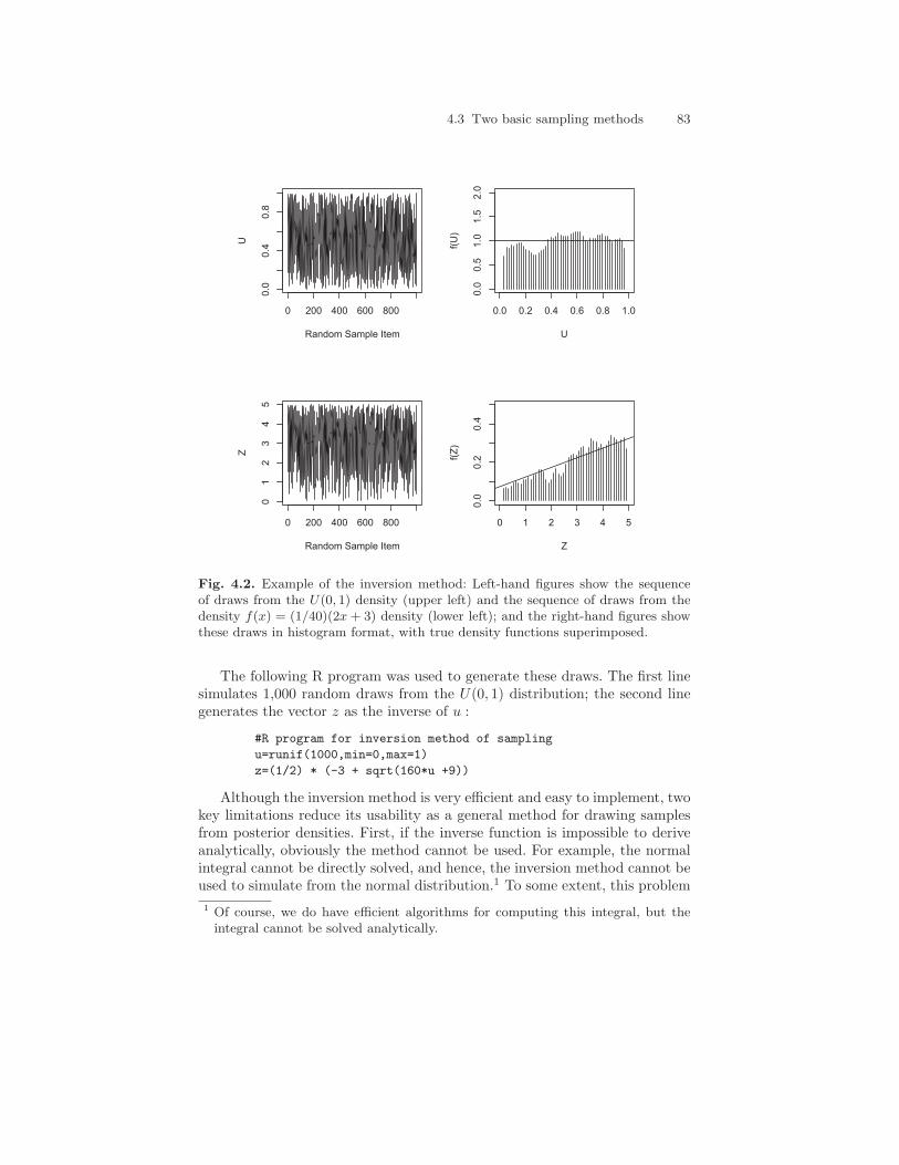
Figure 4.2 displays the results of an algorithm simulating 1,000 randomdraws from this density using the inversion method. The figures on the left-hand side show the sequence of draws from the U(0, 1) density, which arethen inverted to produce the sequence of draws from the density of interest.The right-hand side of the figure shows the simulated and theoretical densityfunctions. Notice how the samples from both densities closely follow, but donot exactly match, the theoretical densities. This error is sampling error, whichdiminishes as the simulation sample size increases.


0 200 400 600 800

0.0

0.4

0.8

Random Sample Item

U

0.0 0.2 0.4 0.6 0.8 1.0

0.0

0.5

1.0

1.5

2.0

U

f(U

)

0 200 400 600 800

01

23

45

Random Sample Item

Z

0 1 2 3 4 5

0.0

0.2

0.4

Z

f(Z

)

Fig. 4.2. Example of the inversion method: Left-hand figures show the sequenceof draws from the U(0, 1) density (upper left) and the sequence of draws from thedensity f(x) = (1/40)(2x + 3) density (lower left); and the right-hand figures showthese draws in histogram format, with true density functions superimposed.

The following R program was used to generate these draws. The first linesimulates 1,000 random draws from the U(0, 1) distribution; the second linegenerates the vector z as the inverse of u :

#R program for inversion method of sampling

u=runif(1000,min=0,max=1)

z=(1/2) * (-3 + sqrt(160*u +9))

Although the inversion method is very efficient and easy to implement, twokey limitations reduce its usability as a general method for drawing samplesfrom posterior densities. First, if the inverse function is impossible to deriveanalytically, obviously the method cannot be used. For example, the normalintegral cannot be directly solved, and hence, the inversion method cannot beused to simulate from the normal distribution.1 To some extent, this problem

1 Of course, we do have efficient algorithms for computing this integral, but theintegral cannot be solved analytically.


begs the question: If we can integrate the density as required by the inversionmethod, then why bother with simulation? This question will be addressedshortly, but the short answer is that we may not be able to perform integrationon a multivariate density, but we can often break a multivariate density intounivariate ones for which inversion may work.

The second problem with the inversion method is that the method willnot work with multivariate distributions, because the inverse is generally notunique beyond one dimension. For example, consider the bivariate planar den-sity function discussed in Chapter 2:

f(x, y) =1

28(2x + 3y + 2),

with 0 < x, y < 2. If we draw u ∼ U(0, 1) and attempt to solve the doubleintegral for x and y, we get:

28u = yx2 +3xy2

2+ 2xy,

which, of course, has infinitely many solutions (one equation with two un-knowns). Thinking ahead, we could select a value for one variable and thenuse the inversion method to draw from the conditional distribution of theother variable. This process would reduce the problem to one of samplingfrom univariate conditional distributions, which is the basic idea of Gibbssampling, as I discuss shortly.

4.3.2 The rejection method of sampling

When F−1(u) cannot be computed, other methods of sampling exist. A veryimportant one is rejection sampling. In rejection sampling, sampling from adistribution f(x) for x involves three basic steps:

1. Sample a value z from a distribution g(x) from which sampling is easyand for which values of m× g(x) are greater than f(x) at all points (m isa constant).

2. Compute the ratio R = f(z)m×g(z) .

3. Sample u ∼ U(0, 1). If R > u, then accept z as a draw from f(x). Other-wise, return to step 1.

In this algorithm, m×g(x) is called an “envelope function,” because of therequirement that the density function g(x) multiplied by some constant m begreater than the density function value for the distribution of interest [f(x)]at the same point for all points. In other words, m × g(x) envelops f(x). Instep 1, we sample a point z from the pdf g(x).

In step 2, we compute the ratio of the envelope function [m × g(x)] eval-uated at z to the density function of interest [f(x)] evaluated at the samepoint.


Finally, in step 3, we draw a U(0, 1) random variable u and compare itwith R. If R > u, then we treat the draw as a draw from f(x). If not, wereject z as coming from f(x), and we repeat the process until we obtain asatisfactory draw.

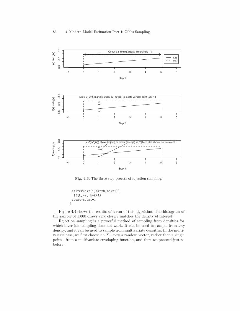
This routine is easy to implement, but it is not immediately apparent whyit works. Let’s again examine the density discussed in the previous section andconsider an envelope function that is a uniform density on the [0, 5] intervalmultiplied by a constant of 2. I choose this constant because the height ofthe U(0, 5) density is .2, whereas the maximum height of the density f(x) =(1/40)(2x + 3) is .325. Multiplying the U(0, 5) density by two increases theheight of this density to .4, which is well above the maximum for f(x) andtherefore makes m × g(x) a true envelope function. Figure 4.3 shows thedensity and envelope functions and graphically depicts the process of rejectionsampling.

In the first step, when we are sampling from the envelope function, we arechoosing a location on the x axis in the graph (see top graph in Figure 4.3).The process of constructing the ratio R and comparing it with a uniformdeviate is essentially a process of locating a point in the y direction oncethe x coordinate is chosen and then deciding whether it is under the densityof interest. This becomes more apparent if we rearrange the ratio and theinequality with u:

f(z) <=>︸︷︷︸

m× g(z)× u.

?

m × g(z) × u provides us a point in the y dimension that falls somewherebetween 0 and m× g(z). This can be easily seen by noting that m× g(z)× uis really simply providing a random draw from the U(0, g(z)) distribution:The value of this computation when u = 0 is 0; its value when u = 1 ism × g(z) (see middle graph in Figure 4.3). In the last step, in which wedecide whether to accept z as a draw from f(x), we are simply determiningwhether the y coordinate falls below the f(x) curve (see bottom graph inFigure 4.3). Another way to think about this process is that the ratio tells usthe proportion of times we will accept a draw at a given value of x as comingfrom the density of interest.

The following R program simulates 1,000 draws from the density f(x) =(1/40)(2x+3) using rejection sampling. The routine also keeps a count of howmany total draws from g(x) must be made in order to obtain 1,000 draws fromf(x).

#R program for rejection method of sampling

count=0; k=1; f=matrix(NA,1000)

while(k<1001)

{

z=runif(1,min=0,max=5)

r=((1/40)*(2*z+3))/(2*.2)


−1 0 1 2 3 4 5 6

0.0

0.3

0.6

Step 1

f(x)

and g

(x) Choose z from g(x) [say this point is '*']

f(x)

g(x)

−1 0 1 2 3 4 5 6

0.0

0.3

0.6

Step 2

f(x)

and g

(x) Draw u~U(0,1) and multiply by m*g(z) to locate vertical point [say '*']

−1 0 1 2 3 4 5 6

0.0

0.3

0.6

Step 3

f(x)

and g

(x) Is u*(m*g(z)) above (reject) or below (accept) f(z)? [here, it is above, so we reject]

Fig. 4.3. The three-step process of rejection sampling.

if(r>runif(1,min=0,max=1))

{f[k]=z; k=k+1}

count=count+1

}

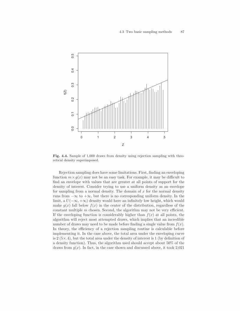
Figure 4.4 shows the results of a run of this algorithm. The histogram ofthe sample of 1,000 draws very closely matches the density of interest.

Rejection sampling is a powerful method of sampling from densities forwhich inversion sampling does not work. It can be used to sample from any

density, and it can be used to sample from multivariate densities. In the multi-variate case, we first choose an X—now a random vector, rather than a singlepoint—from a multivariate enveloping function, and then we proceed just asbefore.


0 1 2 3 4 5

0.0

0.1

0.2

0.3

0.4

0.5

Z

f(Z

)

Fig. 4.4. Sample of 1,000 draws from density using rejection sampling with theo-retical density superimposed.

Rejection sampling does have some limitations. First, finding an envelopingfunction m×g(x) may not be an easy task. For example, it may be difficult tofind an envelope with values that are greater at all points of support for thedensity of interest. Consider trying to use a uniform density as an envelopefor sampling from a normal density. The domain of x for the normal densityruns from −∞ to +∞, but there is no corresponding uniform density. In thelimit, a U(−∞,+∞) density would have an infinitely low height, which wouldmake g(x) fall below f(x) in the center of the distribution, regardless of theconstant multiple m chosen. Second, the algorithm may not be very efficient.If the enveloping function is considerably higher than f(x) at all points, thealgorithm will reject most attempted draws, which implies that an incrediblenumber of draws may need to be made before finding a single value from f(x).In theory, the efficiency of a rejection sampling routine is calculable beforeimplementing it. In the case above, the total area under the enveloping curveis 2 (5×.4), but the total area under the density of interest is 1 (by definition ofa density function). Thus, the algorithm used should accept about 50% of thedraws from g(x). In fact, in the case shown and discussed above, it took 2,021


attempts to obtain 1,000 draws from f(x), which is a rejection rate of 50.5%.These two limitations make rejection sampling, although possible, increasinglydifficult as the dimensionality increases in multivariate distributions.

4.4 Introduction to MCMC sampling

The limitations of inversion and rejection sampling make the prospects ofusing these simple methods daunting in complex statistical analyses involv-ing high-dimensional distributions. Although rejection sampling approachescan be refined to be more efficient, they are still not very useful in and ofthemselves in real-world statistical modeling. Fortunately, over the last fewdecades, MCMC methods have been developed that facilitate sampling fromcomplex distributions. Furthermore, aside from allowing sampling from com-plex distributions, these methods provide several additional benefits, as wewill be discussing in the remaining chapters.

MCMC sampling provides a method to sample from multivariate densitiesthat are not easy to sample from, often by breaking these densities downinto more manageable univariate or multivariate densities. The basic MCMCapproach provides a prescription for (1) sampling from one or more dimensionsof a posterior distribution and (2) moving throughout the entire support of aposterior distribution. In fact, the name “Markov chain Monte Carlo” impliesthis process. The “Monte Carlo” portion refers to the random simulationprocess. The “Markov chain” portion refers to the process of sampling a newvalue from the posterior distribution, given the previous value: This iterativeprocess produces a Markov chain of values that constitute a sample of drawsfrom the posterior.

4.4.1 Generic Gibbs sampling

The Gibbs sampler is the most basic MCMC method used in Bayesian statis-tics. Although Gibbs sampling was developed and used in physics prior to1990, its widespread use in Bayesian statistics originated in 1990 with its in-troduction by Gelfand and Smith (1990). As will be discussed more in the nextchapter, the Gibbs sampler is a special case of the more general Metropolis-Hastings algorithm that is useful when (1) sampling from a multivariate pos-terior is not feasible, but (2) sampling from the conditional distributions foreach parameter (or blocks of them) is feasible. A generic Gibbs sampler followsthe following iterative process (j indexes the iteration count):

4.4 Introduction to MCMC sampling 89

0. Assign a vector of starting values, S, to the parameter vector:Θj=0 = S.

1. Set j = j + 1.

2. Sample (θj1 | θj−1

2 , θj−13 . . . θj−1

k ).

3. Sample (θj2 | θj

1, θj−13 . . . θj−1

k )....

...

k. Sample (θjk | θ

j1, θj

2, . . . , θjk−1).

k+1. Return to step 1.

In other words, Gibbs sampling involves ordering the parameters and samplingfrom the conditional distribution for each parameter given the current value ofall the other parameters and repeatedly cycling through this updating process.Each “loop” through these steps is called an “iteration” of the Gibbs sampler,and when a new sampled value of a parameter is obtained, it is called an“updated” value.

For Gibbs sampling, the full conditional density for a parameter needs onlyto be known up to a normalizing constant. As we discussed in Chapters 2 and3, this implies that we can use the joint density with the other parametersset at their current values. This fact makes Gibbs sampling relatively simplefor most problems in which the joint density reduces to known forms for eachparameter once all other parameters are treated as fixed.

4.4.2 Gibbs sampling example using the inversion method

Here, I provide a simple example of Gibbs sampling based on the bivariateplane distribution developed in Chapter 2 f(x, y) = (1/28)(2x + 3y + 2). Theconditional distribution for x was:

f(x | y) =f(x, y)

f(y)=

2x + 3y + 2

6y + 8,

and the conditional distribution for y was:

f(y | x) =f(x, y)

f(x)=

2x + 3y + 2

4x + 10.

Thus, a Gibbs sampler for sampling x and y in this problem would followthese steps:

1. Set j = 0 and establish starting values. Here, let’s set xj=0 = −5 andyj=0 = −5.

2. Sample xj+1 from f(x | y = yj).3. Sample yj+1 from f(y | x = xj+1).4. Increment j = j + 1 and return to step 2 until j = 2000.


How do we sample from these conditional distributions? We know what theyare, but they certainly are not standard distributions. Since they are notstandard distributions, but since these conditionals are univariate and F−1()can be calculated for each one, we can use an inversion subroutine to samplefrom each conditional density. How do we find the inverses in this bivariatedensity? Recall that inversion sampling requires first drawing a u ∼ U(0, 1)random variable and then inverting this draw using F−1. Thus, to find theinverse of the conditional density for y|x, we need to solve:

u =

∫ z

0

2x + 3y + 2

4x + 10

for z. Given that this is the conditional density for y, x is fixed and can betreated as a constant, and we obtain:

u(4x + 10) = (2x + 2)y + (3/2)y2∣∣z

0.

Thus:

u(4x + 10) = (2x + 2)z + (3/2)z2.

After multiplying through by (2/3) and rearranging terms, we get:

(2/3)u(4x + 10) = z2 + (2/3)(2x + 2)z.

We can then complete the square in z and solve for z to obtain:

z =

√

(2/3)u(4x + 10) + ((1/3)(2x + 2))2 − (1/3)(2x + 2).

Given a current value for x and a random draw u, z is a random draw fromthe conditional density for y|x. A similar process can be undertaken to findthe inverse for x|y (see Exercises).

Below is an R program that implements the Gibbs sampling:

#R program for Gibbs sampling using inversion method

x=matrix(-5,2000); y=matrix(-5,2000)

for(i in 2:2000)

{

#sample from x | y

u=runif(1,min=0, max=1)

x[i]=sqrt(u*(6*y[i-1]+8)+(1.5*y[i-1]+1)*(1.5*y[i-1]+1))

-(1.5*y[i-1]+1)

#sample from y | x


y[i]=sqrt((2*u*(4*x[i]+10))/3 +((2*x[i]+2)/3)*((2*x[i]+2)/3))

- ((2*x[i]+2)/3)

}


This program first sets the starting values for x and y equal to −5. Then,x is updated using the current value of y. Then, y is updated using the just-sampled value of x. (Notice how x[i] is computed using y[i-1], whereasy[i] is sampled using x[i].) Both are updated using the inversion methodof sampling discussed above.

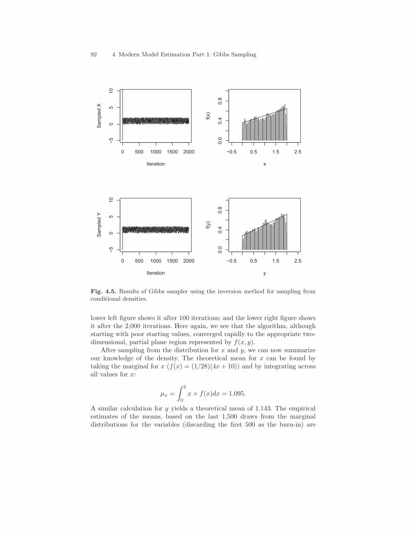
This algorithm produces samples from the marginal distributions for bothx and y, but we can also treat pairs of x and y as draws from the joint density.We will discuss the conditions in which we can do this in greater depth shortly.Generally, however, of particular interest are the marginal distributions forparameters, since we are often concerned with testing hypotheses concerningone parameter, net of the other parameters in a model. Figure 4.5 shows a“trace plot” of both x and y as well as the marginal densities for both variables.The trace plot is simply a two-dimensional plot in which the x axis representsthe iteration of the algorithm, and the y axis represents the simulated valueof the random variable at each particular iteration. Heuristically, we can thentake the trace plot, turn it on its edge (a 90 degree clockwise turn), and allowthe “ink” to fall down along the y-axis and “pile-up” to produce a histogramof the marginal density. Places in the trace plot that are particularly darkrepresent regions of the density in which the algorithm simulated frequently;lighter areas are regions of the density that were more rarely visited by thealgorithm. Thus, the “ink” will pile-up higher in areas for which the variableof interest has greater probability. Histograms of these marginal densities areshown to the right of their respective trace plots, with the theoretical marginaldensities derived in Chapter 2 superimposed. Realize that these marginals areunnormalized, because the leading 1/28 normalizing constant cancels in boththe numerator and the denominator.

Notice that, although the starting values were very poor (−5 is not a validpoint in either dimension of the density), the algorithm converged very rapidlyto the appropriate region—[0, 2]. It generally takes a number of iterations foran MCMC algorithm to find the appropriate region—and, more theoretically,for the Markov chain produced by the algorithm to sample from the appro-priate “target” distribution. Thus, we generally discard a number of earlyiterations before making calculations (called the “burn-in”). The marginaldensities, therefore, are produced from only the last 1,500 iterations of thealgorithm.

The histograms for the marginal densities show that the algorithm samplesappropriately from the densities of interest. Of course, there is certainly someerror—observe how the histograms tend to be a little too low or high hereand there. This reflects sampling error, and such error is reduced by samplingmore values (e.g., using 5,000 draws, rather than 2,000); we will return to thisissue in the next chapter.

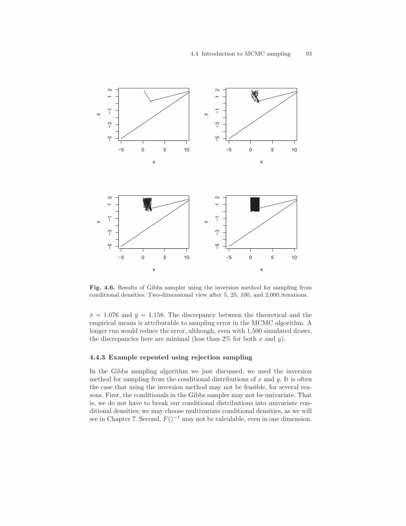
Aside from examining the marginal distributions for x and y, we can alsoexamine the joint density. Figure 4.6 shows a two-dimensional trace plot, takenat several stages. The upper left figure shows the state of the algorithm after5 iterations; the upper right figure shows the state after 25 iterations; the


0 500 1000 1500 2000

−5

05

10

Iteration

Sam

ple

d X

−0.5 0.5 1.5 2.5

0.0

0.4

0.8

x

f(x)

0 500 1000 1500 2000

−5

05

10

Iteration

Sam

ple

d Y

−0.5 0.5 1.5 2.5

0.0

0.4

0.8

y

f(y)

Fig. 4.5. Results of Gibbs sampler using the inversion method for sampling fromconditional densities.

lower left figure shows it after 100 iterations; and the lower right figure showsit after the 2,000 iterations. Here again, we see that the algorithm, althoughstarting with poor starting values, converged rapidly to the appropriate two-dimensional, partial plane region represented by f(x, y).

After sampling from the distribution for x and y, we can now summarizeour knowledge of the density. The theoretical mean for x can be found bytaking the marginal for x (f(x) = (1/28)(4x + 10)) and by integrating acrossall values for x:

µx =

∫ 2

0

x× f(x)dx = 1.095.

A similar calculation for y yields a theoretical mean of 1.143. The empiricalestimates of the means, based on the last 1,500 draws from the marginaldistributions for the variables (discarding the first 500 as the burn-in) are


−5 0 5 10

−5

−3

−1

12

x

y

−5 0 5 10

−5

−3

−1

12

x

y

−5 0 5 10

−5

−3

−1

12

x

y

−5 0 5 10

−5

−3

−1

12

x

y

Fig. 4.6. Results of Gibbs sampler using the inversion method for sampling fromconditional densities: Two-dimensional view after 5, 25, 100, and 2,000 iterations.

x = 1.076 and y = 1.158. The discrepancy between the theoretical and theempirical means is attributable to sampling error in the MCMC algorithm. Alonger run would reduce the error, although, even with 1,500 simulated draws,the discrepancies here are minimal (less than 2% for both x and y).

4.4.3 Example repeated using rejection sampling

In the Gibbs sampling algorithm we just discussed, we used the inversionmethod for sampling from the conditional distributions of x and y. It is oftenthe case that using the inversion method may not be feasible, for several rea-sons. First, the conditionals in the Gibbs sampler may not be univariate. Thatis, we do not have to break our conditional distributions into univariate con-ditional densities; we may choose multivariate conditional densities, as we willsee in Chapter 7. Second, F ()−1 may not be calculable, even in one dimension.


For example, if the distribution were bivariate normal, the conditionals wouldbe univariate normal, and F ()−1 cannot be analytically computed.2 Third,even if the inverse of the density is calculable, the normalizing constant in theconditional may not be easily computable. The inversion algorithm technicallyrequires the complete computation of F ()−1, which, in this case, requires us toknow both the numerator and the denominator of the formulas for the condi-tional distributions. It is often the case that we do not know the exact formulafor a conditional distribution, but instead, we know the conditional only upto a normalizing (proportionality) constant. Generally speaking, conditionaldistributions are proportional to the joint distribution evaluated at the pointof conditioning. So, for example, in the example discussed above, if we knowy = q, then the following is true:

f(x | y = q) = (1/28)× 2x + 3q + 2

6q + 8∝ 2x + 3q + 2.

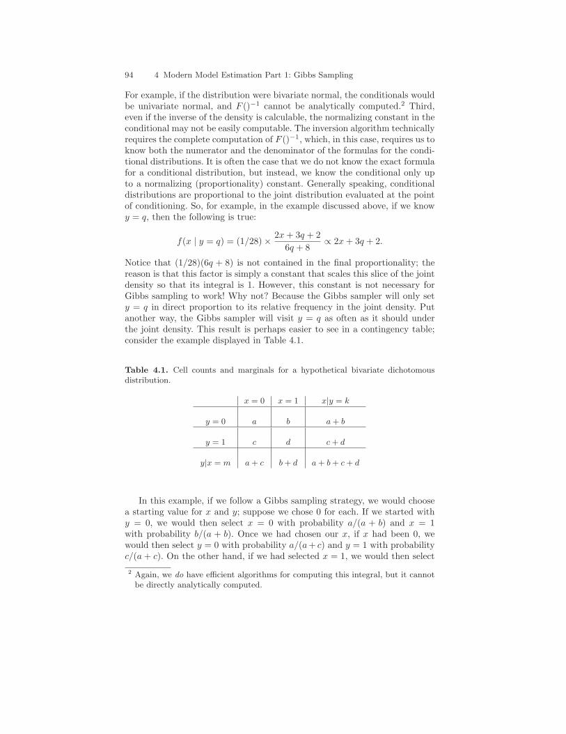
Notice that (1/28)(6q + 8) is not contained in the final proportionality; thereason is that this factor is simply a constant that scales this slice of the jointdensity so that its integral is 1. However, this constant is not necessary forGibbs sampling to work! Why not? Because the Gibbs sampler will only sety = q in direct proportion to its relative frequency in the joint density. Putanother way, the Gibbs sampler will visit y = q as often as it should underthe joint density. This result is perhaps easier to see in a contingency table;consider the example displayed in Table 4.1.

Table 4.1. Cell counts and marginals for a hypothetical bivariate dichotomousdistribution.

x = 0 x = 1 x|y = k

y = 0 a b a + b

y = 1 c d c + d

y|x = m a + c b + d a + b + c + d

In this example, if we follow a Gibbs sampling strategy, we would choosea starting value for x and y; suppose we chose 0 for each. If we started withy = 0, we would then select x = 0 with probability a/(a + b) and x = 1with probability b/(a + b). Once we had chosen our x, if x had been 0, wewould then select y = 0 with probability a/(a+ c) and y = 1 with probabilityc/(a + c). On the other hand, if we had selected x = 1, we would then select

2 Again, we do have efficient algorithms for computing this integral, but it cannotbe directly analytically computed.


y = 0 with probability b/(b + d) and y = 1 with probability d/(b + d). Thus,we would be selecting y = 0 with total probability

p(y = 0) = p(y = 0 | x = 0)p(x = 0) + p(y = 0 | x = 1)p(x = 1).

So,

p(y = 0) =

(a

a + c

)(a + c

a + b + c + d

)

+

(b

b + d

)(b + d

a + b + c + d

)

=a + b

a + b + c + d.

This proportion reflects exactly how often we should choose y = 0, giventhe marginal distribution for y in the contingency table. Thus, the normalizingconstant is not relevant, because the Gibbs sampler will visit each value ofone variable in proportion to its relative marginal frequency, which leads us tothen sample the other variable, conditional on the first, with the appropriaterelative marginal frequency.

Returning to the example at hand, then, we simply need to know whatthe conditional distribution is proportional to in order to sample from it.Here, if we know y = q, then f(x | y = q) ∝ 2x + 3q + 2. Because we do notnecessarily always know this normalizing constant, using the inversion methodof sampling will not work.3 However, we can simulate from this density usingrejection sampling. Recall from the discussion of rejection sampling that weneed an enveloping function g(x) that, when multiplied by a constant m,returns a value that is greater than f(x) for all x. With an unnormalizeddensity, only m must be adjusted relative to what it would be under thenormalized density in order to ensure this rule is followed. In this case, if wewill be sampling from the joint density, we can use a uniform density on the[0, 2] interval multiplied by a constant m that ensures that the density doesnot exceed m × .5 (.5 is the height of the U(0,2) density). The joint densityreaches a maximum where x and y are both 2; that peak value is 12. Thus,if we set m = 25, the U(0, 2) density multiplied by m will always be abovethe joint density. And, we can ignore the normalizing constants, includingthe leading (1/28) in the joint density and the 1/(6y + 8) in the conditionalfor x and the 1/(4x + 10) in the conditional for y. As exemplified above, theGibbs sampler will sample from the marginals in the correct proportion totheir relative frequency in the joint density. Below is a Gibbs sampler thatsimulates from f(x, y) using rejection sampling:

3 The normalizing constant must be known one way or another. Certainly, we canperform the integration we need to compute F−1 so long as the distribution isproper. However, if we do not know the normalizing constant, the integral willdiffer from 1, which necessitates that our uniform draw representing the areaunder the curve be scaled by the inverse of the normalizing constant in order torepresent the area under the unnormalized density fully.


#R program for Gibbs sampling using rejection sampling

x=matrix(-1,2000); y=matrix(-1,2000)

for(i in 2:2000)

{

#sample from x | y using rejection sampling

z=0

while(z==0)

{

u=runif(1,min=0, max=2)

if( ((2*u)+(3*y[i-1])+2) > (25*runif(1,min=0,max=1)*.5))

{x[i]=u; z=1}

}

#sample from y | x using rejection sampling

z=0

while(z==0)

{


if( ((2*x[i])+(3*u)+2) > (25*runif(1,min=0,max=1)*.5))

{y[i]=u; z=1}

}

}

In this program, the overall Gibbs sampling process is the same as for theinversion sampling approach; the only difference is that we are now using re-jection sampling to sample from the unnormalized conditional distributions.One consequence of switching sampling methods is that we have now had touse better starting values (−1 here versus −5 under inversion sampling). Thereason for this is that the algorithm will never get off the ground otherwise.Notice that the first item to be selected is x[2]. If y[1] is -5, the first condi-tional statement (if . . .) will never be true: The value on the left side of theexpression, ((2*u)+(3*y[i-1])+2), can never be positive, but the value onthe right, (25*runif(1,min=0,max=1)*.5), will always be positive. So, thealgorithm will “stick” in the first while loop.

Figures 4.7 and 4.8 are replications of the previous two figures producedunder rejection sampling. The overall results appear the same. For example,the mean for x under the rejection sampling approach was 1.085, and themean for y was 1.161, which are both very close to those obtained using theinversion method.

4.4.4 Gibbs sampling from a real bivariate density

The densities we examined in the examples above were very basic densities(linear and planar) and are seldom used in social science modeling. In thissection, I will discuss using Gibbs sampling to sample observations from adensity that is commonly used in social science research—the bivariate normaldensity. As discussed in Chapter 2, the bivariate normal density is a specialcase of the multivariate normal density in which the dimensionality of the


0 500 1000 1500 2000

−5

05

10

Iteration

Sam

ple

d X

−0.5 0.5 1.5 2.5

0.0

0.4

0.8

x

f(x)

0 500 1000 1500 2000

−5

05

10

Iteration

Sam

ple

d Y

−0.5 0.5 1.5 2.5

0.0

0.4

0.8

y

f(y)

Fig. 4.7. Results of Gibbs sampler using rejection sampling to sample from condi-tional densities.

density is 2, and the variables—say x and y—in this density are related bythe correlation parameter ρ. For the sake of this example, we will use thestandard bivariate normal density—that is, the means and variances of bothx and y are 0 and 1, respectively—and we will assume that ρ is a knownconstant (say, .5). The pdf in this case is:

f(x, y|ρ) =1

2π√

1− ρ2exp

{

−x2 − 2ρxy + y2

2(1− ρ2)

}

.

In order to use Gibbs sampling for sampling values of x and y, we need todetermine the full conditional distributions for both x and y, that is, f(x|y)and f(y|x). I have suppressed the conditioning on ρ in these densities, simplybecause ρ is a known constant in this problem.


−5 0 5 10

−5

−3

−1

12

x (after 5 iterations)

y

−5 0 5 10

−5

−3

−1

12


y

−5 0 5 10

−5

−3

−1

12


y

−5 0 5 10

−5

−3

−1

12


y

Fig. 4.8. Results of Gibbs sampler using rejection sampling to sample from condi-tional densities: Two-dimensional view after 5, 25, 100, and 2,000 iterations.

As we discussed above, Gibbs sampling does not require that we knowthe normalizing constant; we only need to know to what density each con-ditional density is proportional. Thus, we will drop the leading constant(1/(2π

√

1− ρ2)). The conditional for x then requires that we treat y asknown. If y is known, we can reexpress the kernel of the density as

f(x|y) ∝ exp

{

−x2 − x(2ρy)

2(1− ρ2)

}

exp

{

− y2

2(1− ρ2)

}

,

and we can drop the latter exponential containing y2, because it is simply aproportionality constant with respect to x. Thus, we are left with the left-handexponential. If we complete the square in x, we obtain

f(x|y) ∝ exp

{

− (x2 − x(2ρy) + (ρy)2 − (ρy)2)

2(1− ρ2)

}

,


which reduces to

f(x|y) ∝ exp

{

− (x− ρy)2 − (ρy)2

2(1− ρ2)

}

.

Given that both ρ and y are constants in the conditional for x, the latter termon the right in the numerator can be extracted just as y2 was above, and weare left with:

f(x|y) ∝ exp

{

− (x− ρy)2

2(1− ρ2)

}

.

Thus, the full conditional for x can be seen as proportional to a univariatenormal density with a mean of ρy and a variance of (1− ρ2). We can find thefull conditional for y exactly the same way. By symmetry, the full conditionalfor y will be proportional to a univariate normal density with a mean of ρxand the same variance.

Writing a Gibbs sampler to sample from this bivariate density, then, isquite easy, especially given that R (and most languages) have efficient algo-rithms for sampling from normal distributions (rnorm in R). Below is an Rprogram that does such sampling:

#R program for Gibbs sampling from a bivariate normal pdf

x=matrix(-10,2000); y=matrix(-10,2000)

for(j in 2:2000)

{

#sampling from x|y

x[j]=rnorm(1,mean=(.5*y[j-1]),sd=sqrt(1-.5*.5))

#sampling from y|x

y[j]=rnorm(1,mean=(.5*x[j]),sd=sqrt(1-.5*.5))

}

This algorithm is quite similar to the Gibbs sampler shown previously forthe bivariate planar density. The key difference is that the conditionals arenormal; thus, x and y are updated using the rnorm random sampling function.

Figure 4.9 shows the state of the algorithm after 10, 50, 200, and 2,000iterations. As the figure shows, despite the poor starting values of −10 for bothx and y, the algorithm rapidly converged to the appropriate region (within10 iterations).

Figure 4.10 contains four graphs. The upper graphs show the marginaldistributions for x and y for the last 1,500 iterations of the algorithm, withthe appropriate “true” marginal distributions superimposed. As these graphsshow, the Gibbs sampler appears to have generated samples from the appro-priate marginals. In fact, the mean and standard deviation for x are .059 and.984, respectively, which are close to their true values of 0 and 1. Similarly, themean and standard deviation for y were .012 and .979, which are also close totheir true values.


−10 −6 −2 0 2 4

−10

−6

−2

24


y

−10 −6 −2 0 2 4

−10

−6

−2

24


y

−10 −6 −2 0 2 4

−10

−6

−2

24


y

−10 −6 −2 0 2 4

−10

−6

−2

24


y

Fig. 4.9. Results of Gibbs sampler for standard bivariate normal distribution withcorrelation r = .5: Two-dimensional view after 10, 50, 200, and 2,000 iterations.

As I said earlier, we are typically interested in just the marginal distri-butions. However, I also stated that the samples of x and y can also beconsidered—after a sufficient number of burn-in iterations—as a sample fromthe joint density for both variables. Is this true? The lower left graph in thefigure shows a contour plot for the true standard bivariate normal distributionwith correlation r = .5. The lower right graph shows this same contour plotwith the Gibbs samples superimposed. As the figure shows, the countour plotis completely covered by the Gibbs samples.

4.4.5 Reversing the process: Sampling the parameters given the data

Sampling data from densities, conditional on the parameters of the density,as we did in the previous section is an important process, but the process ofBayesian statistics is about sampling parameters conditional on having data,


−4 −2 0 2 4

0.0

0.2

0.4

x

f(x)

−4 −2 0 2 4

0.0

0.2

0.4

y

f(y)

x

y

−4 −2 0 2 4

−4

−2

02

4

x

y

−4 −2 0 2 4

−4

−2

02

4

Fig. 4.10. Results of Gibbs sampler for standard bivariate normal distribution:Upper left and right graphs show marginal distributions for x and y (last 1,500iterations); lower left graph shows contour plot of true density; and lower rightgraph shows contour plot of true density with Gibbs samples superimposed.

not about sampling data conditional on knowing the parameters. As I haverepeatedly said, however, from the Bayesian perspective, both data and pa-rameters are considered random quantities, and so sampling the parametersconditional on data is not a fundamentally different process than samplingdata conditional on parameters. The main difference is simply in the mathe-matics we need to apply to the density to express it as a conditional densityfor the parameters rather than for the data. We first saw this process in theprevious chapter when deriving the conditional posterior distribution for themean parameter from a univariate normal distribution.

Let’s first consider a univariate normal distribution example. In the pre-vious chapter, we derived two results for the posterior distributions for themean and variance parameters (assuming a reference prior of 1/σ2). In one, weshowed that the posterior density could be factored to produce (1) a marginalposterior density for σ2 that was an inverse gamma distribution, and (2) aconditional posterior density for µ that was a normal distribution:


p(σ2|X) ∝ IG ((n− 1)/2 , (n− 1)var(x)/2)

p(µ|σ2, X) ∝ N(x , σ2/n

).

In the second derivation for the posterior distribution for σ2, we showedthat the conditional (not marginal) distribution for σ2 was also an inversegamma distribution, but with slightly different parameters:

p(σ2|µ,X) ∝ IG(

n/2 ,∑

(xi − µ)2/2)

.

Both of these derivations lend themselves easily to Gibbs sampling. Underthe first derivation, we could first sample a vector of values for σ2 from themarginal distribution and then sample a value for µ conditional on each valueof σ2 from its conditional distribution. Under the second derivation, we wouldfollow the iterative process shown in the previous sections, first sampling avalue for σ2 conditional on µ, then sampling a value for µ conditional on thenew value for σ2, and so on.

In practice, the first approach is more efficient. However, some situationsmay warrant the latter approach (e.g., when missing data are included). Here,I show both approaches in estimating the average years of schooling for theadult U.S. population in 2000. The data for this example are from the 2000National Health Interview Survey (NHIS), a repeated cross-sectional surveyconducted annually since 1969. The data set is relatively large by social sciencestandards, consisting of roughly 40,000 respondents in each of many years. In2000, after limiting the data to respondents 30 years and older and deletingobservations missing on education, I obtained an analytic sample of 17,946respondents. Mean educational attainment in the sample was 12.69 years (s.d.= 3.16 years), slightly below the mean of 12.74 from the 2000 U.S. Census.4

Below is an R program that first samples 2,000 values of the variance ofeducational attainment (σ2) from its inverse gamma marginal distributionand then, conditional on each value for σ2, samples µ from the appropriatenormal distribution:

#R: sampling from marginal for variance and conditional for mean

x<-as.matrix(read.table("c:\\education.dat",header=F)[,1])

sig<-rgamma(2000,(length(x)-1)/2 , rate=((length(x)-1)*var(x)/2))

sig<-1/sig

mu<-rnorm(2000,mean=mean(x),sd=(sqrt(sig/length(x))))

4 In calculating the mean from the census, I recoded the census categories for (1)under 9 years; (2) 9-12 years, no diploma; (3) high-school graduate or equivalent;(4) some college, no degree; (5) Associate degree; (6) Bachelor degree; and (4)graduate or professional degree to the midpoint for years of schooling and createda ceiling of 17 years, which is the upper limit for the NHIS.

4.5 Conclusions 103

This program is remarkably short, first reading the data into a vector Xand then generating 2,000 draws from a gamma distribution with the appro-priate shape and scale parameters. These draws are then inverted, because Rhas no direct inverse gamma distribution; thus, I make use of the fact that, if1/x is gamma distributed with parameters a and b, then x is inverse gammadistributed with the same parameters. Finally, the program samples µ fromits appropriate normal distribution.

Below is the R program for the alternative approach in which µ and σ aresequentially sampled from their conditional distributions:

#R: sampling from conditionals for both variance and mean

x<-as.matrix(read.table("c:\\education.dat",header=F)[,1])

mu=matrix(0,2000); sig=matrix(1,2000)

for(i in 2:2000)

{

sig[i]=rgamma(1,(length(x)/2),rate=sum((x-mu[i-1])^2)/2)

sig[i]=1/sig[i]

mu[i]=rnorm(1,mean=mean(x),sd=sqrt(sig[i]/length(x)))

}

Under this approach, we must select starting values for µ and σ2; here Iuse 0 and 1, respectively (assigned when the matrices are defined in R), whichare far from their estimates based on the sample means. This approach alsonecessitates looping, as we saw in the planar density earlier.

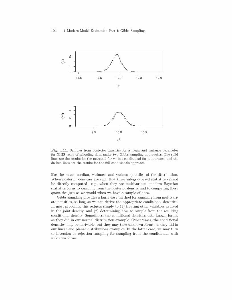
Figure 4.11 shows the results of both algorithms. The first 1,000 draws havebeen discarded from each run, because the poor starting values in the secondalgorithm imply that convergence is not immediate. In contrast, under thefirst method, convergence is immediate; the first 1,000 are discarded simplyto have comparable sample sizes. As the figure shows, the results are virtuallyidentical for the two approaches.

Numerically, the posterior means for µ under the two approaches were both12.69, and the posterior means for σ2 were 10.01 and 10.00, respectively (the

means for√

σ2 were both 3.16). These results are virtually identical to thesample estimates of these parameters, as they should be. A remaining questionmay be: What are the reasonable values for mean education in the population?In order to answer this question, we can construct a 95% “empirical probability

interval” for µ by taking the 25th and 975th sorted values of µ from ourGibbs samples. For both approaches, the resulting interval is [12.64 , 12.73],which implies that the true population mean for years of schooling falls in thisinterval with probability .95.

4.5 Conclusions

As we have seen in the last two chapters, the Bayesian approach to inferenceinvolves simply summarizing the posterior density using basic sample statistics


12.5 12.6 12.7 12.8 12.9

05

15

µ

f(µ)

9.5 10.0 10.5

02

4

σ2

f(σ

2)

Fig. 4.11. Samples from posterior densities for a mean and variance parameterfor NHIS years of schooling data under two Gibbs sampling approaches: The solidlines are the results for the marginal-for-σ2-but conditional-for-µ approach; and thedashed lines are the results for the full conditionals approach.

like the mean, median, variance, and various quantiles of the distribution.When posterior densities are such that these integral-based statistics cannotbe directly computed—e.g., when they are multivariate—modern Bayesianstatistics turns to sampling from the posterior density and to computing thesequantities just as we would when we have a sample of data.

Gibbs sampling provides a fairly easy method for sampling from multivari-ate densities, so long as we can derive the appropriate conditional densities.In most problems, this reduces simply to (1) treating other variables as fixedin the joint density, and (2) determining how to sample from the resultingconditional density. Sometimes, the conditional densities take known forms,as they did in our normal distribution example. Other times, the conditionaldensities may be derivable, but they may take unknown forms, as they did inour linear and planar distributions examples. In the latter case, we may turnto inversion or rejection sampling for sampling from the conditionals withunknown forms.

4.6 Exercises 105

In some cases, however, inversion of a conditional density may not be pos-sible, and rejection sampling may be difficult or very inefficient. In those cases,Bayesians can turn to another method—the Metropolis-Hastings algorithm.Discussion of that method is the topic of the next chapter. For alternative andmore in-depth and theoretical expositions of the Gibbs sampler, I recommendthe entirety of Gilks, Richardson, and Spiegelhalter 1996 in general and Gilks1996 in particular. I also recommend a number of additional readings in theconcluding chapter of this book.

4.6 Exercises

1. Find the inverse distribution function (F−1) for y|x in the bivariate planardensity; that is, show how a U(0, 1) sample must be transformed to be adraw from y|x.

2. Develop a rejection sampler for sampling data from the bivariate planardensity f(x) ∝ 2x + 3y + 2.

3. Develop an inversion sampler for sampling data from the linear densityf(x) ∝ 5x + 2. (Hint: First, find the normalizing constant, and then findthe inverse function).

4. Develop an appropriate routine for sampling the λ parameter from thePoisson distribution voting example in the previous chapter.

5. Develop an appropriate routine for sampling 20 observations (data points)from an N(0, 1) distribution. Then, reverse the process using these datato sample from the posterior distribution for µ and σ2. Use the noninfor-mative prior p(µ , σ2) ∝ 1/σ2, and use either Gibbs sampler describedin the chapter. Next, plot the posterior density for µ, and superimposean appropriate t distribution over this density. How close is the match?Discuss.

6. As we have seen throughout this chapter, computing integrals (e.g., themean and variance) using sampling methods yields estimates that are notexact in finite samples but that become better and better estimates as thesample size increases. Describe how we might quantify how much samplingerror is involved in estimating quantities using sampling methods (Hint:Consider the Central Limit Theorem).

4 modern model estimation part 1: gibbs samplingbrian/463-663/week10/chapter 04.pdf80 4 modern model...

Documents