4 monte carlo methods in classical statistical physics - institut für

4 Monte Carlo Methods in ClassicalStatistical Physics

Wolfhard Janke

Institut fur Theoretische Physik and Centre for Theoretical Sciences, Universitat Leipzig,04009 Leipzig, Germany

The purpose of this chapter is to give a brief introduction to Monte Carlo simu-lations of classical statistical physics systems and their statistical analysis. To setthe general theoretical frame, first some properties of phase transitions and sim-ple models describing them are briefly recalled, before the concept of importancesampling Monte Carlo methods is introduced. The basic idea is illustrated by a fewstandard local update algorithms (Metropolis, heat-bath, Glauber). Then methodsfor the statistical analysis of the thus generated data are discussed. Special atten-tion is payed to the choice of estimators, autocorrelation times and statistical erroranalysis. This is necessary for a quantitative description of the phenomenon of crit-ical slowing down at continuous phase transitions. For illustration purposes, onlythe two-dimensional Ising model will be needed. To overcome the slowing-downproblem, non-local cluster algorithms have been developed which will be describednext. Then the general tool of reweighting techniques will be explained which is ex-tremely important for finite-size scaling studies. This will be demonstrated in somedetail by the sample study presented in the next section, where also methods for es-timating spatial correlation functions will be discussed. The reweighting idea is alsoimportant for a deeper understanding of so-called generalized ensemble methodswhich may be viewed as dynamical reweighting algorithms. After first discussingsimulated and parallel tempering methods, finally also the alternative approach us-ing multicanonical ensembles and the Wang-Landau recursion are briefly outlined.

4.1 Introduction

Classical statistical physics is a well understood subject which poses, however,many difficult problems when a concrete solution for interacting systems is sought.In almost all non-trivial applications, analytical methods can only provide approxi-mate answers. Numerical computer simulations are, therefore, an important comple-mentary method on our way to a deeper understanding of complex physical systemssuch as (spin) glasses and disordered magnets or of biologically motivated prob-lems such as protein folding. Quantum statistical problems in condensed matter orthe broad field of elementary particle physics and quantum gravity are other ma-jor applications which, after suitable mappings, also rely on classical simulationtechniques.

W. Janke: Monte Carlo Methods in Classical Statistical Physics, Lect. Notes Phys. 739, 79–140 (2008)DOI 10.1007/978-3-540-74686-7 4 c© Springer-Verlag Berlin Heidelberg 2008

80 W. Janke

In these lecture notes we shall confine ourselves to a survey of computer simu-lations based on Markov chain Monte Carlo methods which realize the importancesampling idea. Still, not all aspects can be discussed in these notes in detail, and forfurther reading the reader is referred to recent textbooks [1, 2, 3, 4], where someof the material is presented in more depth. For illustration purposes, here we shallfocus on the simplest spin models, the Ising and Potts models. From a theoreticalpoint of view, also spin systems are still of current interest since they provide thepossibility to compare completely different approaches such as field theory, seriesexpansions, and simulations. They are also the ideal testing ground for general con-cepts such as universality, scaling or finite-size scaling, where even today some newfeatures can still be discovered. And last but not least, they have found a revival inslightly disguised form in quantum gravity and and random network theory, wherethey serve as idealized matter fields on Feynman diagrams or fluctuating graphs.

This chapter is organized as follows. In Sect. 4.2, first the definition of the stan-dard Ising model is recalled and the most important observables (specific heat, mag-netization, susceptibility, correlation functions, . . . ) are briefly discussed. Next somecharacteristic properties of phase transitions, their scaling properties, the definitionof critical exponents and finite-size scaling are briefly summarized. In Sect. 4.3,the basic method underlying all importance sampling Monte Carlo simulations isdescribed and some properties of local update algorithms (Metropolis, heat-bath,Glauber) are discussed. The following Sect. 4.4 is devoted to non-local cluster al-gorithms which in some cases can dramatically speed up the simulations. A fairlydetailed account of the initial non-equilibrium period and ageing phenomena as wellas statistical error analysis in equilibrium is given in Sect. 4.5. Here temporal corre-lation effects are discussed, which explain the problems with critical slowing downat a continuous phase transition and exponentially large flipping times at a first-order transition. In Sect. 4.6, we discuss reweighting techniques which are particu-larly important for finite-size scaling studies. A worked out example of such a studyis presented in the following Sect. 4.7. Finally, more refined generalized ensemblesimulation methods are briefly outlined in Sect. 4.8, focusing on simulated and par-allel tempering, the multicanonical ensemble and the Wang-Landau recursion. Thelecture notes close in Sect. 4.9 with a few concluding remarks.

4.2 Statistical Physics Primer

To set the scenery for the simulation methods discussed below, we need to brieflyrecall a few basic concepts of statistical physics [5, 6, 7, 8]. In these lecture noteswe will only consider classical systems and mainly focus on the canonical ensemblewhere the partition function is generically given as

Z =∑states

e−βH = e−βF , (4.1)

with the summation running over all possible states of the system. The state spacemay be continuous or discrete. As usual β ≡ 1/kBT denotes the inverse temperature

4 Monte Carlo Methods in Classical Statistical Physics 81

fixed by an external heat bath, kB is Boltzmann’s constant,H is the Hamiltonian ofthe system, encoding the details of the interactions which may be short-, medium-,or long-ranged, and F is the free energy. Expectation values denoted by angularbrackets 〈. . .〉 then follow as

〈O〉 =∑states

Oe−βH/Z , (4.2)

whereO stands symbolically for any observable, e.g., the energyE ≡ H.As we will see in the next section, the most elementary Monte Carlo simulation

method (Metropolis algorithm) can, in principle, cope with all conceivable variantsof this quite general formulation. Close to a phase transition, however, this basic al-gorithm tends to become very time consuming and for accurate quantitative resultsone needs to employ more refined methods. Most of them are much more specificand take advantage of certain properties of the model under study. One still quitebroad class of systems are lattice models, where one assumes that the degrees offreedom live on the sites or/and links of a D-dimensional lattice. These are oftentaken to be hypercubic, but more complicated regular lattice types (e.g., triangular(T), body-centered cubic (BCC), face-centered cubic (FCC), etc.) and even randomlattices do not cause problems in principle. The degrees of freedom may be continu-ous or discrete field variables such as a gauge field or the height variable of a crystalsurface, continuous or discrete spins such as the three-dimensional unit vectors ofthe classical Heisenberg model or the ±1 valued spins of the Ising model, or arrowconfigurations along the links of the lattice such as in Baxter’s vertex models, togive only a few popular examples.

To be specific and to keep the discussion as simple as possible, most simulationmethods will be illustrated with the minimalistic Ising model [9, 10] where

H = −J∑〈ij〉

σiσj − h∑i

σi (4.3)

with σi = ±1. Here J is a coupling constant which is positive for a ferromagnet(J > 0) and negative for an anti-ferromagnet (J < 0), h is an external magneticfield, and the symbol 〈ij〉 indicates that the lattice sum is restricted to run onlyover all nearest-neighbor pairs. In the examples discussed below, usually periodicboundary conditions are applied. And to ease the notation, we will always assumeunits in which kB = 1 and J = 1.

Basic observables are the internal energy per site, u = U/V , with U =−d lnZ/dβ ≡ 〈H〉, and the specific heat

C =dudT

= β2 〈E2〉 − 〈E〉2V

= β2V(〈e2〉 − 〈e〉2) , (4.4)

where we have set H ≡ E = eV with V denoting the number of lattice sites, i.e.,the lattice volume. The magnetization per site m = M/V and the susceptibility χare defined as

82 W. Janke

M =1β

d lnZdh

= V 〈μ〉 , μ =1V

∑i

σi , (4.5)

andχ = βV

(〈μ2〉 − 〈μ〉2) . (4.6)

The correlation between spins σi and σj at sites labeled by i and j can be measuredby considering correlation functions like the two-point spin-spin correlationG(i, j),which is defined as

G(r) = G(i, j) = 〈σiσj〉 − 〈σi〉〈σj〉 , (4.7)

where r = ri − rj (assuming translational invariance). Away from criticality andat large distances |r| � 1 (where we have assumed a lattice spacing a = 1), G(r)decays exponentially

G(r) ∼ |r|κ e−|r|/ξ , (4.8)

where ξ is the correlation length and the exponent κ of the power-law prefactordepends in general on the dimension and on whether one studies the ordered ordisordered phase. Some model (and simulation) specific details of the latter observ-ables and further important quantities like various magnetization cumulants will bediscussed later when dealing with concrete applications.

The Ising model is the paradigm model for systems exhibiting a continuous (or,roughly speaking, second-order) phase transition from an ordered low-temperatureto a disordered high-temperature phase at some critical temperature Tc when thetemperature is varied. In two dimensions (2D), the thermodynamic limit of thismodel in zero external field has been solved exactly by Onsager [11], and also forfinite Lx × Ly lattices the exact partition function is straightforward to compute[12, 13]. For infinite lattices, even the correlation length is known in arbitrary latticedirections [14, 15]. The exact magnetization for h = 0, apparently already knownto Onsager [16]1, was first derived by Yang [17, 18], and the susceptibility is knownto very high precision [19, 20], albeit still not exactly. In 3D no exact solutions areavailable, but analytical and numerical results from various methods give a consis-tent and very precise picture.

The most characteristic feature of a second-order phase transition is the diver-gence of the correlation length at Tc. As a consequence thermal fluctuations areequally important on all length scales, and one therefore expects power-law sin-gularities in thermodynamic functions. The leading divergence of the correlationlength is usually parameterized in the high-temperature phase as

ξ = ξ0+ |1− T/Tc|−ν + . . . (T ≥ Tc) , (4.9)

where the . . . indicate sub-leading analytical as well as confluent corrections. Thisdefines the critical exponent ν > 0 and the critical amplitude ξ0+ on the high-temperature side of the transition. In the low-temperature phase one expects a simi-lar behavior1 See also the historical remarks in Refs. [14, 15].


ξ = ξ0−(1− T/Tc)−ν + . . . (T ≤ Tc) , (4.10)

with the same critical exponent ν but a different critical amplitude ξ0− �= ξ0+ .An important consequence of the divergence of the correlation length is that

qualitative properties of second-order phase transitions should not depend on short-distance details of the Hamiltonian. This is the basis of the universality hypothesis[21] which means that all (short-ranged) systems with the same symmetries andsame dimensionality should exhibit similar singularities governed by one and thesame set of critical exponents. For the amplitudes this is not true, but certain ampli-tude ratios are also universal.

The singularities of the specific heat, magnetization (for T < Tc), and suscepti-bility are similarly parameterized by the critical exponents α, β and γ, respectively,

C = Creg + C0|1− T/Tc|−α + . . . ,

m = m0(1− T/Tc)β + . . . ,

χ = χ0|1− T/Tc|−γ + . . . , (4.11)

where Creg is a regular background term, and the amplitudes are again in generaldifferent on the two sides of the transition. Right at the critical temperature Tc, twofurther exponents δ and η are defined through

m ∝ h1/δ ,

G(r) ∝ r−D+2−η . (4.12)

In the 1960’s, Rushbrooke [22], Griffiths [23], Josephson [24, 25] and Fisher[26] showed that these six critical exponents are related via four inequalities. Sub-sequent experimental evidence indicated that these relations were in fact equalities,and they are now firmly established and fundamentally important in the theory ofcritical phenomena. With D representing the dimensionality of the system, the scal-ing relations are

Dν = 2− α (Josephson’s law) ,

2β + γ = 2− α (Rushbrooke’s law) ,

β(δ − 1) = γ (Griffiths’ law) ,

ν(2 − η) = γ (Fisher’s law) . (4.13)

In the conventional scaling scenario, Rushbrooke’s and Griffiths’ laws can be de-duced from the Widom scaling hypothesis that the Helmholtz free energy is a ho-mogeneous function [27, 28]. Widom scaling and the remaining two laws can in turnbe derived from the Kadanoff block-spin construction [29] and ultimately from thatof the renormalization group (RG) [30]. Josephson’s law can also be derived fromthe hyperscaling hypothesis, namely that the free energy behaves near criticality as

84 W. Janke

Table 4.1. Critical exponents of the Ising model in two (2D) and three (3D) dimensions. All2D exponents are exactly known [31, 32], while for the 3D Ising model the world-averagefor ν and γ calculated in [33] is quoted. The other exponents follow from the hyperscalingrelation α = 2 − Dν, and the scaling relations β = (2 − α − γ)/2, δ = γ/β + 1, andη = 2 − γ/ν

dimension ν α β γ δ η

D = 2 1 0 (log) 1/8 7/4 15 1/4

D = 3 0.630 05(18) 0.109 85 0.326 48 1.237 17(28) 4.7894 0.036 39

the inverse correlation volume: f∞(t) ∼ ξ−D∞ (t). Twice differentiating this relationone recovers Josephson’s law (4.13). The critical exponents for the 2D and 3D Isingmodel [31, 32, 33] are collected in Table 4.1.

In any numerical simulation study, the system size is necessarily finite. Whilethe correlation length may still become very large, it is therefore always finite. Thisimplies that also the divergences in other quantities are rounded and shifted [34, 35,36, 37]. How this happens is described by finite-size scaling (FSS) theory, which ina nut-shell may be explained as follows: Near Tc the role of ξ is taken over by thelinear size L of the system. By rewriting (4.9) or (4.10) and replacing ξ → L

|1− T/Tc| ∝ ξ−1/ν −→ L−1/ν , (4.14)

it is easy to see that the scaling laws (4.11) are replaced by the FSS Ansatze,

C = Creg + aLα/ν + . . . ,

m ∝ L−β/ν + . . . ,

χ ∝ Lγ/ν + . . . . (4.15)

As a mnemonic rule, a critical exponent x of the temperature scaling law isreplaced by −x/ν in the corresponding FSS law. In general these scaling laws arevalid in a neighborhood of Tc as long as the scaling variable

x = (1− T/Tc)L1/ν (4.16)

is kept fixed [34, 35, 36, 37]. This implies for the locations Tmax of the (finite)maxima of thermodynamic quantities such as the specific heat or susceptibility, anFSS behavior of the form

Tmax = Tc(1− xmaxL−1/ν + . . .) . (4.17)

In this more general formulation the scaling law for, e.g., the susceptibility reads

χ(T, L) = Lγ/νf(x) , (4.18)

where f(x) is a scaling function. By plotting χ(T, L)/Lγ/ν versus the scaling vari-able x, one thus expects that the data for different T and L fall onto a master


curve described by f(x). This is a nice visual method for demonstrating the scalingproperties.

Similar considerations for first-order phase transitions [38, 39, 40, 41] showthat here the δ-function like singularities in the thermodynamic limit, originatingfrom phase coexistence, are also smeared out for finite systems [42, 43, 44, 45,46]. They are replaced by narrow peaks whose height (width) grows proportional tothe volume (1/volume) with a displacement of the peak location from the infinite-volume limit proportional to 1/volume [47, 48, 49, 50, 51, 52].

4.3 The Monte Carlo Method

Let us now discuss how the expectation values in (4.2) can be estimated in a MonteCarlo simulation. For any reasonable system size, a direct summation of the parti-tion function is impossible, since already for the minimalistic Ising model with onlytwo possible states per site the number of terms would be enormous: For a moderate20×20 lattice, the state space consists already of 2400≈10120 different spin config-urations.2 Also a naive random sampling of the spin configurations does not work.Here the problem is that the relevant region in the high-dimensional phase space isrelatively narrow and hence too rarely hit by random sampling. The solution to thisproblem is known since long under the name importance sampling [53].

4.3.1 Importance Sampling

The basic idea of importance sampling is to set up a suitable Markov chain thatdraws configurations not at random but according to their Boltzmann weight

Peq({σi}) =e−βH({σi})

Z . (4.19)

A Markov chain defines stochastic rules for transitions from one state to anothersubject to the condition that the probability for the new configuration only dependson the preceding state but not on the history of the whole trajectory in state space,i.e., it is almost local in time. Symbolically this can be written as

. . .W−→ {σi} W−→ {σi}′ W−→ {σi}′′ W−→ . . . , (4.20)

where the transition probabilityW has to satisfy the following conditions:

(i) W ({σi} −→ {σi}′) ≥ 0 for all {σi}, {σi}′,(ii)

∑{σi}′ W ({σi} −→ {σi}′) = 1 for all {σi},

(iii)∑

{σi}W ({σi} −→ {σi}′)P eq({σi}) = P eq({σi}′) for all {σi}′.

2 This number should be compared with the estimated number of protons in the Universewhich is about 1080.

86 W. Janke

From condition (iii) we see that the desired Boltzmann distribution P eq is a fixedpoint of W (eigenvector of W with unit eigenvalue). A somewhat simpler sufficientcondition is detailed balance,

Peq({σi})W ({σi} −→ {σi}′) = Peq({σi}′)W ({σi}′ −→ {σi}) . (4.21)

By summing over {σi} and using condition (ii), the more general condition (iii)follows. After an initial equilibration period (cf. Sect. 4.5.1), expectation values canbe estimated as an arithmetic mean over the Markov chain of length N , e.g.,

E = 〈H〉 =∑{σi}H({σi})Peq({σi}) ≈ 1

N

N∑j=1

H({σi}j) , (4.22)

where {σi}j denotes the spin configuration at “time” j. A more detailed expositionof the mathematical concepts underlying any Markov chain Monte Carlo algorithmcan be found in many textbooks and reviews [1, 2, 3, 4, 34, 54, 55].

4.3.2 Local Update Algorithms

The Markov chain conditions (i)–(iii) are still quite general and can be satisfied bymany different concrete update rules. In a rough classification one distinguishes be-tween local and non-local algorithms. Local update algorithms discussed in thissubsection are conceptually much simpler and, as the main merit, quite univer-sally applicable. The main drawback is their relatively poor performance close tosecond-order phase transitions where the spins or fields of a typical configurationare strongly correlated over large spatial distances. Here non-local update algo-rithms based on multigrid methods or in particular self-adaptive cluster algorithmsdiscussed later in Sect. 4.4 perform much better.

4.3.2.1 Metropolis Algorithm

The most flexible update rule is the classic Metropolis algorithm [56], whichis applicable in practically all cases (lattice/off-lattice, discrete/continuous, short-range/long-range interactions, . . . ). Here one proposes an update for a single degreeof freedom (spin, field, . . . ) and accepts this proposal with probability

W ({σi}old −→ {σi}new) =

{1 Enew < Eold

e−β(Enew−Eold) Enew ≥ Eold, (4.23)

whereEold andEnew denote the energy of the old and new spin configuration {σi}old

and {σi}new, respectively, where {σi}new differs from {σi}old only locally by onemodified degree of freedom at, say, i = i0. More compactly, this may also be writ-ten as

W ({σi}old −→ {σi}new) = min{1, e−βΔE} , (4.24)


where ΔE = Enew − Eold. If the proposed update lowers the energy, it is alwaysaccepted. On the other hand, when the new configuration has a higher energy, the up-date has still to be accepted with a certain probability in order to ensure the propertreatment of entropic contributions – in thermal equilibrium, it is the free energyF = U − TS which has to be minimized and not the energy. Only in the limit ofzero temperature, β →∞, the acceptance probability for this case tends to zero andthe Metropolis method degenerates to a minimization algorithm for the energy func-tional. With some additional refinements, this is the basis for the simulated anneal-ing technique [57], which is often applied to hard optimization and minimizationproblems.

The verification of the detailed balance condition (4.21) is straightforward. IfEnew < Eold, then the l.h.s. of (4.21) becomes exp(−βEold) × 1 = exp(−βEold).On the r.h.s. we have to take into account that the reverse move would increasethe energy, Eold > Enew (with Eold now playing the role of the new energy), suchthat now the second line of (4.23) with Eold and Enew interchanged is relevant.This gives exp(−βEnew)× exp(−β(Eold − Enew)) = exp(−βEold) on the r.h.s. of(4.21), completing the demonstration of detailed balance. In the opposite case withEnew < Eold, a similar reasoning leads to exp(−βEold)× exp(−β(Enew−Eold)) =exp(−βEnew) = exp(−βEnew)× 1. Admittedly, this proof looks a bit like a tautol-ogy. To uncover its non-trivial content, it is a useful exercise to replace the r.h.s. ofthe Metropolis rule (4.23) by some general function f(Enew − Eold) and repeat theabove steps [58].

Finally a few remarks on the practical implementation of the Metropolis methodare in order. To decide whether a proposed update should be accepted or not, onedraws a uniformly distributed random number r ∈ [0, 1), and if W ≤ r, the newstate is accepted. Otherwise one keeps the old configuration and continues withthe next spin. In computer simulations, random numbers are generated by meansof pseudo-random number generators (RNGs), which produce (more or less) uni-formly distributed numbers whose values are very hard to predict – by using somedeterministic rule (see [59] and references therein). In other words, given a finitesequence of subsequent pseudo-random numbers, it should be (almost) impossibleto predict the next one or to even guess the deterministic rule underlying their gen-eration. The goodness of an RNG is thus measured by the difficulty to derive itsunderlying deterministic rule. Related requirements are the absence of trends (cor-relations) and a very long period. Furthermore, an RNG should be portable amongdifferent computer platforms and, very importantly, it should yield reproducible re-sults for testing purposes. The design of RNGs is a science in itself, and many thingscan go wrong with them. As a recommendation one should better not experimenttoo much with some fancy RNG one has picked up somewhere from the Web, say,but rely on well-tested and well-documented routines.

There are many different ways how the degrees of freedom to be updated canbe chosen. They may be picked at random or according to a random permutation,which can be updated every now and then. But also a simple fixed lexicographical

88 W. Janke

(sequential) order is permissible.3 In lattice models one may also update first all oddand then all even sites, which is the usual choice in vectorized codes. A so-calledsweep is completed when on the average4 for all degrees of freedom an update wasproposed. The qualitative behavior of the update algorithm is not sensitive to thesedetails, but its quantitative performance does depend on the choice of the updatescheme.

4.3.2.2 Heat-Bath Algorithm

This algorithm is only applicable to lattice models and at least in its most straight-forward form only to discrete degrees of freedom with a few allowed states. Thenew value σ′

i0 at site i0 is determined by testing all its possible states in the heat-bath of its (fixed) neighbors (e.g., four on a square lattice and six on a simple-cubiclattice with nearest-neighbor interactions):

W ({σi}old −→ {σi}new) =e−βH({σi}new)∑σi0

e−βH({σi}old)=

e−βσ′i0Si0∑

σi0e−βσi0Si0

, (4.25)

where Si0 = −∑j σj − h is an effective spin or field collecting all neighboring

spins (in their old states) interacting with the spin at site i0 and h is the externalmagnetic field. Note that this decomposition also works in the case of vectors (σi →σi, h → h, Si0 → Si0 ), interacting via the usual dot product (σ′

i0Si0 → σ′

i0·

Si0). As the last equality in (4.25) shows, all other contributions to the energy notinvolving σ′

i0cancel due to the ratio in (4.25), so that for the update at each site i0

only a small number of computations is necessary (e.g, about four for a square andsix for a simple-cubic lattice of arbitrary size). Detailed balance (4.21) is obviouslysatisfied since

e−βH({σi}old)e−βH({σi}new)∑σi0

e−βH({σi}new)= e−βH({σi}new) e−βH({σi}old)∑

σi0e−βH({σi}old)

. (4.26)

How is the probability (4.25) realized in practice? Due to the summation overall local states, special tricks are necessary when each degree of freedom cantake many different states, and only in special cases the heat-bath method can beefficiently generalized to continuous degrees of freedom. In many applications,however, the admissible local states of σi0 can be labeled by a small number ofintegers, say n = 1, . . . , N . Since the probability in (4.25) is normalized to unity,the sequence (P1, P2, . . . , Pn, . . . , PN ) decomposes the unit interval into segmentsof length Pn = exp(−βnSi0)/

∑Nk=1 exp(−βkSi0). If one now draws a random

number R ∈ [0, 1) and compares the accumulated probabilities∑nk=1 Pk with R,

then the new state n0 is given as the smallest integer for which∑n0k=1 Pk ≥ R.

Clearly, for a large number of possible local states, the determination of n0 can be-come quite time-consuming (in particular, if many small Pn are at the beginning

3 Some special care is necessary, however, for one-dimensional spin chains.4 This is only relevant when the random update order is chosen.


of the sequence, in which case a clever permutation of the Pn-list can help a lot).The order of updating the individual variables can be chosen as for the Metropolisalgorithm (random, sequential, . . . ).

In the special case of the Ising model with only two states per spin, σi = ±1,(4.25) reads explicitly as

W ({σi}old −→ {σi}new) =e−βσ

′i0Si0

eβSi0 + e−βSi0. (4.27)

And since ΔE = Enew − Eold = (σ′i0− σi0 )Si0 , the probability for a spin flip,

σ′i0 = −σi0 , becomes [58]

Wσi0→−σi0=

e−βΔE/2

eβΔE/2 + e−βΔE/2. (4.28)

The acceptance ratio (4.28) is plotted in Fig. 4.1 as a function of ΔE for various(inverse) temperatures and compared with the corresponding ratio (4.24) of theMetropolis algorithm. As we shall see in the next paragraph, for the Ising model,the Glauber and heat-bath algorithm are identical.

4.3.2.3 Glauber Algorithm

The Glauber update prescription [60] is conceptually similar to the Metropolis algo-rithm in that also here a local update proposal is accepted with a certain probability

−8 −4 0 4 8energy difference ΔE

0.0

0.2

0.4

0.6

0.8

1.0

acce

ptan

ce r

atio

β = 0.2β = 0.44β = 1.0

M

HB

Fig. 4.1. Comparison of the acceptance ratio for a spin flip with the heat-bath (HB) (orGlauber) and Metropolis (M) algorithm in the Ising model for three different inverse temper-atures β. Note that for all values of ΔE and temperature, the Metropolis acceptance ratio ishigher than that of the heat-bath algorithm

90 W. Janke

or otherwise rejected. For the Ising model with spins σi = ±1 the acceptance prob-ability can be written as

Wσi0→−σi0=

12

[1 + σi0 tanh (βSi0)] , (4.29)

where as before σi0Si0 with Si0 = −∑j σj − h is the energy of the ith0 spin in the

current old state.Due to the point symmetry of the hyperbolic tangent, one may rewrite σi0 tanh

(βSi0) as tanh (σi0βSi0). And since as before ΔE = Enew − Eold = −2σi0Si0 ,(4.29) becomes

Wσi0→−σi0=

12

[1− tanh (βΔE/2)] , (4.30)

showing explicitly that the acceptance probability only depends on the total en-ergy change as in the Metropolis case. In this form it is thus possible to generalizethe Glauber update rule from the Ising model with only two states per spin to anygeneral model that can be simulated with the Metropolis procedure. Also detailedbalance is straightforward to prove. Finally by using trivial identities for hyperbolicfunctions, (4.30) can be further recast to read

Wσi0→−σi0=

12

[cosh(βΔE/2)− sinh(βΔE/2)

cosh(βΔE/2)

]

=e−βΔE/2

eβΔE/2 + e−βΔE/2, (4.31)

which is just the flip probability (4.28) of the heat-bath algorithm for the Isingmodel, i.e., heat-bath updates for the special case of a 2-state model and the Glauberupdate algorithm are identical. In the general case with more than two states perspin, however, this is not the case.

The Glauber (or equivalently heat-bath) update algorithm for the Ising model isalso theoretically of interest since in this case the dynamics of the Markov chain canbe calculated analytically for a one-dimensional system [60]. For two and higherdimensions, however, no exact solutions are known.

4.3.3 Performance of Local Update Algorithms

Local update algorithms are applicable to a very wide class of models and the com-puter codes are usually quite simple and very fast. The main drawback are tempo-ral correlations of the generated Markov chain which tend to become huge in thevicinity of phase transitions. They can be determined by analysis of autocorrelationfunctions

A(k) =〈OiOi+k〉 − 〈Oi〉〈Oi〉〈O2

i 〉 − 〈Oi〉〈Oi〉, (4.32)

whereO denotes any measurable quantity, for example the energy or magnetization.More details and how temporal correlations enter into the statistical error analysis


will be discussed in Sect. 4.5.2.3. For large time separations k, A(k) decays expo-nentially (a = const)

A(k) k→∞−−−−→ ae−k/τO,exp , (4.33)

which defines the exponential autocorrelation time τO,exp. At smaller distances usu-ally also other modes contribute and A(k) behaves no longer purely exponentially.

This is illustrated in Fig. 4.2 for the 2D Ising model on a rather small 16×16square lattice with periodic boundary conditions at the infinite-volume critical pointβc = ln(1 +

√2)/2 = 0.440 686 793 . . .. The spins were updated in sequential

order by proposing always to flip a spin and accepting or rejecting this proposalaccording to (4.23). The raw data of the simulation are collected in a time-seriesfile, storing 1 000 000 measurements of the energy and magnetization taken aftereach sweep over the lattice, after discarding (quite generously) the first 200 000sweeps for equilibrating the system from a disordered start configuration. The last1 000 sweeps of the time evolution of the energy are shown in Fig. 4.2(a). Using thecomplete time series the autocorrelation function was computed according to (4.32)which is shown in Fig. 4.2(b). On the linear-log scale of the inset we clearly see theasymptotic linear behavior of lnA(k). A linear fit of the form (4.33), lnA(k) =ln a − k/τe,exp, in the range 10 ≤ k ≤ 40 yields an estimate for the exponentialautocorrelation time of τe,exp ≈ 11.3. In the small k behavior of A(k) we observean initial fast drop, corresponding to faster relaxing modes, before the asymptoticbehavior sets in. This is the generic behavior of autocorrelation functions in realisticmodels where the small-k deviations are, in fact, often much more pronounced thanfor the 2D Ising model.

Close to a critical point, in the infinite-volume limit, the autocorrelation timetypically scales as

τO,exp ∝ ξz , (4.34)

where z ≥ 0 is the so-called dynamical critical exponent. Since the spatial correla-tion length ξ ∝ |T−Tc|−ν →∞when T → Tc, also the autocorrelation time τO,exp

Fig. 4.2. (a) Part of the time evolution of the energy e = E/V for the 2D Ising model ona 16×16 lattice at βc = ln(1 +

√2)/2 = 0.440 686 793 . . . and (b) the resulting autocor-

relation function. In the inset the same data are plotted on a logarithmic scale, revealing afast initial drop for very small k and noisy behavior for large k. The solid lines show a fitto the ansatz A(k) = a exp(−k/τe,exp) in the range 10 ≤ k ≤ 40 with τe,exp = 11.3 anda = 0.432

92 W. Janke

diverges when the critical point is approached, τO,exp ∝ |T − Tc|−νz . This leads tothe phenomenon of critical slowing down at a continuous phase transition. This isnot in the first place a numerical artefact, but can also be observed experimentally forinstance in critical opalescence, see Fig. 1.1 in [5]. The reason is that local spin-flipMonte Carlo dynamics (or diffusion dynamics in a lattice-gas picture) describes atleast qualitatively the true physical dynamics of a system in contact with a heat-bath(which, in principle, enters stochastic elements also in molecular dynamics simula-tions). In a finite system, the correlation length ξ is limited by the linear system sizeL, and similar to the reasoning in (4.14) and (4.15), the scaling law (4.34) becomes

τO,exp ∝ Lz . (4.35)

For local dynamics, the critical slowing down effect is quite pronounced sincethe dynamical critical exponent takes a rather large value around

z ≈ 2 , (4.36)

which is only weakly dependent on the dimensionality and can be understood by asimple random-walk or diffusion argument in energy space. Non-local update algo-rithms such as multigrid schemes or in particular the cluster methods discussed inthe next section can reduce the value of the dynamical critical exponent z signifi-cantly, albeit in a strongly model-dependent fashion.

At a first-order phase transition, a completely different mechanism leads to aneven more severe slowing-down problem [47]. Here, the password is phase coex-istence. A finite system close to the (pseudo-) transition point can flip between thecoexisting pure phases by crossing a two-phase region. Relative to the weight of thepure phases, this region of state space is strongly suppressed by an additional Boltz-mann factor exp(−2σLd−1), where σ denotes the interface tension between thecoexisting phases, Ld−1 is the (projected) area of the interface and the factor twoaccounts for periodic boundary conditions, which enforce always an even numberof interfaces for simple topological reasons. The time spent for crossing this highlysuppressed rare-event region scales proportional to the inverse of this interfacialBoltzmann factor, implying that the autocorrelation time increases exponentiallywith the system size,

τO,exp ∝ e2σLd−1. (4.37)

In the literature, this behavior is sometimes termed supercritical slowing down, eventhough, strictly speaking, nothing is critical at a first-order phase transition. Sincethis type of slowing-down problem is directly related to the shape of the probabilitydistribution, it appears for all types of update algorithms, i.e., in contrast to thesituation at a second-order transition, here it cannot be cured by employing multigridor cluster techniques. It can be overcome, however, at least in part by means oftempering and multicanonical methods also briefly discussed at the end of thesenotes in Sect. 4.8.


4.4 Cluster Algorithms

In this section we first concentrate on the problem of critical slowing down at asecond-order phase transition which is caused by very large spatial correlations, re-flecting that excitations become equally important on all length scales. It is thereforeintuitively clear that some sort of non-local updates should be able to alleviate thisproblem. While it was realized since long that whole clusters or droplets of spinsshould play a central role in such an update, it took until 1987 before Swendsenand Wang [61] proposed a legitimate cluster update procedure first for q-state Pottsmodels [62] with

HPotts = −J∑〈ij〉

δσi,σj , (4.38)

where σi = 1, . . . , q. For q = 2 (and a trivial rescaling) the Ising model (4.3)is recovered. Soon after this discovery, Wolff [63] introduced the so-called single-cluster variant and developed a generalization to O(n)-symmetric spin models. Bynow cluster update algorithms have been constructed for many other models as well[64]. However, since in all constructions some model specific properties enter in acrucial way, they are still far less general applicable than local update algorithms ofthe Metropolis type. We therefore first concentrate again on the Ising model where(as for more general Potts models) the prescription for a cluster-update algorithmcan be easily read off from the equivalent Fortuin-Kasteleyn representation [65, 66,67, 68]

Z =∑{σi}

eβ∑

〈ij〉 σiσj (4.39)

=∑{σi}

∏〈ij〉

eβ[(1− p) + pδσi,σj

](4.40)

=∑{σi}

∑{nij}

∏〈ij〉

eβ[(1 − p)δnij ,0 + pδσi,σjδnij ,1

](4.41)

withp = 1− e−2β . (4.42)

Here the nij are bond occupation variables which can take the values nij = 0 ornij = 1, interpreted as deleted or active bonds. The representation (4.40) in thesecond line follows from the observation that the product σiσj of two Ising spinscan only take the two values ±1, so that exp(βσiσj) = x + yδσiσj can easily besolved for x and y. And in the third line (4.41) we made use of the trivial (but clever)identity a+ b =

∑1n=0 (aδn,0 + bδn,1).

4.4.1 Swendsen-Wang Cluster

According to (4.41) a cluster update sweep consists of two alternating steps. First,updates of the bond variables nij for given spins, and second updates of the spinsσi for a given bond configuration. In practice one proceeds as follows:

94 W. Janke

always

Fig. 4.3. Illustration of the bond variable update. The bond between unlike spins is alwaysdeleted as indicated by the dashed line. A bond between like spins is only active with prob-ability p = 1 − exp(−2β). Only at zero temperature (β → ∞) stochastic and geometricalclusters coincide

(i) Set nij = 0 if σi �= σj , or assign values nij = 1 and 0 with probability p and1− p, respectively, if σi = σj , cp. Fig. 4.3.

(ii) Identify clusters of spins that are connected by active bonds (nij = 1).(iii) Draw a random value ±1 independently for each cluster (including one-site

clusters), which is then assigned to all spins in a cluster.

Technically the cluster identification part is the most complicated step, but thereare by now quite a few efficient algorithms available which can even be used onparallel computers. Vectorization, on the other hand, is only partially possible.

Notice the difference between the just defined stochastic clusters and geometri-cal clusters whose boundaries are defined by drawing lines through bonds betweenunlike spins. In fact, since in the stochastic cluster definition also bonds betweenlike spins are deleted with probability p0 = 1 − p = exp(−2β), stochastic clus-ters are smaller than geometrical clusters. Only at zero temperature (β → ∞) p0

approaches zero and the two cluster definitions coincide.As described above, the cluster algorithm is referred to as Swendsen-Wang (SW)

or multiple-cluster update [61]. The distinguishing point is that the whole lattice isdecomposed into stochastic clusters whose spins are assigned a random value +1 or−1. In one sweep one thus attempts to update all spins of the lattice.

4.4.2 Wolff Cluster

Shortly after the original discovery of cluster algorithms, Wolff [63] proposed asomewhat simpler variant in which only a single cluster is flipped at a time. Thisvariant is therefore sometimes also called single-cluster algorithm. Here one choosesa lattice site at random, constructs only the cluster connected with this site, and thenflips all spins of this cluster. In principle, one could also here choose for all spins inthe updated cluster a new value +1 or −1 at random, but then nothing at all wouldbe changed if one hits the current value of the spins. Typical configuration plotsbefore and after the cluster flip are shown in Fig. 4.4, which also nicely illustrates thedifference between stochastic and geometrical clusters already stressed in the lastparagraph. The upper right plot clearly shows that, due to the randomly distributedinactive bonds between like spins, the stochastic cluster is much smaller than theunderlying black geometrical cluster which connects all neighboring like spins.


Fig. 4.4. Illustration of the Wolff cluster update, using actual simulation results for the 2DIsing model at 0.97βc on a 100×100 lattice. Upper left: Initial configuration. Upper right:The stochastic cluster is marked. Note how it is embedded in the larger geometric clusterconnecting all neighboring like (black) spins. Lower left: Final configuration after flippingthe spins in the cluster. Lower right: The flipped cluster

In the single-cluster variant some care is necessary with the definition of the unitof time since the number of flipped spins varies from cluster to cluster. It also de-pends crucially on temperature since the average cluster size automatically adaptsto the correlation length. With 〈|C|〉 denoting the average cluster size, a sweep isusually defined to consist of V/〈|C|〉 single cluster steps, assuring that on the av-erage V spins are flipped in one sweep. With this definition, autocorrelation timesare directly comparable with results from the Swendsen-Wang or Metropolis algo-rithm. Apart from being somewhat easier to program, Wolff’s single-cluster variantis usually even more efficient than the Swendsen-Wang multiple-cluster algorithm,especially in 3D. The reason is that with the single-cluster method, on the average,larger clusters are flipped.

96 W. Janke

4.4.3 Embedded Clusters

While it is straightforward to generalize the derivation (4.39)–(4.42) to q-state Pottsmodels (because as in the Ising model each contribution to the energy, δσiσj , cantake only two different values), for O(n) spin models with Hamiltonian

H = −J∑〈ij〉

σi · σj , (4.43)

with σi = (σi,1, σi,2, . . . , σi,n) and |σi| = 1, one needs a new strategy for n ≥ 2[63, 69, 70, 71] (the case n = 1 degenerates again to the Ising model). Here thebasic idea is to isolate Ising degrees of freedom by projecting the spins σi onto arandomly chosen unit vector r

σi = σ‖i + σ⊥

i ,

σ‖i = ε |σi · r| r ,ε = sign(σi · r) . (4.44)

If this is inserted in the original Hamiltonian one ends up with an effectiveHamiltonian

H = −∑〈ij〉

Jijεiεj + const , (4.45)

with positive random couplings Jij = J |σi · r||σj · r| ≥ 0, whose Ising degrees offreedom εi can be updated with a cluster algorithm as described above.

4.4.4 Performance of Cluster Algorithms

The advantage of cluster algorithms is most pronounced close to criticality whereexcitations on all length scales occur. A convenient performance measure is thusthe dynamical critical exponent z (even though one should always check that theproportionality constant in τ ∝ Lz is not exceedingly large, but this is definitely notthe case here [72]). Some results on z are collected in Table 4.2, which allow us toconclude:

(i) Compared to local algorithms with z ≈ 2, z is dramatically reduced for bothcluster variants in 2D and 3D [73, 74, 75].

(ii) In 2D, Swendsen-Wang and Wolff cluster updates are equally efficient, whilein 3D, the Wolff update is clearly favorable.

(iii) In 2D, the scaling with system size can hardly be distinguished from a veryweak logarithmic scaling. Note that this is consistent with the Li-Sokal bound[76, 77] for the Swendsen-Wang cluster algorithm of τSW ≥ C ( = C0 +A lnLfor the 2D Ising model), implying zSW ≥ α/ν ( = 0 for the 2D Ising model).

(iv) Different observables (e.g., energy E and magnetization M ) may yield quitedifferent values for z when defined via the scaling behavior of the integratedautocorrelation time discussed below in Sect. 4.5.2.3.


Table 4.2. Dynamical critical exponents z for the 2D and 3D Ising model (τ ∝ Lz). The sub-scripts indicate the observables and method used (exp resp. int: exponential resp. integratedautocorrelation time, rel: relaxation, dam: damage spreading)

algorithm 2D 3D observable authors

Metropolis 2.1667(5) – zM,exp Nightingale andBlote [78, 79]

– 2.032(4) zdam Grassberger[80, 81]

– 2.055(10) zM,rel Ito et al. [82]

Swendsen-Wang cluster 0.35(1) 0.75(1) zE,exp Swendsen andWang [61]

0.27(2) 0.50(3) zE,int Wolff [72]

0.20(2) 0.50(3) zχ,int Wolff [72]

0(log L) – zM,exp Heermann andBurkitt [83]

0.25(5) – zM,rel Tamayo [84]

Wolff cluster 0.26(2) 0.28(2) zE,int Wolff [72]

0.13(2) 0.14(2) zχ,int Wolff [72]

0.25(5) 0.3(1) zE,rel Ito and Kohring[85]

4.4.5 Improved Estimators

The intimate relationship of cluster algorithms with the correlated percolation rep-resentation of Fortuin and Kasteleyn leads to another quite important improvementwhich is not directly related with the dynamical properties discussed so far. Withinthe percolation picture, it is quite natural to introduce alternative estimators (mea-surement prescriptions) for most standard quantities which turn out to be so-calledimproved estimators. By this one means measurement prescriptions that yield thesame expectation value as the standard ones but have a smaller statistical variancewhich helps to reduce the statistical errors. Suppose we want to measure the expec-tation value 〈O〉 of an observable O. Then any estimator O satisfying 〈O〉 = 〈O〉is permissible. This does not determine O uniquely since there are infinitely manyother possible choices O′ = O + X , as long as the added estimator X has zeroexpectation 〈X 〉 = 0. The variance of the estimator O′, however, can be quite dif-ferent and is not necessarily related to any physical quantity (contrary to the standardmean-value estimator of the energy, for instance, whose variance is proportional tothe specific heat). It is exactly this freedom in the choice of O which allows theconstruction of improved estimators.

For the single-cluster algorithm an improved cluster estimator for the spin-spincorrelation function in the high-temperature phaseG(xi−xj) ≡ 〈σi ·σj〉 is givenby [71]

98 W. Janke

G(xi − xj) = nV

|C| (r · σi) (r · σj) ΘC(xi)ΘC(xj) , (4.46)

where r is the normal of the mirror plane used in the construction of the cluster ofsize |C| and ΘC(x) is its characteristic function (= 1 if x ∈ C and zero otherwise).In the Ising case (n = 1), this simplifies to

G(xi − xj) =V

|C|ΘC(xi)ΘC(xj) , (4.47)

i.e., to the test whether the two sites xi and xj belong to same stochastic clusteror not. Only in the former case, the average over clusters is incremented by one,otherwise nothing is added. This implies that G(xi − xj) is strictly positive whichis not the case for the standard estimator σi · σj , where ±1 contributions have toaverage to a positive value. It is therefore at least intuitively clear that the cluster(or percolation) estimator has a smaller variance and is thus indeed an improvedestimator, in particular for large separations |xi − xj |.

For the Fourier transform G(k) =∑

xG(x) exp(−ik · x), (4.46) implies theimproved estimator

G(k) =

n

|C|

⎡⎣(∑i∈C

r · σi coskxi

)2

+

(∑i∈C

r · σi sin kxi

)2⎤⎦ , (4.48)

which, for k = 0, reduces to an improved estimator for the susceptibility χ′ =βV 〈m2〉 in the high-temperature phase

G(0) = χ′/β =

n

|C|

(∑i∈C

r · σi)2

. (4.49)

For the Ising model (n = 1) this reduces to χ′/β = 〈|C|〉, i.e., the improved estima-tor of the susceptibility is just the average cluster size of the single-cluster updatealgorithm. For the XY (n = 2) and Heisenberg (n = 3) model one finds empiricallythat in two as well as in three dimensions 〈|C|〉 ≈ 0.81χ′/β for n = 2 [69, 86] and〈|C|〉 ≈ 0.75χ′/β for n = 3 [71, 87], respectively.

Close to criticality, the average cluster size becomes large, growing ∝ χ′ ∝Lγ/ν � L2 (since γ/ν = 2 − η with η usually small) and the advantage of clusterestimators diminishes. In fact, in particular for short-range quantities such as theenergy (the next-neighbor correlation) it may even degenerate into a depraved ordeteriorated estimator, while long-range quantities such as G(xi − xj) for largedistances |xi−xj | usually still profit from it. A significant reduction of variance bymeans of the estimators (4.46)–(4.49) can, however, always be expected outside theFSS region where the average cluster size is small compared to the volume of thesystem.

Finally it is worth pointing out that at least for 2D Potts models also the geo-metrical clusters do encode critical properties – albeit those of different but related(tricritical) models [88, 89, 90, 91, 92]5.5 See also the extensive list of references to earlier work given therein.


4.5 Statistical Analysis of Monte Carlo Data

4.5.1 Initial Non-Equilibrium Period and Ageing

When introducing the importance sampling technique in Sect. 4.3.1 it was alreadyindicated in (4.22) that within Markov chain Monte Carlo simulations, the expec-tation value 〈O〉 of some quantity O, for instance the energy, can be estimated asarithmetic mean

〈O〉 =∑{σi}O({σi})P eq({σi}) ≈ O =

1N

N∑j=1

Oj , (4.50)

where Oj = O({σi}j) is the measured value for the jth configuration and N isthe number of measurement sweeps. Also a warning was given that this is onlyvalid after a sufficiently long equilibration period without measurements, which isneeded by the system to approach equilibrium after starting the Markov chain in anarbitrary initial configuration.

This initial equilibration or thermalization period, in general, is a non-trivialnon-equilibrium process which is of interest in its own right and no simple gen-eral recipe determining how long one should wait before starting measurementscan be given. Long suspected to be a consequence of the slow dynamics of glassysystems only, the phenomenon of ageing for example has also been found in thephase-ordering kinetics of simple ferromagnets such as the Ising model. To studythis effect numerically, one only needs the methods introduced so far since mosttheoretical concepts assume a local spin-flip dynamics as realized by one of thethree local update algorithms discussed above. Similarly to the concept of univer-sality classes in equilibrium, all three algorithms should yield qualitatively similarresults, being representatives of what is commonly referred to as dynamical Glauberuniversality class.

Let us assume that we pick as the initial configuration of the Markov chaina completely disordered state. If the simulation is run at a temperature T > Tc,equilibration will, in fact, be fast and nothing spectacular happens. If, however, wechoose instead to perform the simulation right at Tc or at a temperature T < Tc, thesituation is quite different. In the latter two cases one speaks of a quench, since nowthe starting configuration is in a statistical sense far away from a typical equilib-rium configuration at temperature T . This is easiest to understand for temperaturesT < Tc, where the typical equilibrium state consists of homogeneously ordered con-figurations. After the quench, local regions of parallel spins start forming domains orclusters, and the non-equilibrium dynamics of the system is governed by the move-ment of the domain walls. In order to minimize their surface energy, the domainsgrow and straighten their surface. A typical time evolution for the 2D Ising model isillustrated in Fig. 4.5, showing spin configurations after a quench to T < Tc, startingfrom an initially completely disordered state.

This leads to a growth law for the typical correlation length scale of the formξ ∼ t1/z , where t is the time (measured in units of sweeps) elapsed since the quench

100 W. Janke

Fig. 4.5. Phase-ordering with progressing Monte Carlo time (from left to right) of an initiallydisordered spin configuration for the 2D Ising model at T = 1.5 ≈ 0.66 Tc [93]

and z is the dynamical critical exponent already introduced in Sect. 4.3.2. In the caseof a simple ferromagnet like the Ising- or q-state Potts model with a non-conservedscalar order parameter, below Tc the dynamical exponent can be found exactly asz = 2 [94], according to diffusion or random-walk arguments. Right at the transitiontemperature, critical dynamics (for a recent review, see [95]) plays the central roleand the dynamical exponent of, e.g., the 2D Ising model takes the somewhat largernon-trivial value z ≈ 2.17 [78, 79] cf. Table 4.2. To equilibrate the whole system, ξmust approach the system size L, so that the typical relaxation time for equilibrationscales as

τrelax ∼ Lz . (4.51)

Note that this implies in the infinite-volume limit L→∞ that true equilibrium cannever be reached.

Since 1/z < 1, the relaxation process after the quench happens on a growingtime scale. This can be revealed most clearly by measurements of two-time quan-tities f(t, s) with t > s, which no longer transform time-translation invariantly asthey would do for small perturbations in equilibrium, where f would be a functionof the time difference t−s only. Instead, in phase-ordering kinetics, two-time quan-tities depend non-trivially on the ratio t/s of the two times. The dependence of therelaxation on the so-called waiting time s is the notional origin of ageing: Oldersamples respond more slowly.

For the most commonly considered two-time quantities, dynamical scalingforms can be theoretically predicted (for recent reviews see, e.g., [96, 97]). Wellstudied are the two-time autocorrelation function (here in q-state Potts modelnotation)

C(t, s) =1

q − 1

(q

V

V∑i=1

[δσi(t),σi(s)

]av− 1

)= s−bfC(t/s) , (4.52)

with the asymptotic behavior fC(x)→ x−λC/z (x� 1), and the two-time responsefunction

R(t, s) =δ [σi(t)]av

δhi(s)

∣∣∣∣h=0

= s−1−afR(t/s) , (4.53)

where fR(x) → x−λR/z (x � 1). Here h(s) is the amplitude of a small spa-tially random external field which is switched off after the waiting time s and [. . .]av


denotes an average over different random initial configurations (and random fieldsin (4.53)). In phase-ordering kinetics after a quench to T < Tc, in general b = 0 (andz = 2) [94], but all other exponents depend on the dimensionality of the consideredsystem. In the simplest case of the Ising model in two dimensions, it is commonlyaccepted that λC = λR = 5/4. The value of the remaining exponent a, however, ismore controversial [98, 99], with strong claims for a = 1/z = 1/2 [96, 100], butalso a = 1/4 [101, 102] has been conjectured. In computer simulation studies thetwo-time response function is rather difficult to handle and it is more convenient toconsider the integrated response or thermoremanent magnetization (TRM) [103],

ρ(t, s) = T

s∫0

duR(t, u) =T

hMTRM(t, s) . (4.54)

By extending dynamical scaling to local scale invariance (LSI) in analogy toconformal invariance [104], even explicit expressions of the scaling functions fC(x)and fR(x) have been predicted [105] (for a recent review, see [106]). For the 2Dand 3D Ising model, extensive numerical tests of the LSI predictions have beenperformed by Henkel, Pleimling and collaborators [107, 108, 109], showing a verygood agreement with the almost parameter-free analytical expressions. Recently thiscould be confirmed also for more general q-state Potts models with q = 3 and q = 8in two dimensions [93, 110].

If one is primarily interested in equilibrium properties of the considered statis-tical system, there is, of course, no need to study the initial equilibration periodin such a great detail. It is, however, advisable to watch the time evolution of thesystem and to make sure that no apparent trends are still visible when starting themeasurements. If estimates of the autocorrelation or relaxation time are available, agood a priori estimate is to wait at least about 20 τO,exp. Finally, as a (not furtherjustified) rule of thumb, most practicers of Monte Carlo simulations spend at leastabout 10% of the total computing time on the equilibration or thermalization period.

4.5.2 Statistical Errors and Autocorrelation Times

4.5.2.1 Estimators

As already indicated in (4.50), conceptually it is important to distinguish betweenthe expectation value 〈O〉 and the mean value O, which is an estimator for theformer. While 〈O〉 is an ordinary number and represents the exact result (which isusually unknown, of course), the estimator O is still a random number which forfinite N fluctuates around the theoretically expected value. Of course, from a singleMonte Carlo simulation with N measurements, we obtain only a single number forO at the end of the day. To estimate the statistical uncertainty due to the fluctuations,i.e., the statistical error bar, it seems at first sight that one would have to repeatthe whole simulation many times. Fortunately, this is not necessary since one canestimate the variance of O,

102 W. Janke

σ2O = 〈[O − 〈O〉]2〉 = 〈O2〉 − 〈O〉2 , (4.55)

from the statistical properties of individual measurements Oi, i = 1, . . . , N , in asingle Monte Carlo run.

4.5.2.2 Uncorrelated Measurements and Central-Limit Theorem

Inserting (4.50) into (4.55) gives

σ2O = 〈O2〉 − 〈O〉2 =

1N2

N∑i,j=1

〈OiOj〉 − 1N2

N∑i,j=1

〈Oi〉〈Oj〉 , (4.56)

and by collecting diagonal and off-diagonal terms one arrives at [111]

σ2O =

1N2

N∑i=1

(〈O2i 〉 − 〈Oi〉2

)+

1N2

N∑i�=j

(〈OiOj〉 − 〈Oi〉〈Oj〉) . (4.57)

Assuming equilibrium, the individual variances σ2Oi

= 〈O2i 〉 − 〈Oi〉2 do not de-

pend on “time” i, such that the first term gives σ2Oi/N . The second term with

〈OiOj〉 − 〈Oi〉〈Oj〉 = 〈(Oi − 〈Oi〉)(Oj − 〈Oj〉)〉 records the correlations be-tween measurements at times i and j. For completely uncorrelated data (which is,of course, an unrealistic assumption for importance sampling Monte Carlo simula-tions), the second term would vanish and (4.57) simplifies to

ε2O ≡ σ2O = σ2

Oi/N . (4.58)

This result is true for any distribution P(Oi). In particular, for the energy or mag-netization, distributions of the individual measurements are often plotted as phys-ically directly relevant (N independent) histograms (see, e.g., Fig. 4.8(b) below)whose squared width (= σ2

Oi) is proportional to the specific heat or susceptibility,

respectively.Whatever form the distribution P(Oi) assumes (which, in fact, is often close to

Gaussian because the Oi are usually already lattice averages over many degrees offreedom), by the central limit theorem the distribution of the mean value is Gaussian,at least for uncorrelated data in the asymptotic limit of large N . The variance ofthe mean, σ2

O , is the squared width of this (N dependent) distribution which isusually taken as the one-sigma squared error, ε2O ≡ σ2

O , and quoted together with

the mean value O. Under the assumption of a Gaussian distribution for the mean,the interpretation is that about 68% of all simulations under the same conditionswould yield a mean value in the range [O − σO,O + σO] [113]. For a two-sigmainterval which also is sometimes used, this percentage goes up to about 95.4%, andfor a three-sigma interval which is rarely quoted, the confidence level is higher than99.7%.


4.5.2.3 Correlated Measurements and Autocorrelation Times

For correlated data the second term in (4.57) does not vanish and things becomemore involved [114, 115, 116]. Using the symmetry i↔ j to reduce the summation∑Ni�=j to 2

∑Ni=1

∑Nj=i+1, reordering the summation, and using time-translation in-

variance in equilibrium, one finally obtains [111]

σ2O =

1N

[σ2Oi

+ 2N∑k=1

(〈O1O1+k〉 − 〈O1〉〈O1+k〉

)(1− k

N

)], (4.59)

where, due to the last factor (1− k/N), the k = N term may be trivially kept in thesummation. Factoring out σ2

Oi, this can be written as

ε2O ≡ σ2O =

σ2Oi

N2τ ′O,int , (4.60)

where we have introduced the (proper) integrated autocorrelation time

τ ′O,int =12

+N∑k=1

A(k)(

1− k

N

), (4.61)

with

A(k) ≡ 〈O1O1+k〉 − 〈O1〉〈O1+k〉σ2Oi

k→∞−−−−→ ae−k/τO,exp (4.62)

being the normalized autocorrelation function (A(0) = 1) already introduced in(4.32). Since in any meaningful simulation study N � τO,exp, A(k) in (4.61) isalready exponentially small before the correction term in parentheses becomes im-portant. For simplicity this correction is hence usually omitted (as is the prime ofτ ′O,int in (4.61)) and one employs the following definition for the integrated autocor-relation time

τO,int =12

+N∑k=1

A(k) . (4.63)

The notion “integrated” derives from the fact that this may be interpreted as a trape-zoidal discretization of the (approximate) integral τO,int ≈

∫ N0

dkA(k). Notice that,in general, τO,int (and also τ ′O,int) is different from τO,exp. In fact, one can show [117]that τO,int ≤ τO,exp in realistic models. Only if A(k) is a pure exponential, the twoautocorrelation times, τO,int and τO,exp, coincide (up to minor corrections for smallτO,int [58, 111]).

As far as the accuracy of Monte Carlo data is concerned, the important pointof (4.60) is that due to temporal correlations of the measurements the statistical

error εO ≡ O ⇒√σ2O on the Monte Carlo estimator O is enhanced by a factor

of√

2τO,int. This can be rephrased by writing the statistical error similar to the

uncorrelated case as εO =√σ2Oj/Neff, but now with a parameter

104 W. Janke

Neff = N/2τO,int ≤ N , (4.64)

describing the effective statistics. This shows more clearly that only every 2τO,int

iterations the measurements are approximately uncorrelated and gives a better ideaof the relevant effective size of the statistical sample. In view of the scaling behaviorof the autocorrelation time in (4.34), (4.35) or (4.37), it is obvious that without extracare this effective sample size may become very small close to a continuous or first-order phase transition, respectively.

4.5.2.4 Bias

A too small effective sample size does not only affect the error bars, but for somequantities even the mean values can be severely underestimated. This happens forso-called biased estimators, as is for instance the case for the specific heat andsusceptibility. The specific heat can be computed as C = β2V

(〈e2〉 − 〈e〉2) =β2V σ2

ei, with the standard estimator for the variance

σ2ei

= e2 − e2 = (e− e)2 =1N

N∑i=1

(ei − e)2 . (4.65)

Subtracting and adding 〈e〉2, one finds for the expectation value

〈σ2ei〉 = 〈e2 − e2〉 = (〈e2〉 − 〈e〉2)− (〈e2〉 − 〈e〉2) = σ2

ei+ σ2

e . (4.66)

Using (4.60) this gives

〈σ2ei〉 = σ2

ei

(1− 2τe,int

N

)= σ2

ei

(1− 1

Neff

)�= σ2

ei. (4.67)

The estimator σ2ei

in (4.65) thus systematically underestimates the true value by aterm of the order of τe,int/N . Such an estimator is called weakly biased (weakly be-cause the statistical error∝ 1/

√N is asymptotically larger than the systematic bias;

for medium or small N , however, also prefactors need to be carefully considered).We thus see that for large autocorrelation times or equivalently small effective

statistics Neff, the bias may be quite large. Since τe,int scales quite strongly withthe system size for local update algorithms, some care is necessary when choosingthe run time N . Otherwise the FSS of the specific heat or susceptibility and thus thedetermination of the static critical exponentα/ν or γ/ν could be completely spoiledby the temporal correlations [118]! Any serious simulation study should thereforeprovide at least a rough order-of-magnitude estimate of autocorrelation times.

4.5.3 Numerical Estimation of Autocorrelation Times

The above considerations show that not only for the error estimation but also forthe computation of static quantities themselves, it is important to have control over


autocorrelations. Unfortunately, it is very difficult to give reliable a priori estimates,and an accurate numerical analysis is often too time consuming. As a rough estimateit is about ten times harder to get precise information on dynamic quantities than onstatic quantities like critical exponents. A (weakly biased) estimator A(k) for theautocorrelation function is obtained as usual by replacing in (4.32) the expectationvalues (ordinary numbers) by mean values (random variables), e.g., 〈OiOi+k〉 byOiOi+k . With increasing separation k the relative variance of A(k) diverges rapidly.To get at least an idea of the order of magnitude of τO,int and thus the correct errorestimate (4.60), it is useful to record the running autocorrelation time estimator

τO,int(kmax) =12

+kmax∑k=1

A(k) , (4.68)

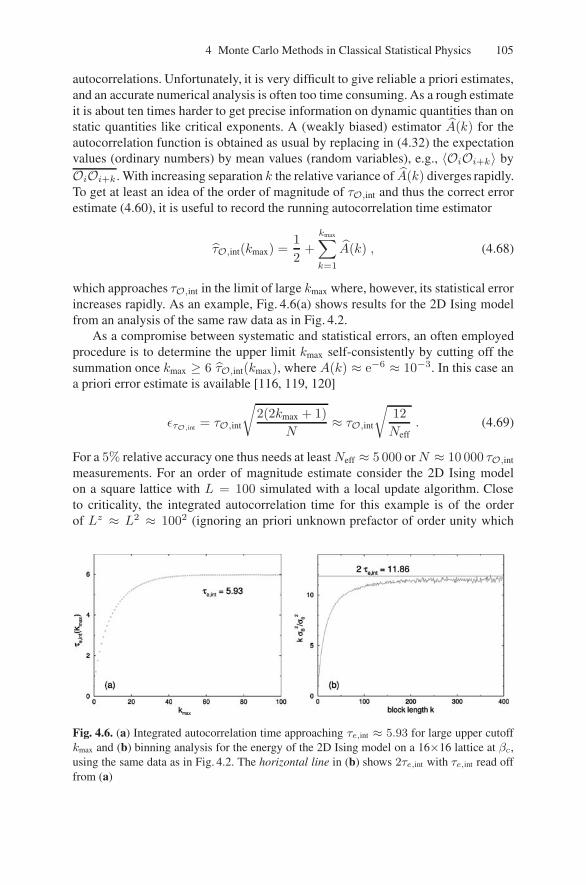
which approaches τO,int in the limit of large kmax where, however, its statistical errorincreases rapidly. As an example, Fig. 4.6(a) shows results for the 2D Ising modelfrom an analysis of the same raw data as in Fig. 4.2.

As a compromise between systematic and statistical errors, an often employedprocedure is to determine the upper limit kmax self-consistently by cutting off thesummation once kmax ≥ 6 τO,int(kmax), where A(k) ≈ e−6 ≈ 10−3. In this case ana priori error estimate is available [116, 119, 120]

ετO,int = τO,int

√2(2kmax + 1)

N≈ τO,int

√12Neff

. (4.69)

For a 5% relative accuracy one thus needs at leastNeff ≈ 5 000 orN ≈ 10 000 τO,int

measurements. For an order of magnitude estimate consider the 2D Ising modelon a square lattice with L = 100 simulated with a local update algorithm. Closeto criticality, the integrated autocorrelation time for this example is of the orderof Lz ≈ L2 ≈ 1002 (ignoring an priori unknown prefactor of order unity which

Fig. 4.6. (a) Integrated autocorrelation time approaching τe,int ≈ 5.93 for large upper cutoffkmax and (b) binning analysis for the energy of the 2D Ising model on a 16×16 lattice at βc,using the same data as in Fig. 4.2. The horizontal line in (b) shows 2τe,int with τe,int read offfrom (a)

106 W. Janke

depends on the considered quantity), implying N ≈ 108. Since in each sweep L2

spins have to be updated and assuming that each spin update takes about 0.1μsec,we end up with a total time estimate of about 105 s ≈ 1 CPU-day to achieve thisaccuracy.

An alternative is to approximate the tail end of A(k) by a single exponential asin (4.33). Summing up the small k part exactly, one finds [121]

τO,int(kmax) = τO,int − c e−kmax/τO,exp , (4.70)

where c is a constant. The latter expression may be used for a numerical estimate ofboth the exponential and integrated autocorrelation times [121].

4.5.4 Binning Analysis

It should be clear by now that ignoring autocorrelation effects can lead to severeunderestimates of statistical errors. Applying the full machinery of autocorrelationanalysis discussed above, however, is often too cumbersome. On a day by day basisthe following binning analysis is much more convenient (though somewhat less ac-curate). By grouping the N original time-series data into NB non-overlapping binsor blocks of length k (such that6 N = NBk), one forms a new, shorter time seriesof block averages

O(B)j ≡ 1

k

k∑i=1

O(j−1)k+i (4.71)

with j = 1, . . . , NB , which by choosing the block length k � τ are almost uncor-related and can thus be analyzed by standard means. The mean value over all blockaverages obviously satisfies O(B) = O and their variance can be computed accord-ing to the standard (unbiased) estimator, leading to the squared statistical error ofthe mean value

ε2O ≡ σ2O = σ2

B/NB =1

NB(NB − 1)

NB∑j=1

(O(B)j −O(B))2 . (4.72)

By comparing with (4.60) we see that σ2B/NB = 2τO,intσ

2Oi/N . Recalling the defi-

nition of the block length k = N/NB , this shows that one may also use

2τO,int = kσ2B/σ

2Oi

(4.73)

for the estimation of τO,int. This is demonstrated in Fig. 4.6(b). Estimates of τO,int

obtained in this way are often referred to as blocking τ or binning τ .A simple toy model (bivariate time series), where the behavior of the blocking

τ and also of τO,int(kmax) for finite k resp. kmax can be worked out exactly, is dis-cussed in [58]. These analytic formulas are very useful for validating the computerimplementations.

6 Here we assume that N was chosen cleverly. Otherwise one has to discard some of thedata and redefine N .


4.5.5 Jackknife Analysis

Even if the data are completely uncorrelated in time, one still has to handle theproblem of error estimation for quantities that are not directly measured in the sim-ulation but are computed as a non-linear combination of basic observables. Thisproblem can either be solved by error propagation or by using the Jackknife method[122, 123], where instead of considering rather small blocks of length k and theirfluctuations as in the binning method, one forms NB large Jackknife blocks O(J)

j

containing all data but the jth block of the previous binning method,

O(J)j =

NO − kO(B)j

N − k (4.74)

with j = 1, . . . , NB , cf. the schematic sketch in Fig. 4.7.Each of the Jackknife blocks thus consists of N − k data, i.e., it contains almost

as many data as the original time series. When non-linear combinations of basicvariables are estimated, the bias is hence comparable to that of the total data set(typically 1/(N − k) compared to 1/N ). The NB Jackknife blocks are, of course,trivially correlated because one and the same original data enter inNB − 1 differentJackknife blocks. This trivial correlation caused by re-using the original data overand over again has nothing to do with temporal correlations. As a consequence,the Jacknife block variance σ2

J will be much smaller than the variance estimated inthe binning method. Because of the trivial nature of the correlations, however, thisreduction can be corrected by multiplying σ2

J with a factor (NB − 1)2, leading to

ε2O ≡ σ2O =

NB − 1NB

NB∑j=1

(O(J)j −O(J))2 . (4.75)

To summarize this section, any realization of a Markov chain Monte Carlo up-date algorithm is characterized by autocorrelation times which enter directly into thestatistical errors of Monte Carlo estimates. Since temporal correlations always in-crease the statistical errors, it is thus a very important issue to develop Monte Carlo

O(J)NB

O(J)3

O(J)2

O(J)1

O

NB

3

2

1

Fig. 4.7. Schematic sketch of the organization of Jackknife blocks. The grey part of theN data points is used for calculating the total and the Jackknife block averages. The whiteblocks enter into the more conventional binning analysis using non-overlapping blocks

108 W. Janke

update algorithms that keep autocorrelation times as small as possible. This is thereason why cluster and other non-local algorithms are so important.

4.6 Reweighting Techniques

The physics underlying reweighting techniques [124, 125] is extremely simple andthe basic idea has been known since long (see the list of references in [125]), buttheir power in practice has been realized only relatively late in 1988. The impor-tant observation by Ferrenberg and Swendsen [124, 125] was that the best perfor-mance is achieved near criticality where histograms are usually broad. In this sensereweighting techniques are complementary to improved estimators, which usuallyperform best off criticality.

4.6.1 Single-Histogram Technique

The single-histogram reweighting technique [124] is based on the following verysimple observation. If we denote the number of states (spin configurations) thathave the same energy E by Ω(E), the partition function at the simulation pointβ0 = 1/kBT0 can always be written as7

Z(β0) =∑{s}

e−β0H({s}) =∑E

Ω(E)e−β0E ∝∑E

Pβ0(E) , (4.76)

where we have introduced the unnormalized energy histogram (density)

Pβ0(E) ∝ Ω(E)e−β0E . (4.77)

If we would normalize Pβ0(E) to unit area, the r.h.s. would have to be divided by∑E Pβ0(E) = Z(β0), but the normalization will be unimportant in what follows.

Let us assume we have performed a Monte Carlo simulation at inverse temperatureβ0 and thus know Pβ0(E). It is then easy to see that

Pβ(E) ∝ Ω(E)e−βE = Ω(E)e−β0Ee−(β−β0)E ∝ Pβ0(E)e−(β−β0)E , (4.78)

i.e., the histogram at any point β can be derived, in principle, by reweighting thesimulated histogram at β0 with the exponential factor exp[−(β−β0)E]. Notice thatin reweighted expectation values

〈f(E)〉(β) =∑

E f(E)Pβ(E)∑E Pβ(E)

, (4.79)

the normalization of Pβ(E) indeed cancels. This gives, for instance, the energy〈e〉(β) = 〈E〉(β)/V and the specific heat C(β) = β2V [〈e2〉(β) − 〈e〉(β)2], in


principle, as a continuous function of β from a single Monte Carlo simulation at β0,where V = LD is the system size.

As an example of this reweighting procedure, using actual Swendsen-Wangcluster simulation data (with 5 000 sweeps for equilibration and 50 000 sweeps formeasurements) of the 2D Ising model at β0 = βc = ln(1 +

√2)/2 = 0.440 686 . . .

on a 16×16 lattice with periodic boundary conditions, the specific heat C(β) isshown in Fig. 4.8(a) and compared with the curve obtained from the exact Kauf-man solution [12, 13] for finite Lx × Ly lattices. This clearly demonstrates that, inpractice, the β-range over which reweighting can be trusted is limited. The reasonfor this limitation are unavoidable statistical errors in the numerical determinationof Pβ0 using a Monte Carlo simulation. In the tails of the histograms the relativestatistical errors are largest, and the tails are exactly the regions that contribute mostwhen multiplying Pβ0(E) with the exponential reweighting factor to obtain Pβ(E)for β-values far off the simulation point β0. This is illustrated in Fig. 4.8(b) wherethe simulated histogram at β0 = βc is shown together with the reweighted his-tograms at β = 0.375 ≈ β0 − 0.065 and β = 0.475 ≈ β0 + 0.035, respectively.For the 2D Ising model the quality of the reweighted histograms can be judged bycomparing with the curves obtained from Beale’s [112] exact expression for Ω(E).

4.6.1.1 Reweighting Range

As a rule of thumb, the range over which reweighting should produce accurateresults can be estimated by requiring that the peak location of the reweighted his-

0.3β

0

1

2

spec

ific

heat

2D Ising

162

(a)

0.60.50.4 0.5−E/V

0

10

coun

ts

β = 0.375 β = 0.475

β0 = βc

(b)

1.0 1.5 2.0

Fig. 4.8. (a) The specific heat of the 2D Ising model on a 16×16 square lattice computedby reweighting from a single Monte Carlo simulation at β0 = βc, marked by the filled datasymbol. The continuous line shows for comparison the exact solution of Kaufman [12, 13].(b) The corresponding energy histogram at β0, and reweighted to β = 0.375 and β = 0.475.The dashed lines show for comparison the exact histograms obtained from Beale’s expression[112]

7 For simplicity we consider here only models with discrete energies. If the energy variescontinuously, sums have to be replaced by integrals, etc. Also lattice size dependences aresuppressed to keep the notation short.

110 W. Janke

togram should not exceed the energy value at which the input histogram had de-creased to about one half or one third of its maximum value. In most applicationsthis range is wide enough to locate from a single simulation, e.g., the specific-heatmaximum by employing a standard maximization subroutine to the continuous func-tion C(β). This is by far more convenient, accurate and faster than the traditionalway of performing many simulations close to the peak of C(β) and trying to deter-mine the maximum by spline or least-squares fits.

For an analytical estimate of the reweighting range we now require that the peakof the reweighted histogram is within the width 〈e〉(T0) ± Δe(T0) of the inputhistogram (where a Gaussian histogram would have decreased to exp(−1/2) ≈0.61 of its the maximum value)

|〈e〉(T )− 〈e〉(T0)| ≤ Δe(T0) , (4.80)

where we have made use of the fact that for a not too asymmetric histogram Pβ0(E)the maximum location approximately coincides with 〈e〉(T0). Recalling that the halfwidth Δe of a histogram is related to the specific heat via (Δe)2 ≡ 〈(e − 〈e〉)2〉 =〈e2〉 − 〈e〉2 = C(β0)/β2

0V and using the Taylor expansion 〈e〉(T ) = 〈e〉(T0) +C(T0)(T − T0) + . . ., this can be written as C(T0)|T − T0| ≤ T0

√C(T0)/V or

|T − T0|T0

≤ 1√V C(T0)

. (4.81)

SinceC(T0) is known from the input histogram this is quite a general estimate of thereweighting range. For the example in Fig. 4.8 with V =16×16, β0 = βc ≈ 0.44and C(T0) ≈ 1.5, this estimate yields |β − β0|/β0 ≈ |T − T0|/T0 ≤ 0.04, i.e.,|β− β0| ≤ 0.02 or 0.42 ≤ β ≤ 0.46. By comparison with the exact solution we seethat this is indeed a fairly conservative estimate of the reliable reweighting range.

If we only want to know the scaling behavior with system size V = LD, we cango one step further by considering three generic cases:

(i) Off-criticality, where C(T0) ≈ const, such that

|T − T0|T0

∝ V −1/2 = L−D/2 . (4.82)

(ii) Criticality, where C(T0) � a1 + a2Lα/ν , with a1 and a2 being constants, and

α and ν denoting the standard critical exponents of the specific heat and cor-relation length, respectively. For α > 0, the leading scaling behavior becomes|T − T0|/T0 ∝ L−D/2L−α/2ν . Assuming hyperscaling (α = 2 − Dν) to bevalid, this simplifies to

|T − T0|T0

∝ L−1/ν , (4.83)

i.e., the typical scaling behavior of pseudo-transition temperatures in the finite-size scaling regime of a second-order phase transition [126]. For α < 0, C(T0)approaches asymptotically a constant and the leading scaling behavior of thereweighting range is as in the off-critical case.


(iii) First-order transitions, where C(T0) ∝ V . This yields

|T − T0|T0

∝ V −1 = L−D , (4.84)

which is again the typical finite-size scaling behavior of pseudo-transition tem-peratures close to a first-order phase transition [47].

4.6.1.2 Reweighting of Non-Conjugate Observables

If we also want to reweight other quantities such as the magnetization 〈m〉 wehave to go one step further. The conceptually simplest way would be to store two-dimensional histogramsPβ0(E,M) whereM = V m is the total magnetization. Wecould then proceed in close analogy to the preceding case, and even reweighting tonon-zero magnetic field h would be possible, which enters via the Boltzmann fac-tor exp(βh

∑i si) = exp(βhM). However, the storage requirements may be quite

high (of the order of V 2), and it is often preferable to proceed in the following way.For any function g(M), e.g., g(M) = Mk, we can write

〈g(M)〉 =∑{s}

g(M({s}))e−β0H/Z(β0)

=∑E,M

Ω(E,M)g(M)e−β0E/Z(β0)

=∑E

∑M Ω(E,M)g(M)∑

M Ω(E,M)

∑M

Ω(E,M)e−β0E/Z(β0) . (4.85)

Recalling that∑

M Ω(E,M)e−β0E/Z(β0) = Ω(E)e−β0E/Z(β0) = Pβ0(E) anddefining the microcanonical expectation value of g(M) at fixed energy E (some-times denoted as a list)

〈〈g(M)〉〉(E) ≡∑

M Ω(E,M)g(M)∑M Ω(E,M)

, (4.86)

we arrive at〈g(M)〉 =

∑E

〈〈g(M)〉〉(E)Pβ0 (E) . (4.87)

Identifying 〈〈g(M)〉〉(E) with f(E) in (4.79), the actual reweighting procedure isprecisely as before. An example for computing 〈〈|M |〉〉(E) and 〈〈M2〉〉(E) usingthe data of Fig. 4.8 is shown in Fig. 4.9. Mixed quantities, e.g. 〈EkM l〉, can betreated similarly. One caveat of this method is that one has to decide beforehandwhich lists 〈〈g(M)〉〉(E) one wants to store during the simulation, e.g., which pow-ers k in 〈〈Mk〉〉(E) are relevant.

An alternative and more flexible method is based on time series. Suppose wehave performed a Monte Carlo simulation at β0 and stored the time series of N

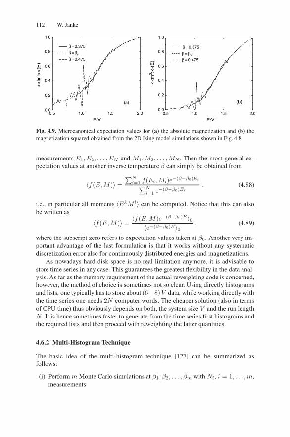
112 W. Janke

0.5 1.0 1.5 2.0

−E/V

0.0

0.2

0.4

0.6

0.8

1.0<

<|m

|>>

(E)

β = 0.375

β = βc

β = 0.475

(a)

0.5 1.0 1.5 2.0

−E/V

0.0

0.2

0.4

0.6

0.8

1.0

<<

m2 >

>(E

)

β = 0.375

β = βc

β = 0.475

(b)

Fig. 4.9. Microcanonical expectation values for (a) the absolute magnetization and (b) themagnetization squared obtained from the 2D Ising model simulations shown in Fig. 4.8

measurements E1, E2, . . . , EN and M1,M2, . . . ,MN . Then the most general ex-pectation values at another inverse temperature β can simply be obtained from

〈f(E,M)〉 =∑Ni=1 f(Ei,Mi)e−(β−β0)Ei∑N

i=1 e−(β−β0)Ei

, (4.88)

i.e., in particular all moments 〈EkM l〉 can be computed. Notice that this can alsobe written as

〈f(E,M)〉 = 〈f(E,M)e−(β−β0)E〉0〈e−(β−β0)E〉0 , (4.89)

where the subscript zero refers to expectation values taken at β0. Another very im-portant advantage of the last formulation is that it works without any systematicdiscretization error also for continuously distributed energies and magnetizations.

As nowadays hard-disk space is no real limitation anymore, it is advisable tostore time series in any case. This guarantees the greatest flexibility in the data anal-ysis. As far as the memory requirement of the actual reweighting code is concerned,however, the method of choice is sometimes not so clear. Using directly histogramsand lists, one typically has to store about (6−8)V data, while working directly withthe time series one needs 2N computer words. The cheaper solution (also in termsof CPU time) thus obviously depends on both, the system size V and the run lengthN . It is hence sometimes faster to generate from the time series first histograms andthe required lists and then proceed with reweighting the latter quantities.

4.6.2 Multi-Histogram Technique

The basic idea of the multi-histogram technique [127] can be summarized asfollows:

(i) Perform m Monte Carlo simulations at β1, β2, . . . , βm with Ni, i = 1, . . . ,m,measurements.


(ii) Reweight all runs to a common reference point β0.(iii) Combine at β0 all information by computing error weighted averages.(iv) Reweight the combined histogram to any other β.

Here we shall assume that the histograms Pβi(E) are naturally normalized∑E Pβi(E) = Ni, such that the statistical errors for each of the histograms Pβi(E)

are approximately given by√Pβi(E). By choosing as reference point β0 = 0 and

working out the error weighted combined histogram one ends up with

Ω(E) =∑mi=1 Pβi(E)∑m

i=1NiZ−1i e−βiE

, (4.90)

where the unknown partition function values Zi ≡ Z(βi) are determined self-consistently from

Zi =∑E

Ω(E)e−βiE =∑E

e−βiE

∑mk=1 Pβk

(E)∑mk=1NkZ

−1k e−βkE

, (4.91)

up to an unimportant overall constant. A good starting point for the recursion isto fix, say, Z1 = 1 and use single histogram reweighting to get an estimate ofZ2/Z1 = exp[−(F2 − F1)], where Fi = βiF (βi). Once Z2 is determined, thesame procedure can be applied to estimate Z3 and so on. In the limit of infinitestatistics, this would already yield the solution of (4.91). In realistic simulationsthe statistics is of course limited and the (very few) remaining recursions averagethis uncertainty to get a self-consistent set of Zi. In order to work in practice, thehistograms at neighboring β-values must have sufficient overlap, i.e., the spacingsof the simulation points must be chosen according to the estimates (4.82)–(4.84).

Multiple-histogram reweighting has been widely applied in many different ap-plications. Some problems of this method are that autocorrelations cannot properlybe taken into account when computing the error weighted average (which is still cor-rect but no longer optimized), the procedure for computing mixed quantities suchas 〈EkM l〉 is difficult to justify (even though it does work as an ad hoc prescriptionquite well), and the statistical error analysis becomes quite cumbersome.

As an alternative one may compute by reweighting from each of the m simula-tions all quantities of interest as a function of β, including their statistical error barswhich now also should take care of autocorrelations as discussed in Sect. 4.5.2.3.In this way one obtains, at each β-value, m estimates, e.g. e1(β) ± Δe1, e2(β) ±Δe2, . . . , em(β)±Δem, which may be optimally combined according to their errorbars to give e(β)±Δe. If the relative errorΔe/e(β) is minimized, this leads to [87]

e(β) =

(e1(β)(Δe1)

2 +e2(β)

(Δe2)2 + . . .+

em(β)(Δem)2

)(Δe)2 , (4.92)

with1

(Δe)2=

1

(Δe1)2 +

1

(Δe2)2 + . . .+

1

(Δem)2. (4.93)

Notice that in this way the average for each quantity can be individually optimized.

114 W. Janke

4.7 Finite-Size Scaling Analysis

Equipped with the various technical tools discussed above, the purpose of this sec-tion is to outline a typical FSS analysis of Monte Carlo simulations of second-orderphase transitions. The described procedure is generally applicable but to keep thenotation short, all formulas are formulated for Ising like systems. For instance forO(n) symmetric models, m should be replaced by m etc. The main results of suchstudies are usually estimates of the critical temperature and the critical exponentscharacterizing the universality class of the transition.

4.7.1 General Framework

To facilitate most flexibility in the analysis, it is advisable to store during data pro-duction the time series of measurements. Standard quantities are the energy andmagnetization, but depending on the model at hand it may be useful to record alsoother observables. In this way the full dynamical information can be extracted stillafter the actual simulation runs and error estimation can be easily performed. Forexample it is no problem to experiment with the size and number of Jackknife bins.Since a reasonable choice depends on the a priori unknown autocorrelation time,it is quite cumbersome to do a reliable error analysis on the flight during the sim-ulation. Furthermore, basing data reweighting on time-series data is more efficientsince histograms, if needed or more convenient, can still be produced from this databut working in the reverse direction is obviously impossible.

For some models it is sufficient to perform for each lattice size a single longrun at some coupling β0 close to the critical point βc. This is, however, not alwaysthe case and also depends on the observables of interest. In this more general case,one may use several simulation points βi and combine the results by the multi-histogram reweighting method or may apply a very recently developed finite-sizeadapted generalized ensemble method [128]. In both situations, one can computefrom the time series of the energies e = E/V (ifE happens to be integer valued, thisshould be stored of course) by reweighting the internal energy 〈e〉(β), the specificheat C(β) = β2 V

(〈e2〉 − 〈e〉2), and for instance also the energetic fourth-orderparameter

V (β) = 1− 〈e4〉3〈e2〉2 (4.94)

as a function of temperature. Similarly, from measurements of the magnetiza-tion m = M/V one can derive the temperature variation of the mean mag-netization8 m(β) = 〈|m|〉, the susceptibility χ(β) = β V

(〈m2〉 − 〈|m|〉2) (orχ′(β) = βV 〈m2〉 for β ≤ βc), the magnetic cumulants (Binder parameters)

8 Notice that here and in the following formulas, |m| is used instead of m as wouldfollow from the formal definition (4.5) of the zero-field magnetization m(β) =1/(V β) limh→0 ∂ lnZ(β, h)/∂h. The reason is that for a symmetric model on finite lat-tices one obtains 〈m〉(β) = 0 for all temperatures due to symmetry. Only in the properinfinite-volume limit, that is limh→0 limV →∞, spontaneous symmetry breaking can occurbelow Tc. In a simulation on finite lattices, this is reflected by a symmetric double-peak


U2(β) = 1− 〈m2〉3〈|m|〉2 ,

U4(β) = 1− 〈m4〉3〈m2〉2 , (4.95)

and their slopes

dU2(β)dβ

=V

3〈|m|〉2[⟨m2

⟩ 〈e〉 − 2

⟨m2

⟩ 〈|m|e〉〈|m|〉 + 〈m2e〉

]

= V (1 − U2)[〈e〉 − 2

〈|m|e〉〈|m|〉 +

〈m2e〉〈m2〉

],

dU4(β)dβ

= V (1 − U4)[〈e〉 − 2

〈m2e〉〈m2〉 +

〈m4e〉〈m4〉

]. (4.96)

Further quantities with a useful FSS behavior are the derivatives of the magnetiza-tion,

d〈|m|〉dβ

= V (〈|m|e〉 − 〈|m|〉〈e〉) ,d ln〈|m|〉

dβ= V

( 〈|m|e〉〈|m|〉 − 〈e〉

),

d ln〈m2〉dβ

= V

( 〈m2e〉〈m2〉 − 〈e〉

). (4.97)

These latter five quantities are good examples for expectation values containingboth, powers of e and m.

In the infinite-volume limit most of these quantities exhibit singularities at thetransition point. As already discussed in Sect. 4.2, in finite systems the singularitiesare smeared out and the standard observables scale in the critical region according to

C = Creg + Lα/νfC(x)[1 + . . .] , (4.98)

〈|m|〉 = L−β/νfm(x)[1 + . . .] , (4.99)

χ = Lγ/νfχ(x)[1 + . . .] , (4.100)

where Creg is a regular background term, α, ν, β (in the exponent of L) and γ arethe usual critical exponents, and fi(x) are FSS functions with

structure of the magnetization distribution (provided the runs are long enough). By aver-aging m one thus gets zero by symmetry, while the peak locations ±m0(L) are close tothe spontaneous magnetization and the average of |m| is a good estimator. Things becomemore involved for slightly asymmetric models, where this recipe would produce a sys-tematic error and thus cannot be employed. For strongly asymmetric models, on the otherhand, one peak clearly dominates and the average of m can usually be measured withouttoo many problems.

116 W. Janke

x = (β − βc)L1/ν (4.101)

being the scaling variable (do not confuse the unfortunate double-meaning of β –here β = 1/kBT ). The brackets [1+. . .] indicate corrections-to-scaling terms whichbecome unimportant for sufficiently large system sizes L.

A particular role play the magnetic cumulants or Binder parameters U2 and U4

which scale according to

U2p = fU2p(x)[1 + . . .] , (4.102)

i.e., for constant scaling variable x, they take approximately the same value forall lattice sizes, in particular U∗

2p ≡ fU2p(0) at βc. Their curves as function oftemperature for differentL hence cross around (βc, U∗

2p) (with slopes∝ L1/ν), apartfrom corrections-to-scaling collected in [1 + . . .] which explain small systematicdeviations. From a determination of this crossing point, one thus obtains a basicallyunbiased estimate of βc, the critical exponent ν, and U∗

2p. Note that in contrast to thetruly universal critical exponents, U∗

2p is only weakly universal. By this one meansthat the infinite-volume limit of such quantities does depend in particular on theboundary conditions and geometrical shape of the considered lattice, e.g., on theaspect ratio r = Ly/Lx [129, 130, 131, 132, 133, 134, 135, 136].

Differentiating U2p with respect to β, one picks up an extra power of L from thescaling function, dU2p/dβ = (dx/dβ)f ′

U2p= L1/νf ′

U2p. This leads to

dU2p

dβ= L1/νf ′

U2p(x)[1 + . . .] , (4.103)

and similarly for the magnetization derivatives

d〈|m|〉dβ

= L(1−β)/νf ′m(x)[1 + . . .] , (4.104)

d ln〈|m|p〉dβ

= L1/νfdmp(x)[1 + . . .] . (4.105)

By applying standard reweighting techniques to the time-series data one firstdetermines the temperature dependence of C(β), χ(β), . . . , in the neighborhoodof the simulation point β0 ≈ βc (a reasonably good guess of β0 can usually beobtained quite easily from a few short test runs). It should be stressed that in aserious study, by estimating the valid reweighting range, one should at any ratemake sure that no systematic errors crept in by this procedure (which may be eas-ily overlooked if one works too mechanically). Once the temperature dependenceis known, one can determine the maxima, e.g., Cmax(βmaxC ) ≡ maxβ C(β), byapplying standard extremization routines: When reweighting is implemented as asubroutine, for instance C(β) can be handled as a normal function with a con-tinuously varying argument β, i.e., no interpolation or discretization error is in-volved when iterating towards the maximum. The locations of the maxima of C,χ, dU2/dβ, dU4/dβ, d〈|m|〉/dβ, d ln〈|m|〉/dβ, and d ln〈m2〉/dβ provide us with


seven sequences of pseudo-transition points βmaxi(L) which all should scale ac-

cording to βmaxi(L) = βc + aiL

−1/ν + . . .. In other words, the scaling variablex = (βmaxi(L) − βc)L1/ν = ai + . . . should be constant, if we neglect the smallhigher-order corrections indicated by . . ..

Notice that while the precise estimates of ai do depend on the value of ν, thequalitative conclusion that x ≈ const for each of the βmaxi

(L) sequences does notrequire any a priori knowledge of ν or βc. Using this information one thus hasseveral possibilities to extract unbiased estimates of the critical exponents ν, α/ν,β/ν, and γ/ν from least-squares fits assuming the FSS behaviors (4.98)–(4.105).

4.7.2 A Practical Recipe

The typical procedure of an FSS analysis then proceeds as follows:

(i) Estimate the critical exponent ν by least-square fits to the scaling behavior(4.103) and (4.105). For this one may consider directly the maxima of dU2p/dβand d ln〈|m|p〉/dβ, p = 1, 2, or work with any other FSS sequence βmaxi

(L).

Remarks: Considering only the asymptotic behavior, e.g., d ln〈|m|〉/dβ =aL1/ν , and taking the logarithm, ln(d ln〈|m|〉/dβ) = c+(1/ν) ln(L), one endsup with a linear two-parameter fit yielding estimates for the constant c = ln(a)and the exponent 1/ν. For small lattice sizes the asymptotic ansatz is, of course,not justified. Taking into account the (effective) correction term [1 + bL−w]would result in a non-linear four-parameter fit for a, b, 1/ν and w. Even if wewould fix w to some theoretically expected value (as is sometimes done), wewould be still left with a non-linear fit which is usually much harder to controlthan a linear fit (where only a set of linear equations with a unique solutionhas to be solved, whereas a non-linear fit involves a numerical minimizationof the χ2-function, possessing possibly several local minima). The alternativemethod is to use the linear fit ansatz and to discard successively more and moresmall lattice sizes until the χ2 per degree of freedom or the goodness-of-fit Q[113] has reached an acceptable value and does not show any further trend. Ofcourse, all this relies heavily on correct estimates of the statistical error bars onthe original data for d ln〈|m|〉/dβ.

Furthermore, when combining the various fit results for ν to a final value,some care is necessary with the final statistical error estimate on ν, since thevarious fits for determining ν are of course correlated (since they use the datafrom one and the same simulation).

(ii) Once ν is estimated one can use the scaling formβmaxi(L) = βc+aiL−1/ν+. . .

to extract βc and ai. As a useful check, one should repeat these fits at the errormargins of ν, but usually this dependence turns out to be very weak.

Remark: Regarding the βc fit alone, the uncertainty in the proper value of νlooks like a kind of systematic error or bias, whose origin, however, is also ofstatistical nature occurring in the first step.

118 W. Janke

(iii) As a useful cross-check one can determine βc also from the Binder parametercrossings. For a first rough estimate, this is a very convenient and fast method.

Remarks: As a rule of thumb, an accuracy of about 3–4 digits for βc can beobtained with this method without any elaborate infinite-volume extrapolations– the crossing points lie usually much closer to βc than the various maximalocations. For high precision, however, it is quite cumbersome to control thenecessary extrapolations and often more accurate estimates can be obtainedby considering the scaling of the maxima locations. Also, error estimates ofcrossing points involve the data for two different lattice sizes which tends to bequite unhandy.

(iv) Next, similarly to ν, the ratios of critical exponents α/ν, β/ν, and γ/ν can beobtained from fits to (4.98)–(4.100), and (4.104). Again the maxima of thesequantities or any of the FSS sequences βmaxi

can be used. What concerns thefitting procedure the same remarks apply as for ν.

Remarks: The specific heat C usually plays a special role in that the expo-nent α is difficult to determine. The reason is that α is usually relatively small(3D Ising model: α ≈ 0.1), may be zero (logarithmic divergence as in the 2DIsing model) or even negative (as for instance in the 3D XY and Heisenbergmodels). In all these cases, the constant background contributionCreg in (4.98)becomes important, which enforces a non-linear three-parameter fit with thejust described problems. Also for the susceptibility χ, a regular backgroundterm cannot be excluded, but it is usually much less important since γ � α.Therefore, in (4.99), (4.100), and (4.104), similar to the fits for ν, one may takethe logarithm and work with much more stable linear fits.

(v) As a final step one may re-check the FSS behavior of C, χ, dU2/dβ, . . . at thenumerically determined estimate of βc. These fits should be repeated also atβc ± Δβc in order to estimate by how much the uncertainty in βc propagatesinto the thus determined exponent estimates.

Remark: In (the pretty rare) cases where βc is known exactly (e.g., through self-duality), this latter option is by far the most accurate one. This is the reason,why for such models numerically estimated critical exponents are usually alsomuch more precise.

4.7.3 Finite-Size Scaling at Work – An Example

The purpose of this subsection is to illustrate the above outlined recipe with ac-tual data from recent simulations of a 2D Ising model with next-nearest neighborinteractions [137]. The Hamiltonian has the form

H = −J∑〈i,j〉

σiσj − Jd

∑(k,l)

σkσl , (4.106)

where the spins can take the values σi = ±1, J denotes the nearest-neighbor (nn)coupling and Jd is the next-nearest-neighbor (nnn) coupling along the two diagonals


of a square lattice. The corresponding pairs of spins are denoted by the brack-ets 〈i, j〉 and (k, l), respectively. In [137] we restricted ourselves to that regionof the phase diagram where the ground states show ferromagnetic order (J ≥ 0,Jd ≥ −J/2), and always assumed periodic boundary conditions. Absorbing the nncoupling J into the inverse temperature β (i.e., formally putting J = 1), the remain-ing second parameter is the coupling-constant ratio α = Jd/J . In the following wewill concentrate on the case α = 0.5 [138]. The linear size of the lattices varies fromL = 10, 20, 40, . . . up to 640. All simulations are performed with the single-clusteralgorithm which is straightforward to adapt to nnn interactions by setting bonds alsoalong the diagonals. Similarly to the standard nn model, the integrated autocorrela-tion time close to criticality is found for α = 1 [137] to scale only weakly withlattice size: τe,int ∝ Lz with z = 0.134(3).

Another example following closely the lines sketched above is provided by aMonte Carlo study of the 3D Ising model, albeit not on a regular but on Poissonnianrandom lattices of Voronoi-Delaunay type [139]. The random lattices are treated asquenched disorder in the local coordination numbers and hence necessitate an ad-ditional average over many realizations (in the study described in [139], for eachlattice size 96 independent realizations were used). This introduces in all FSS for-mulas additional disorder averages which complicate some aspects of the analysis.The general concept of FSS analysis, however, does not depend on this special fea-ture and it may be worthwhile to consult [139] for a supplementary example.

4.7.3.1 Critical Exponent ν

Having recorded the times series of the energy and magnetization, all quantities ofthe preceding paragraph can be computed in the FSS region. The scaling behaviorof the maxima of d ln〈|m|p〉/dβ and dU2p/dβ for p = 1 and p = 2 is shown in

(dU2/dβ)max

(dU4/dβ)max

(d ln⏐m⏐/dβ)max

(d ln m2/dβ)max

ln L

lnO m

ax

765432

9

8

7

6

5

4

3

2

1

0

Fig. 4.10. FSS of the maxima of d ln〈|m|p〉/dβ and dU2p/dβ for p = 1 and p = 2 of the2D nnn Ising model (4.106) with α = Jd/J = 0.5 and fits to extract 1/ν

120 W. Janke

Table 4.3. Fit results for the correlation length critical exponent ν of the 2D nnn Ising modelwith α = Jd/J = 0.5, and the weighted average of the four estimates. Also listed are the χ2

per degree of freedom, χ2/d.o.f., and the goodness-of-fit parameter Q [113]

d ln〈|m|〉/dβ d ln〈m2〉/dβ dU2/dβ dU4/dβ weighted av.

ν 1.0031(17) 1.0034(21) 1.0027(24) 1.0025(44) 1.0031(11)χ2/d.o.f 0.98 0.60 2.02 0.49Q 0.37 0.55 0.13 0.61

the log-log plot of Fig. 4.10. From the parameters of the four linear fits over thedata points with Lmin > 40 collected in Table 4.3, we obtain a weighted average ofν = 1.003 1± 0.001 1.

As the more detailed analysis in [139] clearly shows, considering all 4×7 =28 possible FSS sequences (the four observables shown in Fig. 4.10 evaluated atthe seven different βmaxi

sequences) does not significantly improve the precisionof the final estimate. The reason are the quite strong correlations between most ofthese 28 estimates. In a really large-scale simulation such a more detailed analysismay still be valuable, however, since it potentially helps to detect systematic trendswhich otherwise may remain unnoticed. Also here the weighted average is clearlydominated by the result from the d ln〈|m|〉/dβ fit, and correlations between the firstand second pair of estimates are obvious. Therefore, to account for these correlationsat least heuristically, we usually quote in our investigations the weighted average,but take the smallest contributing error estimate (here thus from the d ln〈|m|〉/dβfit). This recipe then gives from Table 4.3 the final result

ν = 1.003 1± 0.001 7 , (4.107)

in good agreement with the 2D Ising universality class (cf. Table 4.1).

4.7.3.2 Critical Coupling βcβcβc

Fixing the critical exponent ν at the numerically determined estimate (or in thepresent context at the exactly known value ν = 1), it is now straightforward toobtain estimates of the critical coupling βc from linear least-squares fits to

βmaxi = βc + aiL−1/ν , (4.108)

where βmaxiare the pseudo-transition points discussed earlier. Depending on the

quantity considered, here we found a significant improvement of the fit quality if thesmallest lattice sizes were excluded. This is illustrated in Table 4.4, where detailedresults for various fit ranges are compiled.

As final result we quote the weighted average of the five estimates and again thesmallest contributing error bar,

βc = 0.262 817 4± 0.000 0017 . (4.109)


Table 4.4. FSS fits of the pseudo-transition points βmax = βc + aL−1/ν of the nnn model(4.106) with α = 0.5 for varying fit ranges, assuming ν = 1. Here n is the number of datapoints, Lmin denotes the smallest lattice size considered, and Q is the standard goodness-of-fitparameter. The selected fit ranges used for the final average are high-lighted in boldface. Thelast line labeled HTS gives a high-temperature series estimate [140] for comparison

observables n Lmin βc Q

βCmax 7 10 0.262 699(13) 0.00

6 20 0.262 766(15) 0.035 40 0.262 799(18) 0.884 80 0.262 807(22) 0.89

β|m|inf 7 10 0.262 8706(36) 0.00

6 20 0.262 8398(40) 0.005 40 0.262 8272(47) 0.164 80 0.262 8212(58) 0.38

βχmax 7 10 0.262 8253(12) 0.00

6 20 0.262 8195(13) 0.005 40 0.262 8178(14) 0.094 80 0.262 8153(17) 0.66

βln |m|inf 7 10 0.262 8437(62) 0.00

6 20 0.262 8243(68) 0.245 40 0.262 8183(77) 0.424 80 0.262 8099(97) 0.70

βln m2

inf 7 10 0.262 8684(94) 0.006 20 0.262 837(11) 0.435 40 0.262 837(13) 0.574 80 0.262 818(17) 0.55

average 0.262 8204(144)weighted average 0.262 8174(16)final 0.262 8174(17)

HTS (Oitmaa [140]) 0.262 808

The corrections to the asymptotic FSS behavior can be also visually inspectedin Fig. 4.11, where the Monte Carlo data and fits are compared. One immediatelynotices a systematic trend that the L = 10 data deviate from the linear behavior.For larger L, however, the deviations are already so small that only a quantitativejudgement in terms of the χ2 per degree of freedom or goodness-of-fit parameterQof the fits [113] can lead to a sensible conclusion.

4.7.3.3 Binder Parameters U2 and U4

Following our general recipe sketched above, the Binder parameter U4(L) is shownin Fig. 4.12 as a function of temperature. Even though the temperature range is much

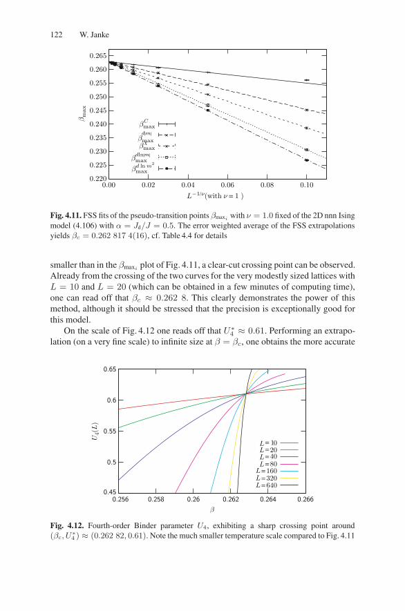
122 W. Janke

βmaxd ln m2

βmaxdln|m|

βmaxχ

βmax

d|m|

βmaxC

L−1/ν(with ν = 1 )

βm

ax

0.100.080.060.040.020.00

0.265

0.260

0.255

0.250

0.245

0.240

0.235

0.230

0.225

0.220

Fig. 4.11. FSS fits of the pseudo-transition points βmaxi with ν = 1.0 fixed of the 2D nnn Isingmodel (4.106) with α = Jd/J = 0.5. The error weighted average of the FSS extrapolationsyields βc = 0.262 817 4(16), cf. Table 4.4 for details

smaller than in the βmaxiplot of Fig. 4.11, a clear-cut crossing point can be observed.

Already from the crossing of the two curves for the very modestly sized lattices withL = 10 and L = 20 (which can be obtained in a few minutes of computing time),one can read off that βc ≈ 0.262 8. This clearly demonstrates the power of thismethod, although it should be stressed that the precision is exceptionally good forthis model.

On the scale of Fig. 4.12 one reads off that U∗4 ≈ 0.61. Performing an extrapo-

lation (on a very fine scale) to infinite size at β = βc, one obtains the more accurate

L= 640L= 320L= 160L 80L 40L 20L 10

β

U4(L

)

0.2660.2640.2620.260.2580.256

0.65

0.6

0.55

0.5

0.45

====

Fig. 4.12. Fourth-order Binder parameter U4, exhibiting a sharp crossing point around(βc, U

∗4 ) ≈ (0.262 82, 0.61). Note the much smaller temperature scale compared to Fig. 4.11


estimate of U∗4 = 0.610 8(1). This result for the 2D nnn Ising model with α = 0.5

is in perfect agreement with the very precisely known value for the standard squarelattice nn Ising model with periodic boundary conditions from extrapolating exacttransfer-matrix data for L ≤ 17 [129], U∗

4 = 0.610 690 1(5), and a numericalevaluation of an exact expression [130], U∗

4 = 0.610 692(2). This illustrates the ex-pected universality of U∗

4 (and also U∗2 ) for general isotropic interactions (e.g., also

for α = 1 one finds the same result within error bars [137]), as long as boundaryconditions, lattice shapes etc. are the same. As emphasized already in Sect. 4.7.1,the cumulants are, however, only weakly universal in the sense that they do dependsensitively on the anisotropy of interactions, boundary conditions and lattice shapes(aspect ratios) [131, 132, 133, 134, 135, 136].

4.7.3.4 Critical Exponent γγγ

The exponent ratio γ/ν can be obtained from fits to the FSS behavior (4.100) ofthe susceptibility. By monitoring the quality of the fits, using all data starting fromL = 10 is justified. The fits collected in Table 4.5 all have Q ≥ 0.15.

Still it is fairly obvious, that the two fits with Q < 0.2 have some problems.Discarding them in the averages, one obtains from the weighted average (and againquoting the smallest contributing error estimate to heuristically take into account thecorrelations among the individual fits)

Table 4.5. Fit results for the critical exponents γ/ν, β/ν, and (1−β)/ν. The fits for γ/ν and(1 − β)/ν take all lattices with L ≥ 10 into account while the fits for β/ν start at L = 20

at Kmax of γ/ν Q β/ν Q (1 − β)/ν Q

C 1.7574(28) 0.87 0.12856(38) 0.00 0.8889(13) 0.00

χ 1.7407(10) 0.16 0.12480(32) 0.45 0.8710(24) 0.93

dU4/dβ 1.7700(50) 0.40 0.12481(39) 0.51 0.9154(99) 0.38

dU2/dβ 1.7417(12) 0.42 0.12562(32) 0.02 0.8815(35) 0.39

d〈|m|〉/dβ 1.7356(11) 0.19 0.12191(33) 0.00 0.8760(15) 0.82

d ln〈|m|〉/dβ 1.7520(20) 0.62 0.12407(34) 0.02 0.8923(49) 0.57

d ln〈m2〉/dβ 1.7630(32) 0.76 0.12363(37) 0.01 0.9047(68) 0.81

average 1.7515(49) ≥ 0 0.12477(78) ≥ 0 0.8900(60) ≥ 0

weighted av. 1.7423(06) 0.12468(13) 0.8822(09)

final 1.7423(10) 0.12468(32) 0.8822(13)

average 1.7568(49) ≥ 0.2 0.12483(32) ≥ 0.02 0.8901(71) ≥ 0.3

weighted av. 1.7477(09) 0.12485(17) 0.8775(11)

final 1.7477(12) 0.12485(32) 0.8775(15)

exact 1.75 0.125 0.875

124 W. Janke

γ/ν = 1.747 7± 0.001 2 (4.110)

to be compared with the exact result 7/4 = 1.75. For the critical exponent η, theestimate (4.110) implies η = 2 − γ/ν = 0.252 3 ± 0.001 2, and, by insertingour value of ν = 1.003 1(17), one obtains γ = 1.753 1 ± 0.004 2. Here and inthe following we are quite conversative and always quote the maximal error, i.e.,max{(O1 + ε1)(O2 + ε2)−O1O2, O1O2 − (O1 − ε1)(O2 − ε2)}.

4.7.3.5 Critical Exponent β

The exponent ratio β/ν can be obtained either from the FSS behavior of 〈|m|〉or d〈|m|〉/dβ, (4.99) or (4.104). In the first case, Table 4.5 shows that most βmaxi

sequences yield poor Q values (≤ 0.1) even if the L = 10 lattice data is discarded.If one averages only the fits with Q ≥ 0.02, the final result is

β/ν = 0.124 85± 0.000 32 , (4.111)

and, by using our estimate (4.107) for ν, β = 0.125 23 ± 0.000 54, in very goodagreement with the exact result β/ν = β = 1/8 = 0.125 00 for the 2D Isinguniversality class. Assuming hyperscaling to be valid, the estimate (4.111) impliesγ/ν = D − 2β/ν = 1.750 30(64).

From the Q values in Table 4.5 one can conclude that the FSS of d〈|m|〉/dβ issomewhat better behaved, so that one can keep again all lattice sizes L ≥ 10 in thefits. By discarding only the fit for the βmaxC

sequence, which has an exceptionallysmall Q value, one arrives at

(1 − β)/ν = 0.877 5± 0.001 5 , (4.112)

so that by inserting our estimate (4.107) for ν, β/ν = 0.119 4±0.003 2, and finallyβ = 0.119 8± 0.003 0.

4.7.3.6 Critical Exponent α

Due to the regular background term Creg in the FSS behavior (4.98), the specificheat is usually among the most difficult quantities to analyze [141]. In the presentexample the critical exponent α is expected to be zero, as can be verified by usingthe hyperscaling relation α = 2 − Dν = −0.0062(34). In such a situation it maybe useful to test at least the consistency of a linear two-parameter fit with α/ν keptfixed. In the present case with α = 0, this amounts to the special form C = Creg +a ln(L). As can be inspected in Fig. 4.13, the expected linear behavior is, in fact,satisfied over the whole range of lattice sizes.

To conclude this example analysis [138], it should be stressed that no particularcare was taken to arrive at high-precision estimates for the critical exponents since inthe original work [137] primarily the critical coupling was of interest. In applicationsaiming also at accurate exponent estimates, one may experiment more elaborately


dU4/dβd ln m2/dβ

d ln|m|/dβdU2/dβ

χdm/dβ

C

log L

C(β

max(L

))

765432

4

3.5

3

2.5

2

1.5

1

0.5

Fig. 4.13. FSS behavior of the specific heat evaluated at the various βmaxi sequences, assum-ing α = 0, i.e., a logarithmic scaling ∝ ln L

with the fit ranges and averaging procedures. If (small) inconsistencies happen topersist, it is in particular also wise to re-check the extent of the reliable reweightingrange, which often turns out to be the source of trouble in the first place (. . . whichwe have not seriously attempted to exclude in this example analysis).

4.7.4 Spatial Correlation Length

Since critical phenomena are intimately connected with diverging spatial correla-tions, it is in many applications important to also estimate the correlation length. Inthe high-temperature phase down to the critical point, we have 〈σi〉 = 0 and thetwo-point correlation function (4.7) simplifies to

G(ri − rj) = 〈σiσj〉 . (4.113)

By summing over all lattice points one obtains the susceptibility (without βprefactor)

χ′/β =1V

∑ri,rj

G(ri − rj) =∑

r

G(r)

= V

⟨( 1V

∑r

σi

)2⟩

= V 〈m2〉 . (4.114)

Recall that above Tc, 〈m〉 = 0. On D-dimensional periodic lattices with edgelengths L1 = L2 = . . . = L, the correlation function can be decomposed intoFourier modes

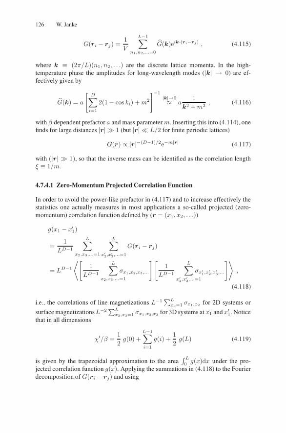
126 W. Janke

G(ri − rj) =1V

L−1∑n1,n2,...=0

G(k)eik·(ri−rj) , (4.115)

where k ≡ (2π/L)(n1, n2, . . .) are the discrete lattice momenta. In the high-temperature phase the amplitudes for long-wavelength modes (|k| → 0) are ef-fectively given by

G(k) = a

[D∑i=1

2(1− cos ki) +m2

]−1|k|→0≈ a

1k2 +m2

, (4.116)

with β dependent prefactor a and mass parameterm. Inserting this into (4.114), onefinds for large distances |r| � 1 (but |r| � L/2 for finite periodic lattices)

G(r) ∝ |r|−(D−1)/2e−m|r| (4.117)

with (|r| � 1), so that the inverse mass can be identified as the correlation lengthξ ≡ 1/m.

4.7.4.1 Zero-Momentum Projected Correlation Function

In order to avoid the power-like prefactor in (4.117) and to increase effectively thestatistics one actually measures in most applications a so-called projected (zero-momentum) correlation function defined by (r = (x1, x2, . . .))

g(x1 − x′1)

=1

LD−1

L∑x2,x3,...=1

L∑x′2,x

′3,...=1

G(ri − rj)

= LD−1

⟨[1

LD−1

L∑x2,x3,...=1

σx1,x2,x3,...

] [1

LD−1

L∑x′2,x

′3,...=1

σx′1,x

′2,x

′3,...

]⟩,

(4.118)

i.e., the correlations of line magnetizations L−1∑Lx2=1 σx1,x2 for 2D systems or

surface magnetizationsL−2∑Lx2,x3=1 σx1,x2,x3 for 3D systems at x1 and x′1. Notice

that in all dimensions

χ′/β =12g(0) +

L−1∑i=1

g(i) +12g(L) (4.119)

is given by the trapezoidal approximation to the area∫ L0g(x)dx under the pro-

jected correlation function g(x). Applying the summations in (4.118) to the Fourierdecomposition of G(ri − rj) and using


1LD−1

L∑x2,x3,...=1

eik2x2+ik3x3+... = δk2,0 δk3,0 . . . , (4.120)

it is easy to see that

g(x1 − x′1) =a

L

L−1∑n1=0

eik1(x1−x′1)

2(1− cos k1) +m2(4.121)

is the one-dimensional version of (4.115) and (4.116), since all but one momentumcomponent are projected to zero in (4.120). This can be evaluated exactly as

g(x) =a

2 sinhm∗cosh[m∗(L/2− x)]

sinh(m∗L/2)

=a

2 sinhm∗

[e−m

∗x +2e−m

∗L

1− e−m∗L cosh(m∗x)], (4.122)

with m and m∗ related by

m

2= sinh

(m∗

2

),

m∗

2= ln

[m

2+

√(m2

)2

+ 1

]. (4.123)

For ξ > 10 (m < 0.1) the difference between ξ and ξ∗ ≡ 1/m∗ is completelynegligible, (ξ∗ − ξ)/ξ < 0.042%. Notice that there is no x-dependent prefactor in(4.122). And also note that G(r) computed for r along one of the coordinate axesis a truly D-dimensional correlation function (albeit along some special direction),exhibiting the r(D−1)/2 prefactor of (4.117).

Figure 4.14 shows as an example g(x) for the standard nn Ising model atT = 2.5 ≈ 1.1 Tc on a 50×50 square lattice. By fitting the Monte Carlo datato the cosh-form (4.122), m∗ = 0.167 9 is obtained or ξ∗ = 5.957. Insertingthis value into (4.123), one obtains ξ = 1/m = 5.950. This is in very goodagreement (at a 0.1-0.2% level) with the exactly known correlation length (of thetwo-dimensional correlation function) along one of the two main coordinate axes,ξ(ex)|| = −1/(ln(tanh(β)) + 2β) = 5.962 376 984 . . . [14, 15].

4.7.4.2 Second-Moment Correlation Length

Alternatively, one may also measure directly the Fourier amplitudes

G(k) =∑

r

G(r)e−ik·r =1V〈|σ(k)|2〉 , (4.124)

for a few long-wavelength modes σ(k) =∑

r σ(r)eik·r , where the normalizationis chosen such that G(0) = χ′/β. From (4.116) we read off that

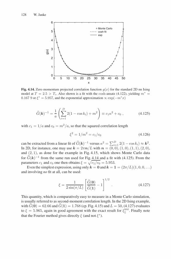
128 W. Janke

0 5 10 15 20 25 30 35 40 45 50x

0

1

2

3

4

5

6

g(x)

Monte Carlocosh fitexp

Fig. 4.14. Zero momentum projected correlation function g(x) for the standard 2D nn Isingmodel at T = 2.5 > Tc. Also shown is a fit with the cosh-ansatz (4.122), yielding m∗ =0.167 9 or ξ∗ = 5.957, and the exponential approximation ∝ exp(−m∗x)

G(k)−1 =1a

(D∑i=1

2(1− cos ki) +m2

)≡ c1κ2 + c0 , (4.125)

with c1 = 1/a and c0 = m2/a, so that the squared correlation length

ξ2 = 1/m2 = c1/c0 (4.126)

can be extracted from a linear fit of G(k)−1 versus κ2 =∑D

i=1 2(1− coski) ≈ k2.In 2D, for instance, one may use k = 2πn/L with n = (0, 0), (1, 0), (1, 1), (2, 0),and (2, 1), as done for the example in Fig. 4.15, which shows Monte Carlo datafor G(k)−1 from the same run used for Fig. 4.14 and a fit with (4.125). From theparameters c1 and c0 one then obtains ξ =

√c1/c0 = 5.953.

Even the simplest expression, using only k = 0 and k = 1 = (2π/L)(1, 0, 0, . . .)and involving no fit at all, can be used:

ξ =1

2 sin(π/L)

[G(0)

G(1)− 1

]1/2

. (4.127)

This quantity, which is comparatively easy to measure in a Monte Carlo simulation,is usually referred to as second-moment correlation length. In the 2D Ising example,with G(0) = 62.66 and G(1) = 1.768 (cp. Fig. 4.15) andL = 50, (4.127) evaluatesto ξ = 5.965, again in good agreement with the exact result for ξ(ex)

|| . Finally notethat the Fourier method gives directly ξ (and not ξ∗).


0.00 0.02 0.04 0.06 0.080.00

0.01

0.02

0.03

0.04

0.05

0.06

0.07

0.08

1/G

(k)

Monte Carlofit

Σi=12(1 − cos ki)2

Fig. 4.15. Inverse long-wavelength Fourier components G(k)−1 versus squared lattice mo-menta κ2 ≡ ∑2

i=1 2(1 − cos ki) ≈ k2 for the 2D Ising model at T = 2.5 > Tc. Thefit (4.125), c1κ

2 + c0, gives c1 = 0.565 5 and c0 = 0.015 96, and hence by (4.126),ξ =

√c1/c0 = 5.953

4.8 Generalized Ensemble Methods

All Monte Carlo methods described so far assumed a conventional canonical ensem-ble where the probability distribution of configurations is governed by a Boltzmannfactor∝ exp(−βE). A simulation at some inverse temperature β0 then covers a cer-tain range of configuration space but not all (recall the discussion of the reweightingrange). In principle a broader range can be achieved by patching several simula-tions at different temperatures using the multi-histogram method. Loosely speakinggeneralized ensemble methods aim at replacing this static patching by a single simu-lation in an appropriately defined generalized ensemble. The purpose of this sectionis to give at least a brief survey of the available methods.

4.8.1 Simulated Tempering

One approach are tempering methods which may be characterized as dynamicalmulti-histogramming. Similarly to the static reweighting approach, in simulated aswell as in parallel tempering one considers m simulation points β1 < β2 < . . . <βm which here, however, are combined already during the simulation in a specific,dynamical way.

In simulated tempering simulations [142, 143] one starts from a joint partitionfunction (expanded ensemble)

ZST =m∑i=1

egi

∑{σ}

e−βiH({σ}) , (4.128)

130 W. Janke

where gi = βif(βi) and the inverse temperatureβ is treated as an additional dynam-ical degree of freedom that can take the values β1, . . . , βm. Employing a Metropolisalgorithm, a proposed move from β = βi to βj is accepted with probability

W = min [1, exp[−(βj − βi)H({σ})] + gj − gi] . (4.129)

Similar to multi-histogram reweighting (and also to multicanonical simulations), thefree-energy parameters gi are a priori unknown and have to be adjusted iteratively.To assure a reasonable acceptance rate for the β-update moves (usually betweenneighboring βi-values), the histograms at βi and βi+1, i = 1, . . . ,m − 1, mustoverlap. An estimate for a suitable spacing δβ = βi+1 − βi of the simulation pointsβi is hence immediately given by the results (4.82)–(4.84) for the reweighting range,

δβ ∝

⎧⎪⎨⎪⎩L−D/2 off-critical

L−1/ν critical

L−D first-order

. (4.130)

Overall the simulated tempering method shows some similarities to the avoiding-rare-events variant of multicanonical simulations briefly discussed in the nextsubsection.

4.8.2 Parallel Tempering

In parallel tempering (replica exchange Monte Carlo, multiple Markov chain MonteCarlo) simulations [144, 145, 146], the starting point is a product of partition func-tions (extended ensemble),

ZPT =m∏i=1

Z(βi) =m∏i=1

∑{σ}i

e−βiH({σ}i) , (4.131)

and all m systems at different simulation points β1 < β2 < . . . < βm are sim-ulated in parallel, using any legitimate update algorithm (Metropolis, cluster,. . . ).This freedom in the choice of update algorithm is a big advantage of the paral-lel tempering method. After a certain number of sweeps, exchanges of the cur-rent configurations {σ}i and {σ}j are attempted (equivalently, the βi may be ex-changed, as is done in most implementations). Adapting the Metropolis criterion(4.24) to the present situation, the proposed exchange will be accepted with proba-bility W = min(1, eΔ), where

Δ = (βj − βi) [E({σ}j)− E({σ}i)] . (4.132)

To assure a reasonable acceptance rate, usually only nearest-neighbor exchanges(j = i ± 1) are attempted and the βi should again be spaced with the δβ given in(4.130). In most applications, the smallest inverse temperature β1 is chosen in thehigh-temperature phase where the autocorrelation time is expected to be very shortand the system decorrelates rapidly. Conceptually this approach follows again theavoiding-rare-events strategy.

Notice that in parallel tempering no free-energy parameters have to be adjusted.The method is thus very flexible and moreover can be almost trivially parallelized.


4.8.3 Multicanonical Ensembles

To conclude this introduction to simulation techniques, at least a very brief outlineof multicanonical ensembles shall be given. For more details, in particular on practi-cal implementations, see the recent reviews [4, 147, 148, 149, 150]. Similarly to thetempering methods of the last section, multicanonical simulations may also be in-terpreted as a dynamical multi-histogram reweighting method. This interpretation isstressed by the notation used in the original papers by Berg and Neuhaus [151, 152]and explains the name multicanonical. At the same time, this method may also beviewed as a specific realization of non-Boltzmann sampling [153] which has beenknown since long to be a legitimate alternative to the more standard Monte Carlo ap-proaches [154]. The practical significance of non-Boltzmann sampling was first re-alized in the so-called umbrella-sampling method [155, 156, 157], but it took manyyears before the introduction of the multicanonical ensemble [151, 152] turned non-Boltzmann sampling into a widely appreciated practical tool in computer simulationstudies of phase transitions. Once the feasibility of such a generalized ensemble ap-proach was realized, many related methods and further refinements were developed.

Conceptually the method can be divided into two main strategies. The first strat-egy can be best described as avoiding rare events which is close in spirit to thealternative tempering methods. In this variant one tries to connect the importantparts of phase space by easy paths which go around suppressed rare-event regionswhich hence cannot be studied directly. The second approach is based on enhanc-ing the probability of rare event states, which is for example the typical strategy fordealing with the highly suppressed mixed-phase region of first-order phase transi-tions [47, 150]. This allows a direct study of properties of the rare-event states suchas, e.g., interface tensions or more generally free energy barriers, which would bevery difficult (or practically impossible) with canonical simulations and also withthe tempering methods described in Sects. 4.8.1 and 4.8.2.

In general the idea is as follows. With {σ} representing generically the degreesof freedom (discrete spins or continuous field variables), the canonical Boltzmanndistribution

Pcan({σ}) ∝ e−βH({σ}) (4.133)

is replaced by an auxiliary multicanonical distribution

Pmuca({σ}) ∝W (Q({σ}))e−βH({σ}) ≡ e−βHmuca({σ}) , (4.134)

introducing a multicanonical weight factor W (Q) where Q stands for any macro-scopic observable such as the energy or magnetization. This defines formallyHmuca = H− (1/β) lnW (Q) which may be interpreted as an effective multicanon-ical Hamiltonian. The Monte Carlo sampling can then be implemented as usual bycomparingHmuca before and after a proposed update of {σ}, and canonical expec-tation values can be recovered exactly by inverse reweighting

〈O〉can = 〈OW−1(Q)〉muca/〈W−1(Q)〉muca (4.135)

132 W. Janke

similarly to (4.89). The goal is now to find a suitable weight factor W such that thedynamics of the multicanonical simulation profits most.

To be specific, let us assume in the following that the relevant macroscopic ob-servable is the energy E itself. This is for instance the case at a temperature drivenfirst-order phase transition, where the canonical energy distribution Pcan(E) devel-ops a characteristic double-peak structure [47]. As an illustration, simulation datafor the 2D seven-state Potts model [158] are shown in Fig. 4.16. With increasingsystem size, the region between the two peaks becomes more and more suppressed(∝ exp(−2σodLD−1) where σod is the (reduced) interface tension, LD−1 the cross-section of aD-dimensional system, and the factor two accounts for the fact that withthe usually employed periodic boundary condition at least two interfaces are presentdue to topological reasons) and the autocorrelation time thus grows exponentiallywith the system size L. In the literature, this is sometimes termed supercritical slow-ing down (even though nothing is critical here). Given such a situation, one usuallyadjusts W = W (E) such that the multicanonical distribution Pmuca(E) is approx-imately constant between the two peaks of Pcan(E), thus aiming at a random-walk(pseudo-) dynamics of the Monte Carlo process, cf. Fig. 4.16.

The crucial non-trivial point is, of course, how this can be achieved. On a pieceof paper,W (E) ∝ 1/Pcan(E) – but we do not know Pcan(E) (otherwise there wouldbe little need for the simulation . . . ). The solution of this problem is a recursivecomputation. Starting with the canonical distribution, or some initial guess basedon results for already simulated smaller systems together with finite-size scaling

1.0 1.2 1.4 1.6

−E/V

0.0

1.0

2.0

3.0

P(E

)

q = 7, L = 60

Pmuca

Pcan

Fig. 4.16. The canonical energy density Pcan(E) of the 2D 7-state Potts model on a 60×60lattice at inverse temperature βeqh,L, where the two peaks are of equal height, together withthe multicanonical energy density Pmuca(E), which is approximately constant between thetwo peaks


extrapolations, one performs a relatively short simulation to get an improved esti-mate of the canonical distribution. When this is inverted one obtains a new estimateof the multicanonical weight factor, which then is used in the next iteration and soon. In this naive variant only the simulation data of the last iteration are used in theconstruction of the improved weight factor.

A more sophisticated recursion, in which the updated weight factor, or moreconveniently the ratioR(E) = W (E+ΔE)/W (E), is computed from all availabledata accumulated so far, works as follows [159]:

(i) Perform a simulation with Rn(E) to obtain the nth histogram Hn(E).(ii) Compute the statistical weight of the nth run:

p(E) = Hn(E)Hn(E +ΔE)/[Hn(E) +Hn(E +ΔE)] . (4.136)

(iii) Accumulate statistics:

pn+1(E) = pn(E) + p(E) ,κ(E) = p(E)/pn+1(E) .

(4.137)

(iv) Update weight ratios:

Rn+1(E) = Rn(E) [Hn(E)/Hn(E +ΔE)]κ(E) . (4.138)

Go to (i).

The recursion is initialized with p0(E) = 0. To derive this recursion one as-sumes that (unnormalized) histogram entriesHn(E) have an a priori statistical error√Hn(E) and (quite crudely) that all data are uncorrelated. Due to the accumulation

of statistics, this procedure is rather insensitive to the length of the nth run in the firststep and has proved to be rather stable and efficient in practice.

In most applications local update algorithms have been employed, but for certainclasses of models also non-local multigrid methods [119, 120, 160, 161] are appli-cable [121, 162]. A combination with non-local cluster update algorithms, on theother hand, is not straightforward. Only by making direct use of the random-clusterrepresentation as a starting point, a multibondic variant [163, 164, 165] has been de-veloped. For a recent application to improved finite-size scaling studies of second-order phase transitions, see [128]. If Pmuca was completely flat and the Monte Carloupdate moves would perform an ideal random walk, one would expect that after V 2

local updates the system has travelled on average a distance V in total energy. Sinceone lattice sweep consists of V local updates, the autocorrelation time should scalein this idealized picture as τ ∝ V . Numerical tests for various models with a first-order phase transition have shown that in practice the data are at best consistent witha behavior τ ∝ V α, with α ≥ 1. While for the temperature-driven transitions of 2DPotts models the multibondic variant seems to saturate the bound [163, 164, 165],employing local update algorithms, typical fit results are α ≈ 1.1–1.3, and due tothe limited accuracy of the data even a weak exponential growth law cannot reallybe excluded.

134 W. Janke

In fact, at least for the field-driven first-order transition of the 2D Ising modelbelow Tc, where one works with the magnetization instead of the energy (some-times called multimagnetical simulations), it has been demonstrated recently [166]that even for a perfectly flat multicanonical distribution there are two hidden freeenergy barriers (in directions orthogonal to the magnetization) which lead to an ex-ponential growth of τ with lattice size, which is albeit much weaker than the leadingsupercritical slowing down of the canonical simulation. Physically the two barriersare related to the nucleation of a large droplet of the wrong phase (say down-spins inthe background of up-spins) [167, 168, 169, 170, 171, 172, 173] and the transitionof this large, more or less spherical droplet to the strip phase (coexisting strips ofdown- and up-spins, separated by two straight interfaces) aroundm = 0 [174].

4.8.4 Wang-Landau Recursion

Another more recently proposed method deals directly with estimators Ω(E) of thedensity of states [175, 176]. By flipping spins randomly, the transition probabilityfrom energy level E1 to E2 is

p(E1 → E2) = min[Ω(E1)Ω(E2)

, 1]. (4.139)

Each time an energy level is visited, the estimator is multiplicatively updated

Ω(E)→ f Ω(E) , (4.140)

where initially Ω(E) = 1 and f = f0 = e1. Once the accumulated energy his-togram is sufficiently flat, the factor f is refined

fn+1 =√fn (4.141)

with n = 0, 1, . . ., and the energy histogram reset to zero until some small valuesuch as f = e10−8 ≈ 1.000 000 01 is reached.

For the 2D Ising model this procedure converges very rapidly towards the ex-actly known density of states, and also for other applications a fast convergence hasbeen reported. Since the procedure is known to violate detailed balance, however,some care is necessary in setting up a proper protocol of the recursion. Most authorswho employ the obtained density of states directly to extract canonical expectationvalues by standard reweighting argue that, once f is close enough to unity, sys-tematic deviations become negligible. While this claim can be verified empiricallyfor the 2D Ising model (where exact results are available for judgement), possiblesystematic deviations are difficult to assess in the general case. A safe way wouldbe to consider the recursion (4.139)–(4.141) as an alternative method to determinethe multicanonical weights, and then to perform a usual multicanonical simulationbased on them. As emphasized earlier, any deviations of multicanonical weightsfrom their optimal shape do not show up in the final canonical expectation values;they rather only influence the dynamics of the multicanonical simulations.


4.9 Concluding Remarks

The intention of these lecture notes was to give an elementary introduction to theconcepts of modern Markov chain Monte Carlo simulations and to illustrate theirusefulness by applications to the very simple Ising lattice spin model. The basicMonte Carlo methods employing local update rules are straightforward to generalizeto all models with discrete degrees of freedom and, with small restrictions, also to allmodels with continuous variables and off-lattice systems. Non-local cluster updatemethods are much more efficient but also more specialized. Some generalizations toPotts and O(n) symmetric spin models have been indicated and also further modelsmay be efficiently simulated by this method, but there is no guarantee that for a givenmodel a cluster update procedure can be developed. The statistical error analysis isobviously completely general, and also the example finite-size scaling analysis canbe taken as a guideline for any model exhibiting a second-order phase transition.Finally, reweighting techniques and generalized ensemble ideas such as temperingmethods, the multicanonical ensemble and Wang-Landau sampling can be adaptedto almost every statistical physics problem at hand once the relevant macroscopicobservables are identified.

Acknowledgements

Many people have influenced these lecture notes with their advice, discussions,questions, and active contributions. In particular I wish to thank Michael Bachmann,Bertrand Berche, Pierre-Emmanuel Berche, Bernd A. Berg, Alain Billoire, KurtBinder, Elmar Bittner, Christophe Chatelain, Thomas Haase, Malte Henkel,Desmond A. Johnston, Christoph Junghans, Ralph Kenna, David P. Landau, EricLorenz, Thomas Neuhaus, Andreas Nußbaumer, Michel Pleimling, Adriaan Schakel,and Martin Weigel for sharing their insight and knowledge with me. Special thanksgo to Elmar Bittner for his help with the sample finite-size scaling analysis.

This work was partially supported by the Deutsche Forschungsgemeinschaft(DFG) under grants JA 483/22-1 and JA 483/23-1, the EU RTN-Network “EN-RAGE”: Random Geometry and Random Matrices: From Quantum Gravity toEconophysics under grant MRTN-CT-2004-005616, and the JUMP computer timegrants hlz10, hlz11, and hlz12 of NIC at Forschungszentrum Julich.

References

1. M. Newman, G. Barkema, Monte Carlo Methods in Statistical Physics (ClarendonPress, Oxford, 1999) 80, 86

2. D. Landau, K. Binder, Monte Carlo Simulations in Statistical Physics (Cambridge Uni-versity Press, Cambridge, 2000) 80, 86

3. K. Binder, D. Heermann, Monte Carlo Simulations in Statistical Physics: An Introduc-tion, 4th edn. (Springer, Berlin, 2002) 80, 86

136 W. Janke

4. B. Berg, Markov Chain Monte Carlo Simulations and Their Statistical Analysis (WorldScientific, Singapore, 2004) 80, 86, 131

5. H. Stanley, Introduction to Phase Transitions and Critical Phenomena (Oxford Press,Oxford, 1979) 80, 92

6. J. Binney, N. Dowrick, A. Fisher, M. Newman, The Theory of Critical Phenomena(Oxford University Press, Oxford, 1992) 80

7. D. Lavis, G. Bell, Statistical Mechanics of Lattice Systems 2 (Springer, Berlin, 1999) 808. C. Domb, J. Lebowitz (eds.), Phase Transitions and Critical Phenomena (Academic

Press, New York, 1976) 809. W. Lenz, Phys. Z. 21, 613 (1920) 81

10. E. Ising, Phys. Z. 31, 253 (1925) 8111. L. Onsager, Phys. Rev. 65, 117 (1944) 8212. B. Kaufman, Phys. Rev. 76, 1232 (1949) 82, 10913. A. Ferdinand, M. Fisher, Phys. Rev. 185, 832 (1969) 82, 10914. B. McCoy, T. Wu, The Two-Dimensional Ising Model (Harvard University Press,

Cambridge, 1973) 82, 12715. R. Baxter, Exactly Solved Models in Statistical Mechanics (Academic Press, New York,

1982) 82, 12716. L. Onsager, Nuovo Cimento 6, 261 (1949) 8217. C. Yang, Phys. Rev. 85, 808 (1952) 8218. C. Chang, Phys. Rev. 88, 1422 (1952) 8219. W. Orrick, B. Nickel, A. Guttmann, J. Perk, Phys. Rev. Lett. 86, 4120 (2001) 8220. W. Orrick, B. Nickel, A. Guttmann, J. Perk, J. Stat. Phys. 102, 795 (2001) 8221. R. Griffiths, Phys. Rev. Lett. 24, 1479 (1970) 8322. G. Rushbrooke, J. Chem. Phys. 39, 842 (1963) 8323. R. Griffiths, Phys. Rev. Lett. 14, 623 (1965) 8324. B. Josephson, Proc. Phys. Soc. 92, 269 (1967) 8325. B. Josephson, Proc. Phys. Soc. 92, 276 (1967) 8326. M. Fisher, Phys. Rev. 180, 594 (1969) 8327. L. Widom, J. Chem. Phys. 43, 3892 (1965) 8328. L. Widom, J. Chem. Phys. 43, 3898 (1965) 8329. L. Kadanoff, Physics 2, 263 (1966) 8330. K. Wilson, J. Kogut, Phys. Rep. C12, 75 (1974) 8331. F. Wu, Rev. Mod. Phys. 54, 235 (1982) 8432. F. Wu, Rev. Mod. Phys. 55, 315(E) (1983) 8433. M. Weigel, W. Janke, Phys. Rev. B62, 6343 (2000) 8434. K. Binder, in Monte Carlo Methods in Statistical Physics ed. by K. Binder (Springer,

Berlin, 1979), p. 1 84, 8635. M. Barber, in Phase Transitions and Critical Phenomena, Vol. 8 ed. by C. Domb,

J. Lebowitz (Academic Press, New York, 1983), p. 146 8436. V. Privman (ed.), Finite-Size Scaling and Numerical Simulations of Statistical Systems

(World Scientific, Singapore, 1990) 8437. K. Binder: in Computational Methods in Field Theory, Schladming Lecture Notes, eds.

H. Gausterer, C.B. Lang (Springer, Berlin, 1992), P. 59 8438. J. Gunton, M. Miguel, P. Sahni, in Phase Transitions and Critical Phenomena, Vol. 8,

ed. by C. Domb, J. Lebowitz (Academic Press, New York, 1983) 8539. K. Binder, Rep. Prog. Phys. 50, 783 (1987) 8540. H. Herrmann, W. Janke, F. Karsch (eds.), Dynamics of First Order Phase Transitions

(World Scientific, Singapore, 1992) 85


41. W. Janke, in Computer Simulations in Condensed Matter Physics, Vol. VII, ed. byD. Landau, K. Mon, H.B. Schuttler (Springer, Berlin, 1994), p. 29 85

42. M. Fisher, A. Berker, Phys. Rev. B 26, 2507 (1982) 8543. V. Privman, M. Fisher, J. Stat. Phys. 33, 385 (1983) 8544. K. Binder, D. Landau, Phys. Rev. B 30, 1477 (1984) 8545. M. Challa, D. Landau, K. Binder, Phys. Rev. B 34, 1841 (1986) 8546. V. Privman, J. Rudnik, J. Stat. Phys. 60, 551 (1990) 8547. W. Janke, in Computer Simulations of Surfaces and Interfaces, NATO Science Series,

II. Mathematics, Physics and Chemistry Vol. 114, ed. by B. Dunweg, D. Landau,A. Milchev (Kluwer, Dordrecht, 2003), pp. 111–135 85, 92, 111, 131, 132

48. C. Borgs, R. Kotecky J. Stat. Phys. 61, 79 (1990) 8549. J. Lee, J. Kosterlitz Phys. Rev. Lett. 65, 137 (1990) 8550. C. Borgs, R. Kotecky, S. Miracle-Sole, J. Stat. Phys. 62, 529 (1991) 8551. C. Borgs, W. Janke, Phys. Rev. Lett. 68, 1738 (1992) 8552. W. Janke, Phys. Rev. B 47, 14757 (1993) 8553. J. Hammersley, D. Handscomb, Monte Carlo Methods (Chapman and Hall, London,

New York, 1964) 8554. D. Heermann, Computer Simulation Methods in Theoretical Physics, 2nd edn.

(Springer, Berlin, 1990) 8655. K. Binder (ed.), The Monte Carlo Method in Condensed Matter Physics (Springer,

Berlin, 1992) 8656. N. Metropolis, A. Rosenbluth, M. Rosenbluth, A. Teller, E. Teller, J. Chem. Phys. 21,

1087 (1953) 8657. S. Kirkpatrick, C. Gelatt. Jr., M. Vecchi, Science 220, 671 (1983) 8758. W. Janke, in Ageing and the Glass Transition – Summer School, University of Lux-

embourg, September 2005, Lecture Notes in Physics, Vol. 716, ed. by M. Henkel,M. Pleimling, R. Sanctuary (Springer, Berlin, Heidelberg, 2007), Lecture Notes inPhysics, pp. 207–260 87, 89, 103, 106

59. W. Janke, in Proceedings of the Euro Winter School Quantum Simulations of Com-plex Many-Body Systems: From Theory to Algorithms, NIC Series, Vol. 10, ed. byJ. Grotendorst, D. Marx, A. Muramatsu (John von Neumann Institute for Computing,Julich, 2002), pp. 447–458 87

60. R. Glauber, J. Math. Phys. 4, 294 (1963) 89, 9061. R. Swendsen, J.S. Wang, Phys. Rev. Lett. 58, 86 (1987) 93, 94, 9762. R. Potts, Proc. Camb. Phil. Soc. 48, 106 (1952) 9363. U. Wolff, Phys. Rev. Lett. 62, 361 (1989) 93, 94, 9664. W. Janke, Mathematics and Computers in Simulations 47, 329 (1998) 9365. P. Kasteleyn, C. Fortuin, J. Phys. Soc. Japan 26, 11 (1969) 9366. C. Fortuin, P. Kasteleyn, Physica 57, 536 (1972) 9367. C. Fortuin, Physica 58, 393 (1972) 9368. C. Fortuin, Physica 59, 545 (1972) 9369. U. Wolff, Nucl. Phys. B322, 759 (1989) 96, 9870. M. Hasenbusch, Nucl. Phys. B333, 581 (1990) 9671. U. Wolff, Nucl. Phys. B334, 581 (1990) 96, 97, 9872. U. Wolff, Phys. Lett. A 228, 379 (1989) 96, 9773. C. Baillie, Int. J. Mod. Phys. C 1, 91 (1990) 9674. M. Hasenbusch, S. Meyer, Phys. Lett. B 241, 238 (1990) 9675. R. Swendsen, J.S. Wang, A. Ferrenberg, in The Monte Carlo Method in Condensed

Matter Physics ed. by K. Binder (Springer, Berlin, 1992) 96

138 W. Janke

76. X.L. Li, A. Sokal, Phys. Rev. Lett. 63, 827 (1989) 9677. X.L. Li, A. Sokal, Phys. Rev. Lett. 67, 1482 (1991) 9678. M. Nightingale, H. Blote, Phys. Rev. Lett. 76, 4548 (1996) 97, 10079. M. Nightingale, H. Blote, Phys. Rev. B 62, 1089 (2000) 97, 10080. P. Grassberger, Physica A 214, 547 (1995) 9781. P. Grassberger, Physica A 217, 227 (E) (1995) 9782. N. Ito, K. Hukushima, K. Ogawa, Y. Ozeki, J. Phys. Soc. Japan 69, 1931 (2000) 9783. D. Heermann, A. Burkitt, Physica A 162, 210 (1990) 9784. P. Tamayo, Physica A 201, 543 (1993) 9785. N. Ito, G. Kohring, Physica A 201, 547 (1993) 9786. W. Janke, Phys. Lett. A 148, 306 (1990) 9887. C. Holm, W. Janke, Phys. Rev. B 48, 936 (1993) 98, 11388. W. Janke, A. Schakel, Nucl. Phys. B700, 385 (2004) 9889. W. Janke, A. Schakel, Comp. Phys. Comm. 169, 222 (2005) 9890. W. Janke, A. Schakel, Phys. Rev. E 71, 036703 (2005) 9891. W. Janke, A. Schakel, Phys. Rev. Lett. 95, 135702 (2005) 9892. W. Janke, A. Schakel, in Order, Disorder and Criticality: Advanced Problems of Phase

Transition Theory, Vol. 2, ed. by Y. Holovatch (World Scientific, Singapore, 2007),pp. 123–180 98

93. E. Lorenz, Ageing phenomena in phase-ordering kinetics in Potts models. Diplomathesis, Universitat Leipzig (2005). www.physik.uni-leipzig.de/∼lorenz/ diplom.pdf 100, 101

94. A. Rutenberg, A. Bray, Phys. Rev. E 51, 5499 (1995) 100, 10195. P. Calabrese, A. Gambassi, J. Phys. A 38, R133 (2005) 10096. C. Godreche, J.M. Luck, J. Phys.: Condens. Matter 14, 1589 (2002) 100, 10197. L.F. Cugliandolo: in Slow Relaxation and Non Equilibrium Dynamics in Condensed

Matter, Les Houches Lectures, eds. J.-L. Barrat, J. Dalibard, J. Kurchan, M.V.Feigel’man (Springer, Berlin, 2003) 100

98. F. Corberi, E. Lippiello, M. Zannetti, Phys. Rev. Lett. 90, 099601 (2003) 10199. M. Henkel, M. Pleimling, Phys. Rev. Lett. 90, 099602 (2003) 101

100. L. Berthier, J. Barrat, J. Kurchan, Europhys. J. B 11, 635 (1999) 101101. F. Corberi, E. Lippiello, M. Zannetti, Europhys. J. B 24, 359 (2001) 101102. F. Corberi, E. Lippiello, M. Zannetti, Phys. Rev. E 65, 046136 (2003) 101103. A. Barrat, Phys. Rev. E 57, 3629 (1998) 101104. M. Henkel, Conformal Invariance and Critical Phenomena (Springer, Berlin, 1999) 101105. M. Henkel, M. Pleimling, C. Godreche, J.M. Luck, Phys. Rev. Lett. 87, 265701 (2001)

101106. M. Henkel, Nucl. Phys. B641, 405 (2002) 101107. M. Henkel, M. Paessens, M. Pleimling, Europhys. Lett. 62, 664 (2003) 101108. M. Henkel, M. Pleimling, Phys. Rev. E 68, 065101 (R) (2003) 101109. M. Henkel, A. Picone, M. Pleimling, Europhys. Lett. 68, 191 (2004) 101110. E. Lorenz, W. Janke, Europhys. Lett. 77, 10003 (2007) 101111. W. Janke, in Proceedings of the Euro Winter School Quantum Simulations of Complex

Many-Body Systems: From Theory to Algorithms, NIC Series, Vol. 10, ed. by J. Gro-tendorst, D. Marx, A. Muramatsu (John von Neumann Institute for Computing, Julich,2002), pp. 423–445 102, 103

112. P. Beale, Phys. Rev. Lett. 76, 78 (1996) 109113. W. Press, S. Teukolsky, W. Vetterling, B. Flannery, Numerical Recipes in Fortran 77

– The Art of Scientific Computing, 2nd edn. (Cambridge University Press, Cambridge,1999) 102, 117, 120, 121


114. M. Priestley, Spectral Analysis and Time Series, Vol. 2 (Academic, London, 1981).Chaps. 5–7 103

115. T. Anderson, The Statistical Analysis of Time Series (Wiley, New York, 1971) 103116. N. Madras, A. Sokal, J. Stat. Phys. 50, 109 (1988) 103, 105117. A. Sokal, L. Thomas, J. Stat. Phys. 54, 797 (1989) 103118. A. Ferrenberg, D. Landau, K. Binder, J. Stat. Phys. 63, 867 (1991) 104119. A. Sokal, Monte Carlo Methods in Statistical Mechanics: Foundations and New Algo-

rithms (Cours de Troisieme Cycle de la Physique en Suisse Romande, Lausanne, 1989)105, 133

120. A. Sokal, in Quantum Fields on the Computer, ed. by M. Creutz (World Scientific,Singapore, 1992), p. 211 105, 133

121. W. Janke, T. Sauer, J. Stat. Phys. 78, 759 (1995) 106, 133122. B. Efron, The Jackknife, the Bootstrap and Other Resampling Plans (Society for Indus-

trial and Applied Mathematics [SIAM], Philadelphia, 1982) 107123. R. Miller, Biometrika 61, 1 (1974) 107124. A. Ferrenberg, R. Swendsen, Phys. Rev. Lett. 61, 2635 (1988) 108125. A. Ferrenberg, R. Swendsen, Phys. Rev. Lett. 63, 1658(E) (1989) 108126. N. Wilding, in Computer Simulations of Surfaces and Interfaces, NATO Science Series,

II. Mathematics, Physics and Chemistry Vol. 114, ed. by B. Dunweg, D. Landau,A. Milchev (Kluwer, Dordrecht, 2003), pp. 161–171 110

127. A. Ferrenberg, R. Swendsen, Phys. Rev. Lett. 63, 1195 (1989) 112128. B. Berg, W. Janke, Phys. Rev. Lett. 98, 040602 (2007) 114, 133129. G. Kamieniarz, H. Blote, J. Phys. A 26, 201 (1993) 116, 123130. J. Salas, A. Sokal, J. Stat. Phys. 98, 551 (2000) 116, 123131. X. Chen, V. Dohm, Phys. Rev. E 70, 056136 (2004) 116, 123132. V. Dohm, J. Phys. A 39, L259 (2006) 116, 123133. W. Selke, L. Shchur, J. Phys. A 38, L739 (2005) 116, 123134. M. Schulte, C. Drope, Int. J. Mod. Phys. C 16, 1217 (2005) 116, 123135. M. Sumour, D. Stauffer, M. Shabat, A. El-Astal, Physica A 368, 96 (2006) 116, 123136. W. Selke, Europhys. J. B 51, 223 (2006); preprint http://arxiv.org/abs/

cond-mat/0701515 116, 123137. A. Nußbaumer, E. Bittner, W. Janke, Europhys. Lett. 78, 16004 (2007) 118, 119, 123, 124138. E. Bittner, W. Janke, The pain of example analyses – a (self-)critical discussion. Un-

published results 119, 124139. W. Janke, R. Villanova, Phys. Rev. B 66, 134208 (2002) 119, 120140. J. Oitmaa, J. Phys. A 14, 1159 (1981) 121141. C. Holm, W. Janke, Phys. Rev. Lett. 78, 2265 (1997) 124142. E. Marinari, G. Parisi, Europhys. Lett. 19, 451 (1992) 129143. A. Lyubartsev, A. Martsinovski, S. Shevkunov, P. Vorontsov-Velyaminov, J. Chem.

Phys. 96, 1776 (1992) 129144. C. Geyer, in Proceedings of the 23rd Symposium on the Interface, ed. by E. Keramidas

(Interface Foundation, Fairfax, Virginia, 1991), pp. 156–163 130145. C. Geyer, E. Thompson, J. Am. Stat. Assoc. 90, 909 (1995) 130146. K. Hukushima, K. Nemoto, J. Phys. Soc. Japan 65, 1604 (1996) 130147. B. Berg, Fields Inst. Comm. 26, 1 (2000) 131148. B. Berg, Comp. Phys. Comm. 104, 52 (2002) 131149. W. Janke, Physica A 254, 164 (1998) 131150. W. Janke, in Computer Simulations of Surfaces and Interfaces, NATO Science Series, II.

Mathematics, Physics and Chemistry –Proceedings of the NATO Advanced Study Insti-tute, Albena, Bulgaria, 9–20 September 2002, Vol. 114, ed. by B. Dunweg, D. Landau,A. Milchev (Kluwer, Dordrecht, 2003) 131

140 W. Janke

151. B. Berg, T. Neuhaus, Phys. Lett. B 267, 249 (1991) 131152. B. Berg, T. Neuhaus, Phys. Rev. Lett. 68, 9 (1992) 131153. W. Janke, Int. J. Mod. Phys. C 3, 1137 (1992) 131154. K. Binder: in Phase Transitions and Critical Phenomena, Vol. 5b, eds. C. Domb, M.S.

Green (Academic Press, New York, 1976), p. 1 131155. G. Torrie, J. Valleau, Chem. Phys. Lett. 28, 578 (1974) 131156. G. Torrie, J. Valleau, J. Comp. Phys. 23, 187 (1977) 131157. G. Torrie, J. Valleau, J. Chem. Phys. 66, 1402 (1977) 131158. W. Janke, B. Berg, M. Katoot, Nucl. Phys. B382, 649 (1992) 132159. B. Berg, W. Janke. Unpublished notes 133160. J. Goodman, A. Sokal, Phys. Rev. Lett. 56, 1015 (1986) 133161. J. Goodman, A. Sokal, Phys. Rev. D 40, 2035 (1989) 133162. W. Janke, T. Sauer, Phys. Rev. E 49, 3475 (1994) 133163. W. Janke, S. Kappler, Nucl. Phys. (proc suppl.) B42, 876 (1995) 133164. W. Janke, S. Kappler, Phys. Rev. Lett. 74, 212 (1995) 133165. M. Carroll, W. Janke, S. Kappler, J. Stat. Phys. 90, 1277 (1998) 133166. T. Neuhaus, J. Hager, J. Stat. Phys. 113, 47 (2003) 134167. K. Binder, M. Kalos, J. Stat. Phys. 22, 363 (1980) 134168. H. Furukawa, K. Binder, Phys. Rev. A 26, 556 (1982) 134169. M. Biskup, L. Chayes, R. Kotecky, Europhys. Lett. 60, 21 (2002) 134170. M. Biskup, L. Chayes, R. Kotecky, Comm. Math. Phys. 242, 137 (2003) 134171. M. Biskup, L. Chayes, R. Kotecky, J. Stat. Phys. 116, 175 (2003) 134172. K. Binder, Physica A 319, 99 (2003) 134173. A. Nußbaumer, E. Bittner, T. Neuhaus, W. Janke, Europhys. Lett. 75, 716 (2006) 134174. K. Leung, R. Zia, J. Phys. A 23, 4593 (1990) 134175. F. Wang, D. Landau, Phys. Rev. Lett. 86, 2050 (2001) 134176. F. Wang, D. Landau, Phys. Rev. E 64, 056101 (2001) 134

4 monte carlo methods in classical statistical physics - institut für

Documents