4 statistical techniques - osbornebooksshop.co.uk · 4 statistical techniques this chapter...

Statistical techniques4

this chapter covers...

In this chapter we will explain how to calculate key statistical indicators which will helpus to analyse past data and help us forecast what may happen in the future.We will start by examining time series – strings of data that occur over time. We willsee how a formula can be used to represent a straight line on a graph (regressionanalysis), and how this can be used to predict data at various points. Next we will see how some data moves in regular cycles over time, and how this,together with the underlying trend can be used to develop forecasts. We will show howaveraging techniques can be used to detect the trend in given data.The third section concerns the use of index numbers. These can be used to comparenumerical data over time – for example prices of commodities or general price inflation.We will see how to carry out various calculations using index numbers that can beuseful.Finally we will briefly see how index numbers can be used to analyse standard costingvariances so that we can determine performance more accurately.

T IME SER IES ANALYS IS

Time series analysis involves analysing numerical trends over a time period.It is often used to examine past and present trends so that future trends canbe forecast. The term ‘trend analysis’ is used to describe the technique thatwe will now examine. At its simplest the concept is based on the assumptionthat data will continue to move in the same direction in the future as it has inthe past.Using the sales of a shoe shop as an example we will now look at a range oftechniques for dealing with trends.

a n i d e n t i c a l a n n u a l c h a n g eA shoe shop ‘Comfy Feet’ has sold the following numbers of pairs of shoesannually over the last few years:

20-1 10,00020-2 11,00020-3 12,00020-4 13,00020-5 14,00020-6 15,00020-7 16,000

It does not require a great deal of arithmetic to calculate that if the trendcontinues at the previous rate – an increase of 1,000 pairs a year – then shoesales could be forecast at 17,000 pairs in 20-8 and 18,000 pairs in 20-9. Ofcourse this is a very simple example, and life is rarely this straightforward.For example, for how long can this rate of increase be sustained?

a v e r a g e a n n u a l c h a n g eA slightly more complex technique could have been used to arrive at thesame answer for the shoe shop. If we compare the number of sales in 20-7with the number in 20-1, we can see that it has risen by 6,000 pairs. Bydividing that figure by the number of times the year changed in our data wecan arrive at an average change per year. The number of times that the yearchanges is 6, which is the same as the number of ‘spaces’ between the years(or alternatively the total number of years minus 1).Shown as an equation this becomes:Average Annual Sales Change = (Sales in Last Year – Sales in First Year) = (16,000 – 10,000) (Number of Years – 1) (7 – 1)

= + 1,000, which is what we would expect.

s t a t i s t i c a l t e c h n i q u e s 1 2 5

The + 1,000 would then be added to the sales data in 20-7 of 16,000 (the lastactual data) to arrive at a forecast of 17,000.This technique is useful when all the increases are not quite identical, yet wewant to use the average increase to forecast the trend. A negative answerwould show that the average change is a reduction, not an increase. We willuse this technique when estimating the trend movement in more complicatedsituations.This is not the only way that we can estimate the direction that data ismoving over time, and it does depend on the data (including especially thefirst and last points) falling roughly into a straight line. We will notealternative methods that can be used later in this section.

c o n s t r u c t i n g a g r a p hThe same result can be produced graphically. Using the same shoe shopexample we can extend the graph based on the actual data to form a forecastline.

If in another situation the actual data does not produce exactly equal increases,the graph will produce the same answer as the average annual change providedthe straight line runs through the first and last year’s data points.

1 2 6 m a n a g e m e n t a c c o u n t i n g : d e c i s i o n a n d c o n t r o l t u t o r i a l

forecast dataComfy Feet: Sales of shoes

20-1

20-2

20-3

20-4

20-5

20-7

20-8

20-9

20-6


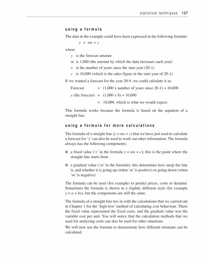
u s i n g a f o r m u l aThe data in the example could have been expressed in the following formula:

y = mx + cwhere y is the forecast amount m is 1,000 (the amount by which the data increases each year) x is the number of years since the start year (20-1) c is 10,000 (which is the sales figure in the start year of 20-1)If we wanted a forecast for the year 20-9, we could calculate it as: Forecast = (1,000 x number of years since 20-1) + 10,000 y (the forecast) = (1,000 x 8) + 10,000 = 18,000, which is what we would expect.This formula works because the formula is based on the equation of astraight line.

u s i n g a f o r m u l a f o r m o r e c a l c u l a t i o n sThe formula of a straight line (y = mx + c) that we have just used to calculatea forecast for ‘y’ can also be used to work out other information. The formulaalways has the following components:n a fixed value (‘c’ in the formula y = mx + c); this is the point where the

straight line starts fromn a gradient value (‘m’ in the formula); this determines how steep the line

is, and whether it is going up (when ‘m’ is positive) or going down (when‘m’ is negative)

The formula can be used (for example) to predict prices, costs or demand.Sometimes the formula is shown in a slightly different style (for example y = a + bx), but the components are still the same.The formula of a straight line ties in with the calculations that we carried outin Chapter 1 for the ‘high-low’ method of calculating cost behaviour. Therethe fixed value represented the fixed costs, and the gradient value was thevariable cost per unit. You will notice that the calculation methods that weused for analysing costs can also be used for other situations.We will now use the formula to demonstrate how different elements can becalculated.

Just like in the high-low method, if you are provided with more than twopairs of data, then using the highest and the lowest will probably give themost reliable answer.We will now use an example to illustrate the use of the formula to predictdemand.


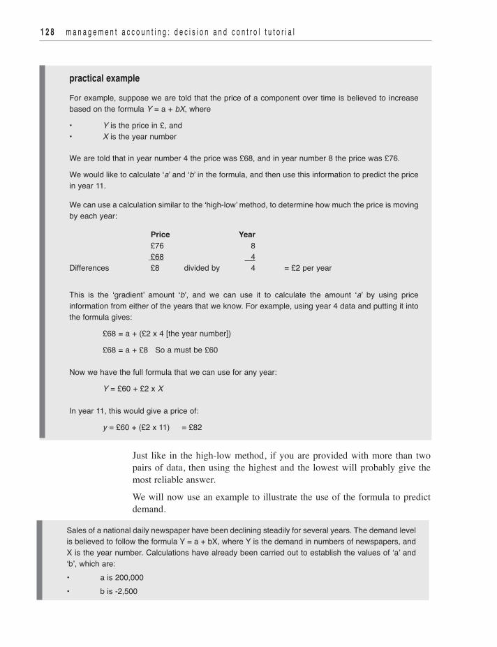
practical exampleFor example, suppose we are told that the price of a component over time is believed to increasebased on the formula Y = a + bX, where

• Y is the price in £, and• X is the year number

We are told that in year number 4 the price was £68, and in year number 8 the price was £76.

We would like to calculate ‘a’ and ‘b’ in the formula, and then use this information to predict the pricein year 11.

We can use a calculation similar to the ‘high-low’ method, to determine how much the price is movingby each year:

Price Year£76 8 £68 4

Differences £8 divided by 4 = £2 per year

This is the ‘gradient’ amount ‘b’, and we can use it to calculate the amount ‘a’ by using priceinformation from either of the years that we know. For example, using year 4 data and putting it intothe formula gives:

£68 = a + (£2 x 4 [the year number])

£68 = a + £8 So a must be £60

Now we have the full formula that we can use for any year:

Y = £60 + £2 x X

In year 11, this would give a price of:

y = £60 + (£2 x 11) = £82

Sales of a national daily newspaper have been declining steadily for several years. The demand levelis believed to follow the formula Y = a + bX, where Y is the demand in numbers of newspapers, andX is the year number. Calculations have already been carried out to establish the values of ‘a’ and‘b’, which are:• a is 200,000• b is -2,500


l i n e a r r e g r e s s i o n

In the last section on time series analysis we saw that when some historicaldata moves in a consistent and regular way over time we can use it to helpestimate the future trend of that data. We also saw that in thesecircumstances the data can be represented byn a straight line on a graph, and / or n an equation of the line in the form y = mx + cto help us develop the trend.Linear regression is the term used for the techniques that can be used todetermine the line that best replicates that given data. You should be awareof the techniques in general terms, and be able to appreciate their usefulness.You may be given historical data or the equation of a line and asked to use itto generate a forecast. Where data exactly matches a straight line (as with the ‘Comfy Feet’ data)there is no need to use any special techniques. In other situations thefollowing could be used:n Average annual change. This method was described earlier, and is

useful if we are confident that the first and last points (takenchronologically since we are looking at data over time) are bothrepresentative. It will smooth out any minor fluctuations of the data inbetween. We will see this method used in the ‘Seasonal Company’ casestudy later in this chapter.

n Line of best fit. Where the data falls only roughly into a straight line, butthe first and last points do not appear to be very representative theaverage annual change method would give a distorted solution. Here aline of best fit can be drawn onto the data points on a graph that will forma better estimate of the movement of the data. The graph on the next pageillustrates a situation where the line of best fit would provide a bettersolution than the average annual change method.

Note that ‘b’ is a negative figure, so each year the demand decreases.

You are asked to calculate the expected sales in year 14.

If we insert the known data into the formula, we can calculate the demand for year 14 as follows:

Y = 200,000 – (2,500 x 14) Y = 165,000

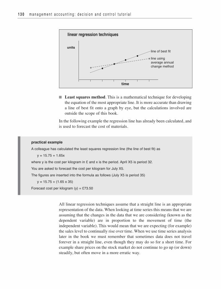
n Least squares method. This is a mathematical technique for developingthe equation of the most appropriate line. It is more accurate than drawinga line of best fit onto a graph by eye, but the calculations involved areoutside the scope of this book.

In the following example the regression line has already been calculated, andis used to forecast the cost of materials.

All linear regression techniques assume that a straight line is an appropriaterepresentation of the data. When looking at time series this means that we areassuming that the changes in the data that we are considering (known as thedependent variable) are in proportion to the movement of time (theindependent variable). This would mean that we are expecting (for example)the sales level to continually rise over time. When we use time series analysislater in the book we must remember that sometimes data does not travelforever in a straight line, even though they may do so for a short time. Forexample share prices on the stock market do not continue to go up (or down)steadily, but often move in a more erratic way.


units

time

line of best fit

line usingaverage annualchange method

linear regression techniques

practical exampleA colleague has calculated the least squares regression line (the line of best fit) as

y = 15.75 + 1.65xwhere y is the cost per kilogram in £ and x is the period. April X5 is period 32.You are asked to forecast the cost per kilogram for July X5.The figures are inserted into the formula as follows (July X5 is period 35)

y = 15.75 + (1.65 x 35) Forecast cost per kilogram (y) = £73.50


T IME SER IES ANALYS IS AND SEASONAL VAR IAT IONS

There are four main factors that can influence data which is generated overa period of time:n The underlying trend

This is the way that the data is generally moving in the long term. Forexample the volume of traffic on our roads is generally increasing as timegoes on.

n Long term cyclesThese are slow moving variations that may be caused by economic cyclesor social trends. For example, when economic prosperity generallyincreases this may increase the volume of traffic as more people own carsand fewer use buses. In times of economic depression there may be adecrease in car use as people cannot afford to travel as much or may nothave employment which requires them to travel.

n Seasonal variationsThis term refers to regular, predictable cycles in the data. The cycles mayor may not be seasonal in the normal use of the term (eg Spring, Summeretc). For example traffic volumes are always higher in the daytime,especially on weekdays, and lower at weekends and at night.

n Random variationsAll data will be affected by influences that are unpredictable. Forexample flooding of some roads may reduce traffic volume along thatroute, but increase it on alternative routes. Similarly the traffic volumemay be influenced by heavy snowfall.

The type of numerical problems that you are most likely to face will tend toignore the effects of long-term cycles (which will effectively be consideredas a part of the trend) and random variations (which are impossible toforecast). We are therefore left with analysing data into underlying trendsand seasonal variations, in order to create forecasts.The technique that we will use follows the process in the diagram on the nextpage.

The process is as follows:1 The historical actual data is analysed into the historical trend and the

seasonal variations.2 The historical trend is used to forecast the future trend, using the

techniques examined in the last section.

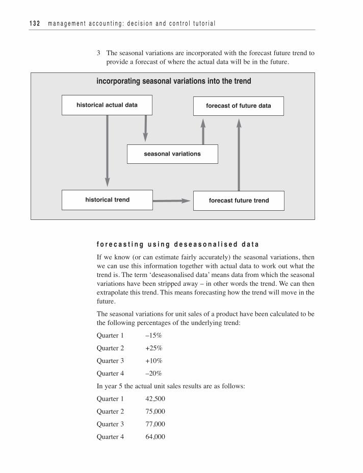
3 The seasonal variations are incorporated with the forecast future trend toprovide a forecast of where the actual data will be in the future.

f o r e c a s t i n g u s i n g d e s e a s o n a l i s e d d a t aIf we know (or can estimate fairly accurately) the seasonal variations, thenwe can use this information together with actual data to work out what thetrend is. The term ‘deseasonalised data’ means data from which the seasonalvariations have been stripped away – in other words the trend. We can thenextrapolate this trend. This means forecasting how the trend will move in thefuture.The seasonal variations for unit sales of a product have been calculated to bethe following percentages of the underlying trend:Quarter 1 –15%Quarter 2 +25%Quarter 3 +10%Quarter 4 –20%In year 5 the actual unit sales results are as follows:Quarter 1 42,500Quarter 2 75,000Quarter 3 77,000Quarter 4 64,000


incorporating seasonal variations into the trend

historical actual data forecast of future data

historical trend forecast future trend

seasonal variations


From these figures we can calculate the ‘deseasonalised’ data – the trendfigures. We need to be careful because the seasonal variations are calculatedas percentages of the trend.

Quarter 1 The trend must be greater than 42,500 by 15% of the trend.Therefore 42,500 must equal 85% of the trendTrend = 42,500 x 100 / 85 = 50,000

Quarter 2 The trend must be lower than 75,000 by 25% of the trend.Therefore 75,000 must equal 125% of the trendTrend = 75,000 x 100 / 125 = 60,000

Using the same logic:

Quarter 3 Trend = 77,000 x 100 / 110 = 70,000

Quarter 4 Trend = 64,000 x 100 / 80 = 80,000

Having identified the trend for year 5 as 50,000, 60,000, 70,000 and 80,000we can see that it is rising by 10,000 units per quarter. Therefore the forecastfor year 6 can be worked out as follows:

Year 6 Quarter 1 Quarter 2 Quarter 3 Quarter 4

Extrapolated Trend 90,000 100,000 110,000 120,000

Seasonal Variations –15% +25% +10% –20%

Forecast 76,500 125,000 121,000 96,000

In a task the analysis of actual data may have been carried out already, or youmay be asked to carry out the analysis by using ‘moving averages’. If youare using moving averages it is important that: n your workings are laid out accurately n the number of pieces of data that are averaged corresponds with the

number of ‘seasons’ in a cyclen where there is an even number of ‘seasons’ in a cycle a further averaging

of each pair of averages takes place

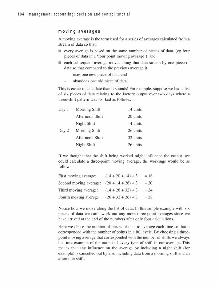
mo v i n g a v e r a g e sA moving average is the term used for a series of averages calculated from astream of data so that: n every average is based on the same number of pieces of data, (eg four

pieces of data in a ‘four point moving average’), andn each subsequent average moves along that data stream by one piece of

data so that compared to the previous average it– uses one new piece of data and– abandons one old piece of data.

This is easier to calculate than it sounds! For example, suppose we had a listof six pieces of data relating to the factory output over two days where athree-shift pattern was worked as follows:

Day 1 Morning Shift 14 units Afternoon Shift 20 units Night Shift 14 units

Day 2 Morning Shift 26 units Afternoon Shift 32 units Night Shift 26 units

If we thought that the shift being worked might influence the output, wecould calculate a three-point moving average, the workings would be asfollows:

First moving average: (14 + 20 + 14) ÷ 3 = 16Second moving average: (20 + 14 + 26) ÷ 3 = 20Third moving average: (14 + 26 + 32) ÷ 3 = 24Fourth moving average (26 + 32 + 26) ÷ 3 = 28

Notice how we move along the list of data. In this simple example with sixpieces of data we can’t work out any more three-point averages since wehave arrived at the end of the numbers after only four calculations.Here we chose the number of pieces of data to average each time so that itcorresponded with the number of points in a full cycle. By choosing a three-point moving average that corresponded with the number of shifts we alwayshad one example of the output of every type of shift in our average. Thismeans that any influence on the average by including a night shift (forexample) is cancelled out by also including data from a morning shift and anafternoon shift.


We must be careful to always work out moving averages so that exactly onecomplete cycle is included in every average. The number of ‘points’ ischosen to suit the data.When determining a trend line, each average relates to the data from its midpoint, as the following layout of the figures just calculated demonstrates.

Output Trend (Moving Average)Day 1 Morning Shift 14 units Afternoon Shift 20 units 16 units Night Shift 14 units 20 unitsDay 2 Morning Shift 26 units 24 units Afternoon Shift 32 units 28 units Night Shift 26 units

This means that the first average that we calculated (16 units) can be used asthe trend point of the afternoon shift on day 1, with the second point (20units) forming the trend point of the night shift on day 1. The result is thatwe:n know exactly where the trend line is for each period of time, andn have a basis from which we can calculate ‘seasonal variations’Even using our limited data in this example we can see how seasonalvariations can be calculated. A seasonal variation is simply the differencebetween the actual data at a point and the trend at the same point. Thisgives us the seasonal variations shown in the following table, using thefigures already calculated.

Output Trend Seasonal VariationDay 1 Morning Shift 14 units Afternoon Shift 20 units 16 units + 4 units Night Shift 14 units 20 units - 6 unitsDay 2 Morning Shift 26 units 24 units + 2 units Afternoon Shift 32 units 28 units + 4 units Night Shift 26 units

The seasonal variation for the afternoon shift, calculated on day 1, is basedon the actual output being 4 units greater than the trend at the same point (20minus 16 units).



CaseStudy

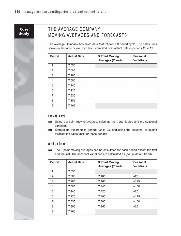
THE AVERAGE COMPANYMOV ING AVERAGES AND FORECASTSThe Average Company has sales data that follows a 3 period cycle. The sales unitsshown in the table below have been compiled from actual data in periods 11 to 19.

Period Actual Data 3 Point Moving Seasonal Averages (Trend) Variations11 7,650 12 7,505 13 7,285 14 7,590 15 7,445 16 7,225 17 7,530 18 7,385 19 7,165

r e q u i r e d(a) Using a 3 point moving average, calculate the trend figures and the seasonal

variations(b) Extrapolate the trend to periods 20 to 25, and using the seasonal variations

forecast the sales units for those periods

s o l u t i o n(a) The 3 point moving averages can be calculated for each period except the first

and the last. The seasonal variations are calculated as (actual data – trend).

Period Actual Data 3 Point Moving Seasonal Averages (Trend) Variations11 7,650 12 7,505 7,480 +2513 7,285 7,460 –17514 7,590 7,440 +15015 7,445 7,420 +2516 7,225 7,400 –17517 7,530 7,380 +15018 7,385 7,360 +2519 7,165

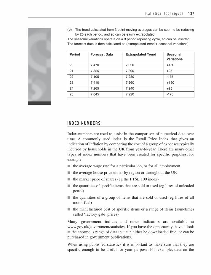
(b) The trend calculated from 3 point moving averages can be seen to be reducingby 20 each period, and so can be easily extrapolated.

The seasonal variations operate on a 3 period repeating cycle, so can be inserted. The forecast data is then calculated as (extrapolated trend + seasonal variations).

Period Forecast Data Extrapolated Trend Seasonal Variations20 7,470 7,320 +15021 7,325 7,300 +2522 7,105 7,280 -17523 7,410 7,260 +15024 7,265 7,240 +2525 7,045 7,220 -175

I NDEX NUMBERS

Index numbers are used to assist in the comparison of numerical data overtime. A commonly used index is the Retail Price Index that gives anindication of inflation by comparing the cost of a group of expenses typicallyincurred by households in the UK from year-to-year. There are many othertypes of index numbers that have been created for specific purposes, forexample:n the average wage rate for a particular job, or for all employmentn the average house price either by region or throughout the UKn the market price of shares (eg the FTSE 100 index)n the quantities of specific items that are sold or used (eg litres of unleaded

petrol)n the quantities of a group of items that are sold or used (eg litres of all

motor fuel)n the manufactured cost of specific items or a range of items (sometimes

called ‘factory gate’ prices)Many government indices and other indicators are available atwww.gov.uk/government/statistics. If you have the opportunity, have a lookat the enormous range of data that can either be downloaded free, or can bepurchased in government publications. When using published statistics it is important to make sure that they arespecific enough to be useful for your purpose. For example, data on the


growth in the population of the West of England will be of limited use if youare trying to forecast the sales in a bookshop in Taunton. Of far more usewould be details of proposed housing developments within the immediatearea, including the numbers of new homes and the type of households thatform the developers’ target market.

l e a d i n g a n d l a g g i n g i n d i c a t o r sSome indicators can be classified as ‘leading’ indicators, whilst others areknown as ‘lagging’ indicators. This means that some indicators naturallygive advance warning of changes that may take place later in otherindicators. For example an index that monitors the prices of manufacturedgoods (‘factory gate’ prices) will react to changes before they have filteredthrough to retail price indices. The index of ‘factory gate’ prices cantherefore be considered to be a ‘leading’ indicator of retail prices, and giveearly warning of implications to industrial situations.In a similar way, an index recording the volume of manufactured output fromfactories will lag behind an index measuring the volume of purchases of rawmaterials made by industrial buying departments.

w e i g h t i n g s o f i n d i c e sThose indices that are based on information from more than one item willuse some form of weighting to make the results meaningful. For example while an index measuring the retail price of premium gradeunleaded petrol is based on a single product and therefore needs noweighting, this would not be true for a price index for all vehicle fuel. In thiscase it will require a decision about how much weight (or importance) is tobe placed on each component of the index. Here the relative quantities soldof types of fuel (for example unleaded petrol and diesel) would be a logicalway to weight the index. This would ensure that if petrol sales were doublethose for diesel, any price changes in petrol would have twice the impact onthe index than a price change in diesel.As the purchasing habits of consumers change, then the weighting andcomposition of complicated indices like the Retail Price Index and theConsumer Price Index are often changed to reflect this. This will includechanges to the weighting of certain items, for example due to the increase inthe proportion of household expenditure on holidays. It can also involve theaddition or deletion of certain items entirely (for example the inclusion ofcertain fast foods). You may have seen news items from time to time aboutthe revision of items contained within the RPI or CPI as consumers’ tasteschange.


c a l c u l a t i o n s u s i n g i n d e x n u m b e r sWhatever type of index we need to use, the principle is the same. The indexnumbers represent a convenient way of comparing figures. For example, the RPI was 82.61 in January 1983, and 245.8 in January 2013.This means that average household costs had nearly tripled in the 30 yearsbetween. We could also calculate that if something that cost £5.00 in January1983 had risen exactly in line with inflation, it would have cost £14.88 inJanuary 2013. This calculation is carried out by:

historical price x index of time converting to index of time converting fromie £5.00 x (245.8 ÷ 82.61) = £14.88

This is an increase of (£14.88 – £5.00) x 100 = 197.6%£5.00

You may be told that the ‘base year’ for a particular index is a certain pointin time. This is when the particular index was 100. For example the currentRPI index was 100 in January 1987. Index numbers referring to costs or prices are the most commonly used onesreferred to in the unit studied in this book. If we want to use cost indexnumbers to monitor past costs or forecast future ones, then it is best to use asspecific an index as possible. This will then provide greater accuracy than amore general index.For example, if we were operating in the food industry, and wanted tocompare our coffee cost movements with the average that the industry hadexperienced, we should use an index that analyses coffee costs in the foodindustry. This would be much more accurate than the RPI, and also betterthan a general cost index for the food industry.


p r a c t i c a l e x a m p l eThe following table shows the actual material costs for January for years 20X2 to 20X5, together withthe relevant price index.

Period Actual costs (£) Cost index Costs at January 20X2 pricesJanuary 20X2 129,300 471 January 20X3 131,230 482 January 20X4 135,100 490 January 20X5 136,250 495

Required: Restate all the actual costs at January 20X2 prices, to the nearest £.

TURNER L IM I TED : ADJUST ING TO REAL TERMSSales revenue and Net Profit figures are given for Turner Ltd for the five years ended31 December 20-1 to 20-5. A suitable index for Turner Ltd’s industry is also given.

20-1 20-2 20-3 20-4 20-5Sales revenue (£000s) 435 450 464 468 475Net Profit (£000s) 65 70 72 75 78Industry Index 133 135 138 140 143

r e q u i r e dCalculate the sales revenue and profit in terms of year 20-5 values and comment onthe results.

s o l u t i o nTo put each figure into 20-5 terms, it is divided by the index for its own year andmultiplied by the index for 20-5, ie 143. For example:

Sales revenue Year 20-1 435 x 143 = 467.7 133

Sales revenue Year 20-2 450 x 143 = 476.7 and so on. 135

In year 20-5 terms: 20-1 20-2 20-3 20-4 20-5Sales revenue (£000s) 467.7 476.7 480.8 478.0 475.0Net Profit (£000s) 69.9 74.1 74.6 76.6 78.0

The adjusted figures compare like with like in terms of the value of the pound, and theNet Profit still shows an increasing trend throughout, but the sales revenue decreasesin the last two years.


Solution

Period Actual costs (£) Cost index Costs at January 20X2 pricesJanuary 20X2 129,300 471 129,300January 20X3 131,230 482 128,235January 20X4 135,100 490 129,861January 20X5 136,250 495 129,644

CaseStudy


c r e a t i o n o f a n i n d e x

You may be required to create an index from given historical data, and wewill now see how this is carried out.Suppose that you are provided with the following prices for one unit of acertain material over a period of time:

Month Jan Feb March April May June

Price £29.70 £30.00 £28.30 £30.09 £31.00 £31.25

The first thing to do is to decide which point in time is to be the base point– the price at this point will be 100 in our new index. In this example we willfirst use January as our base point, but later we will see how another datecould have been chosen.Next, the price of another date (we’ll use February) is divided by the price atthe base point. The result is then multiplied by 100 to give the index at thatpoint (ie February):

(£30.00 / £29.70) x 100 = 101.01Note that the index number is not an amount in £s, it is just a number usedfor comparison purposes. In this example we’ve rounded to 2 decimal places– and we will need to be consistent for the other figures.

If we carry out the same calculation for the March price we get the following:(£28.30 / £29.70) x 100 = 95.29

Notice that here the answer is less than 100, which makes sense because theprice in March is lower than the price in January. Checking that each indexnumber is the expected side of 100 (ie higher or lower) is a good idea andwill help you to detect some arithmetical errors.The full list of index numbers is as follows – make sure that you can arriveat the same figures.


Price £29.70 £30.00 £28.30 £30.09 £31.00 £31.25

Index 100.00 101.01 95.29 101.31 104.38 105.22

We could have chosen a different date to act as our base point – if we choseMarch, then the calculation for January would have been:

(£29.70 / £28.30) x 100 = 104.95Then the full list of index numbers would have been as follows:


Price £29.70 £30.00 £28.30 £30.09 £31.00 £31.25

Index 104.95 106.01 100.00 106.33 109.54 110.42

Again, make sure that you could arrive at the same figures.Don’t forget that although we have used the creation of a price index in theabove example, you could also be asked to create an index from any suitablehistorical data. Whatever the type of data, the arithmetic required is the same.

US ING I NDEX NUMBERS TO ANALYSE VAR IANCES

When standard costing is being used, standards for material prices will havebeen set based on expected costs. This will often be based on an expectedlevel of a price index for that material (if there is one available). If the priceindex for the material changes significantly then we can calculate what thestandard would be if it was based on the index (the ‘revised’ standard price).We can then see how that impacts on any price variance that has beencalculated.Once we have worked out what the ‘revised’ standard price would be, we canthen calculate the part of a price variance explained by the index change as:

minus

The remainder of the original variance would be the part not explained by thechange in price index.The following case study illustrates the process.

ANALYS IS L IM I TEDREV ISED STANDARD PR ICEAnalysis Limited operates a standard costing system and uses a raw material that isa global commodity. The standard price was set based upon a market price of £950per kilo when the relevant price index was 315.In April the price index was 330. The quantity of material purchased and used was 128kilos, which cost £125,000.


the revised standadr cost ofthe actual material

the original standard cost ofthe actual material

CaseStudy

r e q u i r e d• Calculate the material price variance, based on the original standard• Calculate what the ‘revised’ standard price per kilo would be, based on the changein the index, to the nearest £

• Analyse the material price variance into the part explained by the change in theindex, and the remainder.

s o l u t i o n• The material price variance is (£950 x 128 kilos) - £125,000 = £3,400 adverse• The ‘revised’ standard price per kilo would be: £950 x 330 / 315 = £995 to the nearest £• The part of the price variance explained by the index change: (£950 x 128 kilos) – (£995 x 128 kilos) = £5,760 adverse

The remainder of the variance is therefore: £3,400 adverse minus £5,760 adverse = £2,260 favourable

In this situation the price actually paid for material is lower than would be expectedfrom the change in the index.

n A time series is formed by data that occurs over time. If the data increasesor decreases regularly (in a ‘straight line’) then it can be represented by aformula. The formula can then be used to predict the data at various points.

n Some data moves in regular cycles over time, and the distances that thedata is from the underlying trend are known as seasonal variations.Information about the underlying trend and the seasonal variations can beused to forecast data.

n Moving averages can be used to split data into the trend and the seasonalvariations.

n Index numbers can be used to compare numerical data over time.Examples of the use of index numbers are for prices of commodities orgeneral price inflation.

n Index numbers can be used to analyse standard costing variances so thatwe can determine performance more accurately.


ChapterSummary

time series analysis the examination of historical data that occursover time, often with the intention of using thedata to forecast future data

trend the underlying movement in the data, onceseasonal and random movements have beenstripped away

seasonal variations regular variations in data that occur in arepeating pattern

extrapolation of data using information about a known range of datato predict data outside the range (for example inthe future)

deseasonalised data data that has had seasonal variations strippedaway

linear regression using a mathematical formula to demonstratethe movement of data over time. This techniqueis sometimes used to help forecast themovement of the trend

index numbers a sequence of numbers used to compare data,usually over a time period


KeyTerms

4.1 Sales (in units) of a product are changing at a steady rate and don’t seem to be affected by anyseasonal variations. Use the data given for the first three periods to forecast the sales for periods4 and 5.

Period 1 2 3 4 5

Sales (units) 212,800 210,600 208,400

Activities


4.2 Sales (in units) of a product are changing at a broadly steady rate and don’t seem to be affectedby any seasonal variations. Use the average change in the data given for the first five periods toforecast the sales for periods 6 and 7.

Period 1 2 3 4 5 6 7

Sales (units) 123,400 123,970 124,525 125,085 125,640

4.3 The table below shows the last three months cost per kilo for material Beta, together with estimatedseasonal variations:

Month Jan Feb March April May

Actual Price £ 6.80 6.40 7.00

Seasonal Variation £ +0.40 –0.10 +0.40 –0.30 –0.40

Trend £

• Calculate the trend figures for January to March, and extrapolate them to April and May.

• Forecast the actual prices in April and May

4.4 Computer modelling has been used to identify the regression formula for the monthly total of aspecific indirect cost as

Y = £13.20 x + £480.00Where y is total monthly costAnd x is monthly production in units

Calculate the total monthly cost when output is

• 500 units, and

• 800 units

State whether the total cost behaves as a

• Fixed cost, or

• Variable cost, or

• Semi-variable cost, or

• Stepped cost.

4.5 The regression formula for monthly sales of a certain product (in units) has been identified as:Y = 1,200 + 13XWhere Y is total monthly sales, and X is the month number.January 20X9 was month 30

Forecast the monthly sales in August 20X9

4.6 A company has sales data that follows a 3 period cycle. The sales units shown in the table belowhave been compiled from actual data in periods 30 to 36.

Period Actual Data 3 Point Moving Seasonal Averages (Trend) Variations

30 3,500

31 3,430

32 3,450

33 3,530

34 3,460

35 3,480

36 3,560

37

38

39

40

Complete the table to show your responses to the following:

(a) Using a 3 point moving average, calculate the trend figures and the seasonal variations forperiods 31 to 35

(b) Extrapolate the trend to periods 37 to 40, and using the seasonal variations forecast thesales units for those periods


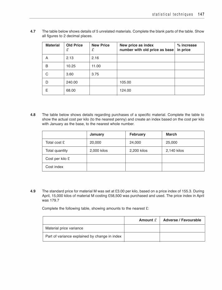
4.7 The table below shows details of 5 unrelated materials. Complete the blank parts of the table. Showall figures to 2 decimal places.

Material Old Price New Price New price as index % increase £ £ number with old price as base in price

A 2.13 2.16

B 10.25 11.00

C 3.60 3.75

D 240.00 105.00

E 68.00 124.00

4.8 The table below shows details regarding purchases of a specific material. Complete the table toshow the actual cost per kilo (to the nearest penny) and create an index based on the cost per kilowith January as the base, to the nearest whole number.

January February March

Total cost £ 20,000 24,000 25,000

Total quantity 2,000 kilos 2,200 kilos 2,140 kilos

Cost per kilo £

Cost index

4.9 The standard price for material M was set at £3.00 per kilo, based on a price index of 155.3. DuringApril, 15,000 kilos of material M costing £58,500 was purchased and used. The price index in Aprilwas 179.7

Complete the following table, showing amounts to the nearest £:

Amount £ Adverse / Favourable

Material price variance

Part of variance explained by change in index


4 statistical techniques - osbornebooksshop.co.uk · 4 statistical techniques this chapter...

Documents