4. technological progress and growth: … growth model. the general solow model ... figure 4.1: the...

Advanced Macroeconomics www.ekonomika.org

___________________________________________________________________________ 2009.12.29 Page 220 of 1314

4. TECHNOLOGICAL PROGRESS AND GROWTH: THE GENERAL SOLOW MODEL

■ In one respect the basic Solow model did not perform well empirically: its long-run balanced growth path displayed zero growth in GDP per capita. This is at odds with the observed long-run growth in living standards in Western economies. ■ We want to develop a growth model whose long-term prediction is a balanced growth path with strictly positive growth in GDP per person. Obviously we can only trust the answers to our big questions, “what creates prosperity in the long run?” and “what creates transitory and long-run growth?”, if these answers are grounded in a (growth) model that accords with the most basic empirical facts. ■ This lecture presents a growth model with the properties we are looking for: the steady state of the model exhibits balanced growth with positive growth in output per worker. We obtain this by a slight generalization of the basic Solow model. The resulting model is


___________________________________________________________________________ 2009.12.29 21 of 1314

close to the one actually suggested by Robert M. Solow in his famous 1956 article “A Contribution to the Theory of Economic Growth”, Quarterly Journal of Economics, 70, 1956. ■ The essential new feature of the model is that total factor productivity is no longer assumed to be a constant, B. Instead it will be given as an exogenous sequence, (Bt), which may be steadily growing over time. In that case the model's steady state will display balanced growth with steady positive growth in GDP per worker. ■ Hence, according to the general Solow model (as we will call it) the root of steady positive long-run growth in GDP per person is a steady exogenous technological progress. This explanation of growth may not seem deep. However, it is not trivial that the consequence of steadily arriving technological progress should be a balanced growth path, and it is reassuring for the application of the model to issues of economic policy that its steady state mirrors a robust long-run growth fact. Of course, explaining the technological progress that creates growth in GDP per worker is a matter of great interest and it is the subject of the endogenous growth theory.


___________________________________________________________________________ 2009.12.29 Page 222 of 1314

■ Having obtained in this lecture a model that fits the basic stylized growth facts better, we are going to take the model through some more specific empirical tests. The tests will focus on the steady state prediction of the model as well as its outside steady state prediction concerning transitory growth or convergence. ■ Our conclusion will be that the general Solow model does quite well empirically, both with respect to its steady state and its transitory growth predictions, although there will be some aspects still to be improved upon. The general Solow model is indeed a very important growth model. The general Solow model ■ With respect to the qualitative features of the underlying “micro world”, the general Solow model is identical to the basic Solow model. It has the same commodities and markets, and the markets are again assumed to be perfectly competitive. There are also the same kinds of economic agents, and their behaviour is essentially the same. In particular, a representative profit-maximizing firm has to decide on the inputs of capital and labour


___________________________________________________________________________ 2009.12.29 Page 223 of 1314

services, Ktd and Lt

d, in each period t, given the real rental rate of capital, rt, and the real wage rate, wt. The only difference is that the production function, which tells how much output can be produced from Kt

d and Ltd, may now change over time so that, for instance, more

and more output can be obtained from the same amounts of inputs. The production function with technological progress ■ The total factor productivity will now be allowed to depend on time. The notation for it will therefore be Bt, where Bt > 0 in all time periods t. The full time sequence, (Bt), of total factor productivity is exogenous. Maintaining a Cobb-Douglas form, the production function in period t is:

Yt = BtKtαLt

1-α, 0 < α < 1 4.1

■ This time we insert from the beginning the feature that the inputs demanded and actually used, Kt

d and Ltd, must equal the (inelastic) supplies, Kt and Lt, because the factor markets


___________________________________________________________________________ 2009.12.29 Page 224 of 1314

clear. Since one particular assumption on (Bt) could be that Bt is constant, the general Solow model, or just the Solow model, is a generalization of the basic Solow model. We may alternatively write the production function as:

Yt = Ktα(AtLt)1-α 4.2

where At ≡ Bt

1/(1-α). With the Cobb-Douglas form of the production function it makes no difference whether we describe technological change by a certain time sequence, (Bt), of the total factor productivity, or by an appropriately defined sequence, (At), of the labour productivity variable (not to be confused with the average labour productivity, Yt/Lt). ■ With more general production functions it may make some difference. Generally, technological progress that appears as an increasing variable, At, in a production function, F(Kt, AtLt), is called labour-augmenting or Harrod-neutral.


___________________________________________________________________________ 2009.12.29 Page 225 of 1314

■ If it appears as an increasing variable, Dt, in F(DtKt, Lt), it is called capital-augmenting or Solow-neutral, while, when it appears as an increasing variable, Bt, in BtF(Kt,Lt), it is called Hicks-neutral. ■ Given the Cobb-Douglas specification one can simply choose the formulation of technological progress that is most convenient. For our present purposes this turns out to be the form with labour-augmenting technological change as in (4.2). ■ A full description of the production possibilities includes a specification of the exogenous sequence, (At). We will simply assume that the labour productivity variable, At is changing at a constant rate: At+1 = (1 + g)At, g > –1 4.3


___________________________________________________________________________ 2009.12.29 Page 226 of 1314

■ Here g is the exact (not the approximate) growth rate of At. It follows that if the technological level in some initial period zero is A0, then in period t it is At = (1 + g)tA0. For the approximate growth rate, gt

A = ln At – ln At-1. ■ A positive value of g corresponds to a steadily arriving technological progress that comes exogenously to the economy without this requiring the use of economic resources. The production function just becomes ever more efficient period by period. It is sometimes said that technological progress comes as “manna from heaven”. ■ The idea of the “endogenous growth” models is to change the description of technological progress, so that it will be the outcome of a use of economic resources. ■ We will again use the definitions of output per worker (average labour productivity) yt ≡ Yt/Lt, and capital per worker (the capital intensity) kt ≡ Kt/Lt. Dividing by Lt on both sides of (4.2) gives the per capita production function: yt = kt

αAt1-α 4.4


___________________________________________________________________________ 2009.12.29 Page 227 of 1314

and then, taking logs and time differences, ln yt - ln yt-1 = α(ln kt – ln kt-1) + (1 – α)(ln At – ln At-1) 4.5 or in the usual notation for approximate growth rates: gt

y = αgtk + (1 – α)gt

A 4.6 ■ These expressions reveal that an increase in output per worker can be obtained in two ways, by more capital per worker or by better technology. ■ In fact, the (approximate) growth rate in output per worker is the weighted average of the rates of growth in capital per worker and in technology, the weights being α and (1 – α) respectively. There are now two potential sources of economic growth: capital accumulation and technological progress.


___________________________________________________________________________ 2009.12.29 Page 228 of 1314

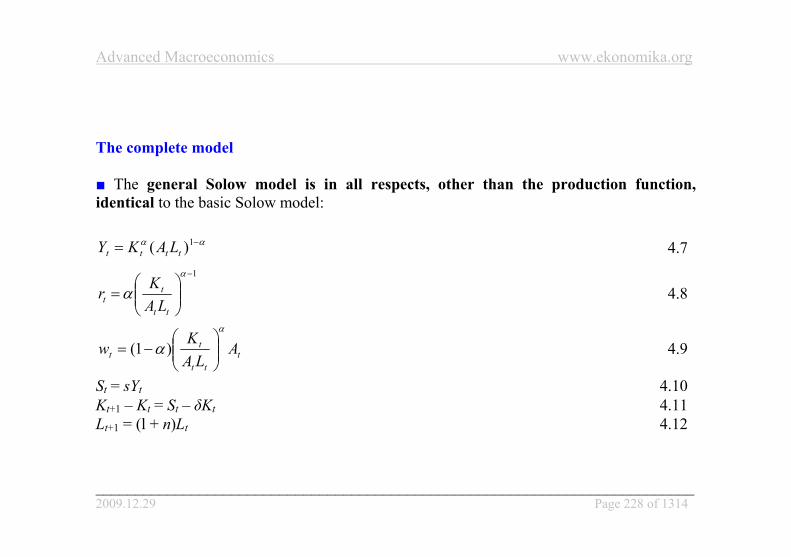
The complete model ■ The general Solow model is in all respects, other than the production function, identical to the basic Solow model:

αα −= 1)( tttt LAKY 4.71−

⎟⎟⎠

⎞⎜⎜⎝

⎛=

α

αtt

tt LA

Kr 4.8

ttt

tt A

LAKw

α

α ⎟⎟⎠

⎞⎜⎜⎝

⎛−= )1( 4.9

St = sYt 4.10Kt+1 – Kt = St – δKt 4.11Lt+1 = (l + n)Lt 4.12


___________________________________________________________________________ 2009.12.29 Page 229 of 1314

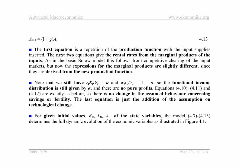
At+1 = (l + g)At 4.13 ■ The first equation is a repetition of the production function with the input supplies inserted. The next two equations give the rental rates from the marginal products of the inputs. As in the basic Solow model this follows from competitive clearing of the input markets, but now the expressions for the marginal products are slightly different, since they are derived from the new production function. ■ Note that we still have rtKt/Yt = α and wtLt/Yt = 1 – α, so the functional income distribution is still given by α, and there are no pure profits. Equations (4.10), (4.11) and (4.12) are exactly as before, so there is no change in the assumed behaviour concerning savings or fertility. The last equation is just the addition of the assumption on technological change. ■ For given initial values, K0, L0, A0, of the state variables, the model (4.7)-(4.13) determines the full dynamic evolution of the economic variables as illustrated in Figure 4.1.


___________________________________________________________________________ 2009.12.29 Page 230 of 1314

Figure 4.1: The dynamics of the general Solow model

Note: Predetermined endogenous variables in squares, endogenous variables that can adjust in the period in circles. Analysing the general Solow model ■ A first guess regarding the economic evolution implied by the general Solow model could be that, just as in the basic Solow model, the capital intensity, kt, will converge to a specific steady state value. One can see from equation (4.6) that if kt reaches a constant


___________________________________________________________________________ 2009.12.29 Page 231 of 1314

level, output per worker, yt, will be increasing approximately at the rate (1 –α)g because of technological progress. Hence, as wanted, we would have a steady state with economic growth, assuming g > 0. ■ This guess is wrong, but it is instructive to see why it is wrong, and why it is not what we want to find. First, if kt stays constant at some level, then indeed from (4.4) or (4.6), income per worker, yt, will be increasing (since g > 0), and the ever larger income per worker will create ever higher savings per worker, and eventually this will have to imply more and more capital per person. So kt cannot stay constant in the long run when g > 0. ■ Second, the growth path according to the guess, with a constant kt and an increasing yt, would not be a balanced growth path. One of the requirements of balanced growth, as defined in Lecture 2, is that kt and yt change by the same rate, so that the capital-output ratio stays constant. The general Solow model would not perform well by empirical standards if the guess had been correct.


___________________________________________________________________________ 2009.12.29 Page 232 of 1314

In the general Solow model something more subtle is going on. Let us find out what really happens. The law of motion ■ We analysed the basic Solow model in terms of the variables kt and yt which turned out to converge to specific and constant steady state levels. We also want to analyse the general Solow model in terms of variables that will be constant in steady state. As we have just seen, we cannot use kt and yt as such variables, since both have to change over time when g ≠ 0. What variables could be used? ■ For the long-run equilibrium of the model to accord with balanced growth, kt and yt should be changing at the same rate in steady state. Look again at (4.6) above. If the (approximate) growth rates of kt and yt are the same, gt

y = gtk, then (4.6) implies that their

common value has to be the approximate growth rate of At, that is, gty = gt

k = gtA.


___________________________________________________________________________ 2009.12.29 Page 233 of 1314

■ So, if the model should imply convergence on a balanced growth path, then it must also imply that the growth rates of kt and yt both converge to the exogenous growth rate of At so that eventually kt/At and yt/At will be constant. ■ This suggests analysing the model in terms of the variables:

tt

t

t

tt LA

KAkk =≡

~

tt

t

t

tt LA

YAyy =≡~

4.14

often called the technology-adjusted capital intensity (or capital per effective worker) and the technology-adjusted average labour productivity (or output per effective worker), respectively. ■ Dividing on both sides of the production function (4.7) by AtLt gives:


___________________________________________________________________________ 2009.12.29 Page 234 of 1314

α

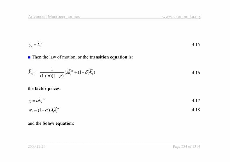
tt ky ~~ = 4.15 ■ Then the law of motion, or the transition equation is:

)~)1(~()1)(1(

1~1 ttt kks

gnk δα −+

++=+ 4.16

the factor prices:

1~ −= αα tt kr 4.17αα ttt kAw ~)1( −= 4.18

and the Solow equation:


___________________________________________________________________________ 2009.12.29 Page 235 of 1314

)~)(~()1)(1(

1~~1 tttt knggnks

gnkk +++−

++=−+ δα 4.19

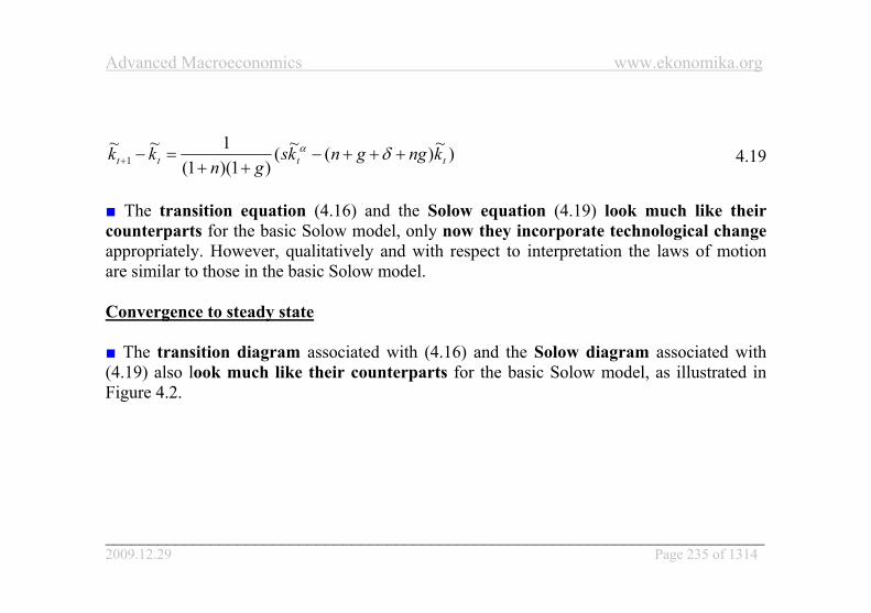
■ The transition equation (4.16) and the Solow equation (4.19) look much like their counterparts for the basic Solow model, only now they incorporate technological change appropriately. However, qualitatively and with respect to interpretation the laws of motion are similar to those in the basic Solow model. Convergence to steady state ■ The transition diagram associated with (4.16) and the Solow diagram associated with (4.19) also look much like their counterparts for the basic Solow model, as illustrated in Figure 4.2.


___________________________________________________________________________ 2009.12.29 Page 236 of 1314


___________________________________________________________________________ 2009.12.29 Page 237 of 1314

Figure 4.2: The transition diagram (top), and the Solow diagram (bottom)


___________________________________________________________________________ 2009.12.29 Page 238 of 1314

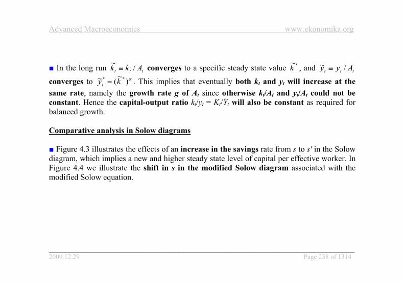
■ In the long run ttt Akk /~≡ converges to a specific steady state value *~k , and ttt Ayy /~ ≡

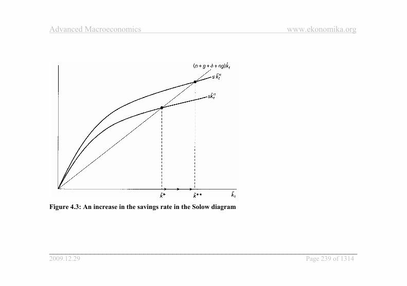
converges to α)~(~ ** kyt = . This implies that eventually both kt and yt will increase at the same rate, namely the growth rate g of At since otherwise kt/At and yt/At could not be constant. Hence the capital-output ratio kt/yt = Kt/Yt will also be constant as required for balanced growth. Comparative analysis in Solow diagrams ■ Figure 4.3 illustrates the effects of an increase in the savings rate from s to s' in the Solow diagram, which implies a new and higher steady state level of capital per effective worker. In Figure 4.4 we illustrate the shift in s in the modified Solow diagram associated with the modified Solow equation.


___________________________________________________________________________ 2009.12.29 Page 239 of 1314

Figure 4.3: An increase in the savings rate in the Solow diagram


___________________________________________________________________________ 2009.12.29 Page 240 of 1314

Figure 4.4: An increase in the savings rate in the modified Solow diagram


___________________________________________________________________________ 2009.12.29 Page 241 of 1314

■ Assume that the economy is initially in the old steady state where tk~ and ty~ are

constant and equal to *~tk and *~

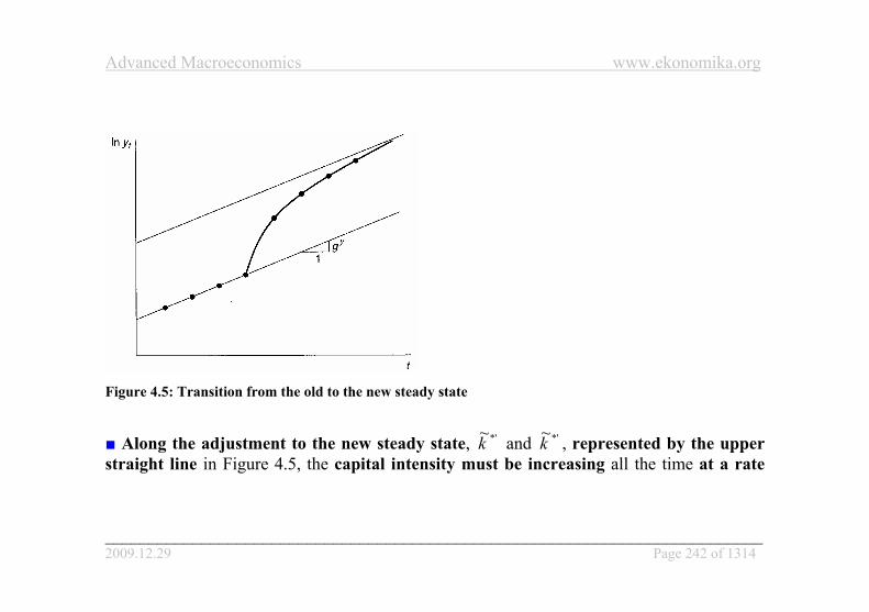
ty , respectively. In this situation capital per worker, kt, and output per worker, yt, both change over time at the rate g which we assume to be positive. The growth path corresponding to the old steady state is illustrated by the lower upward sloping straight line in Figure 4.5.


___________________________________________________________________________ 2009.12.29 Page 242 of 1314

Figure 4.5: Transition from the old to the new steady state

■ Along the adjustment to the new steady state, *'~k and *'~k , represented by the upper straight line in Figure 4.5, the capital intensity must be increasing all the time at a rate


___________________________________________________________________________ 2009.12.29 3 of 1314

which is larger than g, but gradually falls back towards g. The same must then be true for yt. The transition from the old to the new steady state is illustrated by the curve going from the lower to the upper straight line in Figure 4.5. ■ Figure 4.6 shows the adjustment of the growth rate of yt during the transition from the old to the new steady state.


___________________________________________________________________________ 2009.12.29 Page 244 of 1314

Figure 4.6: Adjustment of the growth rate during the transition


___________________________________________________________________________ 2009.12.29 Page 245 of 1314

■ In the basic Solow model an increase in the savings rate implied that in the long run output per worker, yt, changed from one constant level to a new and higher constant level. ■ In the Solow model with technological progress the growth path of yt shifts from one level to a new and higher level, with the long-run growth rate being the same before and after, namely g, as illustrated in Figure 4.5. This happens through a transition where the growth rate of yt first jumps up above g, and then falls monotonically back towards g, as shown in Figure 4.6. ■ One particular case is when g = 0. Then the growth paths of Figure 4.5 will be horizontal, and the growth jump in Figure 4.6 will occur around a long-run growth rate of zero. We are then back in the basic Solow model. Steady state in the general Solow model


___________________________________________________________________________ 2009.12.29 Page 246 of 1314

■ As we have seen, the steady state of the Solow model accords with the concept of balanced growth in some respects: the growth rates of capital per worker and of output per worker are constant and equal to each other. Furthermore, if g > 0, both growth rates are positive. We are going to show that the steady state is in accordance with balanced growth in all respects. The key endogenous variables in steady state ■ The technology-adjusted capital intensity in steady state, *~k , is found by setting

kkk tt~~~

1 ==+ in (4.16) or (4.19) and solving for k~ . This gives:

)1/(1*~

α

δ

−

⎟⎟⎠

⎞⎜⎜⎝

⎛+++

=nggn

sk 4.20

and from α

tt ky ~~ = we obtain the corresponding steady state value of ty~ :


___________________________________________________________________________ 2009.12.29 Page 247 of 1314

)1/(

*~αα

δ

−

⎟⎟⎠

⎞⎜⎜⎝

⎛+++

=nggn

sy 4.21

■ It is not really the technology adjusted variables, tk~ and ty~ , we are interested in. From

the definitions, ttt Akk /~≡ and ttt Ayy /~ ≡ , it follows that when the economy has reached its

steady state, capital per worker and output per worker in period t will be ** ~kAk tt ≡ and ** ~yAy tt ≡ , respectively, or:

)1/(1

*α

δ

−

⎟⎟⎠

⎞⎜⎜⎝

⎛+++

=nggn

sAk tt 4.22


___________________________________________________________________________ 2009.12.29 Page 248 of 1314

)1/(*

αα

δ

−

⎟⎟⎠

⎞⎜⎜⎝

⎛+++

=nggn

sAy tt 4.23

■ Since consumption per worker in any period is ct = (1 – s)yt, the steady state consumption path is:

)1/(* )1(

αα

δ

−

⎟⎟⎠

⎞⎜⎜⎝

⎛+++

−=nggn

ssAs tt 4.24

■ The steady state expressions for the three variables above are all of the form At times a constant, and hence they all grow at the same rate g as At does. Note that substituting A0(l + g)t for At will trace the three steady state growth paths above back to parameters and initial values. The steady state evolutions of the rental rates follow from inserting *~k for tk~ in (4.17) and (4.18), respectively:


___________________________________________________________________________ 2009.12.29 Page 249 of 1314

1

*−

⎟⎟⎠

⎞⎜⎜⎝

⎛+++

=nggn

srδ

α 4.25

)1/(* )1(

αα

δα

−

⎟⎟⎠

⎞⎜⎜⎝

⎛+++

−=nggn

sAw tt 4.26

■ In steady state the rate of return on capital is a constant, r*, so the real interest rate, r* – δ, is constant as well. The real wage rate, wt

*, increases with At at rate g. ■ In fact all the requirements for balanced growth are fulfilled in the steady state: GDP per worker, capital per worker, consumption per worker, and the real wage rate all grow by one and the same constant rate, g.


___________________________________________________________________________ 2009.12.29 Page 250 of 1314

■ The labour force grows at the constant rate, n, and therefore (from Yt = ytLt, Ct = ctLt, It = St = sytLt, Kt = ktLt), GDP, consumption, investment and capital all grow at one and the same constant rate, approximately g + n. Finally, as we have shown, the rate of return on capital and the real interest rate are constant. ■ In conclusion, the Solow model passes the empirical check that its long run, steady state prediction accords with balanced growth, and assuming g > 0 there is positive growth in GDP per worker in the long run, in accordance with Stylized fact 5 of Lecture 2. Structural policy for steady state ■ Looking at the above expressions for output per worker and consumption per worker in steady state, you will see that they are reminiscent of the expressions we found in the basic Solow model.


___________________________________________________________________________ 2009.12.29 Page 251 of 1314

■ Output per worker is given by a technological variable (At in the general Solow model and B1/(1-α) in the basic Solow model) times a certain fraction raised to the power α/(l – α), where the fraction has s in the numerator and n + δ in the denominator (plus a g in the general Solow model). The appearance of the g, and the associated fact that now the technological variable in front of the parenthesis possibly increases over time, are the only differences. The similarity between the models implies that their policy implications and the relevant empirical tests of their predictive power are also quite similar. ■ With respect to structural policy, the general Solow model points to one type that could not be considered in the basic Solow model: a policy to increase the growth rate of technology. It is not easy to see from the present model what kind of policy could achieve this, and we will defer further discussion of policies to affect technology to later lectures that consider models with endogenous technical innovation. ■ Otherwise, policies suggested by the general Solow model to increase income per person, now intended to elevate the whole growth path of income per person, are mainly policies that can increase the savings rate or decrease the population growth rate. Note also from


___________________________________________________________________________ 2009.12.29 Page 252 of 1314

(4.24) that the value of the savings rate that maximizes consumption per person (by taking the consumption growth path to the highest possible level) is still s** = α. The golden rule savings rate is unchanged from the basic Solow model. Empirics for steady state ■ Taking At and g as given, the implication of (4.23) is that higher s and lower n will generate higher steady state output per worker. In Lecture 3 we tested this prediction in Figure 3.7, plotting GDP per worker against gross investment rates across countries, and in Figure 3.8, plotting GDP per worker against population growth rates. Thus we tested the influences of s and n on GDP per worker separately and found the model's prediction of the directions of these influences confirmed by the data. ■ However, Eq. 4.23 implies a more precise theory of the influences of s and n on yt than just their directions (the same was true for the counterpart equation for the basic Solow model). Taking logs on both sides of (4.23) gives:


___________________________________________________________________________ 2009.12.29 Page 253 of 1314

)]ln([ln1

lnln * nggnsAy tt +++−−

+= δα

α 4.27

■ As far as empirics are concerned, this is the first of two important relationships resulting from the Solow model. This one concerns steady state, the other one will concern convergence to steady state. Given the technological level, At, the steady state prediction of the model is that ln yt

* should depend on [ln s – ln(n + g + δ + ng)], and the relationship should be a linear one with a positive slope equal to α/(1 – α). The slope should therefore be around 2, since the capital share, α, is around 1/3. ■ In Figure 4.7 we have put this prediction to a direct test assuming, perhaps heroically, that the countries considered were all in steady state in 2000 and had the same technological level, A00, in that year. The sample of countries is basically the same as in Figure 3.7 and Figure 3.8. The figure plots, across countries i, the log of GDP per worker in 2000, ln yi

00, against ln si – ln(ni + 0.075), where si is the average gross investment rate in country i over the period 1960 to 2000, and ni is the average population growth rate over the same period.


___________________________________________________________________________ 2009.12.29 Page 254 of 1314

■ We have thus set g + δ + ng at 7.5 per cent for all countries. Since ng is the product of two rather small growth rates, it is very small. Thus, without sacrificing much precision, we could have excluded ng in the above formulas. Hence we are assuming that g + δ = 0.075, an estimate that is often used.


___________________________________________________________________________ 2009.12.29 Page 255 of 1314

Figure 4.7: Logarithm of real GDP per worker in 2000 against structural variables, 86 countries


___________________________________________________________________________ 2009.12.29 Page 256 of 1314

Note: The estimated line is y = 8.81 + 1.47x. Source: Penn World Table 6.1 ■ The figure is in fairly nice accordance with a positive and linear relationship. The straight line that has been drawn is a line of best fit resulting from an OLS estimation of the regression equation: ln yi

00 = γ0 + γ[ln si – ln(ni + 0.075)] 4.28 ■ The estimate of γ, the slope of the line, is 1.47. This slope is considerably larger than the 0.5 it should be according to our theory. In fact, if the fraction α/(l – α) should equal 1.47, then α would have to be 0.6. An α of around 0.6 is way above the capital share (around 1/3), that α should correspond to. ■ The overall conclusion seems to be that the steady state equilibrium of the Solow model matches cross-country data quite well (even under an assumption of a common


___________________________________________________________________________ 2009.12.29 Page 257 of 1314

technological level). The data confirm that the key parameters tend to influence GDP per worker through the way they affect s/(n + g + δ). ■ Moreover, the model's prediction of the direction of this influence and the linear form of the relationship, (4.27), implied by the model are in nice accordance with the data. However, the model considerably underestimates the strength of the influences of the key parameters on GDP per person compared to what is found in the data. ■ In summary, the steady state prediction of the general Solow model must be said to perform quite well empirically, but could be even better. Growth accounting ■ Growth accounting was suggested by Robert Solow in a paper (“Technical Change and the Aggregate Production Function”, Review of Economics and Statistics, 39, 1957) that followed up on his famous 1956 article. Growth accounting uses just one of the equations of the Solow model, the aggregate production function. We will still assume the production


___________________________________________________________________________ 2009.12.29 Page 258 of 1314

function to be of the Cobb-Douglas form. In growth accounting exercises one often expresses technical progress as (Hicks neutral) changes in the total factor productivity, Bt, but one could equally well express it as labour augmenting changes in an appropriately defined At, remembering that At = Bt

1/(1-α). So the aggregate production of a country in year t is assumed to depend on the inputs of capital and labour and on the level of technology as: Yt = BtKt

αLt1-α = Kt

α(AtLt)1-α 4.29 ■ For another and later year T > t, we have: YT = BTKT

αLT1-α 4.30

■ If we take logs on both sides in each of the two above equations, subtract the first from the second, and divide on both sides by T – t, we get:


___________________________________________________________________________ 2009.12.29 Page 259 of 1314

tTLL

tTKK

tTBB

tTYY tTtTtTtT

−−

−+−−

+−−

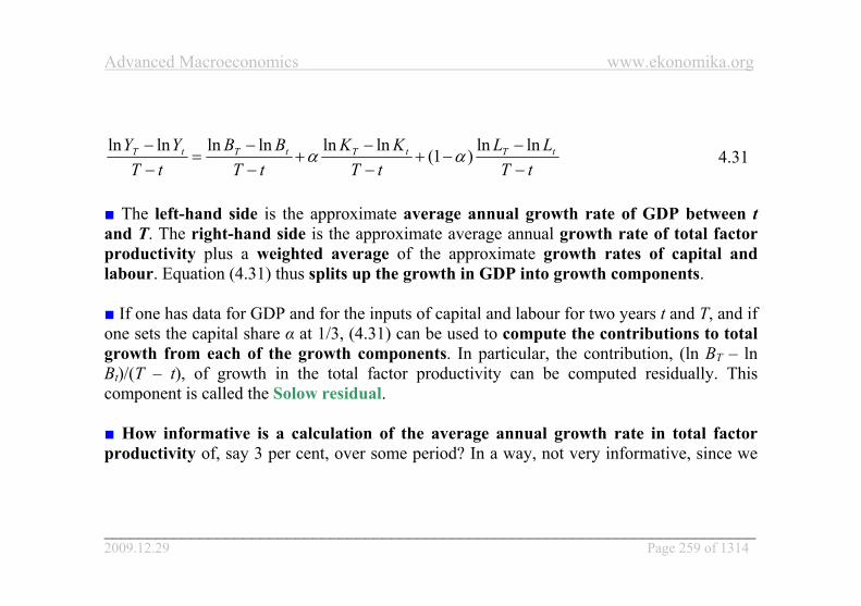
=−− lnln)1(lnlnlnlnlnln

αα 4.31

■ The left-hand side is the approximate average annual growth rate of GDP between t and T. The right-hand side is the approximate average annual growth rate of total factor productivity plus a weighted average of the approximate growth rates of capital and labour. Equation (4.31) thus splits up the growth in GDP into growth components. ■ If one has data for GDP and for the inputs of capital and labour for two years t and T, and if one sets the capital share α at 1/3, (4.31) can be used to compute the contributions to total growth from each of the growth components. In particular, the contribution, (ln BT – ln Bt)/(T – t), of growth in the total factor productivity can be computed residually. This component is called the Solow residual. ■ How informative is a calculation of the average annual growth rate in total factor productivity of, say 3 per cent, over some period? In a way, not very informative, since we


___________________________________________________________________________ 2009.12.29 Page 260 of 1314

do not really know what Bt is. We have simply put all factors of importance for aggregate production other than physical capital and labour into Bt. ■ Solow himself has expressed this by saying that the Solow residual may be viewed as “a measure of our ignorance”. However, although we do not know exactly what an increase in Bt represents, growth accounting exercises may be useful. ■ For instance, one could compare the Solow residuals between two different periods for one country, or between two different countries for the same period. If one residual is considerably larger than the other, the contribution to growth coming from unknown factors has changed from one period to the other, or has been larger in one country than in the other. Lower growth in Bt may be the first warning that productivity is not developing as favourably as it used to, or as favourably as in some other country. ■ One can also do growth accounting per worker. The production function (4.29) implies that yt = Btkt

α in the usual notation. Taking logs and time differences gives:


___________________________________________________________________________ 2009.12.29 Page 261 of 1314

tTkk

tTBB

tTyy tTtTtT

−−

+−−

=−− lnlnlnlnlnln

α 4.32

■ For Bt = At

1-α, this equation may be rewritten in terms of A, to give

tTkk

tTAA

tTyy tTtTtT

−−

+−−

−=−− lnlnlnln)1(lnln

αα 4.33

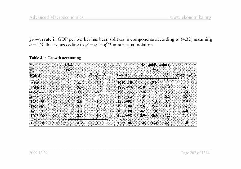
expressing the growth rate of yt as the weighted average of the growth rates of At, and kt. Equation (4.32) splits up the growth in GDP per worker into contributions from growth in capital per worker and growth in total factor productivity. Again, from data on GDP per worker and capital per worker, and setting α = 1/3, one can determine the growth contribution from technology (or other factors) residually. ■ Table 4.1 reports on a growth accounting exercise for six different countries. For each country and for five-year periods between 1960-1965 and 1995-2000, the average annual


___________________________________________________________________________ 2009.12.29 Page 262 of 1314

growth rate in GDP per worker has been split up in components according to (4.32) assuming α = 1/3, that is, according to gy = gB + gk/3 in our usual notation. Table 4.1: Growth accounting


___________________________________________________________________________ 2009.12.29 Page 263 of 1314


___________________________________________________________________________ 2009.12.29 Page 264 of 1314

Sources: OECD, Economic Outlook Database. ■ Consider first the figures for the US. As you will see, over the full period from 1960 to 2000, capital and GDP (per worker) grew at almost the same rate. This indicates that the US was close to balanced growth over the period (and so was Belgium, while for the other


___________________________________________________________________________ 2009.12.29 Page 265 of 1314

countries the capital-output ratio either decreased or increased substantially). In the first five-year period TFP (total factor productivity) growth in the US was 2.9 per cent per year, which is high. To illustrate, note that a gB of 2.9 per cent (per year) corresponds to gA of 4.4 per cent for α = 1/3 (from At = Bt

1/(1-α) it follows that gA = gB/(1 – α)), and under balanced growth, gA is directly comparable to gy. Annual growth rates in GDP per worker of around 4.4 per cent are very high and unusual as averages over longer periods in Western, early industrialized countries. ■ The period of high TFP growth in the US was followed by a considerable slowdown with quite low rates of TFP growth in the late 1960s and 1970s, followed again by a partial return to higher TFP growth in the 1980s and 1990s. The downward movement in TFP growth in the middle of the period has been called the “great productivity slowdown”, and you will see from Table 4.1 that the UK, Belgium, Sweden and Denmark experienced similar slowdowns, while Ireland seems to have been developing quickly throughout the period. Economists have searched for reasons for the international productivity slowdown described.


___________________________________________________________________________ 2009.12.29 Page 266 of 1314

■ We will not go into detail about the explanations offered. Some have suggested that the oil crises of 1973 and 1979 were responsible (but note that the slowdown in the US started before that). Others have stressed the relative shift in the production mix away from manufacturing towards the more labour intensive production of services where productivity gains may be harder to achieve. ■ Still others have claimed that declines in the quality of the labour force or of infrastructure caused the slowdown. Moreover, some have argued that it is not the low TFP growth of the 1970s and 1980s that need explanation. Rather it is the high TFP growth in the 1960s that is unusual and needs to be explained. ■ There are pros and cons for all these hypotheses. What we want to emphasize is that the evidence from a growth accounting exercise has induced people to think about what was going on. This illustrates that growth accounting is a useful tool for economic analysis. ■ Growth accounting only uses a production function and some knowledge of parameters (like α). The production function does not have to be as simple as (4.29) above. It is often


___________________________________________________________________________ 2009.12.29 Page 267 of 1314

argued that growth accounting should allow not only for the quantity of labour input, measured in hours or man-years, but also for the quality of labour input, measured by the average level of education. ■ It is natural to measure the average level of education in year t by the average number of years, ut, that people in the year t labour force have spent on education (in school, say). The quality of labour would then be given by an increasing function h(ut), often referred to as a human capital function, and the aggregate production function would be modified to:

Yt = BtKtα(h(ut)Lt)1-α 4.34

■ We cannot do growth accounting based on (4.34) until we know more about the function h(ut). Here some results from labour economics can be of use. Many labour economists have studied the relationship between education and wages. One of their findings (most often based on microeconomic data) is that a specific absolute change in the amount of education, one more year in school say, seems to give rise to a specific relative


___________________________________________________________________________ 2009.12.29 Page 268 of 1314

change in the wage rate. (A pioneering contribution is Jacob Mincer, Schooling, Experience, and Earnings, Columbia University Press, 1974.) By assuming the functional form: h(ut) = exp(ψut), ψ > 0, we obtain an increasing human capital function with exactly this property (just take logs on both sides and differentiate with respect to ut):

ψ=tt

t duuhudh /

)()(

■ That is, one additional year of education yields a certain relative increase (ψ) in the level of human capital independently of the initial ut. Let us now try to estimate ψ. If labour is paid its marginal product, then (4.34) implies that the wage rate, wt, should be:


___________________________________________________________________________ 2009.12.29 Page 269 of 1314

))1exp(()1()()1( 1t

t

ttttttt u

LKBLuhKBw ψααα

αααα −⎟⎟

⎠

⎞⎜⎜⎝

⎛−=−= −−

■ Taking logs on both sides and differentiating with respect to ut gives:

ψα )1(/ −=tt

t wdudw

■ Thus a one-year increase in schooling gives a relative increase in pay equal to (1 – α)ψ. A rather robust finding in empirical studies (mainly for the US, but for some other countries as well) is that the percentage increase in pay generated by a one-year increase in schooling is around 7 per cent. If (1 – α)ψ is roughly equal to 0.07, and α is 1/3, then ψ must be approximately 0.1 (10 per cent). With the production function: Yt = BtKt

α(exp(ψut)Lt)1-α 4.35


___________________________________________________________________________ 2009.12.29 Page 270 of 1314

and knowledge of the parameters α and ψ, we can do growth accounting again. In per worker terms the appropriate formula following from (4.35) is:

tTuu

tTkk

tTBB

tTyy tTtTtTtT

−−

−+−−

+−−

=−−

ψαα )1(lnlnlnlnlnln4.36

■ Note that it is not the average relative change in schooling from year t to T that enters the formula, but the average absolute change. From data on GDP per worker, capital per worker, and average years of schooling of the labour force in two different years t and T, one can again split up growth into the contributions from growth in capital per worker, growth in education, and the residual growth in TFP. ■ In particular, if a country has experienced a large increase in education over the period considered, one may tend to exaggerate the contribution from TFP growth if one does not include education in the growth accounting. This may be particularly relevant for an


___________________________________________________________________________ 2009.12.29 Page 271 of 1314

assessment of TFP growth in the growth miracle countries of East Asia. The East Asian tiger economies have typically experienced huge increases in educational effort. ■ If one ends up finding that a certain country has had considerably higher TFP growth than another, controlling appropriately for differences in education, one can go on looking for other neglected factors of production to explain the difference. ■ The tiger economies do indeed tend to exhibit very high TFP growth even after one has controlled for education. One explanation which has been suggested is that over the periods most often considered, the West has experienced a larger shift of the production mix from manufacturing to services than East Asia. It is an open question whether, taking all relevant factors into account, East Asia has had above-average TFP growth, or whether its high growth is simply due to above-average factor accumulation. ■ A growth accounting exercise can split up growth in GDP or in GDP per worker into components, thus attributing total growth to various sources. However, this does not identify the causes of the growth. Here is why. Assume that the growth process of some economy


___________________________________________________________________________ 2009.12.29 Page 272 of 1314

can be described fully by the steady state of the Solow model with appropriate parameter values. In that case there will be positive growth in GDP per worker if and only if g > 0. ■ In a causal sense, all growth in GDP per worker will then be rooted in the exogenous growth of the technological variable. On the other hand, if one conducts a growth accounting exercise, one will find that the growth in GDP per capita comes partly from technological growth and partly from growth in capital per worker. Both observations will be true. ■ Without technological growth there would be no growth in GDP per worker, so technological growth is the ultimate source of long-run growth. However, when there is (steady state) growth in GDP per worker (and hence in technology), there will also be growth in capital per worker, so part of the growth observed comes from capital accumulation. Summary


___________________________________________________________________________ 2009.12.29 Page 273 of 1314

■ In the basic Solow model the only source of long-run growth in economic activity is population growth. The basic Solow model cannot generate the long-run growth in GDP per capita that we observe in the data. ■ The general Solow model developed in this lecture generalizes the basic Solow model by introducing steady exogenous technological progress. This enables the model to generate long-run growth in GDP per capita. Technical progress may be labour-augmenting, increasing the efficiency of labour; it may be capital-augmenting, raising the productivity of capital, or it may take the form of an increase in total factor productivity. As long as the aggregate production function has the Cobb-Douglas form, all of these types of technological progress are equivalent and have the same implications for the evolution of the economy. ■ In the long run the general Solow model converges on a steady state with balanced economic growth, where total output, consumption, investment and the capital stock all grow at a rate equal to the sum of the exogenous growth rates of population and labour-augmenting productivity, where output per person, capital per person, consumption per person, and the real wage rate all grow at the same rate as labour-augmenting productivity, and where the real


___________________________________________________________________________ 2009.12.29 Page 274 of 1314

interest rate is constant. Hence the long-run economic predictions of the general Solow model accord with the basic stylized facts about long-run growth. Outside steady state the general Solow model accords with the observation of conditional convergence. ■ The general Solow model implies that structural economic policies which succeed in raising the economy's savings rate or in reducing its rate of population growth will gradually take the economy to a higher steady state growth path characterized by a higher level of steady state income and consumption. The general Solow model implies the same golden savings rule as the basic Solow model: long-run consumption per capita will be maximized when the savings rate equals the capital income share of GDP. ■ Structural policies which increase the savings rate or reduce the population growth rate cannot permanently raise the economy's growth rate. This can only be achieved via a policy that permanently raises the growth rate of factor productivity, but the general Solow model is silent about the factors determining technological progress.


___________________________________________________________________________ 2009.12.29 Page 275 of 1314

■ Empirical data for a large sample of countries around the world confirm the steady state prediction of the Solow model, that real GDP per worker will tend to be higher, the higher the investment rate and the lower the population growth rate. However, for reasonable values of the capital income share of GDP, the theoretical Solow model underestimates the observed quantitative effects of these structural characteristics. ■ Outside the steady state the general Solow model predicts conditional convergence: controlling for cross-country differences in structural characteristics, a country's growth rate will be higher, the lower its initial level of real GDP per worker. The data for countries around the world support this prediction, but for reasonable parameter values the theoretical model significantly overestimates the rate (speed) at which economies converge. ■ Using an aggregate production function, one can estimate the contributions to aggregate output growth stemming from increases in factor inputs and from increases in total factor productivity. Such a decomposition of the overall growth rate is called growth accounting. In basic growth accounting, growth in output per worker can originate from growth in the capital stock per worker or from growth in total factor productivity. Still, in a causal sense the


___________________________________________________________________________ 2009.12.29 Page 276 of 1314

ultimate source of growth is technological progress, since long-run growth in capital per worker can only occur if there is continued growth in total factor productivity.

4. technological progress and growth: … growth model. the general solow model ... figure 4.1: the...

Documents