ON SEPARATION PRINCIPLE FOR THE DISTRIBUTED ESTIMATION ANDCONTROL OF FORMATION FLYING SPACECRAFT

Amir Rahmani(1), Olivia Ching(2), and Luis A. Rodriguez(3)

(1)(2)(3)University of Miami, Coral Gables, FL 33146, a.rahmani@miami.edu

Abstract: This work presents a distributed estimation and control architecture for for-mation flying spacecraft. We show how spacecraft can individually create a local esti-mate of the formation and create their own control action using that estimate. Proofsare provided to show that such a scheme is asymptotically stable and spacecraft willreach consensus on the formation states.

Keywords: Distributed Formation Control, Distributed Kalman Filter, Formation Esti-mation, Separation Principle.

1. Introduction

Distributed space systems are expected to enable us to carryout space missionsperceived impossible under the current monolithic design. The distributed nature ofthese spacecraft allows us to launch missions that rely on coordination among smallerspacecraft, improving the overall system reliability. However, a number of technicalchallenges should be resolved before such systems can successfully function to theirmaximum potential, and as a coherent unit. A fundamental question is: How shouldthe control system for such a space system be designed?

Scharf et al. provided a comprehensive survey on guidance and control techniquesfor formation flying spacecraft [6, 7]. In general, one approach is to use a central-ized estimation and control scheme. While possible, this approach does not allow foreasy transition for changes in information exchange network or number of spacecraftin formation. Alternatively, in the distributed estimation and control architecture, eachspacecraft individually estimates its own and the formation states based on the infor-mation received from its neighbors. These estimated states are used to locally createthe control signal used for each spacecraft.

A large class of distributed estimator and controllers rely on information exchange net-works modeled as communication graphs. A survey by Garin and Schenato discussessome of the distributed control and estimation techniques based on the consensus al-gorithms on the interaction graphs [1]. Olfati-Saber has proposed a distributed KalmanFiltering scheme using consensus algorithm for a group of sensors that, collectively,estimate states of a process [4]. Olfati and Jalalkamali have extended these resultsto the case of mobile sensors who estimate the state of a moving target and in theprocess try to improve an information measure [5].

Rantzer focused on the case where several controllers with access to different mea-surements collectively control a system [9]. Smith and Hadaegh proposed a system ofparallel observers with noisy communication links and show under certain measure-ment and communication constraints, formation will be stable [8]. Hong et al. studieda leader follower network where followers have to estimate the velocity of the lead-ers [2]. Yang et al., on the other hand, considered estimating some formation statistics

1

(a) (b)

Figure 1: (a) Information exchange network in distributed spacecraft constitutes agraph (b) Proposed distributed estimation and control architecture.

as a measure for current shape of the formation and use these individually estimatedstatistics to locally generate controls which are applied to each agent [10].

The fundamental question is What is the best and most versatile distributed estimationand control scheme for such system and can one be designed independent of theother?

This work presents a distributed estimation and control architecture for formation flyingspacecraft where each spacecraft updates an estimate of its own as well as the forma-tion states based on its local observations and information received from its neighbors.In return these estimates are used to generate a local control that collectively will drivethe spacecraft to the desired formation.

2. Problem formulation

Consider n spacecraft with linear dynamics

xi(t) = Aixi(t) +Biui(t) + vi(t), (1)

where index i ∈ {1, . . . , n} and v is a zero mean Gaussian noise. Defining collectivevectors of state, control, and process noise respectively as x = col{x1, x2, . . . , xn},u = col{u1, u2, . . . , un}, and v = col{v1, v2, . . . , vn}. Process noise vector v is zeromean Gaussian with covariance Q. The collective dynamics of all spacecraft can berepresented as a linear system of the form

x(t) = Ax(t) +Bu(t) + v(t). (2)

The state and control matrices are diagonal matrices comprised of the individualspacecraft dynamic matrices, i.e. A = diag{A1, A2, . . . , An} and B = diag{B1, . . . , Bn}.

In a centralized control framework, one can design a stabilizing feedback controlleru(t) = Kx(t) that result in desired formation. This can be achieved through a variety

2

of techniques such as pole-placement and optimal control to name a few. Now, thechallenge is to implement such control strategy in a decentralized manner. This prob-lem can be divided into two parts: (i) Each spacecraft should be able to estimate thestates of the whole formation; (ii) Each spacecraft should compute and implement itsown control input only. Just like any monolithic system, the fundamental question iswhether the Separation Principle still holds for such design; i.e. does these individuallydesigned control and estimation subsystem work together to render the system stableand reach the goal of the control?

3. Distributed Estimation

Each Spacecraft is assumed to have sensors that can measure some of its own statesas well as that of potentially some neighboring spacecraft. Zero mean Gaussian mea-surement noise wi with covariance Ri is considered to corrupt the measurement, i.e.

zi = Hix+ wi. (3)

For the collective system of spacecraft described by (2) and individual spacecraft mea-surements (3); Provided that the pair (A,H) with H = [HT

1 HT2 . . . HT

n ]T is observablewe use the result of Olfati-Saber [4] to propose a distributed Kalman Filter with dynam-ics

˙xi = (A+BK)xi +Ki(zi −Hixi) + γPi

∑

j∈Ni

(xj − xi),

Ki = PiHTi R−1i , (4)

Pi = (A+BK)Pi + Pi(A+BK)T +Q−KiRiKTi .

Here xi represents the estimated estates of the whole formation by spacecraft i (not tobe mistaken by xi, which represents the states of spacecraft i and has a much smallersize), Ki is the optimal Kalman gain, and Pi represent the covariance of the estimationerror with dynamics presented in third equation of (4).

It is assumed that some spacecraft share their estimate of the formation states xi withother spacecraft through an information exchange network. This network can be rep-resented by a graph G(V , E). The vertex set V is the index of satellite in formation andedge set E is the set of unordered pairs (i, j) of indices of communicating spacecraft.Two spacecrafts are called neighbors1 if they share an edge, i.e. (i, j) ∈ E ⇔ j ∈ Ni.Figure 1(a) depicts how the information exchange network is presented as a graphwith spacecraft as nodes and communication links as edges.

The last term of first equation drives the estimation dynamics toward consensus on theestimated states xi. Its contribution depends on the sum of the difference between ownestimate and that received from its neighbors, as well as confidence in own estimate,represented by error covariance Pi, and a positive constant γ that selects how muchweight should be given to the consensus versus the local Kalman filter dynamics.

In this design it is sufficient that the collection of all spacecraft measurements H andstate matrix A be an observable pair. This condition is a much relaxed requirement,

1Not necessarily physical neighborhood, although in cases of limited power communication physicalneighbors are the same as ∆-disk graph neighbors.

3

compared to the proposed parallel observers of [8] which requires all pairs (A,Hi) tobe observable. Another advantage is that the current formulation use the knowledge ofnoise statistics and system dynamics to generate the provably most optimal estimateof the states.

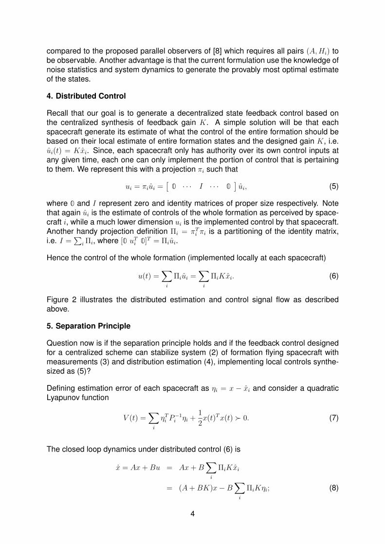
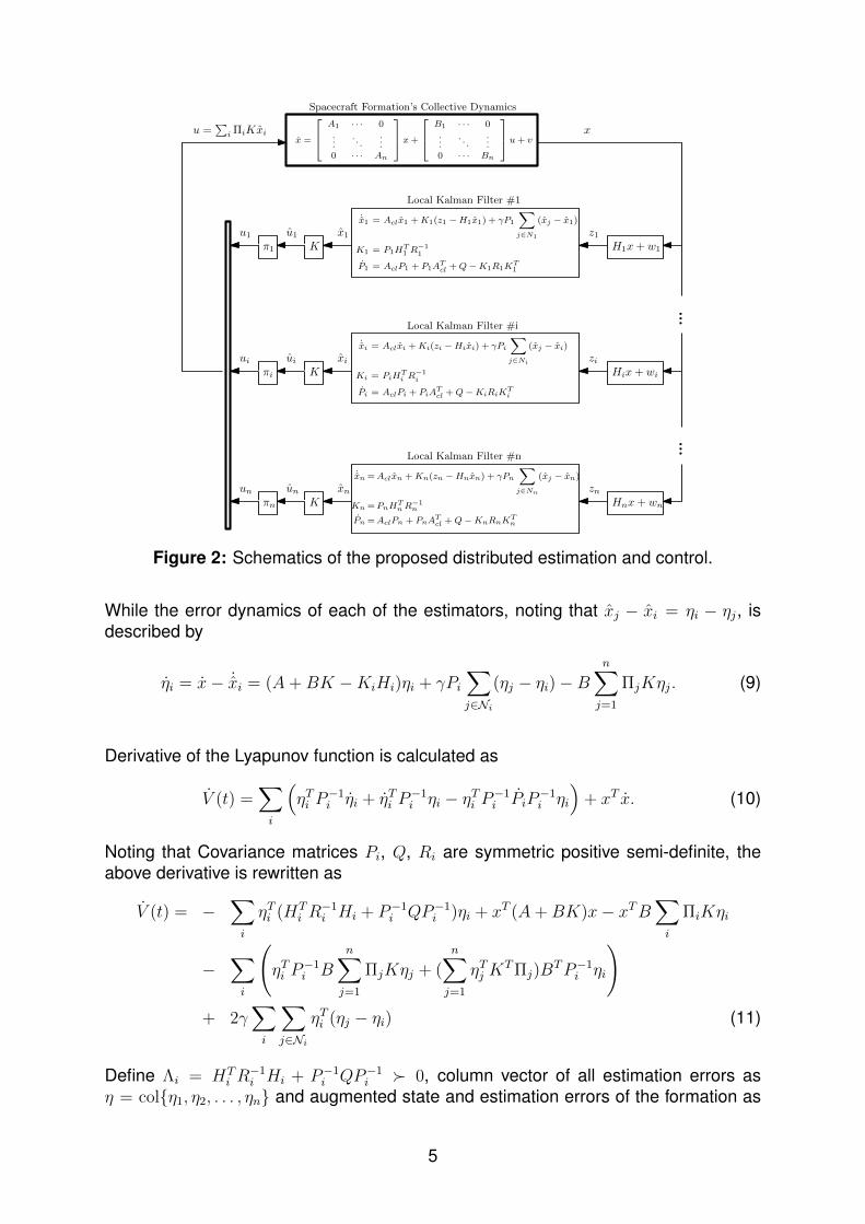
4. Distributed Control

Recall that our goal is to generate a decentralized state feedback control based onthe centralized synthesis of feedback gain K. A simple solution will be that eachspacecraft generate its estimate of what the control of the entire formation should bebased on their local estimate of entire formation states and the designed gain K, i.e.ui(t) = Kxi. Since, each spacecraft only has authority over its own control inputs atany given time, each one can only implement the portion of control that is pertainingto them. We represent this with a projection πi such that

ui = πiui =[

0 · · · I · · · 0]ui, (5)

where 0 and I represent zero and identity matrices of proper size respectively. Notethat again ui is the estimate of controls of the whole formation as perceived by space-craft i, while a much lower dimension ui is the implemented control by that spacecraft.Another handy projection definition Πi = πT

i πi is a partitioning of the identity matrix,i.e. I =

∑i Πi, where [0 uTi 0]T = Πiui.

Hence the control of the whole formation (implemented locally at each spacecraft)

u(t) =∑

i

Πiui =∑

i

ΠiKxi. (6)

Figure 2 illustrates the distributed estimation and control signal flow as describedabove.

5. Separation Principle

Question now is if the separation principle holds and if the feedback control designedfor a centralized scheme can stabilize system (2) of formation flying spacecraft withmeasurements (3) and distribution estimation (4), implementing local controls synthe-sized as (5)?

Defining estimation error of each spacecraft as ηi = x − xi and consider a quadraticLyapunov function

V (t) =∑

i

ηTi P−1i ηi +

1

2x(t)Tx(t) � 0. (7)

The closed loop dynamics under distributed control (6) is

x = Ax+Bu = Ax+B∑

i

ΠiKxi

= (A+BK)x−B∑

i

ΠiKηi; (8)

4

Local Kalman Filter #i

Hix+ wiKxiui zi

πi

ui

˙x1 = Aclx1 +K1(z1 −H1x1) + γP1

∑

j∈N1

(xj − x1)

K1 = P1HT1 R−11

P1 = AclP1 + P1ATcl +Q−K1R1K

T1

Local Kalman Filter #1

H1x+ w1Kx1u1 z1

π1

u1

Local Kalman Filter #n

Hnx+ wnKxnun zn

πn

un

x =

A1 · · · 0...

. . ....

0 · · · An

x+

B1 · · · 0...

. . ....

0 · · · Bn

u+ v

Spacecraft Formation’s Collective Dynamics

xu =∑

i ΠiKxi

...

...

˙xi = Aclxi +Ki(zi −Hixi) + γPi

∑

j∈Ni

(xj − xi)

Ki = PiHTi R−1i

Pi = AclPi + PiATcl +Q−KiRiK

Ti

˙xn =Aclxn +Kn(zn −Hnxn) + γPn

∑

j∈Nn

(xj − xn)

Kn =PnHTnR−1n

Pn =AclPn + PnATcl +Q−KnRnK

Tn

Figure 2: Schematics of the proposed distributed estimation and control.

While the error dynamics of each of the estimators, noting that xj − xi = ηi − ηj, isdescribed by

ηi = x− ˙xi = (A+BK −KiHi)ηi + γPi

∑

j∈Ni

(ηj − ηi)−Bn∑

j=1

ΠjKηj. (9)

Derivative of the Lyapunov function is calculated as

V (t) =∑

i

(ηTi P

−1i ηi + ηTi P

−1i ηi − ηTi P−1i PiP

−1i ηi

)+ xT x. (10)

Noting that Covariance matrices Pi, Q, Ri are symmetric positive semi-definite, theabove derivative is rewritten as

V (t) = −∑

i

ηTi (HTi R−1i Hi + P−1i QP−1i )ηi + xT (A+BK)x− xTB

∑

i

ΠiKηi

−∑

i

(ηTi P

−1i B

n∑

j=1

ΠjKηj + (n∑

j=1

ηTj KTΠj)B

TP−1i ηi

)

+ 2γ∑

i

∑

j∈Ni

ηTi (ηj − ηi) (11)

Define Λi = HTi R−1i Hi + P−1i QP−1i � 0, column vector of all estimation errors as

η = col{η1, η2, . . . , ηn} and augmented state and estimation errors of the formation as

5

η = [xTηT ]T , the above equation is transformed to

V = − ηT

−A−BKΛ1

. . .Λn

η − 2γηTLη

− ηT

0 BΠ1K BΠ2K · · · BΠnK0 P−11 BΠ1K P−11 BΠ2K · · · P−11 BΠnK0 P−12 BΠ1K P−12 BΠ2K · · · P−12 BΠnK...

......

...0 P−1n BΠ1K P−1n BΠ2K · · · P−1n BΠnK

η

− ηT

KTΠ1BTP−11 KTΠ1B

TP−12 · · · KTΠ1BTP−1n

KTΠ2BTP−11 KTΠ2B

TP−12 · · · KTΠ2BTP−1n

......

...KTΠnB

TP−11 KTΠnBTP−12 · · · KTΠnB

TP−1n

η. (12)

The first term in (12) is a diagonal matrix,M1, of positive definite matrices Λi � 0 andthe negative of closed loop state matrix. By design, control gain K is chosen such thatthe closed loop system is stable, i.e. A + BK ≺ 0. Hence the first term is positivedefinite. The second term is quadratic in L = L(G) ⊗ IN , where L(G) represent theLaplacian of the information exchange graph G and IN is identity matrix of the sizeN = |x|, size of vector x. As seen in [3], this matrix is positive semi-definite hencethis term also is positive semi-definite, i.e. −2γηTLη ≺ 0. The next step is to find theeigenvalues of the two remaining matrices to determine the stability of the synthesizedestimation and control scheme.

The first matrix can be reduces to a lower diagonal matrix using a similarity transfor-mation

S =

I −Pn

P1 −Pn

. . . ...Pn

and S−1 =

I IP−11 P−11

. . . ...P−1n

.

Similarly, a similarity transformation of the form

S =

P−11

P−12. . .

−P−11 −P−12 · · · P−1n

and S−1 =

P1

P2

. . .−Pn −Pn · · · Pn

,

is used to upper diagonalize the last matrix of equation (12). We choose to use thesematrices because eigenvalues of a matrix do not change under similarity transforma-tions.

6

Hence,

SM3S−1 =

0 0 0 · · · 00 0 0 · · · 00 0 0 · · · 0...

......

...0 BΠ1KP

−11 BΠ2KP

−12 · · ·

∑iBΠiKP

−1i

, (13)

and

SM4S−1 =

0 0 · · · P−11 KTΠ1BT

0 0 · · · P−12 KTΠ2BT

......

...0 0 · · ·

∑i P−1i KTΠiB

T

. (14)

Eigenvalues of these lower (upper) diagonal matrices are represented by the eigen-values of its diagonal blocks. Other than a number of zero eigenvalues these matriceshave similar eigenvalues (one is the transpose of the other) represented by eigen-values of the matrix

∑iBΠiKP

−1i . Consequently, a sufficient condition for the pro-

posed distributed control to be stable and for the separation principle to hold is that∑iBΠiKP

−1i be positive semi-definite. Matrices P−1i are symmetric positive definite

and∑

iBΠiK = BK. Under the above condition, derivative of the Lyapunov functionis negative definite and system is asymptotically stable. The estimation errors ηi willreach zero, i.e. xi = x (for more details see [3]).

It is noteworthy that the collective dynamics of all spacecraft states and their estimationerror from (8) and (9) is

˙η = (M1 +M2 +M3) η, (15)

where

M1 =

A+BKA+BK −K1H1

. . .A+BK −KnHn

,

M2 =

I...I

[

0 BKΠ1K · · · BKΠNK],

M3 =

[0

L(G)⊗ IN

].

The proposed Lyapunov function (7) is quadratic on η, which evolves based on theabove mentioned equation, i.e.

V (t) = ηT

12I

P−11. . .

P−1n

η.

7

6. Conclusions

We show that under certain conditions a feedback controller designed to stabilize aspacecraft formation can be used to generate control signals locally. Control inputsare generated locally using distributed estimation of full formation states based on localmeasurements and communication with some neighboring spacecraft. The conditionfor stability of the spacecraft formation calls for

∑iBΠiKP

−1i to be positive definite.

This is the direct result of using a Lyapunov stability analysis on a system comprised ofall spacecraft states and their estimation estates. Proper adjustments to the estimationfilters can potentially relax the stability condition provided and is the topic of our futurestudies.

References

[1] F. Garin and L. Schenato, “A Survey on Distributed Estimation and Control Appli-cations Using Linear Consensus Algorithms,” In A. Bemporad, M. Heemels, andM. Johansson (Ed.), Networked Control Systems, Springer, 2010.

[2] Y. Hong, G. Chen, and L. Bushnell, “Distributed Observer Design for Leader-Following Control of Multi-Agent Networks,” Automatica, Vol. 44, pp. 846–850,2008.

[3] R. Olfati-Saber and R.M. Murraysurv, “Consensus Problems in Networks ofAgents With Switching Topology and Time-Delays,” IEEE Transactions on Au-tomatic Control, Vol. 49, No. 9., Sep. 2004.

[4] R. Olfati-Saber, “Distributed Kalman Filtering for Sensor Networks,” IEEE Confer-ence on Decision & Control, New Orleans, LA, Dec. 2007.

[5] R. Olfati-Saber and P. Jalalkamali, “Coupled Distributed Estimation and Controlfor Mobile Sensor Networks,” IEEE Transactions on Automatic Control, Vol. 57,No. 9., Sep. 2012.

[6] D.P. Scharf, F.Y. Hadaegh, and S.R. Ploen, “A survey of spacecraft formationflying guidance and control (part 1): guidance,” American Control Conference,Denver, CO, 2003.

[7] D.P. Scharf, F.Y. Hadaegh, and S.R. Ploen, “A survey of spacecraft formation flyingguidance and control (part II): control,” American Control Conference, Boston,MA, 2004.

[8] R. Smith and F.Y. Hadaegh, “Colosed-Loop Dynamics of Cooperative Vehicle For-mations with Parallel Estimators and Communication,” IEEE Transactions on Au-tomatic Control, Vol. 52, No. 8., Aug. 2007.

[9] A. Rantzer, “A Separation Principle for Distributed Control,” IEEE Conference onDecision & Control, San Diego, CA, Dec. 2006.

[10] P. Yang, R.A. Freeman, K.M. Lynch, “Multi-Agent Coordination by DecentralizedEstimation and Control,” IEEE Transactions on Automatic Control, Vol. 53, No. 11,Dec. 2008.

8