4.3.2.1 methods and materials three coves representing the

4-9

4.3 Standing Crop Estimates

4.3.1 Introduction

Fish populations are generally assessed in terms of standing crop or

weight of fish per unit area. The examination of standing crop incorporates

the various factors affecting a fish populati6n and allows for comparison among

areas and bodies of water.

Standing crop estimations of fishes are commonly made by introducing

a toxicant in an 'area of known size and examining fish that are killed. This

method contains the inherent variability of changing physical and environmental

conditions and of varying efficiency of sampling. Cove "samples (the poisoning'

of coves isolated with block nets) have, however, been found to provide an esti

mate of fish biomass which is often better than other assessment methods, although

relative abundance may be misrepresented (Barry, 1967; Hayne et al.,1967; and

Sandow, 1970).

4.3.2.1 Methods and Materials

Three coves representing the upper, mid, and lower reaches of the

impoundment were selected for rotenone'sampling at Robinfon Impoundment during

1974 and 1975 (Figure 4.2.1). The coves were blocked off using 1/4-inch (delta) mesh

block nets. The surface area and volume-,of the coves were calculated

and Noxfish (5% emulsifible rotenone) applied at a concentration of 2.0 parts

per million. -Potassium permanganate was applied outside of the block nets to

neutralize rotenone diffusing out of the coves. Fish'%,iere collected inside

the block net-as they-appeared after rotenone application aid-oiinthe following

day. Fish were separated by species; length and weight were recorded.' When

numbers warranted, fish were assigned to length groups and group weights were

recorded (1974 - inch groups, 1975 - centimeter groups). Scales and gonads

4-10

were removed from fresh warmouth, bluegill, chain pickerel, and largemouth bass which were collected. Fishes which could not be positively identified in the field were preserved in 10% formalin and returned to the laboratory

for further examination.

4.3.3 Results and Discussion

Standing crop estimates ranged from 29.3 kg/ha in the upper impoundment cove during 1975 to a high of 139.8 kg/ha in the lower impoundment cove during 1975 (Table 4.3.1). The greatest numbers of fishes in both 1974 and 1975 were found at the mid-impoundment transect; however, diversity was lower than at the other sampling locations. During both years, diversity was highest in the upper impoundment cove although no species were conspicuous by their presence or absence at any particular sampling location.

In the lower impoundment cove, chain pickerel, spotted suckers, bluespotted sunfish, and bluegills were, the major species collected during both years. The weight of redbreast sunfish collected decreased from 1974 to 1975 while the-weight of warmouth and largemouth bass increased considerably. Swamp darters were second in numerical abundance in the lower impoundment cove

during 1975.

The mid-impoundment cove was numerically dominated by bluegills during 1974 and 1975. The mean length of these fish was 33 mm and 71 mm during 1974 and 1975, respectively. Due to the length classes used, the 1974 lengths probably underrepresented the true mean. Generally, however, most bluegill were in the 2-3 inch size range. This small size indicates the abundance of young bluegills in the area. Other young centrarchids were also present in substantial numbers as evidenced by the numbers and average sizes of bluespotted sunfish of 26 and 50 mm and largemouth bass of 129 and 94 mm. The major fish species collected from the mid-impoundment cove in terms of biomass-were redfin and chain pickerel, bluegill, warmouth, and largemouth bass., The swampfish collected from the mid-impoundment cove should be noted since this little known species was not collected from any other locations during our sampling program.

'Data records used in calculating mean lengths were midpoints of length classes in cases where length classes were utilized in reporting lengths.

N'

4-11

The upper impounidment cove contained the greatest diversity of fishes although the standing crop was the lowest of the three coves sampled each year. Centrarchids, particularly bluespotted sunfish, warmouth, bluegill, and dollar sunfish were the major species collected comprising 85% and 76% of the total during 1974 and 1975. Numbers generally decreased from 1974 to 1975 (particularly bluegill) although the number of pickerel, pirate perch, and black banded sunfish increased. During both years of sampling, chain pickerel were major contributors to the total biomass. During 1974 spotted suckers-and during 1975 largemouth bass weights also were important.

During sampling in 1974, biologists present felt that several-factors contributed to underestimation of the fish populations in the mid-impoundment and lower impoundment coves. During the sample period, a wind blowing across the impoundment increased suspended material in the water and decreased visibility, causing a reduction in efficiency of collection. This wind also washed many small dead fish into the vegetation along the edges where recovery was impaired. In the lower impoundment cove, some difficulty was encountered in adequately fixing the block net from bottom to surface. This may have allowed the escape of some fishes and contributed to an underestimate of the-population.

The mean of the six rotenone samples collected from Robinson Impoundment during 1974 and 1975 were calculated and compared to other similar-lakes in the southeast (Table 4.3.2). Singletary, Alligator, Great,-and Catfish Lakes are characterized by low pH and black water. Lake Waccamaw has darkly stained water; however, pH is more nearly neutral and Par Pond, located on the Savannah River Reservation (ERDA), receives heated effluent.

Major species were considered individually in Table 4.3.2 witfother fishes combined and reported as "all others." When comparing Robinson Impoundment to the other lakes included, the standing crop estimate was somewhat less than Par Pond but greater than the others. Species composition and general abundance of fishes was similar in the lakes examined with bluegill, warmouth, chain pickerel, and largemouth bass frequently occurring as dominant species.

The standing crop data collected from Robinson Impoundment illustrated several points.

4-12

1. The standing crop of fishes is similar to other coastal plain

lakes in the Southeast.

2. Relative abundance of fish species as estimated with rotenone

is similar in Robinson Impoundment and other lakes in the South

east which have similar environmental characteristics.

3. Fishes are utilizing upper, mid, and lower reaches of Robinson

Impoundment, although abundance and diversity varies among areas.

4. Although surface temperatures in some areas of Robinson Impoundment

approach thermal maxima for many of the species collected, fish are present in good numbers, possibly indicating the utilization of

temperature stratified or refuge areas. There are many springs,

seeps, and small creeks in the area which are sources of rela

tively cool water. This cool water forms a layer close to the bottom which varies in size with volume of source water, turbu

lence, and bottom topography. Many of these areas are too small

to be illustrated from temperature/D.O. profile sampling, but are

readily apparent when wading in the area. In addition, much of

the impoundment has some temperature variation from top to bottom

(temperature - profiles, Section 3) providing large volumes of

water with temperatures less than those apparent on the surface.

5. No paucity of game or sport fish expected in a southeastern lake

or reservoir with similar environmental characteristics was

indicated by the rotenone samples collected from any area of

Robinson Impoundment.

4.4 Food Habits

4.4.1 Introduction

Fish food habits can provide valuable information on the patterns of energy flow within a community and indicate relationships potentially subject

to adverse environmental impact. These data can be useful in the interpretation

4-13

of fish growth rates, distributions, and reproductive efforts. The objectives

of the study program were: (1) to procure information on the types and relative

abundances of food items; (2) to qualitatively identify the major pathways and

sources of energy available for fish production; and (3) to qualitatively assess

the feeding conditions of the populations in question by comparison of seasonal

diets with the availability of resource items in the environment.

4.4.2 Methods and Materials

Species of important sport fishes selected for stomach analysis at

Robinson Impoundment included the bluegill, largemouth bass, warmouth, and

chain pickerel! A preliminary study of the bluegill was conducted from April

to December of 1974 from specimens collected from the intake screens of the

H. B. Robinson Steam Electric Plant. In January of 1975 a more intensive

sampling program was initiated to provide information on the food habits of

fishes from the upper, discharge and lower portions of the impoundment. Fishes

were collected monthly in the littoral areas of transects A, E, and G by use of

a Smith-Root Type VI boat mounted electrofisher and assorted other sampling

methods. Electrofishing in the vicinity of each transect from January to

December accounted for 82% of the yearly sample. The remaining 18% of the

samples were obtained from seine, rotenone, gill net, and impingement samples.

Fishes were injected in the field with 40% formaldehyde solution and preserved

in 10% formalin for future analysis.

Laboratory analysis involved the measurement of total length (TL) to

the nearest millimeter and excision of the stomach from the pyioric sphincter

to the esophagus. Stomachs Were emptied of contents and stored in individual

vials of 70% ethyl alcohol with Rose Bengal biological stain. Contents were

later identified to the lowest taxonomic level practical by use of Pennak (1953),

Brooks and Kelton (i967), Parrish (1968), Johannsen (1969), and Deevey and Deevey

(1971). Only stomachs with identifiable food organisms were utilized in this

study. Food organisms were enumerated by taxa and if more than one item was

present in a stomach, the percentage of these items was determined by centrifu

gation in a Wintrobe tube, water displacement, or visual inspection. The percent

frequency of occurrence; mean number of organisms per stomach with food, and

either the percent average volume or the percent total volume of food items were

'White catfish were also included at the initiation of the study but numbers collected were insufficient for analysis.

4-14

calculated for all fish on a quarterly basis. The percent average volume is influenced by the frequency of 6 ccurrence of a kind of food but not by the size of either the stomach nor its fullness. This gives the stomach contents of small fish the same importance as those of a large fish and is applicable in describing volumetrically the food of bluegill. The percent total volume emphasizes the importance of large items and is applicable to the diets of large predaceous fish (i.e., warmouth, largemouth bass, chain pickerel). Bluegills from the lower impoundment and discharge area were divided into two groups (< 100 mm and > 100 mm TL) (< 3.9 in and > 3.9 in) in order to demonstrate any size differences in food selectivity. This was not possible in the upper impoundment due to small sample sizes.


Bluegill-Limnetic Zone of Lower Impoundment

Food analysis of bluegills from the intake screens of the H. B. Robinson Steam Electric Plant during 1974 is based on the examination of 168 stomachs (Table 4.4.1). These data (Figures 4.4.1 and 4.4.2) illustrate a dominance of zooplankton in the diet ýnd suggest a seasonal progression in numerical abundance and relative importance of zooplankton as food items. The dominant food item in the diet of small bluegill during the summer was Cyclops while Eubosmina was dominant during the fall. A comparison of food habits data with zooplankton dominance suggests that bluegills grazed upon the dominant forms available. Eubosmina was the winter and fall dominant while Cyclops was dominant during the spring and summer. During the summer Chaoborus constituted a large portion of the'total volume and occurred at greater frequencies in stomachs of large bluegill thanin small bluegill. During the spring Chaoborus was the dominant resource for both size groups of bluegill (Figures 4.4.1 and 4.4.2). No data were available on the numerical abundances and seasonal distributions of the pelagic instars of Chaob6rus.

Bluegills for stomach analysis'largely consisted of fish impinged from dusk to dawn of the following daý. In stomachs containing Chaoborus, 70% contained zooplankton (i.e., Cyclops, Eubosmina, and Diaphanosoma), 21% contained only Chaoborus, and only seven percent contained Chaoborus and benthic organisms. All

4-15

instars of Chaoborus are known to feed on cladocerans and copepods in the epilim

nion at night (Juday, 1921; McLaren, 1963). Two main periods of feeding have been

described for bluegills. The major period occurs in the late afternoon and the

other a few hours after dusk (Keast and Welsh, 1965). This would correspond to

the time when Chaoborus has vertically migrated into the 'water column to prey upon

zooplankton. Chaoborus generally escapes fish predation'during the day by retrea

ting to the hypolimnion (Juday, 1921; Stahl, 1966; Pope et al. 1973).

Benthic macroinvertebrates, represented by a total of 16 genera (Table

4.4.2), contributed little to the total volume of food of limnetic bluegills. The

dominant benthic organisms consumed'were dipterah larvae (11 genera)'and trichop

terans (3 genera). The larvae of Procladius were present at frequencies higher

than 10% in both size groups of fish throughout the year. This chironomid repre

sented between 2.7% and 5.3% of the total stomach volume of large bluegill and

between 2.2% and 7.2% of small bluegill.1 Trichopterans (i.e., Oecetis and

Polycentropus) were important benthic resources during the spring (Figures 4.4.1

and 4.4.2).

The primary sources of food for the bluegill in the area of the plant

intake structures were Chaoborus,'Eubosmina, Cyclops, and Qecetis. These data

depict the food of limnetic bluegill during their feeding period-in the evening

and stress the role of zooplankton in the diet. It has been"reprted that all

sizes of bluegill participate in'diel littoral-limnetic migrations but that as

fish length increases a reduction in the frequency of migration occurs. Bauman

and Kitchell (1974) suggested that it is energetically'advantageous for larger

fish not to migrate but to remain in the littoral zone. Since the littoral zone

habitat available for bluegill' grazing was limited in this'area of the impound

ment due to impoundment topography and bluegill densities were high,the .. dvan

tages of littoral feeding may be lost due to high competitive interactions for

a limited food supply. The best feeding 9trategy under thesi'conditions would

be for increased planktivory. This is what has been observed 'at Robijisonr

Impoundment for both size classes of bluegills.

Bluegill-Littoral Zone of Lower Impotndment'

Data for bluegills in the lower impoundment during 1975 are based on

the examination of 302 stomachs (Table 4.4.1) and indicate a major dependence

4-16

upon planktonic cladocerans and copepods during the winter, spring, and fall. Larger bluegills did not consume as large a portion of zooplankton as did smaller fish. This is typical of bluegill feeding behavior (Carlander, 1972). In small bluegills, Eubosmina accounted for 99.4% of the volume and occurred in 100% of the samples during the winter quarter (Figure 4.4.3). The dominant taxa of zooplankton throughout the year were Eubosmina, Diaphanosoma, and Cyclops. The dominant organism in the winter was Eubosmina, with Diaphanosoma dominant during the spring and summer, and Cyclops present in highest densities during the fall of 1975 (Figures 4.4.3 and 4.4.4). An examination of stomach content data with respect to zooplankton seasonal abundances indicates similar patterns of dominance (Table 5.3.4). Since bluegills are reported to be keenly responsive to search and capture time during grazing (Werner and Hall, 1974), it is energetically favorable for these fish to consume the dominant species available in the absence of any size selective feeding behavior (Canfer and

Blades, 1975).

In the lower impoundment benthic organisms, represented by 29 taxa (Table 4.4.2), were important components of the diets of both size groups of bluegill. These organisms volumetrically represented 30.8% and 46.8% of the diets of small and large bluegills during 1975. An increased utilization of benthic organisms with increasing fish length is a common feeding behavior of bluegills (Carlander, 1972). Literature references to the food habits of the bluegill from a wide variety of habitats indicate that zooplankton and aquatic insects are the dominant food items (Calhoun, 1966; Carlander, 1972). Young bluegill feed on small crustacea and aquatic insects while the adults prefer the larger aquatic insects, small crayfish and fish (Carlander, 1972). In general, an inverse relationship exists between body size and the percentage of zooplankton in the diet (Turner, 1955). Bluegills generally remain within the same trophic level throughout life but shift from plankton grazing to benthos feeding as size increases (Gerking, 1962).

The most commonly consumed benthic organisms were larval chironomids. Small bluegills utilized 17 genera of chironomids while 14 genera were present in the diet of large bluegill. Chironomids were most abundant during the spring but were noticeably reduced during the winter. Procladius was present in the

I-

4-17 -•

food of both size groups of bluegills throughout the year. Larger bluegills also consumed Polypedilum throughout 1975 in addition to Procladius. Procladius is generally found in the sub-littoral and profundal areas of Robinson Impoundment while Polypedilum is typically found in the littoral zone. Another littoral zone chironomid, Ablabesmyia, was an important food resource for both size groups (Figures 4.4.3 and 4.4.4). Chironomid and culicid pupae were important food items of large bluegills at most times of the year. Utilization of pupae was highest during the spring, occurring in 59.2% of the stomachs and representing 19.5% of the volume (Figure 4.4.4). Oecetis, usually a littoral trichopteran on sandy, or clay substrates, was a subdominant food item of small bluegills during the fall and occurred in 15.2% of the stomachs (Figure 4.4.3). During the summer large bluegills utilized Chaoborus-and terrestrial Myrinicinae as food resources. These collectively averaged 86.5% of the total volume (Figures 4.4.3 "and 4.4.4). The major sources of food for bluegills in the lower impoundment were Eubosmina, Diaphanosoma, Cyclops, Chaoborus, Polypedilum, Ablabesmyia, Oecetis, and dipteran pupae (Figures 4.4.3 and 4.4.4). Analysis of the dath with respect to z ooplankton (Section 5.0) and benthic data (Section 6.0) suggests that the dominant items in the diet were also dominant in the impoundment. These data indicate an overall major reliance on zooplankton as the major food resource in the lower impoundment. As indicated previously, dependence upon zooplankton was-probably a function of

habitat.

Bluegill-Discharge Area

In the discharge area zooplankton was-an important component'of the diet of both size:groups of bluegills during thewinter, spring, and summer as determined from analysis of 208 stomachs (Table 4.4.1). Eubosmina was the dominant food for all bluegills during the winter and summer (Figures 4.4.5 and 4.4.6) while Cyclops wasdominant during the spring (Figure 4.4.5). A'comparison' of zooplankton species composition in the discharge area (Table '5.3.4) with'food

habits data indicates selection for nondominant species.-'During the summer the dominant taxa in the plankton were Cyclops and Diaphanos6ma!(Table 5.3.4). Examination of-fish food habits indicate a high utilization of Eubosmina 'ranging from 27 to 35% of the volume (Figures 4.4.5 andZ4.4.6). •Zooplankton were almost eliminated in the area of the discharge during mid-summer (e.g., August) (Table 5.3.4). Fish utilized nondominant zooplankton species occurring occasionally

4-18

at relatively low densities.

Benthic organisms averaged 58.9% and 57.5% of the yearly food volume

of small and large bluegills, respectively. This utilization is higher in

comparison with utilization in the lower impoundment. The lower impoundment

is deeper with limited littoral areas while the discharge area has large

littoral areas available for bluegill grazing. In contrast' with the lower

impoundment, Procladius was not utilized to any great extent in the discharge

area. This area is shallow and not a preferred habitat for Procladius.

Procladius (aberrant), which were most abundant in the littoral areas of

Station E-1 (Table 6.3.3), were not utilized by bluegillslas a food resource.

The important chironomid in the diet was Polypedilum which was present through

out the year. It was the dominant food item of large bluegill during the spring

quarter in terms of both volume and frequency of occurrence (Figures 4.4.6).

Benthic data indicate that the numbers of Polypedilum were reduced in the area

of the discharge (Figure 6.3.2).- Ablabesmyia was an important food of small

bluegills during the summer in-the discharge area occurring in 29% of the

stomachs and representing 12% of the total volume (Figure 4.4.5). This chiro

nomid was present in the littoral areas of the discharge area and was not

affected by the thermal effluent (Section 6). Chaoborus larvae were utilized

throughout the year by large bluegills and during the spring, summer, and fall

by small bluegills. This organism was the dominant food of small bluegills

during the fall and one of the dominant resources of the larger bluegills

during both summer and fall (Figures 4.4.5 and 4.4.6). As indicated in the

benthos data, Chaoborus densities~were reduced in the discharge area during

the summer (Figure 6.3.4). As suggested in Section 6, this reduction in numbers

of Chaoborus resulted from elevatediwater temperatures and current velocities

associated with plant operations. Oecetis occurred in 36.7% of the large blue

gills and 50% of the small bluegills during the fall of 1975. This organism

was collected in relatively highnumbers at Transect E throughout 1975 (Figure

6.3.8). The food preferences of bluegills indicate utilization of several

items affected by the thermal effluent of Robinson Steam Electric Plant.

Diversity (d) estimates of benthic organisms were extremely low in the discharge

area during the summer (Table 6.3.7). Diversity was low at Station E-1 from

August to October of 1975 and a zero diversity was calculated-for the benthic

community during September and October. Diversity was also low at Station E-3

4-19

from July to October of 1975 (Table 6.3.7). According to Headrich (1975),

changes in community stability due to environmental changes are reflected by

changes in diversity.

The primary sources of food for bluegills in the discharge area were

Eubosmina, Chaoborus, Cyclops, Diaphanosoma, Ablabesmyia, Polypedilum, Oecetis,

Oligochaetes, and chironomid pupae and emergents. As indicated by the abundance,

species composition, and diversity of the benthos, the quality of feeding condi

tions in the discharge area during the summer was the poorest encountered in the

impoundment. During the summer,benthic organisms totaled 51% and 67% volume

trically of the food of small and large bluegill yet species diversity and

relative abundances of benthos in the habitatwere low. This lack of stability

of dominant food items in the discharge area suggests that a food stress exists

on those bluegills inhabiting this area. It has been suggested that bluegills

are overcrowded in Robinson Impoundment. Overcrowding is common in bluegill

populations and is one of the persistent problems of fisheries management. It

is not unusual for overcrowded populations to occur in marginal habitats. In

terms of available food supply, the discharge area must be considered a marginal

habitat during the summer months and that bluegills inhabiting this area were

food stressed.

Bluegill-Littoral Zone Upper Impoundment

The food habits of bluegills in the upper impoundment during 1975 as

based on the analysis of 114 fish (Table 4.4.1) were essentially different from

those of the lower and middle regions. -This was indicated by a greater dominance

diversity of food items (Figure 4.4.7), a greater number of different taxa

(Table 4.4.2),,and the presence of 19 taxa of benthos notpresent in the diet

of fish in the lower impoundment and discharge area. In the upper impoundment

rooted aquatic macrophytes were more abundant than in-other areas of the impound

ment (Figures 7.2.1, 7.2.2, 7.2.3, 7.2.4) and provided suitable habitat for many

macroinvertebrates. Of noticeable importance in the diet of bluegills in the

upper impoundment was a high percentage of large-bodied benthic organisms

(Figure 4.4.7). -In the lower impoundment Oecetisand Oxyethira were the only

trichopterans utilized by bluegills while in the upper impoundment at least

six different taxa were present in the diet (i.e., Agrypnia, Leptocella, Oecetis,

4-20

Oxyethira, Pharyganea, and Pycnopsyche). During the winter Pycnopsyche was one

of the major components of thepdiet (Figure 4.4.7). The major macroinvertebrate

utilized by bluegills throughout the year was Hexagenia (Figure 4.4.7). These

mayfly nymphs represented more than 20% of the volume during the winter, spring,

and fall. These organisms are noticeably absent in the lower and discharge areas

of the impoundment (Section 6). In the upper impoundment four dipteran larvae

(i.e., Ablabesmyia, Dicrotendipes, Polypedilum, and Pseudochironomus) were present

in the diet throughout the year.- This is in contrast with other areas of the

impoundment where Polypedilum and/or Procladius were present.

Zooplankton were not a dominant food resource for bluegill in the upper

impoundment except during the fall. Eubosmina was utilized to a great extent

during the fall quarter. It occurred in 73.3% of the stomachs and totaled 70.4%

of the volume (Figure 4.4.7). These organisms were extremely abundant in the

upper impoundment at this time (Table 5.3.4). In the lower and mid portions of

the impoundment when zooplankton were utilized to this extent, the number of

other taxa in the diet was generally reduced indicating primarily planktivorous

feeding behavior. This pattern was not observable in the upper impoundment. This

indicates greater stability in the diet. The food habits described for the blue

gill in the upper impoundment are typical of those found in the literature

(Carlander, 1972).

Largemouth Bass

Food habits of 24 fingerling bass (32-94 mm TL) during the spring and

summer at Robinson Impoundment indicate the importance of cladocerans and large

bodied invertebrates in the diet (Table 4.4.3). Kramer and Smith (1960) reported

that bass 40-100 mmTL fed on cladocerans, chironomid larvae, and ephemeropteran

nymphs. This feeding'pattern has also been well documented in other studies

(Carlander, 1972). At'Lake George, Minnesota, fish first appeared in the diet

when bass attained a total length of 20 mm but occurred in no more than 50% of

the stomachs (Kramer'and Smith, 1960). Murphy (1949) found that bass greater

than 71 mmTL fed almost exclusively on fish while Turner and Kraatz (1920)

stated that insects and fish were the principle foods of bass > 50 mmTL. At

Robinson Impoundment-fish occurred-in 54.6% of the stomachs during the spring

and 31.3% in the summer. Murphy (1949) concluded that high production of

4-21

young bass can be attained only if an ample supply of forage fish is avail

able when the fingerlings reach 63-75 mm total length. Appelgate and Mullan

(1967) attributed high bass production to the consumption of midge larvae

and cladocerans. The dominant forage fish for fingerling bass-was larval

and post-larval centrarchids which were most abundant in the upper impound

ment (Table 4.7.2) and should have provided an ample food supply for the

early stages of bass growth.

The major food items of adult largemouth bass (> 100 mmTL) at

Robinson Impoundment were fishes, crayfish, and odonate nymphs (Figure 4.4.8).

This was determined from the analysis of 51 stomachs (Table 4.4.1). Crayfish

and odonate nymphs are usually associated with rooted aquatic vegetation.

There are no estimates available from Robinson Impoundment on the distributions

or abundances of crayfish and odonates. Fishes represented by Lepomis,

Etheostoma, Notropis, and Micropterus were the dominant food items volumetri

cally during the winter (90.8%), spring (43.3%), summer (83.1%), and fall

(26.2%) of 1975 (Figure 4.4.8). During the fall, crayfish (Procambarus)

contributed 20.1% to the total volume and occurred in 35.7% of the stomachs.

The food habits of largemouth bass at Robinson Impoundment were typical of

literature descriptions of the diet in other lakes. The principle foods of

largemouth bass in other studies were small centrarchids, centrarchids and

crayfish, perch, crayfish and fish, gizzard shad and crayfish, gizzard shad

and crappies, gizzard shad and yellow bass, and fish in general (Goodson,

1965; Carlander, 1972). Odonates and mayfly numphs were the major groups

of insects consumed by large bass in Ontario (Carlander, 1972).

At RobinsonImpoundment the major.sources of food for fingerling

bass were hemipterans, chironomid pupae, Chaoborus, Palaemonetes, Lepomis,

and Etheostoma. Adult bass foraged to a great extent on fishes, particularly

Etheostoma, Lepomis, Micropterus, and Notropis. The dominant forage fish

throughout the year for all sizes of largemouth bass was Lepomis. Small

centrarchids, particularly bluegill, were abundant during most times of the

year at Robinson Impoundment and provided ample forage for largemouth bass.

"4-22

Warmouth

Food habits of warmouth from Robinson Impoundment as determined

from the analysis of 65 stomachs (Table 4.4.1), illustrated little seasonal

variation in food preference. The major food items were trichopterans,

ephemeropterans, odonates, crayfish, and fish (Figure 4.4.9). Warmouth are

generally found in areas of dense aquatic vegetation and soft bottoms

(Larimore, 1957). Crayfish are also inhabitants of this littoral zone

habitat and juveniles typically move about on the bottom during the daylight

in search of food. These crayfish are susceptible to fish predation and

were utilized as a food resource throughout the year. Crayfish were the

dominant food items during the spring, summer, and fall. Since crayfish

are detrital feeders, the primary sources of energy for warmouth growth was

derived from a detrital based food chain. Fish accounted for 21.5% of the

volume in the spring and 20.0% in the fall. Lepomis spp. were the dominant

forage fish consumed during 1975. Small bodied aquatic invertebrates and

zooplankton were consumed throughout the year to some extent but contributed

very little to the overall diet.

Small warmouth generally consume crustaceans and small invertebrates

while larger fish prey heavily upon crayfish and fish (Forbes, 1903; Lewis

and English, 1949; Larimore, 1957; German et al., 1973). Larimore (1957)

states based on his studies and a review of the literature that, "it

seems very unlikely that .there is any strong diet or highly restrictive food

preferences for this species." As indicated by the data from Robinson

Impoundment, warmouth principally consume crayfish and fish. This is

typical of what has been reported in the literature.

Chain Pickerel

Chain pickerel at Robinson Impoundment are largely piscivorous in

feeding behavior. Fish were the dominant items by volume during the winter

(73.5%), spring (99.8%), summer (93.1%) and fall (95.8%) of 1975 (Figure 4.4.10).

I

4-23

This was determined by the analysis of 67 pickerel stomachs (Table 4.4.1).

Forage species included Etheostoma, Lepomis, Erimyzon, Notemigonus, and

Fundulus. Foote and Blake (1945) found that fish represented over 90% of

the volume and occurred in 62% of ,the stomachs of pickerel from Babcock

Pond. Raney (1942) found that fishes totaled 47% of the volume -and that

species were not consumed in relation to their abundance in the pond.

In stomachs examined from Robinson Impoundment 82% had only one food item.

This characteristic of the feeding behavior of pickerel has been reported

by Raney (1942). In general, large pickerel feed mostly on fish, frogs,

crayfish, or almost anything of proper size (Calander, 1969). Food was not a

limiting factor for chain pickerel in Robinson Impoundment.

4.4.4 Summary and Conclusions

Planktivorous feeding was a dominant strategy of bluegills in the

lower and discharge areas of the impoundment. This is not an energetically

favorable feeding strategy of littoral bluegills especially for larger fish

(Bauman and Kitchell, 1974). Since the efficiency of protein utilization

decreases as fish become larger it is advantageous for larger bluegill to

feed on large-bodied benthic invertebrates in order to maximize the net

amount of energy available for growth (Gerking, 1962). This feeding strategy

was characteristic of bluegills in the upper impoundment. In this area of the

impoundment food habits of bluegill were typical of those described in the

literature and there was no evidence of food stress from either low produc

tivity or heat load. In the lower impoundment, which has limited littoral

areas available for bluegill grazing, the advantages of littoral feeding were

probably lost due to competitive interactions. In this area the most

energetically efficient feeding strategy was planktivory. In the discharge

area the quality of feeding conditions during the summer was the poorest

in the impoundment. Several dominant benthic food items were detrimentally

effected by plant effluents. During the summer benthos abundances and species

diversity were very low in the discharge area creating an unstable food

supply. This lack of stability of dominant food items in the discharge area

during the summer of 1975 indicated a food stress on the bluegill population.

This stress occurred on overcrowed bluegills in a marginal habitat with

limited and unstable food resources.

4-24

Food habits of largemouth bass, warmouth, and chain pickerel were

similar to literature descriptions and a comparison of food selectivity with

availability in the habitat suggest that food was not a limiting factor

for growth and reproduction. It should be pointed out, however, that these

studies were only descriptive and that no measurements were made of any

consumption rates or growth efficiencies. The dominant forage fish for

largemouth bass and warmouth was Lepomis spp. These centrarchids were abun

dant during most times of the year in the impoundment and should have provided

ample forage. Chain pickerel were found to be largely piscivorous.

Important forage species included Etheostoma, Lepomis, Erimyzon, Notemigonus,

and Fundulus. These species are widely distributed and common in Robinson

Impoundment and should have provided an ample food supply for chain pickerel.

The primary source of energy for the warmouth in the impoundment was detrital

based. This was indicated by the high rate of consumption of detrital

feeding crayfish. No estimates were available on the distributions and

abundances of crayfish in the impoundment, therefore, no conclusions can be

reached on the stability of a diet based on this dominant food resource.

4.5 Age and Growth Studies of Robinson Impoundment Fishes

4.5.1 Introduction

Growth rate, population structure, and condition of fishes pro

vide an indication of the status or "health" of the population present.

Growth rate also is indicative of production and is an important factor

in determining the size of fishes available to fishermen.

Growth rate of fishes is usually related to food supply which

in a reservoir ecosystem is generally based primarily on plankton production.

When environmental factors such as low pH or dark color reduce the fixation of

energy at the lowest trophic level, secondary production is reduced, thus

fish growth is usually slowed. We have examined the growth rate of bluegill,

warmouth, largemouth bass, and chain pickerel from Robinson Impoundment and

compared these data to the growth rate information available from similar

bodies of water in the area.

lWhite catfish were originally selected for study but numbers collected were too small for analysis.

4-25


Age and growth of fishes are normally determined by comparison of

length-frequency distributions, recovery of marked fish of know age or by

interpretation of annual layers laid down in scales or other hard parts. At

the Robinson Impoundment, scale anaysis was chosen as the primary method for

determining age and growth rates.

Scales were removed from bluegill, warmouth, largemouth bass, and

chain pickerel collected from Robinson Impoundment during 1975.

Scales were removed from centrarchids posterior to the tip of the pectoral

fin and from chain pickerel between the lateral line and the origin of the

dorsal fin (Lagler, 1956).

Impressions of larger scales were made in warmed plastic with a

hydraulic press and examined with an Eberbach scale projector. Smaller

scales which would not make clear impressions were examined under a binocular

microscope. For each scale examined, the total scale' radius (focus to

anterior scale margin) and length to each annulus (focus to anterior annulus

margin) were recorded. All scales were examined by three individuals

independently and were discarded if at least two of the three readings

were not in agreement.

Back-calculated lengths were determined from the regression of

scale radius on total length. Because of the clumping of data and relatively

low numbers of smaller fish, the regression was forced through the origin.

This line showed a much closer relationship to the empirical data than did

the regression with an intercept. Thus, the equation,

Sn z S

where Zn is the calculated length at annulus n, Z is the"total length of the

fish at capture, Sn is the scale radius at annulus n, and s is the total

scale radius, was used for all back calculations.

For comparative purposes when numbers warrented, monthly length

frequency histograms were computed for bluegill, warmouth, largemouth bass,

4-26

and chain pickerel collected with plexiglass larval traps and electrofishing.

Variations in individual growth rate and general slow growth precluded

discerning year classes in older fishes. However, the examination of recruitment into the collectable population and month-to-month changes in

the histograms illustrate growth in young of the year and second year fish.

These histograms are not intended to show absolute frequencies, but are for

comparison of changes over time corresponding to growth.


Bluegill

Back calculated length of bluegills from the three areas of

Robinson Impoundment (Table 4.5.1) generally appear similar, although small differences may exist. Growth was slow in all areas and fish

collected from the upper impoundment exhibited slightly slower growth

during the first year. Larger incremental growth during the second year

the mean estimated size of upper impoundment second year bluegills above

from the other impoundment areas. Bluegill erowth in the discharge area

consistently lower or higher than growth in the other areas.

increased

that

was not

An examination of the length frequency of bluegills collected

from Robinson Impoundment does not provide a clear growth progression

through the year, particularly in fish over 125 mm total length. It

is, however, indicative of growth of young of the year and yearling fish

if trends in selected months are considered (Figure 4.5.1). The length

frequency histogram of bluegills collected in June illustrates young

fish as they are recruited into the catchable population and another

large peak of 80 - 90 mm represents fish in their second year. These

groups progress in size through the summer and fall to November and

December when peaks are evident from 50 - 80 mm and 100 - 130 mm. These

peaks are generally discernible throughout the winter and are thought to

represent young of the year and yearling fish. If this is the case, the

bluegill growth rate is faster than is indicated by the back calculation

estimates, reaching approximately 65 mm their first year and 115 mm their

second year.

4-27

A comparison of bluegill growth rates in Robinson Impoundment

and data collected from similar bodies of water is made in Table 4.5.2.

Although there is a shortage of data from comparable areas, bluegill

growth in Robinson Impoundment appears similar to other blackwater lakes.

The length-weight relationship of bluegills (Log 1 0 weight

a + b Log10 Length, a = intercept b = slope) was computed for the three

areas by season to compare relative condition (Table 4.5.3). Regression

line slopes were lowest for fish collected above the discharge area

except during the spring. Regression lines for fish from the discharge

area and from the lower impoundment were generally similar except during

the fall when the slope at the discharge was much larger, indicating a

greater weight increase per unit length increase.

Warmouth

Back calculated lengths of warmouth from Robinson Impoundment

indicated very slow growth, particularly during the first two years

(Table 4.5.4). Within the impoundment there were small differences in

growth rates among areas with the most rapid growth occurring at the

discharge area and slowest growth occurring in the lower impoundment.

Examination of lengths of fish collected generally support this average

growth rate but they also indicate recruitment of small fish during an extended

period of time. The recruitment of small fish over a relatively long

period and their presence near the end of the growing season would contribute

to smaller mean growth and an underestimate ofgrowth rate. Growth rate

estimates of warmouth in lake Robinson are within the range of values

reported from several North Carolina blackwater lakes (Table 4.5.5).

Total length/weight equations for warmouth were calculated by

area and season (Table 4.5.6). An examination of regression slopes do not

indicate any consistent differences among areas or seasons.

4-28

Largemouth Bass

Calculated growth rates of largemouth bass in Robinson Impoundment

should be considered as possibly underestimating true rates since some of the

scales examined were suspected of bearing false annuli which could not be

separated from true annuli. False annuli interpreted as true pear marks

would result in greatly reduced calculated growth. As with other species,

only fish for which at least two of three independent observers agreed on

the annulus location were included.

Back calculated lengths of largemouth bass collected from Robinson

Impoundment during 1975 and 1976 are presented in Table 4.5.7. Growth was

similar in the discharge area and the lower impoundment, but was considerably

greater in the impoundment above the discharge area. Growth in all areas

was slow relative to other similar lakes (Table 4.5.8).

Observed lengths through the year suggests some spawning over an

extended time period which could contribute to smaller mean lengths and an

underestimate of growth rate. 'Observed lengths also suggest a growth rate

somewhat greater than that estimated from scale examinations and back

calculation.

Total length/weight regression analysis indicated somewhat poorer

condition (weight for a given length) in the impoundment below the discharge

than in the other areas (Table 4.5.9). Slopes for regression lines were

greatest for fish from the upper impoundment during all seasons with the

discharge area intermediate between the upper impoundment and lower impoundment.

Chain Pickerel

Small numbers of chain pickerel were collected from Robinson

Impoundment and the correlation of total length and scale radius was

4-29

somewhat variable, so conclusions must be limited. Back calculated

lengths (Table 4.5.10) indicate similar growth rates between the discharge

area and the area below the discharge. Growth of fish collected above the

discharge appeared somewhat slower. Examination of lengths of chain pickerel

collected from Robinson Impoundment generally support the growth rate estimated

from scale examination and back calculation but, as with warmouth, recruitment

of small fish over an extended period of time is indicated. The presence

of small fish over an extended period could contribute to reduced mean sizes

and underestimates of growth rate.

The back calculated lengths of Robinson Impoundment chain pickerel

are less than back calculated lengths of chain pickerel from Salters Lake,

Jones Lake, and Lake Waccamaw (Table 4.5.11). Only three, three and seven

chain pickerel were aged from Salters Lake, Jones Lake, and Lake Waccamaw,

respectively. This, in conjunction with the variability observed in the

Robinson Impoundment chain pickerel, could account for the difference.

The number of chain pickerel collected from Robinson Impoundment

was insufficient to examine a total length/weight analysis comparing areas.

4.6 Fecundity


Fecundity in this study is defined as the number of ripening eggs

in the female prior to the spawning season. Bluegill, largemouth bass, and

warmouth were collected at Robinson Impoundment for fecundity estimates using

a variety of sampling methods (i.e., gill nets, electrofishing, wire baskets,

impingement, rotenone, and creel surveys). Ovaries were removed in the field

and preserved in modified Gilson's Fluid to prevent hardening of the tissues

and to aid in separation of the eggs from ovarian connective tissues (Ricker,

1968). Paired lengths and weights were recorded in the field.

Laboratory analysis involved the separation of ova from the surround

ing tissue, subsampling by wet weight, and subsequent enumeration of each

4-30

subsample. In most cases eggs were easily separated from the ovarian tissues

upon agitation in Gilson's Fluid. Eggs were dried to a constant consistency

and wet weights determined to the nearest hundredth of a gram on a Mettler

P 2210 N balance. The entire gonad and each subsample was weighed in this

manner. Three subsamples were placed in gridded plastic petri plates and all

eggs in that plate counted under a dissecting microscope at 15X. No attempt

was made to distinguish relative differences in egg numbers between the

paired ovaries.

Analysis of the data included a plot of fecundity and total length

for each species, transformation of the data using logarithmic functions,

and calculation of a best fit regression line. A linear regression equation

was fitted to the data using the Statistical Analysis'System developed by

North Carolina State University.


Bluegill

Fecundity estimates for the bluegill were based on 46 mature ovaries

collected from June to September of 1975. Ovaries obtained from fish 75 to

261 mm total length were subjected to analysis. The smallest mature individual

encountered during the study program was a 71 mm female at station A-3. The

smallest mature individuals reported by Carlander (1972) were 76-90 mm total

length. Fecundity estimates for bluegills in the impoundment ranged from

571 to 27,027 mature eggs per female. The mean minimum and maximum sizes

of mature eggs counted ranged from 0.50 mm + 0.11 to 0.79 mm + 0.11 and were

smaller than the mean egg diameter of 1.09 + 0.05 reported by Carlander (1972)

for mature eggs.

2 The regression equation and coefficient of determination (r ) of

fecundity on total length for thS bluegill at Robinson Imp6undment were: 2

log1 0 F = -2.337 + 2.839 log1 0 TL (mm) r = 0.59

where: F = fecundity

TL (mm) = total length in millimeters

4-31

A plot of fecundity and total length in Figure 4.2.1 contains the resulting regression line. Fecundity estimates for bluegills of different size as determined from the above regression are slightly below average when compared to the literature (Carlander, 1972). The causative environmental and/ or biological determinants for these findings were not apparent from the data.

Warmouth

Fecundity estimates for the warmouth at Robinson Impoundment were based on 29 samples collected from April to September of 1975. Ovaries for laboratory analysis were obtained from fish ranging from 95 to 212 mm total length. In the Suwannee River and Okefenoke Swamp in southern Georgia, Germann (1974) illustrated a bimodal distribution of egg sizes in warmouth ovaries. Mature ova diameter in their study averaged 0.97 mm for warmouth over 200 mm TL and 0.85 mm for smaller mature fish. In Illinois, Larimore (1957) found seven size classes of ova ranging from 0.15 to 1.10 mm. At Robinson Impoundment warmouth also exhibited a size series of ova. The average percent of egg sizes in the ovaries of Robinson Impoundment warmouth are listed below. In this study all eggs with diameter >0.5 mm were considered

mature.

Size Range % Total Eggs 0.01-0.34 4.67 0.35-0.49 11.55

0.50-0.64 22.48

0.65-0.79 22.39 0.80-0.94 27.77

0.95-1.09 9.67

1.10 and over 1.46

Fecundity estimates ranged from 798 to 34,257 eggs per mature female. Larimore (1957) found the total number of eggs to range from 4,500 to 63,200 for warmouth in Illinois. Germann (1974) found the number of mature eggs to range from 8,721 to 20,064 in fish from 150 to 239 mm total length. A plot of fecundity on total length for Robinson Impoundment warmouth appears in Figure 4.2.2 along with the appropriate best fit regression

4-32

line. The regression equation generated after logarithmic transformation of

the data is: 2 log1 0 F = -4.678 + 3.889 TL (mm) r = 0.67

where: F and TL (mm) are as listed above for the bluegill.

Largemouth Bass

Fecundity estimates of the largemouth bass at Robinson Impoundment

were based on the analysis of 16 ovaries collected from February to April of

1975 and between March and April of 1976. Ovaries were obtained from bass ranging in size from 215 to 490 mm total length representing a fecundity range of

5,281 to 57,140 mature eggs per female. No correlations were evident between

fecundity and either total length or weight. Data variability and a small sample

size precluded any reliable statistical analyses. Mature ova diameter ranged from

0.8 mm + 0.12 to 1.6 mm + 0.20 at Robinson Impoundment. Kelley (1962) considered

largemouth bass eggs with diameters over 0.75 mm to be mature. Carlander

(1972) reported mature egg diameters of 1.4-1.8 mm and 1.74 + 0.06 from other

localities. In general, the range of fecundities and mature egg diameters

for largemouth bass at Robinson Impoundment are within the established ranges

summarized by Carlander (1972).

4.7 Fish Reproduction in Robinson Impoundment

4.7.1 Introduction

Successful reproduction is the first step in the maintenance of any

population of organisms. Without reproduction or when reproduction is insuf

ficient to maintain the population at the carrying capacity, mortality rates

rather than life requirements such as suitable habitat and-adequate food

begin to govern population size. Section 4.6 has addressed the potential for

reproduction (fecundity). This section of the study addresses the observed

seasonal and spatial distribution of fish during their early life stages in

Robinson Impoundment.


Larval and juvenile fishes in Robinson Impoundment were sampled

primarily with the use of plexiglass fish traps similar to those described by

I

4-33 ,�

Ricker (1968). Traps were set on each side of the impoundment at Transects A, E, and G for two nights each week from March 1975 through February 1976. Samples were collected after approximately 24 and 48 hours, preserved, and returned to the laboratory for identification and measurement.

Ichthyoplankton samples were also collected by towing a 30 cm, 570p mesh net in upper, mid, and lower impoundment areas monthly during day and night for five-minute periods from April through October and during December and February. Only surface tows in open water areas were made due to the numerous obstructions on the bottom and along the shorelines.

The identification of larval fish was reported at the lowest taxonomic level of positive identification. The presence of similar species and genera of fishes (during the larval stages), or the presence of species with incompletely described larvae which could result in confusion or misidentification often resulted in reporting data at the family level.


Plexiglass larval fish traps were effective in capturing fish up to approximately 75 mm.total length so lengths of individuals were considered in evaluating catch rates. Most spawning activity apparently occurred from midApril through mid-October although larval fish were collected during all months (Table 4.7.1).

Catches from December through mid-April were dominated by percids (thought to be primarily swamp darters with some sawcheek darters). From an examination of percid lengths, reproduction appears to occur throughout the year and at all stations. Percid numbers appeared to be depressed at Transect E during July and August but more percids were taken at Transect E during January, February, and March than at Transects A or G. This pattern also is generally evident with other species.

Centrarchid •spawning occurred primarily from May through September with several pulses evident. The majority of these were probably bluegill and warmouth although during the larval stages centrarchids could not be identified to the species level. The centrarchid species catch rates reported

4-34

refer to early juveniles. Catastomids were found primarily at Transect G during early June indicating May spawning while Esox were found in low numbers

but widely distributed from November through February.

Surface ichthyoplankton tows collected primarily percids (Table 4.7.2).

Greatest numbers were taken during May and June although some percids were taken from the discharge area and upper impoundment during February and from the lower

and upper impoundment areas during September. Centrarchids were collected from all areas during June and from the upper impoundment during May. Spotted

suckers were collected from the upper impoundment during May.

The greater relative abundance of percids in the surface tow samples is probably due to centrarchid preference for the littoral zone during most of their larval and early juvenile stages. The presence of the non-percid

species in the tow samples generally corresponds to their presence in the

larval trap samples (seasonally).

The species distribution indicated by the sampling of larval and early juvenile fishes generally correspond to the pattern seen in the adult fish sampling. Greatest diversity was found at Transect G while the number of taxa was reduced at Transect A and Station E-3. The data also indicate

that reproduction may be somewhat restricted in the vicinity of the discharge during the summer but additional spawning occurs in this region during the

spring and fall.

4.8 Ichthyoplankton Entrainment

4.8.1 Introduction

The removal or processing of large volumes of water can affect fish reproduction in the body of source water by destroying large numbers of fish eggs or larvae. Entrainment becomes critical when a large percentage of a population of eggs or larvae occur in water subject to passage through an intake during the period of susceptibility. This situation most often occurs when species which spawn in concentrations do so in the vicinity of an intake structure or in a river upstream from an intake structure. Of the fish

species inhabiting Robinson Impoundment, none is known to prefer the pelagic

4-35

habitat such as surrounds the intake structure for spawning. Some fish larvae

produced on the bottom or in the shallows may move to open water areas and

become subjected to entrainment. This portion of the study was designed to

examine numbers of fish eggs or larvae entrained by the H. B. Robinson Steam

Electric Plant.


Duplicate samples were collected weekly during the day and at night

from March, 1975 through February, 1976 with a 30 cm, 570p plankton net.

For each sample the net was suspended in the center of the southern intake

bay (Figures 2.2 and 2.3) below the skimmer wall for 0.3 hour. A General

Oceanic model 2030 flowmeter was fixed in the mouth of the net to measure the

volume strained. At the end of the collection period, all organisms in the

net were washed into the collection cup, transferred to a sample container, and

preserved in buffered formalin for transport to the laboratory. In the

laboratory ichthyoplankton were removed from the sample, identified, measured,

and catalogued for future reference.


No fish eggs were collected in entrainment samples during the period

of the study; however, larval fish were taken during all months sampled except

January. All of these were percids except a very small number of catastomids

collected during May and some centrarchids collected during June, July, and

October (Table 4.8.1). Collection rates were variable between day and night

on the same day and between sampling weeks indicating variability in entrain

ment rates. No diel patterns were evident.

The percentage of percids collected in entrainment sampling was

higher than percid relative abundance in the larval fish traps and surface

ichthyoplankton tows (Section 4.7) although these gear types c~llected percids

(primarily swamp darters and probably some sawcheek darters) during most

months for all areas of the impoundment. This is a function both of

gear selectivity and, we suspect, behavior. During the sampling program

we noticed that larval traps which either slid into deeper water or were

tampered with and set in deeper water collected a larger percentage

of darters. During the summer of 1975, we also attempted trawling in the

4-36

deeper reaches of the impoundment. The one tow completed in water approximately

10.5 m (35 feet) deep contained 41 swamp darters, 2 bluegills, and 1 warmouth.

These observations indicate a greater abundance of darters in the deeper water

areas than has been indicated in the fish sampling program, which relied

heavily on sampling the littoral zone. The affinity of most centrarchid

larval forms for littoral areas has been documented to some extent in the

literature. The abundance of percids in the ichthyoplankton tows and the

number entrained suggests that percid larval forms move from the deeper water

areas up into the water column. The number of percids entrained apparently

does not effect the population drastically since after four years of plant

operation darters are widely distributed and very abundant.

4.9 Fish Impingement at H. B. Robinson Steam Electric Plant

4.9.1 Introduction

Industries which require large volumes of water usually must screen

their intake areas to prevent the introduction of debris into the water systems.

These screens also prevent the passage of larger aquatic organisms which are

drawn toward the intake with the water. Organisms trapped in this manner are

impinged on the screens at a rate proportional to their abundance in the vicinity

of the intake and to the velocity of the intake water. Fish impinged on the

intake screens of H. B. Robinson Steam Electric Plant were examined from

December, 1973 to December, 1975 to evaluate the number and size of fishes

impinged.


Monthly impingement sampling (48 hours) was conducted from December,

1973 through July, 1975 when the sampling frequency was increased to weekly

(24 hours) at the request of the NRC. Sampling consisted of an initial screen

washing followed by washings at intervals of approximately 12 hours. Fishes

washed from the intake screens were collected, identified, weighed, and measured.

Lengths were generally recorded in 25 mm groups with the exception of the

smallest group which included fish 0-50 mm in length. Other groupings, occa

sionally used during the study are noted where appropriate.

4-37

4.9.3 Results and Discussions

The numbers and weights of fishes impinged on the H. B. Robinson Unit 1 intake screens were low throughout 1974 and 1975 (Table 4.9.1) with daily averages of 37.1 fish weighing 418 grams and 32.5 fish weighing 394 grams in the two years respectively. Bluegills were the most abundant fish collected both numerically and gravimetrically making up 91% and 89% of the fish collected in 1974 and 1975 and comprising 62% and 66% of the biomass. Greatest numbers were collected in

November of 1974 and June of 1975.

Impingement at the H. B. Robinson Unit 2 intake was higher than at the Unit 1 intake but numbers and weights were not excessive when the size of the lake and the measured standing crops are considered. Mean numbers and weights of fish per day were 866.3 fish weighing 5807 g during 1974 and 291.4 fish weighing 4775 g during 1975 (Table 4.9.2). Of these, bluegills made up 89% (74% of the biomass) and 95% (57% of the biomass) of the catch during 1974 and 1975. Chain pickerel were also important in terms of biomass comprising 14% and 28% in the two years

although numbers were small.

Maximum impingement on Unit 2 occurred during late summer of both years (Figure 4.9.1) with the lower rates occuring during the winter months. Biomass impinged follows the same general pattern (Figure 4.9.2); however, increased differences between the two during the late winter and spring months

result from the impingement of larger individuals.

Figures 4.9.1 and 4.9.2 also illustrate variations in impingement rates which occurred when fewer than the three Unit 2 intake pumps were operating. Samples collected when 1 or 2 pumps were operating indicate reduced impingement rates, but there is insufficient operating time with 1 or 2 pumps to determine the relationship between impingement rate and number of pumps.

The length frequency of bluegills impinged at the Robinson Plant (Figure 4.9.3) was'examined in evaluating the size of fishes impinged. The majority of bluegills collected were fish less than 115 mm in length with larger percentages of smaller fish collected during certain periods. As expected, larger fishes comprised a larger percentage of the catch during winter and early spring months although impingement rates were generally

lower.

4-38

Several points can be summarized from the above results and

discussion:

1. Impingement rates at the H. B. Robinson SEP Unit 1 intake

structure averaged 37.1 fish per day weighing 418 grams and

32.5 fish per day weighing 394 grams in 1974 and 1975 respec

tively.

2. Impingement rates at the H. B. Robinson SEP Unit 2 intake

structure were larger than from Unit I but were relatively

low averaging 866.3 fish per day weighing 5807 grams and

291.4 per day weighing 4775 grams during 1974 and 1975

respectively.

3. Bluegills were the largest component of the catches.

4. Most bluegills impinged were less than 115 mm in length.

4.10 Creel Survey

4.10.1 Introduction

Creel surveys are used extensively in conjunction with other fisheries

sampling to provide data on distribution and relative abundance. For areas having

restricted access and/or permit requirements, a complete creel census can often

be obtained. However, for reservoirs with uncontrolled access, and where available

personnel preclude a complete census, a sampling method must be devised to give

an unbiased estimate of the angler use (Carlander, 1956). At Robinson Impound

ment, a stratified random design was used where weekdays and weekend days were

separated into strata.

4.10.2 Methods

A survey design similar to that of Hansen (1971) was used to determine

angler usage. During the survey one weekday and one weekend day were surveyed

each week on half-day basis. The morning survey was conducted from sunrise until,

1:00 p.m. and the evening survey from 1:00 p.m. until dark. At least twice during

each survey a total count was made of all anglers and other recreational users on

the lake. Survey dates and morning or evening periods were all chosen using a

table of random numbers, except that no weekday was sampled again in any month

until all other weekdays had been sampled.

4-39

Between each count, as many anglers as possible were interviewed.

Information recorded included transect and station, date, survey period (weekday

a.m. or p.m.), interview and starting time, method (boat or shore), and gear (cane

pole, bait casting, artificial casting, or trolling). Each fish caught was

identified to species and length and weight recorded. Each party interviewed

was given a duplicate postpaid card and asked to note the finishing time and

additional fish caught and put the card in one of the creel survey return boxes

located at each landing or in the mail.

Estimates of total angling pressure and yield were calculated by the

following formulae (Moore et al. 1973):

E= n NiT (X) T. i=l

where

E = estimated pressure (angler hours) in period

N = mean number of anglers observed during randomized counts

on survey dates in period

T = length of fishing day (considred as constant 13 hours)

t = mean number of fishing trip

x = number of days in period

n = number of surveys in period

and

Y = Ec

where

Y = estimated total catch

E = pressure (hours)

c = catch per hour

Catch per hour was computed by summing total hours for completed

trips with hours fished at interview time for incomplete (no survey card

returned) trips and dividing this into total catch sums computed in a like

manner. Length of fishing trip was determined from completed trip data

/r

4-40

with two exceptions. If no completed trip data were available, then length

of time fished at interview time of incomplete trips was used. If completed

trip data showed average trip lengths less than time fished at interview for

incomplete trips, an average of completed and incomplete trips was used.

For comparisons, the impoundment has been separated into three

sections, the upper impoundment above SR 346 (Transects F and G), the discharge

area (Transect E), and the lower impoundment (Transects A, B, C, and D). Months

were combined into the following seasons: Spring (March, April, May); summer

(June, July, August); fall (September, October, November); and winter (December,

January, February).


Because the entire years' survey was not completed until June 10,

1976, complete analysis of the data will be delayed until sufficient time has

elapsed to allow for return of all creel cards. The results reported below,

however, include all data now available and should change very little.

During the survey year, an estimated 10967 anglers (Table 4.10.1)

fished 26993 hours and caught 7952 fish for a success rate of 0.29 fish per

angler hour. A completed trip card return of 34% was obtained.

Pressure and catch rates were highly variable, although trends can

be seen. Angling pressure was greater in the upper impoundment where 54% of

the anglers were counted. This was followed by the lower impoundment with

4-41

24% of the anglers and the discharge area with 22%. Catch per angler hour rates of 0.33 for the upper impoundment, 0.26 for the discharge, and 0.22 for the lower impoundment showed similar success rates for the discharge and lower

impoundment areas.

The angler preference for the upper impoundment appears related to the easier access to this area for shore fishermen. A boat landing is adjacent to

SR 346 and parking for shore anglers is available on both sides of the bridge.

The greater use of the lower impoundment for swimming and boating, because of

the developed recreational areas, probably also effects the anglers preference

for the upper impoundment (Figures 7.2.1a - 7.2.3a).

Seasonally, pressure is greatest in spring when 35% of anglers were

observed, followed by winter (26%), summer (21%), and fall (18%). Seasonal

catch per angler hour rates varied from 0.37 in summer to 0.21 in winter with

intermediate values of 0.33 and 0.26 for spring and fall.

Comparison of the actual (not expanded) angler catch by species shows centrarchids accounting for 90% of the total catch, while pickerel comprise 8%.

The remaining 2% includes bowfin, suckers, and bullheads. Of the Centrarchidae,

36% are largemouth bass, 49% are bluegill, and 13% are warmouth, with the remainder including redbreast sunfish (2%), pumpkinseed (<1%), black crappie (<1%), and dollar

sunfish (<1%).

Comparison of the predominant species by location shows the following:

Location Bass Bluegill Warmouth Pickerel

Discharge 50% 34% 8% 5%

Upper Impoundment 26% 48% 12% 8%

Lower Impoundment 46% 33% 8% 10%

Seasonal comparisons show the greatest total catch by number occurred in summer (37%), followed by spring (31%), fall (18%) and winter (14%). These rates reflect the same ranking as the seasonal catch per hour rates noted above.

/-4-42

4.11 Miscellaneous Observations and Activities

Hybrid Sunfish

A small number of specimens considered to be hybrid sunfish were

collected from Robinson Impoundment. Their occurrence seems to be more fre

quent in the lower reaches of the impoundment than in other areas. Most of

these fish exhibit bright coloration and are thought to be warmouth-bluegill

crosses. This phenomenon is not uncommon when populations of warmouth and

bluegill utilize the same spawning areas (Carlander, 1972).

Stocking Activities

Many residents of the area around Robinson Imrpoundment have requested

stockings of largemouth bass. In an attempt to gain insight into the effective

ness of stocking, approximately 1000 largemouth bass fingerlings were marked and

released at each of 2 locations in the impoundment during May 1975. Ongoing

sampling programs, which sampled the release areas, were expected to collect

fingerlings which survived and provide some information as to the number of

stocked fish in the area relative to the number of native-fish.

Of approximately 110 largemouth bass collected during subsequent

months which were within the size range of stocked fish (with estimated growth),

only 1 marked bass was collected. The low number of bass marked and the low

number of bass considered preclude any conclusions. However, the low percentage

of marked bass recaptured does not indicate a reliance on introduced fish.

Fisheries Management

The fish distribution and abundance data suggest that common manage

ment practices may be beneficial to fish populations in Robinson Impoundment.

The lack of cover and scarcity of benthic fish food organisms in many areas

of the lower impoundment appear to be limiting abundance. These factors may

be modified through the placement of artificial substrate and cover much as

has been employed in several other southeastern lakes. Other management

possibilities such as the utilization of artificial spawning substrates by

largemouth bass and the setting of catch length limits for certain species

should be investigated.

I

4-43

Reported Changes in Crappie Populations

Several people have expressed their opinion that crappie populations

in Robinson Impoundment have declined drastically due to the operations of HBRSEP

(ASLB Hearing, 1975). The sampling programs conducted during 1974, 1975, and

1976 indicate that crappie were present only in very low numbers. No data exist

indicating appreciably greater numbers in the past.

Assuming that population fluctuations have occurred and have been

detected by fishermen, there is no indication of the relationship between popula

tion fluctuation and plant operation. Many factors can and do cause fluctuations

in fish population, and the cyclic nature of crappie abundance is well documented

in the literature (Goodson, Jr., 1966; Swingle and Swingle, 1967). The observa

tions may have been entirely due to a natural cycle or to a combination of a

phase of the cycle and favorable or unfavorable conditions (food supply, pesti

cide run off, competition of other species).

Fish Tagging

Fish collected from Robinson Impoundment, which were alive and

appeared to be in good condition and were not required for food habit or

fecundity studies, were tagged with numbered Floy Anchor tags. Each tag was

also imprinted with "Reward" and a Raleigh, N. C., post office box number.

Three hundred ninety fish were tagged during 1974, 1975, and 1976 and 25

were recaptured (or returned by anglers). The number of recaptures to date

(Table 4.11.1) has been insufficient to provide indications of movement

between the various areas of the impoundment although some individuals have

moved considerable distances and one warmouth moved out of the lake into

the creek below the dam.

4.12 Discussion of Thermal Effects

,Temperature is one of the most important environmental parameters

affecting fish populations. Reproduction, growth, and behavior are all

affected by temperatures directly, and in some cases indirectly such as in

maturation of gonads and initiation of spawning behaviour with spring tem

perature increases. Fish generally exhibit temperature preference and

avoidance within their tolerance limits. In addition, thermal tolerance

4-44

limits are a function of acclimation temperature and time of exposure.

Laboratory experiments serve to indicate these temperatures under controlled

conditions but field observations often deviate from laboratory based

expectations or predictions. In evaluating a field situation, the laboratory

determinations should serve as general guidelines while field observations

provide the basis for evaluation.

The fish population of Robinson Impoundment has been shown to be

similar to other comparable bodies of water with respect to species composi

tion and standing crop. This indicated that the expected fish species are

living in the impoundment and no abnormal species composition exists. In

order for the standing crop and species composition of fishes in Robinson

Impoundment to be similar to other similar bodies of water, the system must

provide adequate energy (food) to support the population, and successful

reproduction of fishes must be adequate to balance mortality. -In the period

since 1971 when H. B. Robinson Unit 2 introduced significant thermal effluent,

if energy production or fish reproduction had been affected beyond the natural

limitations, standing crop estimates and composition would appear dissimilar

between Robinson Impoundment and other lakes considered.

At the species level, observations have been recorded indicating

little average (or overall) effect of the H. B. Robinson discharge on the fish

population although seasonal, localized adjustments were evident. Examination

of the fish distribution data (Section 4.2) for the discharge area indicates

a general decrease of species, number, and weight during the warmer months

however, even during periods of maximum thermal effluent, a variety of fish

have been documented utilizing the area. Thermal variation in these areas

exists both in the forms of stratification and cool water, spring or creek input.

An examination of available thermal information on bluegill, warmouth,

largemouth bass, and chain pickerel provided information both in agreement and

in conflict with our observations. A wide variety of thermal tolerance limits

have been published (Kramer and Smith, 1960; Strawn, 1961; Kelly, 1968; NTAC,

1968, USEPA, 1976; Holland et al., 1973) which apply to various conditions and

life stages. Many of these have been derived from laboratory studies which may

4-45

or may not apply to field situations (Stauffer, 1975). Within this literature

there are conflicting observations. There are also published reports of field

observations of fishes living in excess of many of the published tolerance

limits (Clugston, 1973; Siler and Clugston, 1975). In Robinson Impoundment,

we have observed fish exceeding many of their published limits. We attribute

this to a combination of natural acclimation and the presence of lower tempera

ture water which can be utilized for resting or refuge. There are numerous

springs, seeps, and streams in the impoundment providing cool water to Robinson

Impoundment. The volumes of water involved are generally small but a layer of

cool water forms over the bottom which is readily apparent when wading. Most

of these areas are too small to be illustrated with the resolution available in

the temperature profiles. The effect of the high temperature must be considered

seasonal (distribution data) and appeared to be of minor importance at the species

level (composition and population structure data).

4.13 Fish Population in Black Creek

4.13.1 Introduction

Studies of fish populations in Black Creek were begun in 1974 in

conjunction with sampling in Robinson Impoundment. Soon after sampling was

initiated, the program was redesigned in view of regulatory agency guidelines

and the contention that operation of the H. B. Robinson Steam Electric Plant had

destroyed the fish populations present. Studies were further revised (added)

in 1975 to strengthen the study program.

The physical and chemical characteristics of Black Creek have been

described in detail in Section 3 of this report. Other factors effecting

fish populations, such as vegetation and substrate, are also described

(Sections 6 and 7) and must be kept in mind when examining the various

characteristics of the fish population.

4-46

4.13.2 Fish Distributions and Standing Crop in Black Creek

4.13.3 Introduction

Distribution of fishes is governed by enviromental requirements

that may vary with species or size. Certain species or sizes of fish exhibit

preferences for particular water depths, temperatures, substrates, and/or cover

types as well as being limited to certain ranges of environmental parameters.

The objectives of examining the distributions of fishes in Black

Creek include determining the species present, examining variations in numbers

and species between locations, and obtaining an estimate of fish standing crop.


Gill netting, wire trapping, seining, electrofishing, and rotenone

were used to collect fishes from various areas of the creek. The efficiency

of these collection types varies with species and size of fish; therefore,

results will be evaluated separately. In the quarterly sampling programs,

quarters were defined as winter - January through March, spring - April through

June, summer - July through September, and fall - October through December.

An attempt was made to collect samples near the middle of the quarter.

Standard 15.3 m (50 ft) experimental gill nets, 1.2 m (4 ft) deep,

(equal panels of 25 mm, 51 mm, 76 mm, and 102 mm (I in, 2 in, 3 in, and 4 in)

stretch mesh) were set at Transects J, H, and K (Figure 4.13.1) for two consec

utive days each quarter from summer 1974 through fall 1975. Nets were set

off-bottom at a 450 angle to the stream. Depth varied from 1 m (3.3 ft) to

approximately 3 m (10 ft). The nets were checked and catch examined after

approximately 24 and 48 hours. Leaves and debris in the stream often caught

in the nets and decreased their catching efficiency. High stream velocities

may also have affected catch rates.

r -

4-47

Single funnel poultry wire traps approximately 1.2 m (4 ft) in length

and .6 m (2 ft) in diameter were also set at Transects J, H, and K for two

consecutive days each quarter from spring 1974 through fall 1975. Traps were

usually set in water 1 meter deep and were checked after approximately 24 and

48 hours.

Electrofishing was conducted for 0.5 hour at Transects J, H, K, and

L monthly from April, 1975, through March, 1976. A Smith-Root type VI control

unit and 3500 watt generator were used operating at 600 volts (AC). Current

was generally within the range of 1-3 amps. Fishes that were incapacitated

were collected with a dip net and were held in a tub of water until the end of

the collection period. The dark color of the water, high velocity, fluctuation

of water levels, and low conductivity created some difficulty in collecting

electrofishina samples.

Generally, there was more difficulty collecting samples from

Stations H and L than from Station J and more difficulty in collecting

samples from Station K than from any of the other stations. These limita

tions should be kept in mind when comparing electrofishing samples.

Rotenone samples were collected during August of 1974 and 1975 from

stations J, H, and K. An area of stream was blocked off at each station using

1/4-inch delta mesh block nets. The surface area and volume was calculated and

Noxfish (5% emulsifiable rotenone) applied to a rate of 2.0 parts per million.

Potassium permanganate was applied outside of the downstream block net to

neutralize rotenone passing through the sample area. Fish were collected

inside the block net as they appeared after rotenone application. After all

apparent activity ceased, the downstream block net was pursed to retain any

trapped fish and retrieved.

Numbers, lengths, and weights were recorded from all fish collected.

Sex and maturity were recorded when possible. Larger fish which appeared to be

in good physical condition were tagged with Floy Anchor tags and released.

Gill net and wire trap catch rates have been adjusted to numbers and

weights per 24-hour set, electrofishing to number per hour, and rotenone samples

to number and weighting per hectare to facilitate direct comparisons.

4-48


Species Composition

Thirty species of fish were collected from Black Creek during 1974

and 1975 (Table 4.13.1). In addition, one shiner was not identified to the

specific level and may represent another species and several hybrid sunfish

were collected. All of these fishes are typical of the piedmont-coastal plain

region and many are generally associated with blackwater streams.

Fish Distribution and Standing Crops

Gill netting was ineffective in sampling Black Creek. The com

bination of debris catching in the net and the high stream velocities

apparently allowed the fish to avoid the net. Only 3 fish were taken in

gill nets during the study; a golden shiner at Station J during November,

1974, a creek chubsucker at Station H during May, 1975, and another creek

chubsucker at Station H during August, 1975.

Wire trapping was also ineffective in sampling Black Creek.

More fish were collected with wire traps than with gill nets but numbers

were too low to provide any distribution information. One American eel

and one chubsucker were collected at Station J during May, 1975; and

12 bluegills and a warmouth during June, 1974, 1 warmouth during June, 1975,

and 2 bluegills during August, 1975 at Station H; and 2 creek chubsuckers

and one warmouth during November, 1974, and 1 warmouth during August, 1975,

at Station K.

Electrofishing efficiency in Black Creek varied with water level

and stream morphology in the sample area. The low conductivity of the water

restricted the electrical field so that fish in deep or fast flowing water

could usually avoid the field or escape. Station H contained more area con

ducive to electrofishing than the other areas and was followed by Station J.

Station K was the least conducive to electrofishing.

4-49

The greatest variety of fishes were collected by electrofishing at Station J (Table 4.13.2) reflecting both collection efficiency and the habitat present. Station J contains many shallow areas away from the main stream channel with abundant aquatic vegetation which provide cover and feeding areas. Chain pickerel and creek chubsuckers were the most abundant fishes collected at Station J and were taken during all sampling months. Dusky shiners, bluespotted sunfish, warmouth, and largemouth bass were also abundant and frequently

collected.

Electrofishing catches at Station K were generally low, due primarily to collecting difficulty. Chain pickerel were the most consistently collected species but American eel, redfin pickerel, and bluegill were also abundant. Station L electrofishing catches frequently collected chain pickerel, creek chubsuckers, American eels, bluegills, and largemouth bass. Mats of cypress roots along the stream channel at Station L and swamp runs off the main channel yielded the most fish. Such areas provide cover and feeding areas for fishes as well as restricting movement thus increasing electrofishing

efficiency.

Catches in the four stream stations sampled reflect habitat and gear efficiency as well as species composition and abundance. Catches were generally similar at all stations and were typical of fishes expected in most blackwater streams.

Rotenone samples collected from Black Creek during 1974 and 1975 probably produced underestimates of standing crop. The water depth and rapid velocity prevented maintaining block nets in position. Lead lines were pulled off the bottom, nets were ripped, and float lines were pulled below the water surface during 1974. Samples collected during 1975 were somewhat better but holes still opened in the downstream net. The water depth and velocity also created difficulty in mixing and distributing rotenone within the sample area and some eddy areas or bank undercuts may not have received a lethal application.

The greatest variety and standing crop fishes in both 1974 and 1975 were collected at Station J (Table 4.13.3). The absence of pickerel in the 1974 sample is probably due to the problems associated with the block net since

- 4-50

several large pickerel were observed in the sample area but were not recovered. Large portions of the biomass in 1974 consisted of lake chubsuckers, spotted suckers, redbreast sunfish, and' warmouth while in 1975 redfin pickerel, chain pickerel, spotted suckers, and redbreast sunfish were the major components of the biomass. The larger number of small fishes (juveniles) in the 1974 sample probably resulted from using a smaller mesh block net (1/8 in). One-fourth inch mesh was used during 1975 in an attempt to maintain the net in better

position.

Rotenone samples collected from Station H were smaller and diversity was lower than at Station J. During both years most of the catch consisted of bluegill. Warmouth and yellow bullheads were also abundant during both years, while pirate perch, not collected during 1974, were second in numerical abundance during 1975. Little cover or feeding area was available in the section of stream sampled at Station H and is probably the prime reason for relatively small collections.

A greater variety of species was collected with rotenone at Station K than at Station H. Maintaining a block net in the stream at Station K was extremely difficult and probably contributed to the small catches. High stream velocities and obstruction (roots and undercuts) probably prevented some areas from receiving a lethal dose of rotenone. During both years bluegill and chain pickerel were the largest component of the biomass.

4.14 Summary and Conclusions

Fisheries studies at Robinson Impoundment were initiated in 1972 and 1973. The preliminary work began the compilation of a species list and evaluation of sampling gear suitability. Studies were refined and intensified in 1974 and again in 1975.

Thirty-one (31) species have been collected from Robinson Impoundment. Thirteen (13) of these were centrarchids, indicating the importance of that group. The species list is similar to other lakes in the region with similar environmental characteristics (low pH, dark color).

4-51

Total gill net catches were evaluated using analysis of variance

with respect to sampling month and location. Significant differences were

further evaluated using Duncan's New Multiple Range Test. No differences were

evident in lower and mid-impoundment catches, but catches in these areas were

significantly (P=.05) lower than catches in the upper impoundment. Also,

catches from the discharge area and the east side of the lower impoundment

were not significantly different from the east side of the upper impoundment.

More bluegills and chain pickerel were collected with gill nets on Transects A

and C, while more suckers and golden shiners were taken on Transects G and E.

Only centrarchids (primarily bluegill and warmouth) were collected

with wire traps. Catches at Station A-1 were the largest, indicating the

centrarchid abundance in that region. Seine catches were affected by bottom

topography and fish habitat with largest catches at G-l, C-l, and A-1.

Electrofishing catches generally increased in diversity (Shannon

Weaver index) from the lower impoundment to the upper impoundment. Analysis

of variance of total, bluegill, warmouth, largemouth bass, and chain pickerel

catches with respect to sampling month and location indicated location dif

ferences for all groups and monthly differences in total, bluegill, largemouth

bass and warmouth catches. Duncan's multiple range test of catches by location

indicated Transect A total and bluegill catches larger than other areas. No

difference was apparent in total catch among Stations E-1, E-3, G-1, and G-3.

Largemouth bass catches at Stations E-3, E-l, and A-1 were not significantly

different (P=.05) and were larger than catches at G-3, A-3, and G-1 which also

were not significantly different. Warmouth catches at A-l, G-3, and A-3 were

larger than at the other stations.

Standing crop estimates (cove rotenone samples) ranged from 29.3

kg/ha in the upper impoundment during 1975 to a high of 139.8 kg/ha in the

lower impoundment during 1975. During both 1974 and 1975, greatest numbers

of fishes were collectea from the mid-impoundment, but diversity was greatest

in the upper impoundment. No species were conspicuolus by their presence or

absence. Relative abundance of fishes in the rotenone sample's was similar to

4-52

other lakes in the region with similar environmental characteristics. Some

surface temperatures in Robinson Impoundment approached thermal maxima for

many of the species collected, but standing crop data indicated fish were

present in good numbers, possibly indicating utilization of temperature

stratified or refuge areas.

Food habits analysis for the bluegill have indicated that planktivory

is an important feeding strategy of bluegills in the lower impoundment and that

this feeding strategy probably reflects optimal feeding conditions under the

habitat conditions present (i.e., limited littoral habitat). In the upper

impoundment, the diet of bluegills was more diverse, had a greater evenness in

distribution of major food items, and included a greater proportion of largebodied benthic invertebrates. This feeding behavior is typical to those

described in the literature and no stresses were apparent from either low

productivity or heat load. In the discharge area, the feeding conditions

during the summer of 1975 were the poorest encountered in the impoundment.

Benthic food items were demonstrated to be reduced in abundance in this area and the community unstable. This lack of stability in the food supply was

reflected in the food habits and indicated food stress during the summer months

in the discharge area. Food habits of largemouth bass, warmouth, and chain

pickerel were similar to literature descriptions and a comparison of food

selectivity with availability in the habitat suggest that food was not a

limiting factor for growth and reproduction.

Bluegill, warmouth, largemouth bass, and chain pickerel growth

rates were estimated from scale examination. Growth estimates were generally

similar from all areas of the impoundment, although small differences may exist.

There is some indication that growth was underestimated, but the rates were

similar to the low growth rates observed in other blackwater lakes in the region.

Length-weight relationships were calculated for bluegill, warmouth,

largemouth bass, and chain pickerel for upper, mid, and lower areas of the

impoundment by season. Some variations did exist, but definite trends were

not evident. Poor condition in the vicinity of the discharge was not evident

from the analysis.

4-53

Fecundity estimates of largemouth bass and warmouth, which are

indicators of potential reproductive effort, were similar to those reported

in the literature. The potential reproductive effort of bluegills (fecundity)

was lower than values reported in the literature. Mean mature egg diameters

were also considerably lower than reported. The causative environmental and/or

biological determinants for these findings were not apparent from the data.

Most spawning activity as evidenced by the presence of fish during

their early life stages occurred from mid-April through mid-October, although

some larval fish were collected during all months. Most larval fish collected

from December through mid-April were percids which apparently spawn during

all months of the year in Robinson Impoundment, and were the most abundant

larval fish in the open water areas. Most centrarchid spawning occurred from

May through September, while most catastomid reproduction occurred during May.

Numbers of larval fish in the discharge area-were depressed during the summer

months but were larger during spring and fall.

Some larval fish were entrained through the H. B. Robinson Steam

Electric Plant during all months except January. The majority of these were

percids which, apparently, occupy the pelagic areas of the impoundment more

frequently than the other species present. The effect of darter entrainment

seems to be negligible, since darters are one of the most abundant and widely

distributed species in the impoundment.

Fish impingement on the H. B. Robinson Unit 1 intake screens has

been negligible, averaging less than 0.5 kilogram of fish per day during 1974

and 1975. Impingement rates were higher on the Unit 2 intake screens, averaging

5.8 kilograms per day in 1974 and 4.8 kilograms per day in 1975. Most of these

fish were bluegills less than 115 mm in length, and their impingement was not

considered to be significant when the size of the lake and the measured standing

crops were considered.

Fish populations in Black Creek appeared typical of blackwater streams,

although many sampling problems were encountered.

4-54

4.15 Literature Cited

Applegate, R. L. and J. W. Mullan 1967. Food of young laigemouth bass, Micropterus salmoides, in a new and old reservoir. Trans. Amer. Fish Soc. 94: 74-77.

Barry, J. J. 1967. Evaluation of creel census, rotenone embayment, gill net, trap, and electrofishing gear samples, by complete drainage at Lenape and Bischoff Reservoirs. Indiana Dept. Nat. Res.

Baumann, P. C. and J. F. Kitchell. 1974. Diel patterns of distribution and feeding of bluegill (Lepomis macrochirus) in Lake Wingra, Wisconsin. Trans. Amer. Fish Soc. 103(2): 255-260.

Bayless, J. D. 1966. Coastal Lakes I - 1965 Surveys. North Carolina Wildlife Resources Commission, Raleigh, North Carolina, June 30, 1966.

Brooks, A. R. and L. A. Kelton. 1967. Aquatic and semiaquatic heteroptera of Alberta, Saskatchewan, and Manitoba (Hemiptera). Memoirs Emtomol. Soc. Can. 51: 1-92.

Calhoun, A., ed. 1966. Inland fisheries management. State of California Resources Agency, Dept. of Fish and Game, 546 pp.

Canfer, J. L. and P. I. Blades. 1975. Omnivorous zooplankton and planktivorous fish. Limnol. and Oceanogr. 20(4): 571-579.

Carlander, K. D., ed. 1956. Symposium on sampling problems in creel census. Iowa State College, Ames, Iowa. 80 pp.

Carlander, K. D. 1969. Handbook of freshwater fishery biology, Vol. I. Iowa State Univ. Press, Ames. 752 pp.

Carlander, K. D. 1972. Manuscript material from handbook of freshwater fisheries, Vol. 2. Iowa State University.

Clugston, J. P. 1973. The effects of heated effluents from a nuclear reactor on species diversity, abundance, reproduction, and movement of fish. Ph.D. Dissertation, University of Georgia.

Crowell, T. E. 1966. Coastal lakes II - 1965 surveys. North Carolina Wildlife Resources Commission, Raleigh, North Carolina, June 30, 1966.

Davis, J. R. 1966. Lake Waccamaw - 1965 survey - North Carolina Wildlife Resources Commission, Raleigh, North Carolina, June 30, 1966.

Deevy, E. S. Jr. and G. B. Deevy. 1971. The American species of Eubosmina Seligo (Crustacea, Cladocera). Limnol. and Oceanogr. 16(2): 201-218.

Dickson, A. W. 1961. Coastal plain lakes of northeastern North Carolina, An inventory of fish populations in lentic waters. L. B. Tebo ed. North Carolina Wildlife Resources Commission Red. Aid in Fish Rest. Proj. F5R and F6R Job No. 1.

4-55

Foote, L. E. and B. P. Blake. 1945. Life history of the eastern pickerel in Babcock Pond, Connecticut. J. Wildlife Manag. 9(2): 89-96.

Forbes, S. A. 1903. The food of fishes. ill. Nat. Hist. Bull. 1(3): 19-70.

Gerking, S. C. 1962. Production and food utilization in a population of bluegill sunfish. Ecol. Monogr. 32: 31-78.

Germann, J. F., McSwain, L. E., Holder, D. R., and C. D. Swanson. 1974. Life history of the warmouth in the Suwannee River and Okefenoke Swamp, Georgia. Proc. S. E. Assoc. Game, fish, Comm: 259-278.

Goodson, L. F. Jr. 1965. Diets of four warm water game fishes in a fluctuating, steep-sided, California reservoir. Calif. Fish Game 51(4): 259-269.

Goodson, L. F. 1966. Crappie. Pages 312-331 in A. Calhoun, ed. Inland fisheries management. The Resources Agency, Department of Fish and Game.

Hansen, D. J. 1971. Evaluation of stocking cutthroat trout, Salmo clarki, in Ifunsel Lake, Oregon. Trans. Amer. Fish. Soc. 100(1): 55-60.

Hayne, D. W., G. E. Hall, and J. M. Nichols. 1967. An evaluation of cove sampling of fish populations in Douglas Reservoir, Tennessee. Am. Fish. Soc. Pub.: Reservoir Fishery Resources Symposium, Athens, Ga.

Headrich, R. L. 1975. Diversity and overlap as measures of environmental quality. Water Resources, Number 9: 945-952.

Holland, W. E., M. H. Smith, J. W. Gibbons, and D. H. Brown. 1973. Thermal tolerances of fish from a reservoir receiving heated effluent from a nuclear reactor. In Thermal Ecology, J. W. Gibbons and R. R. Sharitz (eds.) AEC Symposium Series.

Johannsen, 0. A. 1969. Aquatic diptera. Entomological Reprint Specialists, Los Angeles.

Juday, C. 1921. Observations on the larvae of Corethra punctipennis Soy. Biol. Bull. 40: 271-286.

Keast, A. and L. Welsh. 1968. Daily feeding periodicities, food uptake rates, and dietary changes with hour of day in some lake fishes. J. Fish. Res. Bd. Can. 25(6): 1133-1144.

Kelly, J. W. 1962. Sexual maturity and fecundity of the largemouth bass, Micropterus salmoides (Lacepede), in Maine. Trans. Amer. Fish. Soc. 91(1): 23-28.

Kelly, J. W. 1968. Effects of incubation temperature on survival of largemouth bass eggs. Progr. Fish-Cult. 30(3).

Kramer, R. H. and L. L. Smith, Jr. 1960. First year growth of the largemouth bass, Micropterus salmoides (Lacepede). Trans. Amer. Fish. Soc. 89(2).

4-56

Kramer, R. H. and L. L. Smith, Jr. 1962. Formation of year-classes in largemouth bass. Trans. Amer. Fish Soc. 91(1): 29-41.

Lagler, K. F. 1956. Freshwater fishery biology. Wm. C. Brown Co., Dubuque, Iowa.

Larimore, R. W. 1957. Ecological life history of the warmouth (Centrarchidae). Ill. Nat. Hist. Surv. Bull. 27(l): 1-83.

Lewis, W. M. and T. S. English. 1949. The warmouth Chaenobryttus coronarivs (Bartram), in Red Haw Hill Reservoir, Iowa. Iowa State Coll. J. Sci. 23(4): 317-322.

Louder, D. E. 1961. Coastal plain lakes of southeastern North Carolina. In inventory of fish population in lentic water. L. B. Tebo ed., North Carolina Wildlife Resources Commission, Fed. Aid in Fish Restoration Project F5R and F6R Job No. 1.

McLaren, I. A. 1963. Effects of temperature on growth of zooplankton and the adaptive value of vertical migration. J. Fish. Res. Bd. Can. 20(3): 683-723.

Moore, C. J., G. A. Stevens, A. J. McErlean, and H. H. Zion. 1973. A sport fishing survey in the vicinity of a steam electric station on the Patuxent Estuary, Maryland. Chesap. Sdi. 14(3): 160-170.

Murphy, G. I. 1949. The food of young largemouth black bass (Micropterus salmoides) in Clear Lake, California. Calif. Fish. Game 35: 159-163.

National Technical Advisory Committee to the Secretary of the Interior. 1967. FWPCA, Washington, D.-C.

Parrish, F. K. ed. 1968. Keys to water quality indicative organisms (Southeastern United States). NTIS Serial No. PP-216-476.

Pennak, R. W. 1953. Freshwater invertebrates of the United States. The Ronald Press Co., New York. 769 pp.

Pope, G. F., J. C. H. Canter, and G. Power. 1973. The influence of fish on the distribution of Chaoborus spp. (Diptera) and the density of larvae in the Matamek River System, Quebec. Trans. Amer.'Fish. Soc. 102(4): 707-714.

Raney, E. C. 1942. The summer food and habits of the chain pickerel (Esox niger) of a small New York pond. J. Wild. Manage. 6(1): 58-66.

Ricker, W. E. 1968. Methods for assessment of fish production in fresh waters. I.B.P. Handbook number 3. Biddles Limited, Guilford Great Britain.

Sandow, J. T. Jr. 1970. A comparison of population sampling results with the total fish population of a 90-acre Georgia Reservoir, 24th Ann. Conf. Southeastern Association of Game and Fish Commissioners, Atlanta, Ga.

Siler, J. R. and J. P. Clugston. 1974. Largemouth bass under conditions of extreme thermal stress. In Black Bass Biology and Management. R. H. Stroud and H. Clepper, eds., Washington, D. C.

4-57

Snedecor, G. W. and W. G. Cochran. 1967. Statistical Methods, 6th ed.

The Iowa State University Press.

Stahl, J. B. 1966. The ecology of Chaoborus in Myers Lake, Indiana.

Limnol. and Oceanogr. 11: 177-183.

Stauffer, J. R. 1975. The influence of temperature on the distribution,

community structure, and condition of fish of the New River, Glen Lyn,

Virginia. Ph.D. dissertation. Virginia Polytechnic Institute and

State University, Blacksburg, Va.

Steele, R. G. D. and J. H. Torrie. 1960. Principles and procedures of

statistics. McGraw-Hill Co., New York.

Strawn, K. 1961. Growth of largemouth bass fry at various temperatures.

Trans. Amer. Fish. Soc. 90(3).

Swingle, H. S. and W. E. Swingle. 1967. Problems in dynamics of fish

populations in reservoirs. In Reservoir Fishery Resources Symposium.

Reservoir Committee of the Southern Division, American Fisheries

Society, Washington, D. C.

Turner, C. L. and W. C. Kraatz. 1920. Food of young largemouth black bass

in some Ohio waters. Trans. Amer. Fish. Soc. 50: 364-371.

U. S. Environmental Protection Agency. 1973. Water Quality Criteria, 1972.

EPA-R3-73-033, Washington, D. C.

Weber, C. I. 1973. Biological field and laboratory methods for measuring

the quality of surface waters and effluents. EPA-670/4-73-0O. National

Environmental Research Center, Cincinnati, Ohio.

Werner, E. E. and D. J. Hall. 1974. Optimal foraging and the size selection

of prey by the bluegill sunfish (Lepomis macrochirus). Ecology 55(5):

1042-1052.

4-58

THIS PAGE LEFT INTENTIONALLY BLANK

4-59

Table 4.2.1 Common and scientific names of fishes collected from H. B. Robinson Impoundment during 1974 and 1975

Bowf in Eastern mudminnow Redf in pickerel Chain pickerel Golden shiner Dusky shiner Creek chubsucker Lake chubsucker Spotted sucker White catfish Yellow bullhead Flat bullhead Swampfish Pirate perch Lined topminnow Mosquitofish Mud sunfish Flier Banded Pigmy sunfish Blackbanded sunfish Bluespotted sunfish Redbreast sunfish Pumpkinseed Warmouth Bluegill Dollar sunfish Largemouth bass White crappie Black crappie

Sunfish hybrid Swamp darter Sawcheek darter

Amia -calva

Umbra pygmaea Esox americanus Esox nige Ntmigonus chrysoleucas Notropis cummingsae Erimyzon oblongus Erimyzon sucetta Minytrema melanops Ictalurus catus Ictalurus natalis Ictalurus platycephalus Chologaster cornuta Aphredoderus sayanus Fundulus lineolatus Gambusia affinis Acantharchus pomotis Centrarchus macropterus Elassoma zonatum Ennaecanthus chaetodon Enneacanthus gloriosus Lepomis auritus Lepomis gibbosus Lepomis gulosus Lepomis macrochirus Lepomis marginatus Micropterus salmoides Pomoxis annularis Pomoxis nigromaculatus Lepomis sp. Etheostoma fusiforme Etheostoma serriferum

i

4-60

able 4.2.2 Fish species composition of H. B. Robinson Impoundment and other similar odies of water in North and South Carolina

Singletary Lake Alligator Great Catfish Robinson Lake Waccamaw Par Pond Lake Lake Lake

Impoundment 572 a 8938 a 3000 a 5600 a 2992 a 921 a 2250 a (Louder, (Louder, (Clugston, (Crowell, (Bayless, (Bayless,

Common Name Present Study 1961) 1961) 1973) 1966) 1966) 1966)

Longnose gar x x x Bowfin x x x American eel x* x x x Blueback herring x Gizzard shad x x Eastern mudminnow x x Redfin pickerel x x x x Chain pickerel x x x x Carp x Golden shiner x x x x x Ironcolor shiner x x Dusky shiner x Coastal shiner x x Creek chubsucker x x x Lake chubsucker x x x x Spotted sucker x x White catfish x x x Yellow bullhead x x x x x x x Brown bullhead x x Flat bullhead x x x Channel catfish x Tadpole madtom x* x x x Margined madtom x* Swampfish x Pirate perch x x x x Lined topminnow x Waccamaw killifish x Mosquitofish x x • x x Brook silverside x Waccamaw silverside x White perch x Mud sunfish x X Flier x x x x Banded pigmy sunfish x • x Blackbanded sunfish x Bluespotted sunfish x x x Banded sunfish x x Redbreast sunfish x x x Pumpkinseed x x Warmouth x x x x x x Bluegill x x x x x Dollar sunfish x x Redear sunfish x Spotted sunfish x x White crappie x x Black crappie x x Largemouth bass x x x x Swamp darter x x x x Tessellated darter x* Waccamaw darter x Sawcheek darter x Yellow perch x • x x x x Piedmont darter x* *Black Creek only Total Collected 36 16 35 26 13 7 5

-- N

4-61

Table 4.2.3 Total catch (all species) per day-of fishes with standard

experimental gill nets in H. B. Robinson Impoundment during quarterly

sampling from Summer 1974 - Fall 1975

Day A-1 A-3 C-1 C-3 E-1 E-3 G-l G-3

29 4.09 0.00 1.03 6.08 5.04 8.96 1.03 6.32

August 1974 30 2.59 0.00 0.00 0.00 4.90 11•.14 2.07- 5.06

13 5.94 0.00 0.00 1.20 1.18 0.00 10.69 -22.24

November 1974 14 4.29 0.00 2.74 0.89 0.95 2.86 19.00 13.51

4 0.00 2.36 0.00 2.32 3.67 2.49 3.91 9.33

February 1975 5 1.06 0.00 1.01 1.00 1.03 5.04 1.03 7.06

21 2.17 0.00 6.46 0.00 3.13 2.09 5.08 12.10

May 1975 22 0.00 3.34 13.09 0.00 7.38 1.92 4.38 5.45

18 9.18 0.00 3.85 8.09 4.73 2.39 1.01 6.86

August 1075 19 1.01 0.00 1.10 3.19 6.70 0.00 3.62 1.06

12 2.65 0.00 0.00 0.00 0.00 4.09 21.18 29.65

November 1975 13 0.77 0.77 0.00 1.61 1.68 0.00 4.49 20.54

4-62

Table 4.2.4 Analysis of variance of gill net catches at H. B. Robinson Impoundment Summer 1974 through Fall 1975

Highly Significant (P .01)

Source DF Mean Square F

Sampling date 11 17.9719 -. 8328

Sampling station- 7 143.7222** 6.6595

Residual 76 21.5815

4-63

Table 4.2.5 Duncan's new multiple range test (P=.05) for differences in gill net catch per day between sampling stations at H. B. Robinson Impoundment Summer 1974 through Fall 1975

Sampling Station

G3 Gl E3 El Al Cl C3 A3

Mean Number Per Set

11.59899 6.15913 3.72491 3.36652 2.81150 2.43885 2.03005 0.54031

II

Table 4.2.6 Catch of fishes per 24-hour set with poultry wire traps at H. B. Robinson Impoundm.ent Spring 1974 through Fall 1975 (Blank values indicate no catch)

Spring '74 6/25 6/26

Summer '74 8/29 8/30

SAMPLING PERIOD

Fall '74 Winter '75 Spring '75

11/13 11/14 2/4 2/5 5/21 5/22

Summer '75 8/19 8/20

Fall '75 11/12 11/13

BluegillA-1

A-3

C-I

C-3

E-1

E-3

G-1 Bluegill Warmouth Dollar sunfish

8.2 5.9 12.2 12.4

1.0

3.4 1.0.8

1.01.7

1.6

4.1

1.9

1.1

1.11.02.6

1.0 1.2 1.0 1.31.6

1.5

2.2

1.2

3.1 2.4 3.1 1.0 1.0 1.0

G-3 None Collected

Sampling Station Species

Bluegill

Redbreast Warmouth

Bluegill Warmouth

Bluegill Warmouth

Bluegill

Mean

3.1 .1

.3

.1

.1

.4

.2

.6

.1

.2

4-

.6

.1

.I

4-65

'c .e 4.2.7 Numbers of fishes collected by seining at H. B. Robinson Impoundment from Summer

974 through Fall 1975

Summer Species 8/74

A-I Mosquitofish Chain Pickerel Redbreast Sunfish Bluegill Largemouth bass TOTAL

A-3 Mosquitofish Chain Pickerel Bluegill TOTAL

C-1 Mosquitofish Chain Pickerel Warmouth Bluegill Largemouth bass TOTAL

C-3 Bluegill Largemouth bass TOTAL

E-1 Bluegill TOTAL

E-3 Bluegill Largemouth bass TOTAL

G-1 Chain Pickerel Golden Shiner Creek Chubsucker Pirate Perch Blackbanded Sunfish Bluespotted Sunfish Warmouth Bluegill Dollar Sunfish Largemouth Bass TOTAL

G-3 Chain Pickerel Spotted Sucker Lined Topminnow Blackbanded Sunfish Bluespotted Sunfish Warmouth Bluegill Dollar Sunfish Largemouth Bass TOTAL

Fall Winter Spring Suimer Fall 11/74 2/75 6175 8/75 11/75

1 1

14

15 1

1 1 I

1 2 1

1 21

1 23

5

5 5 5 8 2

10 1 1

1 1

99 5 5

113 2 1 1

4 1 1

10

14 1

16

0 5 5 2 1 3 3

3

1

7 4

1 2

7

1

1 0

0 0 7

43 1

0 51 1 1

0 2 5 5 02

2

2 1

2 2 2

1 2 3 1

13 3 4

4 28 2 2

2 2

24 7 9

2 46

1 65

1 67

2 2

2

35 2

39

1

1

1

1

1

1

0 0 1

0 1

0 0 1

1 3 7

9 2 1

12 1

12 1

1 1 4

16 5 6

29 6

Sampling Station

182 41 14 129 149

Mean number/haul

.2

.3

.2 13.3

.2 14.2

.2

.2 .7

1.1 1.3

.3

.2 19.0

.8 21.6

1.0 .2

1.2 2.7 2.7 2.0

.8 2.8 1.2

.5 .2 .2

1.7 1.8

.2 20.3

1.7 1.7

29.5 2.0

.2

.3 .8 .3 .5

7.7 2.2 2.7

16.7

f\

22TOTAL ALL STATIONS

1976 Jan. Feb.

Station A-i Chain Pickerel Golden Shiner Spotted Sucker Pirate Perch Bluespotted Sunfish Redbreast Sunfish Warmouth Bluegill Largemouth Bass Sunfish Hybrid Swamp Darter Sawcheek Darter

Station A-3 Chain Pickerel Golden Shiner Spotted Sucker Yellow Bullhead Pirate Perch Bluespotted Sunfish Redbreast Sunfish Pumpkinseed Warmouth Bluegill Dollar Sunfish Largemouth Bass Sunfish Hybrid Swamp Darter

2

1975 Mar. Apr. May Jun. Jul. Aug.*

44 2 2

Sep. Oct. Nov. Dec.

22

8 4 10

4 22 6

316 4

28 440

12

18 308

6

92 116

2 2

4 12

22

2 24

4

42

6 230

8 166

12 162

2

4 10 16

2 2

6 46

12 224

2

14 142

2

22 152

2 2

14 152 10

2

2 2

120

10 10 4

2

*Data not available due to sampling complications.

4 2

12 172

4

14 400

30

)

2

2 2 2

27 172

3

6 150

4

ible 4.2.8 (ci....tinued)

Station E-1 Bowf in Redfin Pickerel Chain Pickerel Golden Shiner Creek Chubsucker Spotted Sucker' Pirate Perch Blackbanded Sunfish Bluespotted Sunfish Warmouth Bluegill Dollar Sunfish, Largemouth Bass

Station E-3 Bowfin Redfin Pickerel Chain Pickerel Creek Chubsucker Lake Chubsucker Spotted Sucker Pirate Perch Bluespotted Sunfish Warmouth Bluegill Largemouth Bass Centrarchid Hybrid Sawcheek Darter Tessellated Darter

1976 Jan. Feb. Mar.

2

2 146

2

4 2

1975 Apr. May Jun. Jul. Aug.*

2

2 22 2

8

2

Sep. Oct. Nov. Dec.

2 2

10

8 4

2 16

2

2

2 4

8 12

2 40 16

2 2

2 28

22 10

2 4

2 2

30

4 2

4 2 2

12 104

16 2

8

2

2 38

2 8

8 38

14

8 2

2

2 2

4 2

2 32 18

16 6 12

4

2

18 2

2 4 32

2 4 2 2 2

4

32 6

40 20

34 14

2 16 12

*Data not available due to sampling complications.

4

8

2

0'

2

6

2

1976 1975

Station G-1 Bowf in Redfin Pickerel Chain Pickerel Dusky Shiner Golden Shiner Creek Chubsucker Lake Chubsucker Spotted Sucker Lined Topminnow Pirate Perch Blackbanded Sunfish Bluespotted Sunfish Redbreast Sunfish Warmouth Bluegill Dollar Sunfish Largemouth Bass Swamp Dater

Jan. Feb. Mar. Apr. May 1

8

4

2 4

24 2 16

48 44 26

2 12 36

2 2

6 6 4 2

2 14

16

6

4 4

Jun. Jul. Aug.* Sep. Oct. Nov.

12

2

22 12

8 4 2

30 4 20

4 2

2

2 6 164

2 2 6

4

6

2

6

2

2 4 8

2

2

10 6 4

6

8 56 10

2

4

8

8 16 12

4

2 10

2 2

Station G-3 Bowf in Redfin Pickerel Chain Pickerel 4 Golden Shiner 10

Creek Chubsucker 2 Lake Chubsucker 2 Spotted Sucker 14 Lined Topminnow Mosquitoefish Yellow Bullhead Pirate Perch Blackbanded Sunfish 6 Bluespotted Sunfish 12 Redbreast Sunfish Warmouth 2

Bluegill 2 Dollar Sunfish Largemouth Bass Swamp Darter

*Data not available due to sampling

INo catch

2

10 16

2 8 4 4

4 6 2

6 12 2

6

6

18

8 2 2

8

16 2

2 complications.

Dec.

8

22 8 6 4 2 2

8,

6 2

4

2 4

4 6 4

00

12 6

4 2

2 2

24 8 4 8

6 2

2 6

14 58

2 2 4

6 8

10

12

2 6 8

4 6

2

20 14 28

2 14 1 30

6 2 6

2 26

2

6 2 4

18 6

18

38

22 2

2

2

8 4

4

2 2 2

2 2

4 4

1976

4-69

Table 4.2.9 Analysis of variance in electroshocker (log) catch per hour from Robinson Impoundment during 1975 and 1976 with respect to sampling month and sampling location

Variable Mean Sniumrm

Total Sampling Month 2.9671** 10 Sampling Location 3.8556** 5 Residual .4897 50

Bluegill Sampling Month 3.1389* 10 Sampling Location 18.3336** 5 Residual 1.2192 50

Largemouth Bass Sampling Month 2.6391** 10 Sampling Location 3.4006** 5 Residual .6214' 50

Warmouth Sampling Month 1.8859* 10 Sampling Location 5.0152** 5 Residual .8043 50

Chain Pickerel Sampling Month .4923 10 Sampling Location 6.0183** 5 Residual .5519 50

*Significant P = .95 **Highly significant P = .99

Analysis

4-70

Table 4.2.10 Duncan's new multiple range test (P = .05) for differences in electrofishing catches between sampling months at H. B. Robinson Impoundment, April 1975 through March 1976.1 Values represent log transformation of mean catch per hour

Total Catch Mean Month

4.8336 February 1976 4.6732 March 1976 4.5534 December 1975 4.4752 January 1976 4.3474 October 1975 4.2876 September 1975 4.1622 November 1975 4.0500 April 1975 4.0198 July 1975 3.7762 June 1975 2.2222 May 1975

Bluegill

Largemouth Bass

IIWarmouth

3.7520 3.5927 3.4869 3.4629 3.3486 3.3040 3.2624 2.8033 2.7824

* 2.2014 1.3073

I

September 1975 March 1976 October 1975 July 1975 November 1975 June 1975 February 1976 April 1975 January 1976 December 1975 May 1975

October 1975 December 1975 February 1976 September 1975 November 1975 March 1976 July 1975 January 1976 June 1975 April 1975 May 1975

March 1976 April 1975 February 1976 November 1975 September 1975 October 1975 June 1975 January 1976 December 1975 May 1975 July 1975

2.0891 1.9876 1.7381 1.7246 1.4714 1.0648 1.0567 0.8788 0.5074 0.3662 0.1831

2.3672 2.3578 2.1673 1.8984 1.8766 1.6112 1.4101 1.2831 1.2831 0.8176 0.7937

1Except for August when data were not collected due to sampling difficulties

4-71

Table 4.2.11 Duncan's new multiple range test (P electrofishing catches between sampling locations April 1975 through March 19761. Values represent catch per hour

Total Catch

Bluegill

Largemouth Bass

Warmouth I t

Chain Pickerel

It

I It

It

ii

Mean

4.9820 4.7333 4.0455 3.7653 3.6306 3.6073

4.6384 4.5528 2.9285 2.4804 1.8312 1.7345

1.8811 1.7172 1.4326 0.7692 0.6822 0.6457

2.4195 2.0589 1.9921 1.4115 l.3302

.5328

2.0789 1.4902 1.0916 0.5458 0.2996 0.1998

I

I

= .05) for differences in at H. B. Robinson Impoundment, log transformation of mean

Sampling Location

A-1 A-3 G-3 G-1 E-3 E-1

A-1 A-3 E-3 E-1 G-1 G-3

E-3 E-1 A-I G-3 A-3 G-1

A-I G-3 A-3 G-1 E-1 E-3

G-3 G-1 E-1 E-3 A-3 A-1

iExcept for August when data were not collected due to sampling difficulties.

during August 1974 and August 1975

Lower Impoundment1

Number

Species 1974 1975Weight (g)

1974 1975

Mid ImpoundmentI

Number 1974 1975

Weight (g) 1974 1975

Upper Impoundment 1

Number Weight (g) 1974 1975 1974 1975

Eastern Mudminnow Redfin Pickerel Chain Pickerel Golden Shiner Dusky Shiner Unidentified Shiner Creek Chubsucker Lake Chubsucker Spotted Sucker White Catfish Yellow Bullhead Swampfish Pirate Perch Lined Topminnow Mosquitoefish Mudsunfish Banded Pigmy Sunfish Blackbanded Sunfish Bluespotted Sunfish Redbreast Sunfish Warmouth Bluegill Dollar Sunfish Largemouth Bass Unidentified Sunfish Swamp Darter Sawcheek Darter

Total

Surface Water Temperature at Time of Sample

Area Sampled ha.

25 59 69

7 25

138 7

25 25

586

173 2298

423 1438 3022

12 49

175544

11574 ill

7 86

126 19108 17

37

62 180 42

25 225

12 37

1144 25

213 8656

180 1688 6140 1964 6089

25 314

4350420 86 57

49 35 79 10

20 44

33618

57

264

25

2 49

1584 855

29798 17675

25 62 259 11320

25 1483 151

8369 12269

1974 1975 1974 1975

32.0 32.5 .116 .080

25 657 84

48241 139831

99 89 2 44

17 72

17

30 640

860 31508

32 252

274 435 10

613 12046

195

12 339 17

33677 14364

35.0 38.0 .245 .113

17 51

Z051 924 27

89 257

924

124 319 271 1092

27 7875 37621 1834 85336

57 8656 2849

12 161 10

93189 136836

1090 7791

170

2486 4519

240 10

15 7

77 388

64 35 371

40

5 37

133 74

22 487 3632

642

59 642 5

2918

47 81 356

40 109

47 15

465 2231

833 106

96 22 5

546 4806

1510 870 4322 220 2192 988

77 22 49

109 69 22

12058 9051

69 32 15

457

573 2301

22 79 5819

376

398 138

235

729 146

69 86

5 526

3067

)

-I

15921 9617 11671 3400 2308 2431

388 2053 22

47 3^ 4 I

42481 29259

31.0 30.5 .129 .218

1 See Figure 4.2.1for specific sample location.

Table 4.3.2 Comparison of numbers and weightsof fishes (per hectare) collected with rotenone from several North and South

Carolina lakes. When fishes were grouped by family in the literature) they are included in the category all others

Common Name

Redfin Pickerel Chain Pickerel Golden Shiner Creek Chubsucker Lake Ciubsucker Spotted Sucker 16rite Catfish ellou Bullhead

Tadpole Modtom Pirate Perch "eosqjitofish. Banded Pigay Sunfish Bluespotted Sunfish Fedbreast Sunfish Uarmouth bluegill Dollar Sunfish Largemouth Bass Suamp Darter )ellow Perch' All Others

Total

Robinson Impoundment 911 hectare

(2250a) Present Study

oumber Weight(g)

30 94

111 86

2 52

2 59

175 126

2 1925

77 917

9963 536 106 339

376 14978

833 12805

257 205

22 9274

2 603

264 57

2 1683 1171

18799 29835

801 4255

138

623 81629

Singletary Lake2

231 hectare (572a)

(Adopted from Louder 1961)

Number Weiht(_)

17

25 27

148

57

22 361

52 709

934

410 37

484

1346

Trace 2992

111 6314

Lake Waccamaw3 3617 hectare

(8938a) (Adopted from

Louder 1961 and Davis 1966)

Number Weight(g)

15 22 222

2

-7 2

30 32

2 121

20

30

74 521

'1100

173 4561 647

410

25 Trace

74 12

49 3067 3664

3427

1421 17401 34931

Par Pond4

1214 hectare (3000a)

(Adopted from Clutston, 1973)

Number Weight(g)

Trace 13800 4080

45100 1150

350

200 15750 25400

2550 16950

385o 12120

141300

Alligator Lake5

2266 hectare (5600a)

(Adopted from Crowell, 1966)

Number Weight(&)

15

2 110 109

Great Lake 1211 hectare (2992a)

Bayless 196

Note: 1 yellov 262 perch was

collected in 18 acre ft. of water

262 during 1960 5978 and 1965.

262

Catfish Lake 372 hectare (921a)

Bayless 1964 Number Weight(&)

96 673

7 149

5 75 a 224

3

2 44

285

262

149 3736 10911

215 241

747 1868 -

1Mean of 6 samples collected during 1974 and 1975.

2Mean of 6 samples collected during 1957, 1958, and 1959. 3Mean of 9 samples, 6 collected during 1957. 1958, 1959. and 3 collected during 1965.

4Mean of 2 samples. 1969, 1972.

5$Mean of 3 samples.

-I

Not Available

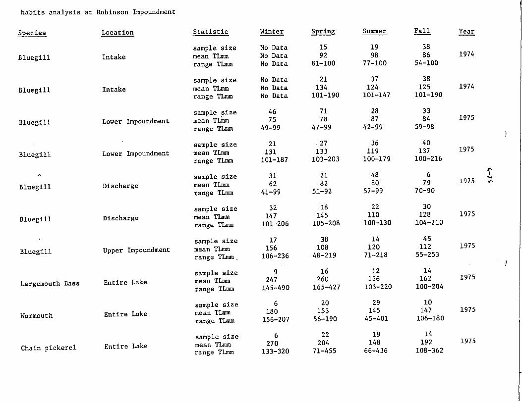
habits analysis at Robinson Impoundment

LocationSpecies

Bluegill

Bluegill

Bluegill

Bluegill

Bluegill

Bluegill

Bluegill

Largemouth Bass

Warmouth

Chain pickerel

Intake

Intake

Lower Impoundment

Lower Impoundment

Discharge

Discharge

Upper Impoundment

Entire Lake

Entire Lake

Entire Lake

Statistic

sample size mean TLmm range TLmm










Winter

No No No

No No No

Data Data Data

Data Data Data

Spring

15 92

81-100

21 134

101-190

71 78

47-99

S27 133

103-203

21 82

51-92

18 145

105-208

38 108

48-219

16 260

165-427

20 153

56-190

22 204

71-455

Summer

19 98

77-100

37 124

101-147

28 87

42-99

36 119

100-179

48 80 57-99

22 110

100-130

14 120

71-218

12 156

103-220

29 145

45-401

19 148

66-436

Fall

38 86

54-100

38 125

101-190

33 84

59-98

40 137

100-216

6 79

70-90

30 128 104-210

45 112

55-253

14 162

100-204

10 147

106-180

14 192

108-362

46 75

49-99

21 131

101-187

31 62

41-99

32 147

101-206

17 156

106-236

9 247

145-490

6 180

156-207

6 270

133-320

Year

1974

1974

1975

1975

1975 4-

1975

1975

1975

1975

1975

Table 4.4.2 Taxonomic list of items in the food of Lepomis r Robinson Imt indment. Seasonal occurrence in the food is indf. 2=spring, 3=summer, 4=fall)

-ochirus from various areas of ated for each taxon (1=winter,

Lower Impoundment

Cladocera Diaphanosoma (2,3) Eubosmina (2,3,4)

Copepoda Cyclops (2,3,4)

Diptera Ablabesmyia <2) Bezzia (2,4) Chaoborus (2,3,4) Chironomus (2,3,4) Cryptochironomus (3,4) Harnischia (2,3) Microtendipes (3) Pentaneura (3,4) Procladius (2,3,4) Pseudochironomus (2) Psectrocladius (2)

Trichoptera Oecetis (2,3) Oxyethira (2) Polycentropus (2,3,4)

Hymenoptera Formicidae (3)

Coleoptera Elmidae (2,3)

Hirudinea (2) Nematoda (4) Osteichthyes

Lepomis (2,3)

No. Taxa = 22

Cladocera Acroperus (1,4) Diaphanosoma (1,2,3,4) Eubosmina (1,2,3,4) Eurycercus (3,4) Polyphemus (1)

Copepoda Cyclops (1,2,3,4) Diaptomus (1,2,3)

Diptera Ablabesmyia (2,3,4) Bezzia (1,2,3,4) Chaoborus (2,3,4) Chironomus (1,2,3,4) Corynoneura (2) Cricotopus (2) Cryptochironomus (4) Dicrotendipes (2,3,4) Nanocladius (2,4) Orthodadinae (2,3) Orthocladius (2,3) Polypedilum (1,2,3,4) Procladius-(l,2,3,4) Psectrocladius (1,2,3,4) Pseudochironomus (1) Stenochironomus (1) Tanytarsus (2,3) Thienemanniella (2) emergents (2,3,4) pupae (2,3,4)

Trichopt'eia Oecetis (1",2',3,4) Oxyethira (3)

Odonata Didymops (2) Dorocordulia (2)

Hemiptera Formicidae (3) Myrinicinae (3,4) Pseudomyrinicinae (3)

Intake Area Discharge Area

Cladocera Diaphanosana (2,3,4) Eubosmina (1,2,3,4) Eurycercus (4)

Copepoda Cyclops (1,2,3,4) Diaptomus (1)

Ostracoda Cypridae (3)

Diptera Ablabesmyia (1,2,3,4) Bezzia (1,2,3) Chaoborus (1,2,3,4) Chironomus (3,4) Cryptochironomus (1,4) Dicrotendipes (1,2,3) Harnischia (3) Nanocladius (3,4) Orthocladius (3)

Paralauterborniella (1) Polypedilum (1,2,3,4) Procladius (3,4) Psectrocladius (1,2,3) Thiemanniella (2) emergents (2,3,4) pupae (1,2,3,4)

Ephemeroptera Ephemerella (1)

Trichoptera Oecetis'(2,3,4)

Odonata Coenagrimidae (3) Didymops (2) Enallagma (2) Libellulidae (3) Neurocordulia (1) Tetrogoneuria (1)

Hemiptera Corixidae (4)

S4, -&

Upper Impoundment

Cladocera Acroperus (1,2) Daphnia (1) Diaphanosoma (2,3,4) Eubosmina (2,3,4) Eurycercus (4)

Copepoda Cyclops (1,2,3,4)

Diptera Ablabesmyia (1,2,3,4) Bezzia (1,2,3) Chaoborus (2) Chironomus (1,2) Conchaplopia (3) Cricotopus (2) Crypotchironomus (1,2,3,4) Microtendipes (1) Nanocladius (1,3,4) Orthocladinae (1,4) Orthocladius (2,4)

-Parachironomus (4) Paralauterborniella (3)

,Pentaneura (1) Polypedilum (1,2,3,4) Procladius (1,2) Psectrocladius (1,2,4) Pseudochironomus (1,2,3,4) Rheotanytarsus (3) Stenochironomus (2) Thienemanniella (1) Tribelos (4) pupae (2,3,4) unidentified (3,4)

Trichoptera Agrypnia (1,4) Leptocella .(4) Oecetis (3,4) Oxyethira (1,2,3) Pharyganea (4) Pycnopsyche (1)

14 Lu

Table 4.4.2 (continued)

Lepidoptera Nymphula (4)

Coleoptera Berosus (1) Hydrophilidae (2) Hydroporus (2)

Hydracarina Hydrachna (2,3,4)

Amphipoda Gammarus (3)

Aranea (4) Nematoda (4) Oligochaeta (4) egg 'qases (3), Osteichthyes

Etheostoma-.(2) eggs"

Hymenoptera Formicidae (2) Myrinicinae (3,4)

Coleoptera Berosus (1) Hydrophilidae (2)

Lepidoptera Nymphula (1,2)

Hydracarina Hydrachna (3)

Amphipoda Gammarus (1)

Araneai (2,4) Nematoda (2) Oligocheata (2,3,4)

No. Taxa = 40

No. Taxa . 47

Ephemeroptera Hexagenia 1,2,3,4 Stenonoma 1,3

Odonata Didymops (4) Enallagma (2,3,4) Lestes (1) Libellulidae (3)

Hemiptera Corixidae (3) Palmacorixa (2) Sigara (2)

Hymenoptera Formicidae (2) Myrinicinae (3,4) Pseudomyrinicinae (3)

Lepidoptera Nymphula,(1,3,4)

Hydracarina Hydrachna (1,3,4)

Decapoda Procambarus (2)

Aranea (4) Oligochaeta (1,2,3,4) Nematoda (1) Ostrichthyes

Enneacanthus (3) Etheostoma (3) Lepomis (2,3) Notropis (2) eggs (2) larvae (2)

No. Taxa = 61

)

-4

)

- N

4-77

Table 4.4.3 Summary of the food habits of young-of-the-year largemouth bass (< 94 mmTL) from Robinson Impoundment from April to September of 1975

Spring Summer No. Per % % No. Per % % Stomach Freq. Vol. Stomach Freq. Vol.

Cladocera Acroperus 1.5 18.2 7.2 Diaphanosana 0.3 36.4 0.3 10.8 7.7 4.5

Eubosmina 0.1 7.7 0.0 Copepoda

Cyclops 0.1 9.1 0.1 7.4 7.7 2.1 Diaptomus 0.5 7.7 0.2

Diptera chironomid pupae 0.3 18.2 9.9 1.8 7.7 6.8 ceratopogonid pupae 0.1 9.1 0.9 culicid puape 0.1 9.1 0.3 Chaoborus 5.4 30.8 17.1

Ephemeroptera unidentified 2.0 7.7 7.3

Odanata Enallagma 0.2 7.7 6.7

Hemiptera Myrinicinae 0.8 7.7 6.7 Palmacorixa 0.6 36.4 27.7

Amphipoda Hyallela azteca 0.1 9.1 0.2 Gammaius 0.2 7.7 3.8

Decapoda Palaemonetes 0.1 7.7 7.7

Oligochaete unidentified 0.1 7.7 0.0

Osteichthyes Lepomis 1.6 54.6 53.4 0.2 15.4 12.3

Cyprinidae 0.1 7.7 3.1

Gambusia 0.2 7.7 7.1

Etheostoma 0.2 15.4 14.6

Sample Size Range (TLmm) Mean (TLmm)

11 48-92

61

13 32-94

74

4-78

Table 4.5.1 Back calculated length (mm) of bluegill collected from Robinson Impoundment during 1975 and 1976

DISCHARGE AREA

Sample Calculated Total Length at Age (mm) Age Group Size 1 2 3 4 5 6

1 47 65 -...

2 9 51 95 - -

3 6 50 89 120 -4 16 34 74 109 137 -5 10 33 65 101 132 158 6 5 29 67 92 122 143 170

Weighted Mean - 52 77 106 133 153 170 No. of Fish - 93 46 37 31 15 5 Mean Increment 52 25 29 27 20 17

LAKE ABOVE DISCHARGE AREA

1 2 3 4 5 6

1 14 62 -....

2 6 63 126 -... 3 7 45 84 133 - -

4 5 28 75 113 146 -5 5 30 60 93 137 158 6 3 27 63 90 120 147 174

Weighted Mean - 48 85 112 137 154 174 No. of Fish - 40 26 20 13 8 3 Mean Increment 48 37 27 25 17 20

LAKE BELOW DISCHARGE AREA

1 2 3 4 5 6

1 69 66 -...

2 19 53 94 - -

3 10 43 79 115 -4 31 35 68 106 130 -5 11 30 63 99 134 161 6 3 27 50 84 117 156 180

Weighted Mean - 52 75 105 130 160 180 No. of Fish - 143 74 55 45 14 3 Mean Increment 52 23 30 25 30 20•v •v

4-79

Table 4.5.2 Comparison of back calculated lengths of blue-gill from Robinson

Impoundment and from other similar lakes

Location

Present Study1

Lake Robinson 1968 (Phillips 1969)

Kitty Hawk Fresh Pond (Dickson, 1961)

Lake Waccamaw (Davis, 1966)

Lake Waccamaw (Louder, 1961)

51 n=276

50 n=33

56 n=8

36 n=8

43 n=14

Calculated

2

77 n=147

104 n=23

81 n=8

81

94

Total Length at

3 4

106 132 n=112 n=89

124 n=4

112 135 n=8 n=l

127 152

134 165

1 Weighted mean values from all areas

Age (mm)

5

156 n-37

198

n=l

178

6

174 n=ll

188

4-80 -•

Table 4.5.3 Total length/weight relationship for bluegills from three areas of Robinson Impoundment collected by electrofishing during 1975 and 1976

SeasonI Location

Winter Lake above discharge

Discharge area

Lake below discharge

Spring Lake above discharge

Discharge area


Summer Lake above discharge

Discharge area


Fall Lake above discharge

Discharge area


Number Intercept

27

851

13

74

251

42

67

179

48

87

377

- 4.603

- 5.077

- 5.380

- 6.270

- 4.922

- 5.179

- 4.836

- 5.420

- 5.732

- 4.537

- 6.451

- 4.981

Correlation Slope Coefficient

2.955

3.136

3.287

3.705

3.059

3.190

2.980

3.301

3.441

2.864

3.808

3.086

.970

.973

.963

.914

.962

.964

.926

.937

.951

.963

.950

.923

lWinter = December, January, February Spring = March, April, May Summer = June, July, August Fall = September, October November

- I

4-81

Table 4.5.4 Back calculated lengths (mm) of warmouth collected fromRobinson Impounament curing 1975 and 1976

DISCHARGE AREA

Sample Calculated Total Length at Age

Age Group Size 1 2 3 4 5 6

1 6 43 -...

2 3 31 59 - -

3 3 42 91 139 -Weighted Mean - 40 75 139 -No. of Fish - 12 6 3 -

Mean Increment - 40 35 64 -


1 2 3 4 5 6

1 3 53 -....

2 4 41 82 -...

3 11 42 78 120 -4 5 45 79 119 155 5 5 38 68 100 137 159

Weighted Mean - 43 71 115 146 159 No. of Fish - 28 25 21 10 5 Mean Increment - 43 28 44 31 13

LAKE BELOW DISCHARGE AREA

1 2 3 4 5 6

2 5 32 70 -...

3 4 45 90 135 -4 12 37 76 123 164 5 11 27 59 95 134 162 6 4 25 44 75 107 152 187

Weighted Mean - 33 68 108 143 159 187 No. of Fish - 36 36 31 27 15 4Mean Increment - 33 35 40 35 16 28

4-82

Table 4.5.5 Comparison of back calculated lengths of warmouth from Robinson Impoundment and from other similar areas

Calculated Total Length at Age (mm)

Location

Present Study1

Lake Robinson 1968 (Phillips, 1969)


Salters Lake (Louder, 1961)

Jones Lake (Louder, 1961)

Singletary Lake (Louder, 1961)

Black Lake (Louder, 1961)

1 2 3 4 5 6 7

38 70 112 143 159 187 n=76 n-67 n=55 n=37 n=20 n=4 -

43 89 132 165 n=25 n=10 n=6 n=1

41 n=2

33 n=10

36 n=8

43 n=6

25 n=1

86 116 135

69 107 157 193 234

86

66

251

122 180 205

122 183 213 231

48 99 150

'Weighted mean values from all areas.

4-83

Table 4.5.6 Length/weight relationship for warmouth from three areas of

Robinson Impoundment collected by electrofishing during 1975 and 1976

Location

Lake above discharge

Discharge area



Discharge area



Discharge area



Discharge area


Number Intercept

15 - 5.398

11 - 3.651

47 - 5.300

40

31

64

9

3'

14

33

6

41

- 4.677

- 5.774

- 5.591

- 4.315

- 5.636

- 3.669

- 5.387

- 5.035

- 4.875

Slope

3.315

2.559

3.286

3.003

3.484

3.419

2.859

3.435

2.565

3.299

3.181

3.079

Correlation Coefficient

.991

.947

.980

.997

.984

.990

.926

.999

.836

.843

.999

.954

'Winter = December, January, February Spring = March, April, May Summer = June, July, August Fall = September, October, November

Season1

Winter

Spring

Summer

Fall

4-84

Table 4.5.7 Back calculated lengths (mm) of largemouth bass collected from

Robinson Impoundment during 1975 and 1976

Age Group

1 2 3 4 5

Weighted Mean No. of Fish Mean Increment

Sample Size

3

5 5 5

DISCHARGE AREA Calculated Total Length at Age

1

105

44 43 33 51 18

51 43

2

83 93

105 94 15

44

3

130 137 147 138

15

4

178 209 194 10

56

IMPOUNDMENT ABOVE DISCHARGE AREA

1 2 3 4


IMPOUNDMENT BELOW DISCHARGE AREA

1

Combined No. of Fish Mean Increment

52 5

2

99 4

3

161 4

4

221 4

47 62 60

5

251 251

557

I

3

3 5

4

87

81 97 90 11

2

141 189 171

8

53

217 237 230

890 81

310 310

359 80

5

257 2

52 36

/-N

4-85

Table 4.5.8 Comparison of back calculated lengths of largemouth bass

from Robinson Impoundment and other similar areas

Calculated Total Length at Age (mm)

Location

Present StudyI

1 64

n=34

2 118 n=27

3 168 n=2 7

4 220 n=17

5 252 n=7

6

Lake Robinson 1968 (Phillips, 1969)

Singletary Lake (Louder, 1961)


Lake Waccamaw (Davis, 1966)

99 210 322 n=40 n=29 n=9

53 n=2

116 n=17

112 n-13

343

124 228 343 383 445 464

231 3i8 385 -

226 235 381 437 483' -

1 Weighted mean values from all areas-

7 8

480

4-86

Table 4.5.9 Length/weight relationship for largemouth bass from three areas of

Robinson Impoundment collected by electrofishing during 1975 and 1976

Season

Winter

Number

5

30

26

Location


Discharge area


Lake above discharge*

Discharge area



Discharge area



Discharge area


Intercept

- 6.153

- 5.102

- 3.073

- 5.615

- 5.108

- 4.935

- 5.292

- 4.851

- 5.234

- 4.887

- 3.827

Slope

3.559

3.087

2.252

3.295

3.115

3.013

3.166

3.011

3.148

2.994

2.572

Correlation Coefficient

.997

.978

.841

.987

.999

.997

.993

.999

.994

.961

.926

*Insufficient data to perform analysis.

'inter = December, January, February Spring = March, April, May Summer = June, July, August Fall = September, October, November

12

3

6

7

4

20

42

18

Spring

Summer

Fall

-N.

4-87

Table 4.5.10 Back calculated lengths (mm) of chain pickerel collected from Robinson Impoundment during 1975 and 1976

Age Group

1

2 3


Sample Size

5

5

- 133

DISCHARGE AREA Calculated Total Length at Age

1 2 3 4

130 136 133 10

103

224 248 236 10

79

315 315

5


12 3 41 2 3 4


9 17

6 4

126

119 127 113 159 126

3688

219 ý189 229 214

2739

LAKE BELOW DISCHARGE

1 2 3


5 8

120

1

120 120 120 13

2

223 218 220

13 100 92

232 284 253 10

81

334 334

4

3 4

312 312

8

4-88

Table 4.5.11 Comparison of back calculated lengths of chain pickerel from

Robinson Impoundment and other similar areas

Location I

Present Study 1 126 n=59

Salters Lake 170 (Louder, 1961) n=3

Jones Lake 132 (Louder, 1961) n=3

Lake Waccamaw 132 (Louder, 1961) n=7

'Weighted mean values from all areas

53

287 n=23

447

358

2

219 n=50

330

279

284

4

334 n=4

518

493

368

4-89-I

I

-I

I I

-i

1jj�Ii�i � -1 I � EJ I I I I H

�rj

a

R

- -I

:1

:1

S 4.

a

I

4.4

-4J

0.

WI-0 41

*1-4

*20 U

a2)0 .C 4

(1) 4-4

li -I

��'�/

4-90

Table 4.7.2 Numbers (per 100 m 3) of fishes collected in ichthyoplankton surface

tows in various areas of Robinson Impoundment May 1975 through February 1976

SAMPLING AREA ampling Month Period Lower Impoundment Discharge Area Upper Impoundment

ebruary D 0 0 0

N 0 Percidae 5.25 Percidae 3.34

[ay D Percidae 10.24 Percidae 3.27 0

N Percidae 30.63 Percidae 14.27 Minytrema melanops 20.16

Centrarchidae 10.08

rune D Percidae 1.80 0 Etheostoma sp. 1.58

Unidentified 3.60 Percidae 3.16

N Centrarchidae 10.80 Percidae 26.84

Centrarchidae 3.83 Centrarchidae 118.11

ruly D 0 0 0

N 0 0 0

Lugust D 0 0 0

N 0 0 0

;eptember D Percidae 3.02 * Percidae 9.41

N * * *

)ctober D 0 0 0

N 0 0 0

)ecember D 0 0 0

N 0 0 0

lo data available.

Ichthyoplankton entrainment at Robit.

Month

January

-f 4 .1 ______

Week nfrin 3n

1

2

3

4

March I- 1

2

3

4

May i

July

2

3

4

D N D N D N D N

" D

N D N D N D N

D

D

N D N D N

Number per

*

*

Percidae i 1.14

Percidae

Percidae

Percidae Catostomida Percidae Percidae

+ 41

2

3

4

5

i - - L

D N D N D N D N D N

Percidae

Centrarchidae Lepomis

1.48

6.91

.75

.75 18.77 10.08

*

.82

.85 2.56

ole 4.8.1

February 1

2

3

4

April 1

2

3

4

June i

2

3

4

August1i

2

D N D N D N D N

D N D N D N D N

D N D N D N D

N

D N D N D•

N D N

3

4

Percidae

Percidae Percidae Percidae Percidae Percidae

Percidae

Percidae

Percidae Percidae

Percidae Percidae Unidentified

Percidae Centrarchidae Percidae

Percidae

.87

5.61 49.37 3.97

.99 1)A no'1 . Ul '

1.13

1.17

7.71 I 24.59 -

1.18 1.03 4.42

3.78 2.52 5.63

9.32

-n Steam Electric Plant, March 1975 through Febi -ry 1976

Number

per Month Week Period Taxon 100 M

I

Week Period

)

Number Number per per 3

Month Week Period Taxon 100 MH Month Week Period Taxon 100 M

September 1 D October 1 D Percidae 2.12 N Lepomis 1.06

2 D + Unidentified 1.06 N + N Percidae 14.61

3 D 2 D Percidae 29.43 N Unidentified 2.35

4 D N Percidae 7.09 N 3 D

N Percidae 5.80 Unidentified 1.16

4 D N Percidae 5.87

5 D N Percidae 8.08

December 2 D N Percidae .960

3 D N Percidae 1.84

4 D N

5 D Percidae .73 N

*Sample not collected quantitatively. NOTE: Plant off line November 1 - December 10, 1975

+No larvae were collected in the ichthyoplankton net; however, 2-minute zooplankton sampling ( 3 0 0 y 30 cm net) continued 14.00 per 100m3 in the day samples and 2700 per 10m in the night samples

Table 4.9.1 Fishes 24 hours), December

Chain Pickerel Warmouth Bluegill Darter (primarily swamp) Other 1

Total2

Time Sampled

Chain Pickerel Warmouth Bluegill Darter (primarily swamp) Other

1

Total2

Time Sampled

Chain Pickerel Warmouth Bluegill Darter (primarily swamp) Other1 Total

2

Time Sampled

impinged on H. B. Robinson Steam Electric Plant Unit 1 intake screens (number and weight per 1973 - December 1975

Jan. Feb. Mar. Apr. May June July Aug. no/day wt/day no/day wt/day no/day wt/day no/day wt/day no/day vt/day no/day wt/day no/day wt/day no/day wt/day

.5 1 4.5 165

.5 48 1.0 49

48 hra.

.5 10 5.0 175

48 hra.

1.0 2 3.5 21 2.5 3 .5 4

• *' 7.5 30 48 hrs.

.5 63 3.5 444

32.5 827 .5 1

3.0 129, * * 40.1 1462

48 hra.

.5 2 35.8 236 7.3 5 3.9 38

47.4 281 49.6 hra.

1.0 3 5.0 36 3.0 2 1.0 9

10.0 50 24 hrs.

3.5 3 1.0 15 2.0 39 6.0 23

1.0 15 2.0 39 9.5 26 48 hrs. 36 hrs. 48 hrs.

1.0 1.5 3 1.6

10.5 92 116.9 .5

120.0 1618 46 hrs.

1.0 13.0

48

24 119

hrs.

631 3

983 1

.4 1.0

56.5 1.0

.6 59.5

120.7

161 7

529 1

15 712

hrs.

1.0 510

25.0

26.0 1026 48 hra.

.7 38.3

1.0 4.0

44.0 97

IA

101 396

11 10 508

hra.

*Data not available "2Totals were calculated independently thus rounding descrepancies may have occurred 1Includes white catfish, yellow bullhead, pirate perch, bluespotted sunfish, and bowfin

SI I 1 1 1 . 1 "

I.0% -4

-r I.0% -4

I.0% -4

516


Sept. no/day wt/day

Oct. Nov. Dec.no/day wt/day no/day wt/day no/day wt/day

Mean no/day wt/day

Percent Number Weight


1 '

Total2

Time Sampled

Chain Pickerel Warmouth Bluegill Darter (primarily swamp) OtherI Total

2

Time Sampled


1

Total2

Time Sampled

.5 * .5 65 .5 4 .5 1

2.0 70 48 hrs.

12.7 29.3

2.0 1.3

45.3 36

22 91

1 17

131 hrs.

.3 104

19.0 113 1.3 1

.5 2 21.0 221

94.8 hrs.

1.0 51.5

2 388

52.5 390 48 hrs.

15.2 .6

1.0 16.8

110 1

253 364

120.2 hrs.

4.0 262 211.3 690

1.3 216.7

36

258 1210

hrs.

.2 86

15.0 310 .5 1

15.7 397 96.1 hrs.

.1 2.2

8.4 75 33.8 .6 1 .3

.6 9.1 76 37.1

37 hrs.

1.5 1.0

31 1

2.5 32 95.2 hrs.

52 67

257 1

42 418

.2 89

.7 11 28.8 260 1.7 2 1.1 32

32.5 394

C'

f-I

0-4

U% r-.

V-1

<1% 6%

91% 1% 2%

<1% 2%

89% 5% 3%

12% 16% 62% <1% 10%

23% 3%

66% 1% 8%

&-. ! •D 4•

I

Table 4.9.2 Fishes impinged on the H. B. Robinson Steam Electric Plant Unit 2 intake screens (Number & weight per 24 hrs.) December 1973 - December 1975

Jan. Feb. Mar. Apr. May June July Aug. no/day wt/day no/day wt/day no/day wt/day no/day wt/day no/day wt/day no/day wt/day no/day wt/day no/day wt/dayChain Pickerel White Catfish Warmouth Bluegill Other 1

Total2

Time Sampled

Chain Pickerel White Catfish Wajmouth Bluegill Otherl Total

2

Time Sampled3

Chain Pickerel 1

White Catfish Warmouth Blhiegill 1

Other1

Total2

Time Sampled3

*1 Plant offline *2 Plant offline *3 Plant offline

Includes golden dollar sunfish,

,2.j

1.0 39.5

.5 125.5

4.5 171.0

48

235 1436

22 3991

169 5852

hrs.

2.5

.5 40.5

5.0 48.5

48

1.0 444 1.0 .5 7 ,10.0

1.0 119.5 1076 100.5

4.0 67 6.5 125.0 1593 119.0

48 hrs. 48

50 41

1672 408

2171 hrs.

954

ý365 57

1037 566

2976 hrs.

.7 208

.7 51

.7 53 39.1 1201 3.4 .43

44.6 1557 35 hrs.

6.8 1.0

245.9 6.8

260.5 49.2

328 259

2166 5.3

3265 hra.

3.5 1.5 9.5

96.7 8.5

119.7 47.9

1111 210

1636 2596

95 5648 hrs.

4.0 700 1.0 308

136.0 1608 4.0 83

145.0 2699 24 hrs.

86.0 2.0

*1 *1 88.0 12

6.3 - 5.7

4.7 '235.3

.5 *2 *2 252.5

46

May 6-30, 1974 May 2-27, 1975 November 1-30, 1975 shiner, creek chubsucker, lake chubsucker, spotted sucker, bluespotted sunfish, redbreast sunfish, pirate perch, flier, largemouth bass, swamp darter, eastern mudminnow, flat bullhead, black crappie, white crappie

1444 2

1446 hrs. 3

2734 177 538

2494 8

5953 hra.

2.0 2.0 2.5

240.5 .5

247.5 48

11.7 5347 1.0 21 4.4 331

414.9 2968

2.4 34 434.5 8701 119.1 hrs.

1200 100 220

3847 189

5555 hrs.

4.0 2.0 5.3

3382.6 1.3

3395.3 36

5.7 2241 5.9 42 6.7 775

855.6 7037 5.4 370

879.3 10465 97.2 hrs.

2050 134 337

10358 3

12882 hrs. 3

ToraIs were calculated independently thus rounding discrepancies may have occurred 3Additional sampling was conducted with fewer than 3 pumps operating, see Figure 4.9.I

PS o�.

U0

p,.. 0",


Sept. Oct.no/day wt/day no/day wt/day


1

Total2

Time Sampled


1

Total2

Time Sampled

Chain Pickerel Warmouth Bluegill Darter (primarily swamp) Otherl Total

2

Time Sampled

3.1 3.0 7.0

3586.5 2.5

3602.0 48

1159 10

399 11471

17 13055 hrs.

1.4 494 4.4 43 1.7 132

487.2 4907 2.0 72

496.7 5648 70.3 hrs.

.5 1.0

1093.0 1.0

1095.5 48

5 97

6190 19

6310 hrs.

Nov. no/day wt/day

2.7 22.0

4.0 496.7

3.3 528.7

36

1893 979 120

2765 235

5993 hrs.

Dec. no/day wt/day

7.0 2416 1.0 26 1.5 152

242.5 5364 4.0 164

256.0 8122

2.8 1.7 1.1

176.6 6.1

188.1 43.5

1274 102 140

1549 342

3407 hrs.

.5 3122.0 966 1.4 77

128.8 4.6

136.8

1867 582

3493

120.2 hrs.

58.5 5.5 *3 *3 64.5

1858 788 2957

48 hrs.

Mean no/day wt/day

1.8 6.9 2.9

851.2 3.5

866.3

830 280 279

4280 138

5807

3.0 1349 4.0 176 2.0 240

278.2 2702 4.2 308

291.4 4775

Percent Number Weight

<1% 1% <1% 98% <1%

1% 1% 1%

95% 1%

14% 5% 5%

74% 2%

28% 4% 5%

5766%'-,

ON

r-

Ln

,-I

4'

Table 4.10.1 Estimated total angler use and catch rate for H. B. Robinson Impoundment, June 1975 - June 1976

WEEKDAY

Season Location

AM Spring Upper Lake

PH

AM Discharge AM

Lower Lake AM PH

Summer Upper Lake PH

AM Discharge PM

AM

Lower Lake PH

Average Trip

Anglers Length

11 3.01 63 3.21

9 3.00 20 2.66

4 2.98P 10 2.23*

Estimated Total

Anglers

Total Hours Fished

WEEKENDEstimated

Catch/ Total Hour 1 Catch

151 455 .47 214 1276 4096 .21 860

195 489

87 291

585 0 0 1301 .51 664

252 0# 649 .41

0 266

18 3.03* 386 1170 .30* 351 10 2.36 275 649 .83 539

1 1.43* 13A 5.00

3 2.89 3 1.72'

45 64 .06# 169 845 .03*

4 25

67 194 .69 134 113 194 .06 12

Average Trip

Anglers Length

34 2.70 54 2.29

8 4.00 13 2.21

7 2.00 8 1.50

7 2.22 44 2.83

3A 3.20 5 4.13

Estimated Total

Anglers

Total Hours Fished

Estimated Catch/ Total

Hour Catch 1

327 883 .15 132 613 1404 .84 1179

52 208 .04 153 338 .32

8 108

91 182 0 0 139 209 .06 13

All Locations

82 182 .29 404 1143 .58

61 195 .63 31 128 .24

53 663

123 31

8 0.33* 630 208 0# 0 10, 2.61* 100 261 .04* 10

All Locations

Seasonal rotal

2385

780

279

3444

1606

183

156 " 1945 ko

1i

AM Upper Lake AM

PH,

Discharge AM PM AM'

Lower Lake AM PH

Winter Upper Lake PM PH

AM Discharge

PM

AM

Lower Lake PM PH

16 3.68 283 1041 .40 416 10 ' ý 3.24* 201 651 .24 156

3 2.25 1 1.58#

5 3.00 4 , 1.70

87 196 .65 41 65 .21#

108 324 0 153 260 0

3 0!48# 406 195 0# 17 2.00 553 1106 .29

2 3.80 10 1.41,

3 2.10 9 1.83

34 129 .24 461 650 .20

127 14

0 0

0 321

31 130

93 195 , .48 94 320 586 .27 160

26 4.10 ,47 3.56

8 1.74 12 2.50

6 3.29# 18 1.82#

25 2.19 32 4.71

13 3.74 21 2.50

8 2.12* 7 2.90*

165 677 343 1221

.22 149

.13 159 880

120 209 .27 56 288 125 313 .29 91

47 155 .17# 26 232 257 468 .44# 206

All Locations 1400

297 650 .08 52 177 834 .16 133

90 337 .23 218 545 .17

98 63

*Average of completed and partial trip data.

#Partial trip data only. 1 Catch/hour data are means of completed and partial trips. ATotal anglers interviewed during period (no anglers observed during instantaneous counts).

78 93

506

332

208 .16 33 183 .21 38

All Locations 1163 GRAND TOTAL 7952

,Fall

Tag Number Date LocationTaggedRecapture

Length Weight Date Location Length Weight Comment

Warmouth

Largemouth Bass

Chain Pickerel

Bowf in

Yellow Bullhead

Flat Bullhead

80 400 667 839

870 873 874 874 914 996

661 697 713 796 798

644 649 787 984

955 986

87

861

119

6/25/74 6/25/74 2/10/76 2/13/75

2/6/75 2/13/75 2/13/75 2/10/76 4/30/75 2/13/75

2/10/76 9/26/75

10/16/75 2/11/76 2/11/76

1/12/76 1/13/76 2/11/76 2/20/75

5/13/75 2/20/75

6/26/74

2/5/75

2/13/74

G-1 A-i A-i A-i

E-1 A-3 A-3 A-3 E-1 A-i

A-i A-1 F-3 E-i E-i

E-I G-3 E-1 E

J E

G-3

A-3

G-3

184 145 163 185

178 180 170 180 163 170

241 240 337 200 224

446 460 390 264

612 604

292 283

334

120 45 86

140

115

110 124

85 120

158 146 565

95 122

439 820 290 100

2550 2040

330 355

638

8/28/74 G-1 4/2/75 A-i

2/15/76 H 5/20/75 Canal N. of

A-I4/5/75 4/2/75 2/10/76 3/24/76 5/9/75 7/5/75

2/13/76 10/14175 11/18/75 2/25/76 2/25/76

2/29/76 2/29/76 2/29/76 4/2/75

6/11/75 6/18/75

11/2/74 4/9/75

A-3 A-3 A-3

190 160 164

182 180 182

145 89 88

146 124 124

A-I

N. of B-i S. of C-i

F-3

N. of G-3 E-1 cove

E-3

J E-3

N. of G-3 F-I

280

627

120

Angler Return

Angler Return

Angler Return Angler Return

Angler Return'Angler Return Angler Return Angler Return Angler Return jo

Angler Return Angler Return Angler Return

2724Angler Return

Angler Return Angler Return

Angler Return11/15/74 G-3

A-I 213 182 2/10/76 A-3

Tagged

Redbreast 641 1/12/76 212 180

'4' �-• 4-99

Table 4.13.1 Common and scientific Creek during 1974 and 1975

Common

Bowf in American eel Redfin pickerel Chain pickerel Golden shiner Dusky shiner Unidentified shiner Creek chubsucker Lake chubsucker Spotted sucker White catfish Yellow bullhead Tadpole madtom Margined madtom Pirate perch Lined topminnow Mosquitoefish Mud sunfish Banded pigmy sunfish Black banded sunfish Bluespotted sunfish Redbreast sunfish Pumpkinseed Warmouth Bluegill Dollar sunfish Largemouth bass Sunfish hybrid Swamp darter Tessellated darter Sawcheek darter Piedmont darter

names of fishes collected from Black

Scientific

Amia calva

AnEuilla rostrata Esox americanus Esox niger Notemigonus chrysoleucas Notropis cumminsae Notropis sp. Erimyzon oblongus Erimyzon sucetta Minytrema melanops Ictalurus catus Ictalurus natalis Noturus gyrinus Noturus insignis Aphredoderus sayanus Fundulus lineolatus Gambusia affinis Acantharchus pomotis Elassoma zonatum Enneacanthus chaetodon Enneacanthus gloriosus Lepomis auritus Lepomis gibbosus Lepomis gulosus Lepomis macrochirus Lepomis marginatus Micropterus salmoides Lepomis sp. Etheostoma fusiforme Etheostoma olmstedi Etheostoma serriferum Percina crassa

Station J Bowf in Redfin pickerel Chain pickerel Golden shiner Dusky shiner Creek chubsucker Lake chubsucker Spotted sucker Yellow bullhead Tadpole madtom Margined madtom Pirate perch Lined topminnow Mud sunfish Banded pigmy sunfish Black banded sunfish Bluespotted sunfish Redbreast sunfish Pumpkinseed Warmouth Bluegill Bollar sunfish Largemouth bass Swamp darter Tessellated darter Sawcheek darter

1976 Jan. Feb.

18 4 2 8

2

2 2

4 6

1975Mar. Apr. May Jun. Jul. Aug. Sep. Oct. Nov. Dec.

2 2 12 2

2 20

26 46 4

4 8 4 4 2

6 2

4

2

4 12

4

4

4 4

2 4 2

8 20 30

4 4 6 4 2 2

2

2

2 2

2

42 20

2 2

30 10

8 6

4 6 46

2 2 6

8

2 8 10

2 16 2

6 2 2 2

4

2

20 2 8 8

2 2 8

6 2

6

22 4

22 30

2 6

20 22 14 4

40 138 8 26 8 8

22

8

4 8

6 2 6

2 10

8 6 4 4 4 2 2

2

11

6 2

4 8

8 14

6

2

2 6 4

4 10

6

2

2

4 4

6

4

2

0 0

2

8 2 2 2

Table 4.13 (

1976 Jan. Feb.

Station H American eel Redfin pickerel Chain pickerel Golden shiner Creek chubsucker Lake chubsucker Spotted sucker Yellow bullhead Pirate perch Banded pigmy sunfish Black banded sunfish Bluespotted sunfish Redbreast sunfish Warmouth Bluegill Dollar sunfish Largemouth bass Sunfish hybrid Swamp darter

Station K American eel Redfin pickerel Chain pickerel Golden shiner, Creek chubsucker Spotted sucker Yellow bullhead Pirate perch Banded pigmy sunfish Black banded sunfish Bluespotted sunfish Redbreast sunfish Warmouth Bluegill

4

6

6

4 4

4 18

2

2 2 6

4

2 2 2

6 26

2

2

1975 Mar. Apr. May Jun. Jul. Aug. Sep.

4 6 10 10

2 10

4 26 2

2

2 32 24

12

2

4

2

2

2 6

4 14

4 2

2

4 2

2 4 4

6

2 2 2

8 2 4

2

Oct. Nov. Dec.

10 4 2 2 2

4 2 4

2 2 10

2 2

2

4 2 2 6 6

50 126 2

6 8

6 24

4 14

2

22

24

4 92

2 70

4 2

92

8 14 12

10 12

4

3 3 3 6

8 22

2

2

8 2 6

4 12

6 2

2 42

2

I

4 2 22

2

3

22

2

2

2 2 2 172 6 10

2

(continued)

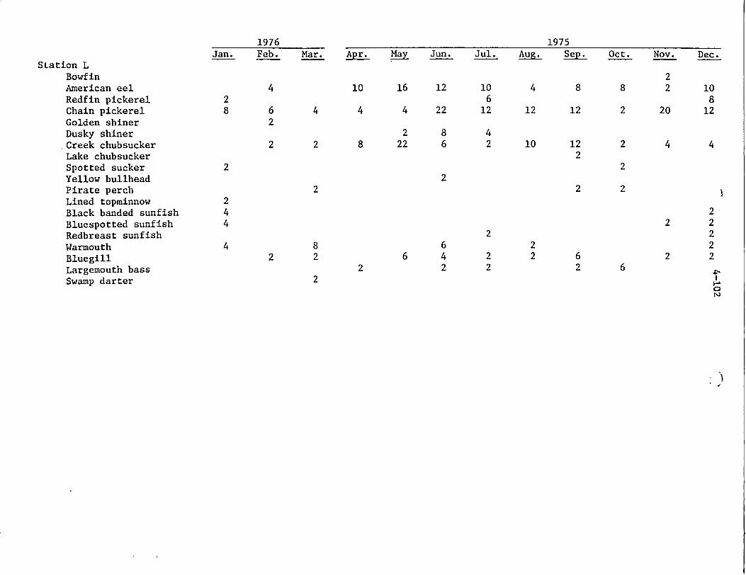
Station L Bowf in American eel Redfin pickerel Chain pickerel Golden shiner Dusky shiner Creek chubsucker Lake chubsucker Spotted sucker Yellow bullhead Pirate perch Lined topminnow Black banded sunfish Bluespotted sunfish Redbreast sunfish Warmouth Bluegill Largemouth bass Swamp darter

1976 Jan. Feb.

2 8

2

2 4 4

4

4

6 2

2

2

1975 Mar. Apr. May Jun. Jul. Aug. Sep.

4

2

10 16 12 10 6

4

4 8

4 22 12 12 12

2 8 8 22 6

4 2 10 12

2

22

8 2

2

6 6 4

2

2

2

2 22

Oct. Nov. Dec.

82 2 10

8 2 20 12

2

2

2

4

2

2 2 6

2

4

2 2 2 2 2

0

26

?

4-103

Table 4.13.3 Numbers and weights (per hectare) of fish collected from Black Creek

during August 1974, and August 1975

1974

Species

Redfin pickerel Chain pickerel Golden shiner Dusky shiner Creek chubsucker Lake chubsucker Spotted sucker White catfish Yellow bullhead Tadpole madtom Margined madtom Pirate perch Lined topminnow Mosquitofish Mud sunfish Banded pygmy sunfish Blackbanded sunfish Bluespotted sunfish Redbreast sunfish Warmouth Bluegill Dollar sunfish Largemouth bass Swamp darter Tessalated darter Sawcheek darter Piedmont darter

Total

Redfin pickerel Chain pickerel Yellow bullhead Pirate perch Lined topminnow Mud sunfish Blackbanded sunfish Warmouth Bluegill Largemouth bass

Total

Station No./Hectare1975

Kg./Hectare

J

2257.3 250.8

35.8 35.8

107.5 537.4 859.9

3081.3 788.2

71.7

107.5 •322.5

179.1 394.1 215.0

35.8 35.8 71.7

537.4 286.6

71.7 250.8

10533.9

1.5407 0.5016

12.8986 5.2311 0.0717 0.2508 0.8957 0.8957 1.4690 0.0358

0.0717 1.1824 "0.6449 2.6514 5.0520 1.4690 0.2866 0.3225 0.2508 0.4658 0.1433 0.2866

36.6177

H

35.83

17.91

35.83 4030.82

17.91 4138.31

0.2687

0.0358

4.8728 22.7338

0.0358 27.9470

No./Hectare

119.43 457.82 59.72

3244.56 199.05

19.91 19.91

159.24 696.68 218.96 418.01

99.53 19.91

139.34 39.81

776.31 199.05 199.05 119.43 119.43

99.53 218.96 59.72 79.62

7782.96

17.91 17.91 53.74 89.57

17.91 17.91 53.74

1791.47 35.83

2096.03

1975Kg./Hectare

4.3792 34.2172 0.6768 2.0701 0.4777 0.8559

18.9697

T0.3981 0.5175 0.3981 0.9156 0.3185 0.0199 1.9905 0.0199 3.3640 0.6370 9.2360 0.5573 2.1896

0.9754 0.1791 0.0995 0.0398

83.5026

0.0537 3.4934 3.8875 0.5016

1.0391 0.0179 8.4737

27.3917 1.4511

46.3096


4-1041974

Station No./Hectarecies Kg./Hectare1975

No./Hectare Kg./Hectare

:ican eel Ein pickerel [n pickerel Low bullhead ite perch ad topminnow quitofish sunfish

Akbanded sunfish aspotted sunfish breast sunfish nouth agill lar sunfish gemouth bass np darter salated darter cheek darter

Total

K

K (cont'd)

35.83 17.91 35.83 35.83 17.91

143.32 17.91

35.83 35.83

3117.17 35.83 17.91 53.74 35.83

3636.69

3.6188 0.0717

10.1039 0.0896 0.0358 0.0717 0.0179

0.0175 0.1433

11.5013 0.0537 4.2637 0.0537 0.1075

30.2401

95.97 76.78 57.58 38.39

19.19 115.17 38.39 19.10 76.78

652.61 19.19

19.19 19.19 19.19

1266.83

0.6526 7.7737 0.0768 0.1727

1.2092 0.3071 0.1152 0.0192 1.6699 3.4934 0.4223

0.0384 0.0384 0.0192

16.0081

A

4-105

US 1

Blak\Creek

Transect J

SR 346

XxUA*

C

Dischdrga

AH B Robinson Ui

0 Y.

-Scale in' Miles

LEGEND

£ Gill Nets * Wire Traps m Electrofishing * Rotonone U Larval Traps a Larval Tows x Seine

R 39

-23

Traris,,ct L

Figu•re 4.2.1 Fisheries sampling stations, Robinson Impoundment'

"A-

,S

4-106

��*1 1

4

I

I--.

LEGEND

A-1 A-3 E- 1 E-3 G-1 G-3

.40

44 * .

i/ � A/ /

i.

* 1

* August data not available

Figure 4.2.2 Shannon-Weaver diversity index of

Impoundment during 1975 and 1976

fishes collected from Robinson

i

l

.. I.. .

i! L,

4-107

- . I * 2

-. ,- I

0SPERICENT VOLUME,20 40 60 80 I1IIIIIII

0 0 1PERCENT FREWUENýY_ 20 40 60 80 100

I- I I I I I I I I I

.- SPRING

..... -CYCLOPS .

- CHAOBORU$- ...

.DECETIS.. 4

POLYCENTROPUS

I . I

80.0

14.1 . ...

1Q.4 , -

.1...

DIAPHANO$QMA

- ..EUBQSMINA_ .

CYCLOPS _..

.CHAOBORUS.

EUJBOSMINA

+ SUMILER ... " '

13.~~ ~~ 6o_ r._ ..80.0

* s.:.... ,52.6-20.5

LL

80.2

Figure 4.4.1 Percent of total volume and percent frequency of-occurrence of the major components in the seasonal food habits'of the bluegill (<100 mm TL) at Robinson Impoundment in the immediate vicinity of the intake structures during 1974

M 20,0

. 13.3

92.1

lllllll';'-I I

-5•2.0 _.

-- t --• - F-

I I

4-108

PERC ' V l 1-PiRC-EW F IREM, iY.1.

2R0 86IU '1 3 d 1 '4

.QECE = 7.5..

- "I -I ---

-B 57i! ... ._7...

OECE~u ~7.3'. A--- AXL

- , , *,,

I. , - + ,

EJBDSM I a •-a--

CHINOMUS r2.8! :Ti

PRQhi I - _

igure 4.4.2 Percent of total volume and percent frequency of occurrence f the major components in the seasonal food habits of the bluegill > 100 mm TL) at Robinson Impoundment in the immediate vicinity of the ntake structure during 1974

4-109

*1.

.1

IL..kI

. . ... I|-.

, "; -I

.. .... +.....! 'E ' S I ,

• " ' : " I .. .. S ...PQLY~Ws M 2...

PUPAE' I

4 4 - *1--'

-- TDLAP-HAN

S..... AiOBQ

• MYR IN IC

L. BIL6� -;

- - .- i*- 17 .7

I. I 4.� -, 'sP

36.1

I T

. -- •- -. 4----•-- 3 .I_ -... .

I * ,

-. . zL , ..... ... 1 .I .. , ..7_ M ,'1" ] "

- Il.•

M4-1

S" I I

.... = _i mm , ;

_.• . . I... '

-- EURYCERChj&P j

Y-I

,ABLABESMYIA.

----.i~mY • , -_

--+--SLJM

* . *1

F. A

-~I

"-+7 F

SI7

JIER

-99.4

- I,, -

-- -P- i- ---- 2f 4 8) -j

:ING

.63A4

! ' -

• . I + i .

: " 46.4 ..J *' - ._ 5. . . . . _

L-t.

_10 il , !

I I

. . , . . ! - I , •

Figure 4.4.3 "Percent of total volume and percent frequency of occurrence of the major components in the seasonal food habits of the bluegill (< 100 mm TL) at Robinson Impoundment along Transect Aduring 1975

.j i

+ + l I I ........ .• - "p---'• ..... U •-U=.m•, __

. . . , , , = ! ,, i I ,

.---- ___. ...... z -M--•i--m mm-... .

I

!PUPAE

I I I

L •

4-110

.2 . -K I..-i i� .f.

-. _,~E1 IO M1NA_

I IPP~

_ DIAPI1ANOSiQFAA

-. POLYPEMIUM--

CI-IACQHQUS

:MYRINICINAE

EUB6.SMINK. 4-

EURYCERCUSL.

!-CYCLOPS

- ABLAaESVELA

.__._CH1RONOMUS_.___

PQLYPEPUUM-

. 041) do. 6o1(

*I I

121~

SPJ

143-

I .

�19.5� ---A--;-I . I-l

I ffiSIJM

U--.

.15. 9

9 1

9 6;,.

a-4.6

V...

1�

II

* . I * pI:g1'IMrrRRFnIIFNI

o 2o 40 '9

�Rq�

UNG_

-~4 ....

- .4--

33.3 i

I ? -�

M M.. !132.5

!i 0.0 1

.1 A.

I.

-- I-

i _C Q.

-I .�1

-. 1-4 -

I I 1

H -i- . A.

'igure 4.4.4 Percent of total volume and percent frequency of occurrence f the major components in the seasonal food habits of the bluegill > 100 mm TL) at Robinson Impoundment along Transect A during 1975

I-.

I..

1��-

.1-�I-

I.

LTUR

IV -1E1Q.2,1KOX9.12ZM

IAý

20.01

...... :FFQCLAD1 S

4-111

.. _ - . . _-.

. --ýYCLbR--

-------- EUBOSMINA-.. - .C .......

. ! IP I-

I

'flHAOHAERIIS

I l I O• IN.

I I

--- .-. * .:.... r ---T

"--1- (.............

1 , 1

I-. . I�I*

'4.�MIIB I 4 1 I

* 4

w

r

I--. I . . . ;- 1 , 4 , . i ' s.

F- __

M A-

Ii�I "-��

I -:

4..'

-4 y P iE~~LEC

m i i I J i I

.4_ --

4 I

:I 9 w

TERI

--•'•: 4' •+m

II

-. ... +.

dER '

2L L

-- - j.+

70.8_---

.4 4

I -

.1

- 4 -+ 4.L.. 41

Figure 4.4.5 Percent of total volume and percent frequency of occurrence of the major components in the seasonal food habits of the bluegill (< 100 mm TL) at Robinson Impoundment along Transect E during 1975

I 2F 4t rI

II. J

4 0 I r

i~z i " -

i2

' 1X.

-- ; • +, ,

44. .. . -II- s. um...

In .. . . .. .

! ;° : i

- I1-

4-112

I -- -- i--*-'.

I;,T

-* M IFUI IBM" . ~ -10.4~

.1 . 7 H- Lit

____ ____ ___

I -.

MYUIA~iANGMAE 7. 10.4

F- -MERGENT I.-.

- IT

- i - S - 2-1- - - -' *'

liue4.. eretofttl oue n eretfrqecyo ccrec

)f ABOU t1he majo copnet intesaoa odhbt ftebug >~~~~~~~~ 10 mTL t......mondetaln.rasc Edrng17

4.411

I I*I

*.J

-.-DWRlT~iNQi.ES--

TYC-NOPSYQ1E-- *

.:UA .7

*IHEXAGENJ{:

.JHYDRACHNA& I 42'

.OLIGOCHAETA 11 V

* EUBOSMI~i 631 d

.1

EXAGEN 1-4 .Z.

*..OLIGOCHATA-. t- 74A!

*. ENNEACAN'm 16US

E UBOISMINA

IEPHEMEROPTI .5A

I(- I

LLM12IL!4JJ±

14' 253 I2

-wl 7-

.3

0I :16.5~ 4 -L ..

* 24.J

MENE.1 I

R i4 .i~i

* i~28.6j.

-j

A I I

j.

-- 4---.-

* -I I

.1.---- I

14-A

>I~tLE7

Fi~gure 4.4.7 Percent of total volume and percent frequency of occurrencie of the major components in the seasonal food habits of the bluegill at Robinson Impoundment along Transect G during 1975

T -1

* - I

__J.ADCiNA,

.I pnMugaI-

4-114

21.74

A

*.NO.MIROPIERS 1--.5

_UEtDFNTIFiEDP1-f

* .LEPOMIrt-

PROCAMBARUS

ETHEOSTOMA

LEPOM11S

* UNIDONTIFIED-FI

* I

* I

-- --.---.

A 1 . -

.I

I I *~~

E&X*.4 20.

R-7.5 1.6I

t

ING.L.F

AEJL .~. 31.34-4

-- '-I.

��1�*��

-Ha. AX-A.. iL-'

�*1 * I

* * *

I .. -

* �1��

* I.

I.

I* I * . 4.-

* *1��

I I

-- T

igure 4.4.8 Percent of total volume and percent frequency of occurrence f the major components-in-the seasonal-food habits of the largemouth bass t Robinson Impoundment from all transects during 1975

-L. 0ý033-3

35L7

- - 4

I

4-115

7 .

"* I "-- * ' lARAI'" - I'- : +

-- ;W MOR

-.

I I

PROCAMiSAR"S "-- -I .. .. ..... t•DYMDPS .. ..~

* I

. -. . ...

LL-- M IS--ý

"*- I= I

, I

-1 .. . 1"

Pnct S, P -M --- L

2b 80'.- i.0 C

11 T-1A) BI .I I

P1 0V d- 2

." ._PIi ' , an i * 0.

J I T-.i

BCE mt.EREOea NF d:Y - ... . L+,tiLL ,!LJ+ -..

TERl. .. . . .

, _ _ , -. .

-7. I i• - I

SUMMER S . 36.7

* I . - . .. .. . 1

I.-

-I

0~

iT d -"

.1

.. .. . 1. . PAL *-4' .__._ . .. L .. . .. FA L -.- -L-L 7

"r" " "i ' , ' ':€<,• 'i• ••.'

MUM -77- r MUM 7+

Figure 4.4.9 Percent of total volume and percent frequency of occurrence-. of the major components in the seasonal food habits of the warmouth at Robinson Impoundment from all transects during 1975

i I

I

I

r I 13.8

O M.M i 37

I

ii1

q

Ii m . . . . . . . .

-- ZEII

f-

I

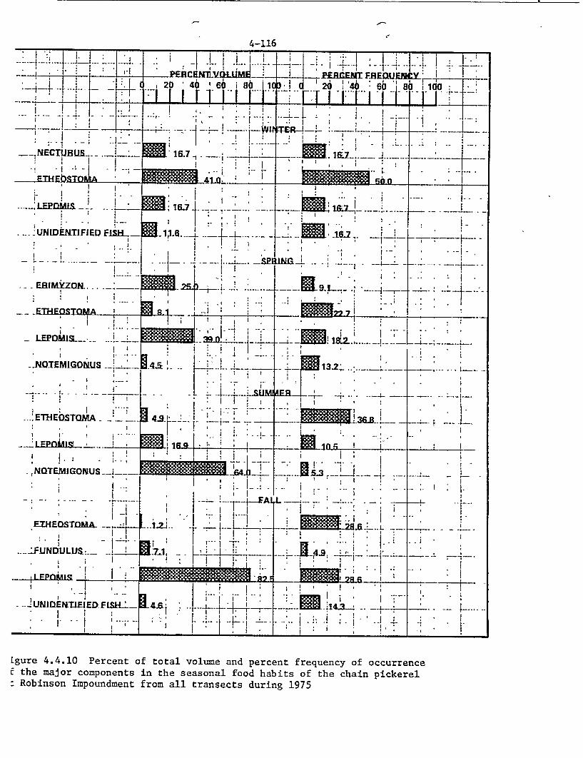
I *.'

_IN ECT-UBUS..

'2LEPOMIS9 I

-UNID6NfFIED FISH-

--- EEBIMkZIYQL.

- .DOTEMIGO'NUS

-'EThEESTOMA

I

-NQTEMJGONUS--1--

EI.HEOSTOMA.

-..-.:fUNDIJLUa.%!

UNIDiEMTJED.FISHL

4-116

41 1611

16.7 16.7 -

I-

R16-

-45 7..

) -

--SPI

-- S I -

I. -

.1,

-"i4 * *-i-----1--� * PERI�E&I F.RE�2U�

f2� [1' IF ''AJI 6h �a

+ji�v.') i 10'

I- I Y I �..4. 4. -

-.- .* -

± -

I * I

* . i:�flfl

K I .

UNWL. . -.i--�:- -. �

* 2211

MM.

&ERf-1-4 -4-

In �

1 : 7

�0�):

AF.;I

.1

- . i�a�

114.1 -L

I,

-i -.

.4- --

Lgure 4.4.10 Percent of total volume and percent frequency of occurrence E the major components in the seasonal food habits of the chain pickerel :Robinson Impoundment from all transects during 1975

- I- -

- I

- , . --I ---- 1-* . I

* I

* I

- I

-4---.

I -.-- � .- L.

* I

* I-.

* I

1

* �1��*14.6i

ETH

ETHEDSTONA I A0 R171

4-117 Figure 4.5.1 Length frequency histograms of bluegill collected from Robinson

Impoundment from April, 1975 through-March, 1976 with larval fish traps and

electrofishing I

20+

15. at. I t

tii

lott

Itic i

1 2 3 a 5

5 5 5 5

I ci.•

tiAl iii

Getti April

e tC l

7t, t r qt 0 2 3 ccc c cii tc

cii i etc itt etc ciil eecic etc iiiJ•

ccc cec etc tie iii ite tii ltt

act tic 1iii eec tie tie ere tie iee ee cit

ties iee cit% etc ee tie elic, get *eti tte cit

--------- ~~~~~----------------------------------6 7 b Q a 1 3 U 5 6 7 • 9 o 1 2 3 '"

b 5 5 5 5 S 5 5 5 5 5 5 5 5

•qIDPLUNT OF'10M4• SiZL GROUP

145+

I i

Iit

I ***

I itt

35+ ***

I ,iii cii

l oit a it

I iii iIII2

55 5* -5 5 5 5 5 5 5 1

I Ofi Sit t o G Ha7

I cci itlt l

I lii ice #I

• .etc ice Jl

I el t tit-eit t

I iitt t i tllllt 9

| i~~l itc ict l ti

I Nl t ee i tee l itltit I iii

-c1

I.....................et-----,-,-,.t.......... .. ... .

5 • 5 5 5 e c cii • 5 5 5 5 5 5

£5 tie, . • iP TTO ii •• I•U o

dflfli' 3Ztg pwwo, 40 LNIfldOIW

SO SO SO So Is 9 * so SO I I I 1 * 4 0 S £ S S 5~S S~ S S S~S S S S S S ~ l ~ ~ 4 ) 6 1 S 1i f

6 9 * 9 9 9 9 f9 0 ~ 4W s 9 s 9 09 fW .s0 4 V q

S94 49 09 9 9 9 9 9 9

9WW ~ ~ ~ ~ ~ ~ 4 99 9 95 99 9 w9 *

few V* 99 9W99 *4

999 49 999 9* 4 999 99 9W 599944f

999l! 9919 999T .50 INnd

S , S S S S ~ ~ S SSS S S S S S q

-------------------------------------------------- ----------------------------49 v* 69 999 *9 59 *9 99 * 9 * 9 99* 4 94 v4v4 49 9

9*9~~~~ ~~ v9 44 v~ 9 9 99 9

9*9 99 99 99 95 99 99 59 so

9* 9W 4* 9 9W 99 9

2S '7

S

C-

-... .. .. ..

599 99 9V9

(panupauoo) Togov 9-.ZT1a

Figte 4 . 5 .1. (continuect) 4-119

30,

asat.

I ** *

Rik * **

at*A I a..

I tat I at.

I I I1t, t tatat

IS

I At

, k

1 1t at AugI I I- ? 2t

I 2aa I sea

I t** ae et leta I **te .e *i t..

ea tt atta ate ala t,,a, I t t t c as. a., t t.,,, e~ at. et

I 1 I 1 j I I 1 1 1 2 2 2 2 2 I 2 3 'I 5 • 7 8 9 (0 1 2 3 i• 5 6 7 8 0 1 2 3

5 5 5 5 5 5 S 5 5 5 5 5 5 5 5 5 5 5 5 5 S $ 5

MIDPUTNT OF 10mM SIZEý GRUUP

20,

I att tat

eat, tt ,t September

I tat tat tat

I ea te tat tai t*

e •el ta at. tat -l i

I tea ta lt tat eta Ita tat 5+ sa it al•te tat eta tat tat

I i tat eat tateatl l tat ellta ateltt

I ~~te taIlIlt tat ietc tee tat Ca. eta lta lttt tat

tttt att tit ate ia ttat tee eet etateta at.tta.

1 2 3 '* 5 '• 7 8 q o 1 2 3 £1 5 A 7 8 Q 0 1 2 3 'J 5 a a . 5 . 5 e a a 5 a .S ~ a a . e 5 5 .5 5.5 ,s .5• ,5 5 5 5! 5 5

MIDPOTNT Of 10OM,$IZI ,GRUUp -•

Figure 4.5.1 (continued) o - 000 4-120

0*0 000October

"A0 *00

A,0 00 A*0

70 00 000 7 A Q

*0*1O 0* *a0** 0ovm0e

000 000 ,No* of*0 *0 0*

I I I I I I I I 1 1 2 2 2 ;. ? 5 7 8 q .1 1 2 3 5 6 7 a 2 31 1

5 5 5 S 5 5 5 5 5- 5 5 5 5 5 5 5 5

mIDPUINT oF IOMM' SIZE GROUP

*00 00* 000DNember

*0 *0 a0 Al00

... .. .. .. .. .. ... .. .. .. .. .. ... .. .. .. .. ..*.. .. .. .. .. .. ... .. .. .. .. .. ..

I* I* I0 I0 I00*I 1 1

1* 2* 30 00 a 0*0l

50 00 s* 000 0*0r

000PTM OP* 10M" SIZE 0U11P

A-

Fieure 4.5.1 (continued) 4-121 20#

S*** **January

I tIe ti aee

I **i A 1* tl e al t at ht

B .ah Clh *** *** *i hth *0t

I ha a.. ihh Aii *lA i*i hat A*a 0* *

B ili aca pil liCta ha ill hh lt Il

selt l t 014' *&t *** *** 41110 *** *** B .al hahil at aol all at ace al altie

----------------------------------------------------.......................... ................................ I I I I I I I I I 1 ? 2 2

1 2 3 '1 5 6 7 8 9 O t 2 3 4 5 6 7 9 9 C I P ! a S 5 5 5 5 • S 5 5 5 5 5 • 5 5 5 5 5 5 5 5 5 5 5 5

M!1PUINT OF 10MM SIZE GROUP

Zn,

B aaa February

10+ a h h h a

/*Al

1 et Ca ,a 9 h 1~ 2 eac67 9

S.C CC h5 a. 5hi ha5

Bot OFl II e lt ICC SIZ GRUUt

ae a th ee *1aaae .a*

iih h Ct. C llt hht Ia. ICChh

I ith4i ia ll lt hAg a'. 1el

ah et h lhC Ie. ill .a. laC a.. **a eh a hhaa i t

I I I I I I I 1 1 1 2 2 2 2 2 2ll

C C C C C or & * CA * ** * **C C * C * C *

•i ttl !~titt l t o il tee ltil

t It* tail Cft I*t & o

0+aat ..................................... et..................

I CCC l il i ha. ett iti teC CIl t

I *iail ltit itC CCC ha. ICC tal aaat ttil i t

I I I t I et 1 1 2 2e? 2 2I2

1 2 3 4 ea 9 e al 3 a7 '8 9 t 1 a 3

5. s5 5s 5 5 5 5 5 s s s 5 s r, c; 5

I *Ch ICC *C CC el ec ta al iC ha. I•• * o

CC tCC.ec e ltl tht 4th l e t a

B I c C C i~ IC C itCAi hCC ltiathO I ta

1i l l 1t It I I I , 1 1 1 2 2

1 3 't 5 8l 9t tt fi ?t 3 7 8ll

S 5 5 5i 5l 5l 5t 5t 5i 5i 5 5 5 5

C C Ci Cl Cl Cl Cl Cl S~ tt C C Cl

MICPUTNT OF 10M 317E GROUP

30000.OuOOf

2OO0.o00000

"1400u.00000

o0

14.

U.4

0

w 1-

-2000. 00000

4.

4.

A I ha

A

4

13-,.UOUuVOUU 15t.sU000OuOb 18Z.*000 UUO z0b.O0000000

LL6LhL1 A - I UdS . b - O 8 , 1l(..

Total length in millimeters

Figure 4.6.1 Relationship of the number of mature eggs and total length of Lepomis

macrochirus in Robinson Impoundment

O000.00000 4

IA

A

A

A

A

A A AAA.

A

AA

A

AA

A A A

A A A

A

A AA

tb.u0000000 11O.UO00OUUV

A

40U00.000-Jo +

30000. OOOC.

2I,0juu .0g0Go +

IA (,.DMOGuO +

I-

A

A

A A A A-

k('4.UOUUGUO0 lI e.00000000 1;12.(,OOOuOO(u ITb.00000000 2.0.OiOOOOuO U24.00000000

LkGtIUt A - I. 0S a 6 - Z UbS . -1L.

Total length in millimeters

Figure 4.6.2 Relationship of the gulosus in Robinson Impoundment

number of mature eggs and total length of Lepomis

to

0)

'4

•0

:3

41

0)

O

A

A

A

AA A

A

A

AA

A

AA

A

A A

4'

W

3.600

3.200-

0

m 2.800

:D z

0 I- 2.4000 OJ

f . . . . .- - -- -.- - -

I-.'

T2

-4

2.000-

1 I 1.600--

/ / 'I

A � -- -.�-1 - -

.2

*2*1

DEC. FEB. APR.1973

JUNE AUG. 1974

OCT. DEC. FEB. APR. JUNE AUG. 1975

OCT. DEC.

Figure 4.9.1 Fish impingement on Unit 2 intake screens (Logl 0 number

Samples collected with less than three pumps operating are indicated

per day), December 1973-December 1975.

1

1.1200-'

-:

0.8700-'

1.11

2* /Ij

0.6200-1 1 -

I I I

2 I

0 3700-

*1

I..

1 \\

0.1200-4

- 0.1300- *2

Si t I I1

DEC FEB APR JUNE AUG OCT DkC FEB AR JUNE *AUG 0T DiC 1973 1974 1975

Figure 4.9.2 Fish biomass impinged on Unit 2 intake screens (Logl 0 Kg per day), December 1973-December 1975. Samples collected witn less than three pumps operating are indicated

w a. II 0

tU

0

0 0

I-- !

I

. . | ,2

* No Data Available NOTE:

0- 90mm FISH WERE GROUPED FROM JAN -JULY 1974

ITT

"11r

i2 "---l0 O~CD to C I n ( I A

3

JAN FEB MAR APR MAY JUN JUL AUG SEP OCT NOV

4.9.3 Size distribution of bluegills impinged on H. B. Robinson intake screens, 1974 and 1975

100%-

50%

25%-

100%7

ID r-. 0)

50%

25%1

I N) 0•

Figure

DEC

I

LIIi!,,

t

o J I

4-127

U. S.1 I

Transect

Transei

Transect

sI

S~Disc

H. B. Robinsor

Scale in Miles

DA

D

SR-346

LEGEND

A Gill Nets * Wire Traps

Electrofishing * Rotonone

�1

Transect CA

C

Black Creek

\Transect L

Figure 4.13.1 Map of H. B. Robinson Impoundment and Black Creek illustrating fisheries sampling stations in Black Creek during 1974-1976

;harge

"l

5-1

5.0 Plankton

5.1 Introduction,

The Robinson Impoundment ecosystem is unique in two respects. First,

it is an impoundment, with "black-water" (swamp-like) characteristics, as opposed

to a natural lacustrine (lake) system. Secondly, it receives physical influences

from the operation of a power plant. In attempting to assess the thermal effects

on the biota of the Robinson Impoundment, the effects of "black-water" chemical

parameters cannot be eliminated. It becomes'the-task of this work to monitor

selected indicator components of the biotic community and to assess the overall

"health" of this ecosystem.

The phytoplankton community is the principal primary producer in

lacustrine (lake) environments. This community responds rapidly to changes

in the environment and can serve as a "pulse" to the ecosystem. Stress,

ecosystem stability, and initial energy availability are indicated by struc

tural and functional dynamics of the phytoplankton community. Structure of

the phytoplankton community can best be estimated by standing crop data.

Standing crop describes species composition, abundance;- and biomass at the

time of sampling. Function is expressed by primary production rates as carbon

fixation for a short period of time under the conditions'preseht'at that time.

Chlorophyll can offer rough estimates of the phytoplanktohn communIty in the

absence of standing crop and primary productivity measurements. Chlorophyll,

or pigment analysis, estimates the size of the algal community. Moreover, under

specific light conditions the chlorophyll within the-euphotic zone adapts to

nutrients and other limiting factors so that'total photosynthesis can also be

derived from chlorophyll estimates (Odum, 1963). - -

An adequate sampling design must include structural and functional

determinations which can be separated for initial analysis and later recombined

with appropriate data to evaluate the holocoenotic 1 relationships

1 holocoenotic principal - an environment (or ecosystem) acts as a whole unit because of 'lack of barriers to the interaction of fits 6omponent factors (Billings, 1965).

5-2

between environmental factors and organisms. The environmental factors of

Robinson Impoundment which are more important to the phytoplankton include the

"black-water" chemical factors: low pH, alkalinity, available nutrients, and

particulates and water color as they limit light penetration. Also important

are the physical factors which result from plant operations such as temperature

and current patterns. Plankton studies of the environmental monitoring pro

gram concentrated on these environmental factors, as well as the structure and

function of the phytoplankton community. The basic sampling design consisted,

of monthly chlorophyll profiles in addition to quarterly standing crop and

primary productivity studies. The design monitored plankton dynamics in three

dimensions: by depth, by location (the upper, discharge, and lower areas of

the impoundment), and by season.

5.2 Methods

Plankton monitoring began in May, 1973. The initial program was

intensified in 1975 by increasing the frequency of productivity measurements

for the spring through, fall months. Zooplankton horizontal and vertical tows

were added to the monthly program in May, 1975.

The sampling program extracted whole water samples from Station A-2

(the lower impoundment), Station E-3 (the discharge), and Point Station G

(Figure 3.3.1).

The "Van Dorn" type beta bottle water sampler was large enough to

allow for subsamples to be taken for pigment analyses, primary productivity,

and standing crop whenever scheduling required that more than one analysis be

performed. Samples were taken at various depths, dependent upon the Secchi

depth; surface, 1/2 Secchi depth, Secchi depth, 2 x Secchi depth (or bottom),

and 4 x Secchi depth if depth permitted. There is high correlation between

the Secchi disk transparency and transmission of light in a water column

(Poole and Atkins, 1929). It has been generally accepted that the Secchi disk

disappears at about the level of penetration of five percent of solar radiation,

but varies with different environments. Transparency is inversely correlated

with both water color and seston (floating matter) content (Vollenweider, 1969).

Since the mean Secchi depth for the impoundment was found to be 1 meter (see

5-3

Section 5.3, Environmental Factors) in May 1975, the sample depths were changed to surface, 1/2 m, 1 m, 2 m, and 4 m to accommodate primary productivity calculations. Secchi depth, water temperature, and water chemistry samples were taken in conjunction with plankton sampling.

Chlorophyll Analyses

Monthly pigment samples were transferred from the beta bottle to labeled plastic bottles and preserved with magnesium-carbonate to prevent further conversion of chlorophyll to phaeopigments., Samples were chilled and stored in the dark prior to filtration. Filtration within twenty-four hours did not appreciably influence chlorophyll results.

Pigment analyses generally followed Strickland and'Parsons (1968) and Golterman (1969). Samples were filtered, extracted with acetone, sonified, centrifuged, and extractions were read spectrophotometrically.ý Acid was added'to obtain phaeopigment corrections. Chlorophyll a and phaeopigment calculations followed IBP (International Biological Programme) recommended equations (Golterman, 1969). Chlorophyll A concentrations were plotted with depth and an average concentration for the water column was calculated. Procedural experiments indicated that variability within samples (as replicates) was as great as variability between depth samples. Therefore, it was determined that an average of the depth samples was the best estimate of chlorophyll concentrations for the water column.

Primary Productivity

"In situ" primary productivity was determined by use of the 14C technique. Three subsamples, an initial bottle, a zero time control-bottle, and a light bottle were taken from the water sampler. The initial bottle was stored on ice in the dark for alkalinity determinations. The zero time 'control sample was innoculated with 1 pCi (microcurie) C - labeled bicarbonate solution and immediately fixed with Lugol's iodine andistored in the dark., The light bottle was innoculated with 1 pCi of 1 4 C, suspended at the depth the sample was taken, and incubated for three hours in the middle of the day.

5-4

Time was recorded to the nearest 15-minute interval. Replicate light bottles

were hung at the Secchi depth (I meter). Light bottles were recovered at the

end of incubation time, fixed with Lugol's iodine, and stored in the dark to

be returned with the zero time bottles to the laboratory for analyses.

The procedures for Carbon-14 assimilation estimates followed Vollen

weider (1969) and Taylor (1971). A zero time control was used instead of a

dark bottle control (Morris, Yentsch, and Yentsch, 1971). Solar radiation

data were obtained from a portable pyrheliograph (Belfort Industries) during

the day (24 hours) of sampling. Alkalinity was measured potentiometrically

(recommended for low pH, humic waters in Standard Methods, 13th Ed., APHA).

Total carbon was estimated from pH-alkalinity relationships with Bachman's

tables (Saunders et al. 1962). Oxygen and temperature were measured with

equipment previously described (Section 3.2).

In the laboratory samples were vigorously shaken and a 10 ml aliquot

filtered on a Whatman 25 mm type HA (0.45 u pore) millipore filter. The filters

were immediately placed in a scintillation vial containing scintillization grade

dioxane mixed with Omnifluor (New England Nuclear). These were counted by

liquid scintillization by Dr. Don Stanley at North Carolina State University.

Calculations followed those described by Taylor (1971), estimating

an integrated mg of carbon fixed/m2 /day for the water column. 'MgC/m 3/3 hrs

was also plotted with depth to estimate a production profile and obtain the

depth of maximum productivity (P max).

Standing Crop

Standing crop samples for nannoplankton were also extracted from the

beta bottle water sampler, fixed with Lugol's iodine, stored in the dark and

returned to the laboratory for analysis. In addition to whole water samples,

one hundred liters of surface water were dipped with a ten liter bucket and

poured through a standard #20 mesh Wisconsin type plankton net, fixed with

Lugol's iodine, and returned for net plankton determinations. A supplemental

vertical tow was taken for zooplankton and to check on vertical distribution

5-5

of the larger phytoplankton. Both phytoplankton and zooplankton were enumerated

from these net samples. Further, in May 1975 a more intensive zooplankton pro

gram was initiated to better assess zooplankton composition for comparison with

fish stomach contents. Vertical and horizontal tows were taken (30 cm diameter

truncated zooplankton net #10 mesh) in the daytime and at night at the three

plankton stations. Samples were fixed with buffered formalin and returned for

enumeration.

The Sedgwick-Rafter enumeration procedure was used for 1973 and 1974 samples. Utermohlsedimentation was~used to process the 1975 samples. Wild M20 and-M40 (inverted) phase contrast microscopes were used for identification

and enumeration. A Whipple eyepiece micrometer calibrated by stage micrometer

was used to estimate cell dimensions incorporated into biomass estimates. Net

sample concentrate~volumes were adjusted to 50 ml or 100 ml depending upon visible density of the contents. A 10 ml subsample was extracted and settled

in a Utermohl sedimentation chamber for at least' 24 hours in the dark. Fifty

ml subsamples of the 500 ml whole water samples were settled in the same manner.

A nested or stratified sampling design was used for phytoplankton enumeration.

Nested counts were made as follows:

All organisms were identified and enumerated in three-or five (if variability of three field counts were too high) random microscope fields.

Means and standard deviations were calculated; Larger organisms and those

whose distributions were too variable in the random field counts'were enumer

ated in strip counts. Three random strips were enumerated and the means and

"standard deviations of counts calculated. The entire Sedgwick-Rafter cell or

a 1 cm x 1 cm square of the Utermohl chamber whole cell count was made. The whole cell count was for colonial or filamentous forms, those larger more rare

forms, and zooplankton (especially protozoans and rotifers). A pilot sampling

study indicated that different depth whole water samples were good replicates

for estimating the water column population. Therefore, replicate sampling at

each depth was superceded by depth replicates for the water column to obtain a

water column population.estimate. This greatly increased efficiency of sample enumeration. The whole water depth samples offered reliable estimates of the:

nannoplankton within the water column.

5-6

The net samples were enumerated in the same manner; however, strip

counts and whole cell counts were emphasized. Since the Utermohl chamber sample

represented 10 to 20 percent of the original sample volume (100 liters), only

one chamber was enumerated for each sample. The number of Sedgwick-Rafter cells

enumerated for net samples depended upon the enumeration time. Vertical tow

samples were qualitative.

The water column phytoplankton population was indicated by a com

bination of both of these population estimates. Those organisms whose abundance

was best estimated by whole water samples were excluded from estimates based

on net sample counts and vice versa. As an example, if an organism was enumerated

in one whole water sample, the estimate of number per liter may be exaggerated

compared to the estimate of number per liter for that organism from the 100

liter net sample. In this case, the net sample estimate would be used as the

best population estimate for that organism. A value judgment based on knowledge

of the different organisms was required when numerical data did not indicate

an obvious choice.

Utermohl sample random fields and .1 cm strips-were enumerated at

200X magnification. Identifications were made at 400X or IOO0X oil

when necessary. The 1 cm x 1 cm (whole cell) count was-made at 10OX.

Conversion factors based on area/volume were applied to each stratified level

average count to elicit the estimated number of organisms per liter for each

species. Sedgwick-Rafter counts subsampled 1 ml and the same magnifications

were used for the counts.

Biomass estimates were calculated from average dimensions of three

to ten individuals of each species if at least three were present. Species

volumes were multiplied by the number per liter to obtain biomass as Ugm/liter

(mg/m3 ), and from these data a total biomass estimate for the water column was

derived.

Organisms were identified to the lowest taxa practical using

standard taxonomic keys (see-Literature Cited, 5.6). On several occasions

live samples were examined to aid identifications. Organisms were illustrated

and photomicrographs taken as time allowed.

5-7

A combined species list was assembled for the three stations for

each quarterly sampling date. These data were analyzed using a PL-l computer

program developed by Copeland and Birkhead (1972), to obtain a Shannon-Weaver

index of species diversity by number and by biomass. In addition to the

diversity index, a measure of evenness (E), a dimensionless measure indicating

the relative numbers of individuals in each species, was applied to these

data (Knight, 1973).

5.3 Results and Discussion

Environmental Factors

Recounting several "black-water" characteristics pointed out in

Section 3.4, Robinson Impoundment waters are acidic (pH 5.3), display very low

alkalinity (<2 as mg/l CaCO3 ), and are nitrogen and phosphorus poor, but not

deplete. In addition, Secchi depth averaged 1 m throughout this study indicating

limited light penetration due in part to the highly colored water (Secchi depth

at A-2, 1.19 + 0.28; E-3, 1.07+ 0.24; G, 1.09 + 0.31 meters). These environ

mental factors and their many faceted interactions ultimately affect the biota

and could limit primary productivity. Identifying a cause-effect relationship

of one environmental factor to one biotic component is unlikely.

The interacting effects of temperature influences on chemical,

physical, and biological processes make it especially difficult to determine

cause-effect relationships of temperature alone. A change in water temperature

will affect an ecosystem at all levels directly and indirectly. It is the

overall magnitude of the effects that must be observed. Realizing complexities

of these interactions in the dynamic system, factors must be evaluated individually.

Table 3.4.1 compares key water chemical parameters for Robinson Impoundment with

other area water bodies.,

Chlorophyll

Chlorophyll concentrations when plotted with depth revealed no con

sistent trends. The results of chlorophyll procedural experiments indicated

that the best estimate of chlorophyll concentrations for the water column was

5-8

an average of the depth sample measurements. Coefficients of variation were

calculated for each water column by sampling date and revealed high variability

among the depth samples at each station. The highest variabilities were noted

at the times of lowest chlorophyll concentration. This would be expected

since these were approaching the detection limits for chlorophyll. Average

water column concentrations as micrograms of chlorophyll a per liter were

calculated for comparison among stations and to observe seasonal trends

(Table 5.3.1).

The water column mean chlorophyll a coefficient of variation data

revealed that the same degree of variability was displayed among location means

throughout the study. This indicated that variation between depth sample

measurements may be due to the problems associated with the chlorophyll pro

cedure (i.e., high particulate load prohibited filtration of larger volumes

of water, an interference of phaeopigment determinations was occasionally

encountered, masking the chlorophyil concentrations, etc). If variation about

the means were consistent between locations at one time, this would indicate

that elements (whether procedural, environmental, or chemical) producing this

variation were constant. Homogeneity of the variances were checked to test

whether the water column means could be compared statistically (Sokal and Rohlf,

1969). This revealed that the variances were homogeneous (L <.05 comparing A-2

to E-3, a <.01 comparing A-2 to G and E-3 to G). Frequency distribution of

the monthly means indicated that these were normally distributed. The

assumptions for a t-test being met, the monthly chlorophyll means were tested

to see if these measurements were sample means from the same population.

In comparing locations (Figures 5.3.1 and 5.3.2) it was found that

chlorophyll'followed the same seasonal patterns at A-2 and E-3, but both were

different from G. Concentrations were generally higher in the lower impound

ment than in the upper impoundment. A t-test for comparison of sample means

over the 31 sample dates indicated no significant difference between chlorophyll

concentrations at A-2 and E-3 (a = .05) (Dixon and Massey, 1957; Sokal and

Rohlf, 1969).

5-9

SA-2 E-3, G Average (31 monthly means) 11.81 12.32 5.87

S.D. 8.34 8 .90 5.71

t s-0.232

3.26

3.40

Levels of significance for 31 degrees of freedom' (df = 31).

(a = .05) -1.697 <t > 1.697 S

(a = .01) -2.46 <t > 2.46 s

There were significant differences, however, between A-2 and G and between E-3 and G. Mlean chlorophyll concentrations were 49% higher in the lower

impoundment and discharge area than in the upper impoundment. There were no

significant differences between the annual mean chlorophyll concentrations in

the heated discharge area (E-3) and the lower'impoundment (A-2). A correlation

coefficient of r = .957 was obtained for 1975 data between A-2 and-E-3 indicating

that seasonal distribution of chlorophyll was highly correlated between these

two stations. These data indicate that chlorophyll concentrations'were not

affected by the elevations of temperatures observed-between these two stations.

Increased temperatures, depehdent upon the AT and the time of exposure, may

have an initial inhibitory effect-on production followed-by an-accelerated

stimulation so that net results may be negligible (Jensen, 1974) -'1Seasonal

fluctuations of chlorophyll as~dem6nstiýted in 'Figures 5.3.1 and 53.2' in

dicated that chlorophyll conicentrations were highest in September;November and

lowest in March-June in the discharge and lower'impoundment. Chlorophyll fluctuations

at G in the upper impoundment were more erratic, and seasonal trends were not

apparent. The observed fluctuations and the absence of a seasonal pattern indicate

that this area iiiay'support amore fluviatile'(of'stream origin) population.

Robinson Impouhdment chlorophyll conce-ntrations were compared with

available literature values (Table 5.3.2). Robinson summer chlorophyll'con

centrations were higher than those reported by Tilly (1973a), for the four other

5-10

South Carolina water bodies. Par Pond is a cooling reservoir in the coastal

plain, Clark Hill is a reservoir in the piedmont, Clear Pond is a "black-water"

Carolina Bay Lake, and Big Snooks is an oxbow lake all in the Savannah River

drainage basin. Robinson Impoundment chlorophyll concentrations fall within

the ranges reported for "black-water" acidic waters in North Carolina by

Weiss and Kuenzler (1976).

It can be concluded that the same "population" existed in the lower

impoundment and at the discharge by (1) comparison of monthly mean chlorophyll

concentrations for the respective water columns, and (2) by seasonal patterns.

The impoundment concentrations were 49% higher than the upper impoundment

(headwaters) concentrations. The net affects of the increase in temperature

between A-2 and E-3 were negligible as demonstrated by the chlorophyll concen

trations.

Standing Crop

The species lists by sample date were summarized into one list of

important species (Table 5.3.3). An important species was defined as any taxa

which comprised at least 10% of any water column population on any sampling date

by number or biomass. Seasonal distribution and abundance were indicated by

importance number. This was calculated as an average of the percent by number

and the percent by biomass of the total population represented by each taxa.

As an example, if the small coccoid green alga, Nannochloris sp., represented

60% of the total population by number, the contribution to the importance number

would be 30. If this species represented less than 10% of the total population

biomass, the contribution to the importance number would be considered zero,

so that the importance number for this organism on this sampling date would be

30.

Population composition data are summarized in Figures 5.3.3 and 5.3.4.

The total population number or biomass comparing A-2, E-3, and G are apportioned

into the major groups; Cyanophyta, Chlorophyta, Chrysophyta, and other by per

cent composition.

5-1U

Analyses of standing crop data indicated that similar populations of

organisms by composition and abundance were observedat A-2 and E-3 on each sampling

date. The population at G was generally much smaller by number-and biomass and

contained a different population by composition. However, the same taxa and '

major groups were primarily important at all three stations. Chlorophyta (green

algae) were the dominant group all year (> 90% at A-2 and E-3, 87% at G by number,

> 75% at A-2 and E-3, > 50% at G by biomass). The small coccoid green algae and the

desmids were the most abundant organisms throughout the year. Whitford (1958)

found in analyzing net plankton samples from several "brown-water" lakes and

ponds, that Chrysophyceae were common but never-really-abundant;:the Chlorophyceae

were the most abundant and were comprised almost entirely of desmids; that

Bacillariophyceae (diatoms) were almost never abundant, and Cyanophyceae were

never dominant. Observations of nannoplankton revealed that the coastal plain

waters were dominated by small celled species of Chlorococcales and desmids.

The Robinson Impoundment phytoplankton would seem to be typical for black-water

type areas in the coastal plain.

Diatoms have an upper thermal tolerance of about 30*C (Patrick, 1974)

and would be excluded from the community at greater temperatures. The only

diatom which contributed significantly to the lower Lmpoundment population was

Asterionella which was abundant in May in 1973 and 1975. There are only a few

acidophilic (thriving in lower pH waters) diatoms, e.g. Tahellaria, Eunotia,

Navicula, Frustulia, and Pinnularia (Patrick, 1974). All of these-were observed

in low numbers at one time or another in the samples primarily in the upper

impoundment. Blue-green algae (Cyanophyta), which are usually selected for by

temperatures exceeding 37 0 C (Patrick, 1974), would never be expected to bloom

in low pH water (pH 5-6) where they arc uncommon (Brock, 1973).

The associations, seasonal distributions, and abundance of organisms

found in Robinson Impoundment agree with those expected in black-water, low pH,

low alkalinity waters (Whitford, 1958; 1,hitford and Schumacher, 1963; Hutchinson,

1967).

Seasonal patterns indicated the greatest number of organisms were

present in February and August with the greatest biomass observed in August,

November, and February. Lowest numbers and biomass were observed in May and

5-12

June. Station G populations-were always much less than the.impoundment except

in May and June, when they were the same. Uhitford (1958) indicated that a

spring peak was absent from the seasonal totals of his "brown-water" pond

observations, but that a small rise in March and April was due to spring

desmids. He noticed a distinct drop in June, with a rise to an annual peak

in August. This agrees with observations at Robinson Impoundment.

Species diversity data indicated that diversity was-low for all three

stations. The evenness index which compares the diversity index obtained from

enumeration data to the maximum diversity possible for the number of species

present is a better comparative index than the actual diversity index. Averaging

this measure for all sample dates to compare locations, the following was

obtained:

Robinson Impoundment Average (9 observations)

Evenness index

A-2 .50 + .08

E-3 .52 + .08

G .42 + .18

Campbell and Weiss (in preparation), in a survey of North Carolina lakes and

impoundments, reported an evenness index (30 observations) of .55 + .18 for

nine lakes which were acidic in quality. A t-test comparing the evenness indices

of A-2, E-3, and G revealed no significant differences (a .05) among the three

stations. Species diversity was low, but not different from other water bodies

of similar water quality.

Zooplankton standing crop data are summarized in Table 5.3.4. These

data indicated that a very few taxa were present throughout the sampling period

and were dominated by the small crustaceans, Cladocerans: Eubosnina sp.,

Diaphanosoma sp., and Copepods: Cyclops spp. (several species), Diaptomus sp.,

and Nauplii larvae of copepods (unidentified).

5-13

Several of the Cyclops were present throughout the year and were

usually associated with Eubosmina sp. A Eubosmina sp. •maximum was observed in

the fall with a spring maximum of Diaphanosoma sp. and Diaptomus sp. observed.

Occasionally rotifers were present in low numbers, but these did not contribute

greatly to zooplankton standing crop.

The zooplankton population was greatly reduced in August, 1975, at

A-2 and E-3. This could have been a result of temperatures exceeding thermal

tolerance limits, although no literature on the subject was available. During

the July thermal plume monitoring, dead Chaoborus larvae were noted floating

in the shallow area north of the discharge. Many dead Chaoborus were also pre

sent in the August samples. These were most likely temperature effects.

Primary Productivity

The relationship of primary productivity with depth indicated a

decrease in production with depth as would be expected due to the decrease

in light penetration. Maximum production (Pmx) was observed most consistently

at the surface, but ranged from surface to I meter. Tilly (1973b) found that

P m-3 was correlated with temperature at the depth of Pmax through the

year, and that there was a tendency for the warm station to be more productive

than the cooler station in surface waters. These same trends were observed at

Robinson Impoundment for most measurements. Primary production appears limited

to the top 1 meter at Point Station G. The euphotic zone,ranged from 2 meters

to 4 meters at A-2 and included the entire water column at E-3 (2 meters);,for

most of the year.

Limiting Factors to Primary Production

The rate of primary production-is dependent upon several important

factors including the population of organisms present and their-physiological

"health," available solar energy, available carbon afid fjijtrients, and tempera

ture. The same population of organisms were present at A!2 (the upper impound

ment) and E-3 (the discharge) as indicated'by chlorophyll and standing crop

data. These same data indicated that a smaller population of different composition

existed at G in the upper impoundment. Available solar radiation (24 hours)

5-14

was constant at all stations for a sampling date. The actual Langley per hour

of incubation was slightly different due to the different times of incubation

(Table 5.3.5). Available carbon may or may not be constant and will vary for

each sampling date at each station, and available nutrients must be analyzed on

a case by case basis. Temperature is the principal variable which is always

different among the three stations (Figure 5.3.5). The relationship of available

carbon, available nutrients, and temperature to primary production will each be

discussed.

Available Carbon

Available carbon is dependent upon pH. Alkalinity, pH, and temperature

can be used to estimate carbon availability as stable inorganic carbon from

relationships summarized by Saunders et al. (1962). The total available carbon

is the sum of the carbon as dissolved carbon dioxide, carbonic acid, bicarbonate

ions, and carbonate ions., The~dissociation of carbon in water as pH increases

from I to 12 progresses from dissolved CO2 and carbonic acid (k 2 C03 ) where CO2

can be liberated to the atmosphere (depending upon the temperature-partial

pressure relationship), to bicarbonate (HCO 3 ) to carbonate (CO3). At pH

levels below 6, carbon is in the form of carbonic acid or free CO2 , so that

alkalinity as mgCaCO3 would be low. The question of carbon as a limiting

factor in low alkalinity situations has not yet been resolved. Tilly (1973a)

questioned-whether carbon could be limiting in alkalinity concentrations (0.9

as mg/Z CaCO3 ) observed at Clear Pond a Carolina Bay Lake in South Carolina.

However, Schindler et al. (1972) found that atmospheric carbon dioxide may invade

waters of low alkalinity in sufficient supply to permit eutrophication if

enough phosphorus and nitrogen were available. In Robinson Impoundment this

question remains unanswered. Carbon availability was considered as a possible

limiting factor to primary productivity. Alkalinity measurements were averaged

for the water column. Measurements of alkalinity at very low levels produce

variations which are more-pronounced. A study of alkalinity measurements within

samples and-among the depth samples for each location revealed high variability

at both levels. It wasdetermined that the best estimate of carbon availability

for the water column would be an average of the depth samples. These values

are presented in Table 5.3.6.

5-15

To test whether the alkalinity measurements observed at the three

stations over the sampling period were homogeneous, a t-test comparing overall

means was applied to these data. There were no significant (a = .05) differences

in mean alkalinities among the three stations for the sampling period. This

indicated that the low alkalinities observed were homogeneous within the impound

ment. However, if on one sampling date alkalinity was significantly reduced

in the water column of one station compared to another station, the primary

productivity could be appreciably reduced as a result. Examination of Table

5.3.6 indicated that alkalinity measurements on several sample dates warrant

comparison by location (i.e., March 6, 1975 and September 25, 1975).

A t-test comparison of means of individuals depth measurements

indicated that alkalinities at A-2 and E-3 were significantly different

(a = .05) for both of these months. Alkalinity was 39.6% lower at E-3 than

at A-2 on March 6, 1975 and 57.7% lower at E-3 than A-2 on September 25, 1975.

These differences could produce proportional reductions in primary productivity

independent of any other variables. Primary productivity at E-3 was 55% less

than A-2 on March 6, 1975 and 77% less on September 25, 1975.

Available Nutrients

Total nitrate (N) was plotted with total phosphate (P) in Figures

5.3.6 and 5.3.7 to indicate seasonal availability of relative concentrations of

these nutrients. The nitrate to phosphate ratio indicates which of these

nutrients is most likely limiting to production. This ratio is high (> 30) for

Robinson Impoundment and is extremely variable from month to month. In most

instances the phosphate levels would limit production if other limiting factors

were not influencing production rates. Overall, nutrient levels do not appear

deficient. The highest concentrations of nitrates were observed in July and

August with a secondary peak in the winter. Lowest concentrations were observed

in April and May. Phosphates were low and less variable than nitrates. When

nitrates were observed in higher concentrations and the phytoplankton data

indicated an increase in abundance, the phosphates were depleted. In these

instances phosphates would limit further phytoplankton population increases.

Data also indicated that nitrates decreased drastically following a phytoplankton

pulse which would be expected. The availability of these nutrients definitely

5-16

influence the potential productivity of the Robinson Impoundment. Polisini

et al. (1970) found, in studying a pond with low pH and total alkalinity on

the Savannah River Plant site, that a nutrient combination limited productivity

in this pond and that the community was adapted to low concentrations of

nutrients. The nutrients which were found to influence primary production

rates were nitrate, phosphate, sulfate, calcium, and potassium. These nutrients would also be expected to influence productivity in Robinson Impoundment.

Temperature

Rate of primary production has been shown to vary according to temperature and light intensity by a predictable relationship. The exact response of the endemic community present at any time would vary and should be determined

by incubation experiments for each case. Jensen (1974), working on Lake Norman, North Carolina, found the relationship graphed below, to hold for incubation

experiments.

1.000

0.875 Light Level ( Ly/min) =0 .5

0=0.25 0.750 -0.15

---------- = 0.05

0.625 -- = . 0.025

0.500

0.375

0.250

0.00 4.0o 8.00 12.00 16.0o 20.00 24.00 2'.00 3.00 3A.00 4'0.00 44.00 4s.00 52.00

TEMPERRTURE (C)

Relative rate of primary production vs. temperature at different light intensities.

(from Jensen, 1974)

5-17

His equation from which this model was derived for the change in

production rate resulting from a temperature elevation from T to T2 was

tested with four months data for primary production at the Robinson Impound

ment. His regression analysis results for constants and temperature bounds

were borrowpd in the absence of such data for Robinson. Temperatures and

production rates measured at A-2 were used to predict production rates at

E-3 (the discharge area) for the measured increases in temperature. Pro

duction rates actually measured at E-3 were compared to those predicted:

2 Solar Radiation Temperatures ( 0C) Production Rates (mgC/m /day) Langleys/Min.

Date T1 T2 PT (A-2) Predicted E-3 L1 (A-2) L2 (E-3)

(A-2) (E-3) (P ) (Actually Measured)

11-11-75 22 24 449.68 384.19 262.49 .6278 .7667

12-12-74 13 22 320.00 776.02 444.00 .2151 .2212

8-6-75 29.2 39.6 501.46 332.61 212.35 .7864 .9400

8-7-74 29.5 38.5 3110.63 2875.40 2956.26 1.0075 .9399

T1 = temperature measured at A-2

T2 = temperature measured at E-3

P = production rate actually measured at A-2

PT2 = predicted production rate at temperature (T 2 )

LI = solar radiation for incubation period at A-2

L2 = solar radiation for incubation period at E-3 2÷

A correlation coefficient of .907 was obtained by comparing predicted

versus actual measurements. Although sample sizes were small, our data appear

to fit Jensen's model. This equation could be used as a predictive tool or as

a check on temperature effects alone upon primary production. Differences

between actual predicted versus measured rates could be due to slight differences

in water quality, light, the numbers of kinds or organisms present, and "health"

effects of condenser passage upon the phytoplankton organisms, or sample

variance. Jensen (1974) indicates "a temperature optimum of about 32%C (90'F),"

and that these curves resemble plots of algal photosynthesis reported in the

5-18

literature. From the foregoing discussion, it can be deduced that increases

in temperature (with light constant) will produce an increase in production

rate until temperatures approach approximately 32*C (this temperature may be

higher in a lower latitude lake than Lake Norman, N. C.) where further temperature

increases result in reduction of primary productivity.

Primary Productivity Comparisons by Location

Integrated primary production rates for the water column at each

location as milligrams of carbon fixed per square meter per day (mgC/m 2/day)

can be found in Table 5.3.7.

Productivity data for 1973-1974 were compared by location. These

data were then compared with 1975 data. Results indicated that there was no

significant difference between the mean of six measurements for the 1973-1974

data at A-2 and E-3 using a t-test (a = .05). Productivity was 97% lower at

G than the rest of the impoundment. In 1975 there was a significant difference

between A-2 and E-3, E-3 productivity was reduced by 56%. A and G values were

significantly different but E and G were not in 1975. Comparing productivity

means for A-2 (1973-74) to A-2 (1975), there was no significant difference

(a = .05) with the t-test. There was, however, a significant difference between

E-3 (1973-74) and E-3 (1975) production rates (a = .01). No significant difference

was indicated comparing G (1973-74) to G (1975) productivity data (Dixon and

Massey, 1975; Sokal and Rohlf, 1969). These changes, a 56% reduction com

paring A-2 to E-3 in 1975, and a 1973-74 to 1975 reduction of 77% in the

primary production rate at E-3 could result from differences in the algal

population, differences in carbon availability, differences in nutrients,

temperature effects, or some other stress producing agent.

Seasonal Patterns

Seasonal patterns at A-2 and E-3 in 1973-74 were the same. The

normal seasonal pattern seemed to indicate a January to February peak, with a

secondary peak in late summer; the low occurs in June. In 1974 there was a

significant peak in August. This appeared to be due to an increase in

alkalinity in the presence of available nutrients. Monthly productivity

studies were conducted from spring to fall in 1975 to monitor productivity

5-19

more closely; however, the 1974 peak was not repeated. The 1974 August peak

appears to be an occasional phenomenon and these data were excluded from the

estimation of an annual average for comparison with literature values.

Annual Average Estimated Primary Production for Robinson Impoundment

The annual average was computed by using (1) the two 1973 estimates

as a six-month average projected to a yearly average, (2) the 1974 data

excluding August, and (3) the quarterly averages of the 1975 data. These

estimates were incorporated into a yearly average for the impoundment:

1. 1973

2.a. 1974

2.b. 1974

(excluding August)

3. 197

4. Ave

5. Ave

An

An

A-2

371

1156

397

E-3

342

1115

473

G

31

27

27

5 494 230 .139

raging 1, 2b, and 3 421 348 4 66

+ 64.8 121.6 63.5

raging A & E from line 4 as the best estimate for the impoundment:

385 mgC/m 2/day

impoundment estimate including G data would be 278 mgC/m 2/day.

impoundment estimate including all data (1., 2.a., and 3.) would be

434 mgCm 2/day.

Estimate 5. was compared with reported literature values in Table

5.3.8. Robinson primary productivity compares most closely with Par Pond,

Aiken, South Carolina (Tilly, 1973a). Wetzel (1969) termed his rates

"t1moderately low" which are similar to the rates observed at Robinson.

It can be concluded that in spite of reductions in productivity at

E-3 observed in 1975, the yearly estimated average production rate is com

parable with available literature. If increased temperature has a definitive

overall.effect, it would seem-to be increasing phytoplankton primary pro

duction in the lower impoundment compared with the upper impoundment.

6.

7.

5-20

Population Dynamics

Robinson Impoundment phytoplankton population dynamics information are summarized in Table 5.3.9 and illustrated in Figures 5.3.1 and 5.3.2. The interrelationships among the three indicator parameters of structure and function, 1) phytoplankton standing crop (numbers, biomass, and species diversity), 2) chlorophyll, and 3) primary productivity, indicate community

stability.

Assessment of these data offer an overview of phytoplankton population dynamics. Quarterly estimates of primary productivity and standing crop were comparable with chlorophyll values. Chlorophyll then offers a good estimate of phytoplankton standing crop and potential productivity. The assimilation ratio (Odum, 1963) which is production per unit chlorophyll, and production per unit biomass correspond to changes in primary productivity. When environmental parameters effect primary productivity the community efficiency and the energy flow for that time and place are affected. If community composition and total abundance are not changed by these effects the community would be considered stable.

The phytoplankton community in the Robinson Impoundment appears to be adapted to the regime of low alkalinity, fluctuations of available nutrients, and the range of temperatures observed over the sampling period. At temperatures exceeding 32 0 C for long periods of time a stress upon the population was indicated. Since the population composition and total abundance were not altered as a result of this stress, it can be concluded that the population is stable and can recover from periodic stresses rapidly when conditions return to normal.

Seasonal distributions indicated the population fluctuations correspond to seasonal patterns observed in other coastal plain black-water areas. Population composition of the phytoplankton was similar to those reported in available literature for low pH, low alkalinity waters. However, the diatom and perhaps other Chrysophycean components of the population expected to be present in low numbers may be excluded from the impoundment populations at temperatures above 30*C. These organisms were present but not abundant at Station G in the upper impoundment. Overall, the phytoplankton population

5-21

standing crop and primary productivity appears enhanced in the lower impound

ment compared with the upper impoundment. The production of the Robinson

Impoundment was moderately low. Primary production of the phytoplankton was

compared with available literature. These rates were comparable with reported

production rates for other water bodies in the area.

5.4 Problem Areas

Carbon may be a limiting factor to primary production in low

alkalinity - low pH situations. The variability of alkalinity measurements

at such low levels will effect determinations of carbon availability, and

C primary production measurements. Since these problems were consistent

at all three sampling stations, data are comparable. Our data compare well

with reported values for water bodies in the same area, so that these estimates

would seem reliable. Research into this problem area is beyond the scope of

this report.

Copper was reported in algastatic concentrations in the Robinson

Impoundment. The toxicity of copper is dependent on several factors (Hutchinson,

1967). Humic substances serve as chelating agents (Patrick and Reimer, 1966).

Chelation is a complex formation with metal ions that keeps the element in

solution and nontoxic, as compared with the inorganic salts of the metal (Odum,

1971). The dark color associated with "black-waters" comes from the presence

of humic substances. Most of the research which determines the toxicity of

metals is done with the more toxic inorganic salts of the metal. Toxicity of

a metal for a particular alga varies according to the abundance of the alga,

temperature, alkalinity, the amount of organic material in the water, and other

factors (Palmer, 1962). The safe level of copper for a particular water body

must be determined from a 96-hour LC 50 using receiving water and the most

sensitive important species in the locality as the test organism as recommended

in Water Quality Criteria 1972, Committee on Water Quality Criteria. An algal

assay should be conducted to determine levels of copper which would adversely

affect the indigenous algal population. This is beyond the scope of this report.

5.5 Summary and Conclusions

Robinson Impoundment phytoplankton population dynamics are indicated

by the interrelationships among the three indicator parameters of structure

5-22

and function; phytoplankton standing crop (numbers, biomass, and species

diversity), chlorophyll, and primary productivity. Stress, ecosystem

stability, and initial energy availability can be determined from structural

and functional dynamics of the phytoplankton community. Assessment of

community structure determines whether the populations are "indigenous" and

community stability indicates a "balanced" population.

Analysis of standing crop data indicated that similar populations

of organisms by abundance and population composition were observed at A-2 in

the lower impoundment and E-3 at the discharge. The population at G in the

upper impoundment was generally much smaller by number and biomass and contained

a different population by composition. The same taxa and major groups were

primarily important at all three stations. The Chlorophyta (green algae) was

the dominant group all year and within this group the small coccoid green algae

and the desmids were the most abundant. Species diversity was low at all three

stations but not different from other water bodies of similar water quality.

The associations of organisms, seasonal distributions and abundance of organisms

found in Robinson Impoundment agree with those expected in black-water, low

pH, low alkalinity waters.

The zooplankton population was dominated by a very few taxa of the

Cladocera and Copepoda (small crustaceans). Eubosmina sp. and Cyclops spp.

dominate in the fall while Diaphanosoma sp. and Diaptomus sp. were dominant

in the spring. The zooplankton population was greatly reduced in August 1975

at the discharge and at A-2 but recovered rapidly in succeeding months. Data

were not extensive enough to make a judgment as to whether this population is

"balanced and indigenous.'

Chlorophyll data were comparable with quarterly estimates of primary

productivity and standing crop. Chlorophyll then offers a good estimate of

phytoplankton standing crop and potential productivity. The same "population"

existed in the lower impoundment and at the discharge by comparison of monthly

mean chlorophyll concentrations for the respective water columns and by

seasonal patterns. The observed erratic fluctuations in chloroplyll concen

trations and other parameters at Point Station G in the upper impoundment,

and the absence of a seasonal pattern indicate that this area may support a

more fluviatile (of stream origin) population.

-� N

5-23

The phytoplankton community in the Robinson Impoundment appears to

be adapted to the regime of low alkalinity, fluctuations of available nutrients,

and the range of temperatures observed over the sampling period. At tem

peratures exceeding 32%C for long periods of time a stress upon the population

was indicated by the reduction of primary productivity at E-3 (the discharge).

These effects were reflected in community production efficiencyr and~the energy

flow for the summer at the discharge area. However, since the population com

position and total abundance were not altered-as.a result of this stress, it

can be concluded that the population is stable and can recover from periodic

stresses when conditions are more favorable.

Overall, the phytoplankton population-standing crops and primary

productivity appears enhanced in the lower impoundment compared with the

upper impoundment. .Phytoplankton primary-productivity of the-Robinson Impound

ment was moderately low, and measurements were comparable.with reported pro

duction rates for other water bodies in the area.

5-24

5.6 Literature Cited

Billings, W. D. 1965. Plants and the ecosystem. Wadsworth Publishing Company, Inc., Belmont, California. 154 pp.

Brock, T. D. 1973. Lower pH limit for the existence of blue-green algae: evolutionary and ecological implications. Science 179:

480-483.

Campbell, P. H. and C. M. Weiss. 'In preparation). The taxonomy and ecology of the phytoplankton of North Carolina waters.

Copeland, B. J., and W. S. Birkhead. 1972. Some ecological studies of the lower Cape Fear River Estuary, ocean outfall and Dutchman Creek. 1971. Contribution No. 27, Pamlico Marine Laboratory,

N. C. State University.

Dixon, W. J. and F. J. Massey, Jr. 1957. Introduction to statistical analysis. McGraw-Hill Book Company, Inc., New York.

488 pp. Goldman, C. R., ed. 1969. Primary productivity in aquatic

environments. Proceedings of an I.B.P. PF Symposium, Pallanza, Italy. University of California Press, Berkeley. pp. 464.

Golterman, H. L., ed. 1969. Methods for chemical analysis of fresh waters. IBP Handbook No. 8. Blackwell Scientific Publications, Oxford and Edinburgh.

Hansmann, E. W. 1973. Diatoms of the streams of eastern Connecticut. State Geological and Natural History survey of Connecticut, Dept. of Environmental Prot. Bulletin 106: 119 pp.

Huber-Pestalozzi, G. 1938/1941/1942/1950/1955/1961. Das Phytoplankton des Susswassers. v. 1, 1938, Blaualgen, Bakterien, Hlz, 342 pp.; v. 2, part 1, 1941, Chrysophyceen, Farblose Flagellaten, Heterokonten, 365 pp., part 2, 1942, Diatomeen, 549 pp.; v. 3, 1950, Cryptophyceen, Chloromonadineen, Peridineen, 310 pp.; v. 4, 1955, Euglenophyceen, 606 pp.; v. 5, 1961, Volvocales, 744 pp. In Die Binnengewasser von A. Thienemann, Stuttgart.

Hutchinson, G. E. 1967. A treatise on limnology, Vol. II.,

John Wiley and Sons, Inc., New York. 396 pp.

5-25

Jensen, L. D. 1974. Report No. 11. Environmental responses to

thermal discharges from Marshall Steam Station, Lake Norman, North

Carolina. Electric Power Research Institute Publication No.

74-049-00-2, Palo Alto, California. 235 pp.

Kim, Y. C. 1967. The Desmidiaceae and Mesotaeniaceae •in North

Carolina. Doctoral Thesis. N. C. State Univ., Raleigh, N. C.

126 pp.

Knight, R. L. 1973. Entrainment and thermal shock effects on

phytoplankton numbers and diversity., Dept. of Environmental

Sciences and Engineering, Univ. of North Carolina, Chapel Hill,

N. C. Pub. No. 336. 73 pp.

Morris, I., C. M. Yentsch, and C. S. Yentsch. 1971. Relationship

between light carbon dioxide fixation and dark carbon dioxide

fixation-by marine algae. Limnology and Oceanography 16: 854-858.

Odum, E. P. 1963. Ecology. Holt, Rinehart, and Winston, New

York. 152 pp.

Palmer, M. C. 1962. Algae in water supplies. U. S. Dept. of

Health, Education, and Welfare, Public Health Service Publication

No. 657. U. S. Government Printing Office, Washington, D. C.

88 pp.

Patrick, R. 1974. Effects of abnormal temperatures on algal

communities. Pages 335 - 349. In J. W. Gibbons and R. R. Sharitz, eds.

Thermal ecology. Technical Information Center, Office of Information

Services, U. S. Atomic Energy Commission, Oak Ridge, Tennessee.

Patrick, R. and C. W. Reimer. 1975. The Diatoms of the United States,_

Vol. 2, Part 1, Monograph of Acad. Nat. Sci. Phila. 13. 213 pp.

Polisini, J. M., C. E. Boyd and B. Didgeon. 1970. Nutrient

limiting factors in an oligotrohpicSouth-Carolina Pond. . 0ikos.

21: 344-347.

5-26

Poole, H. H., and W. R. G. Atkins. 1929. Photoelectric measure

ments of submarine illumination throughout the year. J. Mar.

Biol. Ass. U. K. 16: 297-324.

Prescott, G. W. 1962. Algae of the western Great Lakes area.

Revised from 1951. W. C. Brown Co., Dubuque, Iowa. 977 pp.

Saunders, G. W., F. B. Trama, and R. W. Bachmann. 1962.

Evaluation of a modified C technique for shipboard estimation

of photosynthesis in large lakes. Publication No. 8, Great Lakes

Research Division, Institute of Science and Technology Ann Arbor,

Michigan. 61 pp.

Schindler, D. W., G. J. Brunskill, S. Emerson, W. S. Broecker, and

T. H. Peng. 1972. Atmospheric carbon dioxide; its role in

maintaining phytoplankton standing crops. Science. 177: 1192-1194.

Smith G. M. 1950. The freshwater algae of the United States.

McGraw-Hill, New York. 719 pp.

Sokal, R. R. and F. J. Rohlf. 1969. Biometry. W. H. Freeman and Company,

San Francisco.

Strickland, J. D. H., and T. R. Parsons. 1968. A practical

handbook of seawater analysis. Bulletin 167. Fisheries Research

Board of Canada, Ottawa. 311 pp.

Taft, C. E. and C. W. Taft. 1971. The algae of western Lake Erie.

Bulletin of the Ohio Biological Survey, New Series, Vol. 4,

Number 1. Ohio State University, Columbus, Ohio. 189 pp.

Taylor, M. P. 1971. A TVA technique for using carbon-14 to

measure phytoplankton productivity. Tennessee Valley Authority,

Division of Environmental Research and Development, Environmental

Biology Branch, unpublished report. 34 pp.

Tilly, L. J. 1973a. Comparative productivity of four Carolina

lakes. Amer. Mid. Nat. 90 (2): 356-365.

Tilly, L. J. 1973b. Net productivity of the plankton community

of a reactor cooling reservoir. Pages 462-474. In J. W. Gibbons

and R. R. Sharitz, eds. Thermal ecology. Technical

Information Center, Office of Information Services, U. S. Atomic

Energy Commission, Oak Ridge, Tennessee.

5-27

Vollenweider, R. A., ed. '1969. A manual on methods'for

measuring primary production in aquatic environments. IBP

Handbook No. 12. Blackwell Scientific Publication, Oxford and

Edinburge. 213 pp.

Weiss, C. M. and E. J. Kuenzler. 1976. The trophic state of North Carolina lakes. Water Resources Research Institute, Report No. 119, University of North Carolina, Chapel Hill, N. C.

Wetzel, R. G. 1969. Nutritional aspects of algal productivity

in Marl Lakes with particular reference to enrichment bioassays and their interpretation. Pages 137-157. In C. R. Goldman, ed. Primary productivity in aquatic environments. Mem. 1st Ital. (see Goldman, 1969). Idrobiol., 18 Suppl., University of California

Press, Berkeley.

Whitford, L. A. 1958. Phytoplankton in North Carolina lakes and

ponds. Jour. Elisha Mitch. Sci. Soc. 74(2): 143-157. Whitford. L. A. 1959. Ecological distribution of fresh-water algae.

In Tryon, C. A., Jr., and R. T. Hartman, eds. The ecology of algae. Special Publ. No. 2, Pymatuning Laboratory of Field Biology,

Univ. of Pittsburgh. 37 pp. Whitford, L. A. and G. L. Schumacher. 1973. A manual of freshwater

algae. Sparks Press, Raleigh, N. C. 324 pp.

5-28

Table 5.3.1 Chlorophyll a estimates (micrograms/liter) as a water column average and the coefficient of variation for this average at Robinson Impoundment from June 1973 to December 1975

Mean water column chlorophyll a concentrations

Date A-2 C-2 E-3 G

June 7, 1973 5 9 6 July 26, 1973 4 5 5 August 22, 1973 8 12 4 September 26, 1973 13 12 5 October 24, 1973 36 34 5 November 27, 1973 19 19 1 December 19, 1973 8 5 < 1 January 22, 1974 14 25 10 February 13, 1974 19 18 3 March 18, 1974 6 3 3 < 1 April 24, 1974 9 11 11 16 May 21, 1974 12 14 11 21 June 28, 1974 3 3 3 July 11, 1974 8 4 3 August 7, 1974 16 14 3 September 5, 1974 6 17 10 October 16, 1974 15 3 7 November 13, 1974 13 20 3 December 12, 1974 18 16 14 January 8, 1975 5 6 3 February 5, 1975 4 3 1 March 6, 1975 2 3 2 April 2, 1975 6 6 4 May 14, 1975 10 7 4 June 11, 1975 18 7 4 July 2, 1975 8 7 9 August 6, 1975 6 15 21 September 25, 1975 32 34 1 October 14, 1975 26 28 12 November 11, 1975 14 18 < 1 December 9, 1975 3 7 2

m•

5-29


Chlorophyll concentration coefficients of variation with depth by sample date Date A-2 C-2 E-3 G August 22, 1973 27.42 8.79 42.41' September 26, 1973 October 24, 1973 7.57 6.97 5.11 November 27, 1973 11.69 12.09 224.11 December 19, 1973 84.12 57.71 0 January 22, 1974 64.12 3.13 41.57 February 13, 1974 23.74 20.66 18.21 March 18, 1974 108.65 99.26 77.57 April 24, 1974 94.77 35.32 70.64 64--38' May 21, 1974 20.31 22.77 0 45.52 June 28, 1974 91.39 200.00 115.30 July 11, 1974 79.33 126.40 115.66 August 7, 1974 9.22 41.17 115.66 September 5, 1974 146.10 141.42 70.82 October 16, 1974 60.08 200.00 173.15 November 13, 1974 48.61 21.77 94.33 December 12, 1974 27.75 58.93 82.43 January 8, 1975 74.26 100.00 108.02 February 5, 1975 69.21 95.25 121.04 March 6, 1975 146.78 30.24 109.43 April 2, 1975 55.41 62.44 19.73

May 14, 1975 Normal 21.69 40.89 67.61 Sonified 66.66 78.78 34.43 June 11, 1975 26.62 49.64 70.64 July 2, 1975 30.46 38.16 42.47 August 6, 1975 89.64 20.81- 6.19 September 25, 1975 20.61 56.22 85.86 October 14, 1975 12.34 15.96 68.42 November 11, 1975 40.87 37.89 200.00 December 9, 1975 149.09 93.32 118.83

5-30

Table 5.3.2 Comparison of Robinson Impoundment average summer chlorophyll concentrations with available literature values

Lake NameChlorophyll a

Ug/l

(A-2&E-3) (G)

Year

Robinson Impoundment, S.C.I

Robinsyn Impoundment, S.C.

Robinson Impoundment, S.C.1

Clark Hill, S.C.

2 Par Pond, S.C. 2

Clear Pond, S.C. *2 Big Snooks, S.C.

7.6 6.2

9.1 2.8

12.8 6.0

6.3

2.1 5.3 1.2

"Black-water" acidic water bodies in North Carolina

3 Hodgins, Hoke County

Singletary, Bladen County Jones , Bladen County Jones Lake, Scotland

County 3 3 Johns, Scotland County Lytches, Scotland

County3

•resent study 2 Tilly, 1973 3Weiss and Kuenzler, 1976

1973

1974

1975

1967

1967 1967 1967

7.0 16.1

6.1 20.1

33.4 3.7

1974 1975 1975 1974

1974 1974

Table 5.3.3 Seasonal abundance of important phytoplankton species in Robinson Impoundment

*August 22,

1973 A E C

CYANOPHYTA Chrococcus op. 6 Aphanocapsa delicatissima Polycystis op.

CHLOROPHYTA Dicellula sp. 12 11 Chlanydomonas op. Chalmydoconas patellaria Chalmydomonas pertyl Lobomonas op. Coccoronas orbiculsris Cloeocystis gigas Nannochloris sp. Dispora crucigenioides Chlorococcum humicola Chlorella ellipsoids Chlorella vulgaris Ankistrodesmus convolutus Ankistrodesmus falcatus Tetrastrum heteracanthum Mougeotia op.

Cosmirium up. Cosmarium bicuneatum Cosmarium contractum var. incrassatum Staurastrum spp, 59 60

Staurastrum capitulum Staurastrum dejectum Strastrum paradoxum var. parvulum Sphaerozosma granulatut Spondylosium pygmaeum Barbusina brebissonii

CHRYSOPHYTA Chrysophyceae

Dinobryon sp. Chrysocapsa paludosa Pheoster aphanaster

Bacillariophyceae Tabellaria floculosa Asterionella formosa Eunotia sp. Frustulis Op. Frustulia rhomboides Navicula op. Pinnularia sp.

OTHER Phacus up. Perldinium up. Perldinium westli Cryptomonad (unidentified) Gonyostomum up.

6

6 7 9

8 11 6 5

Nov. 27, 1973

A E C

7 9

10 9

14 9 17

43 41 31

19 23

7

Feb. 13, 1974

A E C

9 14 29 10

7 10

60 56

6

47

5 6

*Net plankton only

importance number - 2 number + % biomass; percent composition of the 2

June 28, 1974

A Z C

6

23

34

6

20 5

29 33

6 5

10 20

10

19

August 7, 1974

A K C

25 23

19 13 26 5

23

6

34 24

8 7

December 12, 1974

A E G

11 11

March 6, 1975

A E G

5

23

21 128 9 1'5

6

19 7

14

12 9

14

10 15

16

14 18

5

5 15

10 8 6

20

5

6 15

17

11

May 12, 1975 A E C

14 7 5 8 5

14 17

12 5 6

9

8 14

15

9

August 6, 1975

A E C

6

10 12 12

27 19 141 16 16

17 16 5

6

total number of organisms, or total biomass

important species - any species vhich comprised > 10% of any sample date population by number or biomass

November Li, 12, '75

A E C

13 13 43

Y1 H•

14 16

36

Table 5.3.4 Zooplankton intensive data summary indicating total population numbers as #/m3 and percent composition by dominant organisms.

'5-12-75 A-2 E-3 G 5000 6000 10000

6-10-75 A-2 E-3 16000 38000

G 11000

7-1-75 A-2 E-3

60000 35000G

26000

8-5-75 A-2 t E-3 1000 900

Eubosmina op. Diaphanosoma op. Cyclops app. Diaptomus sp. Naupli larvae Chaoborus

12 19 27 29 5 2

36 21 33 18 18 46 13 45 7 28 12 10

4 4 6

3 Average total #/M3

Eubosmina up. Diaphanosoma up. Cyclops app. Diaptomus op. Nauplii larvae Chaoborus

9-9-75 A-2 E-3 G

13000 15000 41000

2 92 5

<1 1

<1

8 84 6

<1 3

26 61 12 <1 <1

10-13-75 A-2 E-3 10000 43000

56 8

33 1

33 1

53 8

34 1 3 2

G 53000

48 17 34

1 <1

1

11-11-75 A-2 E-3 G

13000 19000 30000

67 1

29 1 3 1

75 1

21 1 3 <1l

78 1

21 <1l <1l < 1

12-9-75 A-2 E-3 7000 19000

81 <1 18

<1

65 < 1

12 23 0 0

G 30 3000

89 0 5 0 2

1 observed in sample but comprising less than 1% of the total - not observed in samples

* Dense floating aggregation of dead Chaoborus noted above E during thermal plume mapping 7-2-75

** Chaoborua in the water column in daytime samples at E, many dead ones present in the sample but not counted

t A-2, 8-5-75, night horizontal and vertical samples combined

NOTE: 1) Estimated total #/m 3 is the average of 4 samples, day and night vertical and horizontal tows rounded off to the nearest 10

2) Importance No. - average of 4 samples: Z composition of organisms

Total #/m 3

27 45 14 11 4

66 4

24 2 4

G 12000

'<1 97 1 2

1 <1

2 82 8 7 2

3 12 82 1 3

<1

16 3

76 4

1

18 3

66 10

3

10 3

84 < 1

1 2

5-33

Table 5.3.5 Solar radiation (Langleys) for the 24-hour and 3-hour incubation periods for primary production sampling dates for the Robinson Impoundment

Transect A Station 2

ill 75

188 131 181

40 221 236 i11

228 142 208

58 165 113

Transect E Station 3

146 83

232 il

169 39

226 238 126 211 169 216

52 188 138

Date

8-22-73 11-27-73 2-13-74 6-28-74 8-7-74 12-12-74 3-6-75 5-14-75 6-11-75 7-2-75 8-6-75 8-19-75 9-25-75 10-14-75 11-11-75

24 Hrs.

323 171 575 499 368

93 529 639 396 566 376 500 178 398 273

Point Station G

198 85

227 101 126

39 215 226 129 206 157 197

44 198 154

ý I

5-34

Table 5.3.6 Alkalinity and pH from productivity samples as euphotic zone water column averages

Alkalinity (as mg/1 CaC0 3 ) pH (units)

Date A E G A E G

8-22-73 4.1 2.6 1.6 5.5 5.7 5.4 11-27-73 3.1 3.3 3.2 6.0 5.9 5.7 Yearly Mean 3.6 3.0 2.4 5.8 5.8 5.6 S.D. + .7 + .5 +1.1 + .3 + .1 + .2 C.V. 19.6 16.5 47.1 5.2 2.2 3.2 2-13-74 1.0 0.9 0.3 5.8 5.8 5.1 6-28-74 0.9 1.2 0.8 5.9 5.8 5.7 8-7-74 3.9 4.7 2.1 5.8 5.9 4.9 12-12-74 1.0 1.0 1.0 5.5 5.5 4.7 Yearly Mean 1.7 2.0 1.1 5.8 5.8 5.1 S.D. +1.5 +1.8 + .8 + .2 + .2 + .4 C.V. 86.3 91.9 69.0 -- 3.0 3.0 8.5 3-6-75 1.0 0.4 0.9 5.1 5.0 4.9 5-14-75 0.5 0.4 0.3 5.2 5.1 5.1 6-11-75 0.8 0.9 0.8 6.1 6.0 5.8 7-2-75 0.8 0.9 0.8 6.1 6.0 5.8 8-6-75 1.5 1.2 0.9 5.6 5.4 5.4 8-19-75 0.4 0.5 0.5 5.7 5.2 4.9 9-25-75 0.5 0.3 0.7 5.1 5.1 4.8 10-14-75 0.3 0.4 0.9 5.7 5.4 5.6 11-11-75 0.9 1.1 0.5 5.3 5.4 5.2 Yearly Mean 0.7 0.7 0.7 5.5 5.4 5.3 S.D. + .4 + .4 + .2 + .4 + .4 + .4 C.V. 53.0 49.4 31.1 7.2 6.9 7.4

Overall mean & standard deviation 1.38 1.32 .96 5.6 5.6 5.3

+ 1.25 + 1.25 + .80 + .34 + .35 + .385 C.V. 90.58 94.70 83.33 6.07 6.25 7.26

Table 5.3.7 Primarý productivity data sumary indicating integral production for the water column

(mgC/m /day) and P (mgC/m /hr) and the depth of maximum production by sample date

for the Robinson Impoundment

A-2 P 2

(mgC/m /day)

100 642 776

96 3111

320 838 325

89 577 502 205 272 609 450

depth (meters)

P of P --max - x

22 395 139

16 1086

133 188

70 23

123 144

63 122 159 222

1.0 sfc 1.0 sfc sfc sfc sfc sfc sfc 0.5 sfc sfc sfc 1.0 sfc

E-3 P 2

(mgC/m /day)

77 529 865' 110

2956 444 238 121

59 242 212 197 100 276 263

depth (meters)

P of P --max -max

24 306 316

27 1390

290 125

27 18 60 99 62 37

125 130

1.5 sfc sfc sfc sfc sfc sfc sfc sfc 1.0 sfc 0.5 sfc sfc sfc

G P 2

(mgC/m /day) P

7 54 1

78 29 1 6

59 46

284 116 224

8 309

7

4 38

(.3) 28

9 (.01)

3 26 21

127 74

145 2

602 36

Date

8-22-73 11-27-73 2-13-74 6-28-74 8-7-74 12-12-74 3-6-75 5-14-75 6-11-75 7-2-75 8-6-75 8-19-75 9-25-75 10-14-75 11-11-75

depth (meters) of P

--max

1.0 0.5 0.5 sfc sfc sfc sfc sfc sfc sfc sfc sfc sfc sfc 0.5

'n U'

'N

5-36

Table 5.3.8 Comparison of Robinson Impoundment annual average primary productivity with reported literature values

Water body (type)Produntivity mgC/m /day Rank Author(s)

*Sylvan, Ind. *Fredriksburg, Denmark *Fureso, Denmark

Little Crooked Lake, Ind. *Clear Lake, Calif.

*Walters, Ind. Crooked Lake, Ind.

*Par Pond, S. C. (reactorcooling reservoir)

Robinson Impoundment (reactor-cooling impoundment)

*Clear Pond, S. C. (Carolina bay)

*Clark Hill, S. C. (reservoir)

*Naknek, Alaska *Brooks, Alaska *Big Snooks, S. C.

1564 1030

750

608 438

437 414 396

385

285

240

173 158 102

1 2 3

4 5

6 7 8

9

10

11

12 13 14

Wetzel, 1966 Nygaard, 1955 Jonassen & Mathiesen, 1959 Wetzel, 1969 Goldman & Wetzel

(1963) Wetzel, 1966 Wetzel, 1969 Tilly, 1973

Miller

Tilly, 1973

Tilly, 1973

Goldman, 1960 Goldman, 1960 Tilly, 1973

*from Tilly (1 9 73a)

I

able 5.3.9 Phytoplankton population dynamics information

.ý"/2 C mgC/a chlor a Its /day mgm

3

22-73 A 99.9 8.3 E 76.5 12.4 G 12.4 4.2

-27-73 A 641.8 17.4 E 528.5 21.2 G 53.7 1.6

13-74 A 776.4 19.3 E 864.6 18.2 C .2 2.9

28-74 A 95.5 3.4 E 109.5 2.8 C 77.5 2.8

7-74 A 3110.6 16.0 E 2956.2 14.3 o 29.2 2.8

-12-74 A 320.0 18.2 E. 444.0 16.3 G .1 13.5

6-75 A 837.8 1.7 E 237.9 3.3 C 5.6 1.6

14-75 A 324.7 4.3 E 121.2 7.0 0 59.3 10.1

11-75 A 89.0 3.8 E 59.2 6.9 C 45.5 18.3

2-75 A 576.8 8.8 E 242.3 7.3 C 283.6 8.0

6-75 A 501.5 20.7 E 212.4 14.6 C 115.8 6.2

25-75 A 272.1 32.4 E 106.2 33.9 0 7.7 1.0

-14-75 A 609.0 25.7 E 275.8 28.4 G 309.2 12.0

-11-75 A 449.7 13.9 E 262.5 17.8 0 7.0 .3

3

4 95 94

8500 7300 1200

5841 7152 4800

934 1932, 1375,

9310 7770 710

7407 7939

61

535 439 214

1506 1407 1064

plc

12.1 6.2 1.7

36.9 24.9 33.6

40.2 47.5

.1

28.1 39.1 27.7

194.0 206.7 10.4

17.6 27.2 <.1

92.8 72.1

3.5

75.5 17.3 5.9

23.4 8.6 2.5

65.6 33.2 35.5

6995 24.2 7139 14.6 3539 18.7

8.4 3.0 7.7

23.7 9.7

25.8

7078 32.4 7909 14.8 2873 23.3

Species diversity bits/calls E i evenness

?L1 by no. #/R max

.076

.072

.045

.133

.121

.001

.102 S.057

.056

.334

.381

.041

.043

.056

.002

1.566 .542 .026

.216

.086

.056

1.656 1.766 2.996

1.630 1.508 1.333

"1.236 1.466 1.307

2.175 2.286 1.652

2.203 2.136 1.884

1.572 2.118 1.844

2.065 2.127 1.033

.072 1.930

.030 2.024

.033 2.342

.064 2.061

.033 2.023

.002 0.749

S.51 .49 .77

.46

.40

.32

.34

.39

.30

.55

.55

.59

.44

.57

.57

.48

.42

.56

.47

.56

.54

.27

.50

.55

.60

.56

.58

.19

S NO. No. _ _species /.L/ /B

26 36 50

35 43 67

36 45 74

54 47 42

47 42 53

42 45 50

41 51 47

49 39 51

39 33 55

*9.8 ',A4.7

7,750 7.650

874

31.759 37.076 6,194

8,862 9.210 8,508

24,700 27,200 4,050

37,154 40,540

81

16.100 6.450

927

6.710 7,610 6,730

.91 1.05

.73

5.44 5.18 1.29

9.50 4.77 6.19

2.65 3.50 7.11

5.02 5.11 1.33

30.09 14.69 4.33

4.46 5.41 6.33

*Net samples only

P (E C/m2

/day) eis integral primary production for the water column as mlligram of arbon assim~lated per square meter per day.

C is chlorophyll A averaged for the water column as milligrams per cubic meter (ugm/l). B total biomass estimate for the water column as milligrams per cubic meter

P/C production per unit chlorophyll is also called the assimilation ratio and is an indication of productiun efficiency for that day umder the conditions present on that day at each location

P/B production per unit biomass. Margalef (1964) found that P/B was negatively correlated with species diversity and P/B has been used to indicate energy flow or the amount of energy being stored by the cells present for the day measurements took place. H is a species diversity index computed from standing crop estimates

E 'or an evenness index compares the computed species diversity index with the maximum diversity possible for the number of species encountered.

S number of species encountered in counts of standing crop samples

No. is the total number of organisms per milliliter estimated for the water column from standing crop samples

No./B is the number of organisms per unit biomass as a comparative Index. This number should actually be multiplied by 106 to obtain the true #/unit biomass. This indicates the relative sizes of the organisms present for that sample date, the higher the number the smaller the majority of organisms present.

14,300 2.04 9,210 1.29 5.250 1.48

10,400 1.47 11,200 1.42

1,010 .35

TRANSECT A STATION 2

POINT STATION G

M J J A S 1973

0 N D J F M A M J J A S O N D 1974

CHLOROPHYLL'

BIOMASS PRODUCTIVITY

Figure 5.3.1 Chlorophyll, biomass, and primary productivity by month and quarter: Robinson Impoundment, May 1973 - December 1974

5-38

-r

9

8

7

6

5

4

3

2

I

CZ

3

0

L-

40

30

20

10

0

40 0

(i, x

x 30 %_ c,4

CU

20 ::L

E ' 10 2.

0

0

An .8

30

20

10

0

40

7

6

5

4

3

2

1

30

20

10

0AL• T

A

5-39 "TRANSECT A STATION 2

TRANSECT E STATION 3

40

301

20 "

10j

B 40 7

6 30

5

4 20

3

2 10

1

0

8 40

X

7 x•

6 30 . C

4 20 :L

0 .

*1

0

1975CHLOROPHYLL BIOMASS

PRODUCTIVITY

8 40

7

6 30

5

4 20

3

2 10

1

0

E-l

Figure 5.3.2 Chlorophyll, biomass, and primary productivity by month and quarter:

Robinson Impoundment, January to December 1975

S E

CL

.2 0

0..

LI

0

A-2 E-3 G A-2 E-3 G A-2 E-3 G A-2 E-3 G A-2 E-3--G A-2 E-3 G A-2 E-3 G A-2 E-3 G A-2 E-3 G

Nov.27, 1973 Feb. 13, 1974 June 28. 1974 Aug. 7, 1974 Dec. 12,1974 Mar. 6, 1975 May 12,1975 Aug. 6, 1975 Nov. 11, 1975

% Chlorophyta

% Chrysophyta

"% Cyanophyta

"% OtherU

Figure 5.3.3 Phytoplankton population percent composition by number by sample date

CD 0

x

CM

0 0 0 z

201

10

0

fIln EDI

10

a

..

E M

4 X. E O 0Z

X.9%

A-2. E-3 G A-2 E-3 G A-2 E-3 G A-2 E-3 G A-2 E-3 G A-2 E-3 G A-2 E-3 G A-2 E-3 G A-2 E-3 G Nov. 27, 973- Feb. 13, 1974 June 28, 1974 Aug. 7, 1974 Dec. 12, 1974 Mar. 6, 1975 May 12, 1975 Aug. 6.,1975 Nov. 11,1975

% Chlo)rophyta • -% Cyanophyta 0

% Chrysophyta % Other

Figure 5.3.4 Phytoplankton population percent composition by biomass by sample date

I / I I I!

16 50 41 Io.•. . ' \ R: I / jJ 1 1 ,

404, , . . . . . .. . ..IiI' / I i L.,"

- so-I /~

A MIJ J A S , N D J F M A M J J A S 0 N D J F M A M J J A' S 0 N D .J F M A ° C OF 1973 1974 1975 1976

S.1

CA ON D MA M ," JNTRANSECT A STATION F

TRANSECT E STATION 3

POINT STATION G

Figure 5.3.5 Average water column (euphotic zone) temperatures for A-2, E-3, and G, Robinson Impoundment, April 1973-April 1976

TRANSECT A STATION 2

B

4

-543

POINT STATION G 2 14 ,

10

"I -. .-- 1

-I .i .

4

0 M J J A S O N D J F M A M J J A S O N D 1973 1974

NITROGEN

PHOSPHORUS 0

Figure 5.3.6 Total nitrate as N versus total phosphate as D: Robinson Impoundment, May 1973 to December 1974

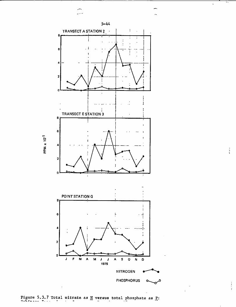
5-44

POINT STATION Gts

J F M A M J J A S O N D

1975

NITROGEN

PHOSPHORUS 0

Figure 5.3.7 Total nitrate as N versus total phosphate as P:

"*7 a x

2

0. CL

-46

4

2

W-ý w I

4.3.2.1 methods and materials three coves representing the

Documents