43610682-final - incentiving no-rush delivery in
TRANSCRIPT
Incentivizing No-Rush Delivery in Omnichannel Retail by
Alison M Heuser Bachelor of Science, Chemical Engineering, Massachusetts Institute of Technology
and
Tabjeel Ashraf Bachelor of Science, Civil Engineering, University of Engineering & Technology
Master of Science, Civil Engineering, University of Engineering & Technology
Master of Project Management, CIIT
SUBMITTED TO THE PROGRAM IN SUPPLY CHAIN MANAGEMENT
IN PARTIAL FULFILLMENT OF THE REQUIREMENTS FOR THE DEGREE OF
MASTER OF APPLIED SCIENCE IN SUPPLY CHAIN MANAGEMENT
AT THE
MASSACHUSETTS INSTITUTE OF TECHNOLOGY
JUNE 2019
© 2019 Alison M Heuser and Tabjeel Ashraf. All rights reserved.
The authors hereby grant to MIT permission to reproduce and to distribute publicly paper and electronic copies of this capstone document in whole or in part in any medium now known or hereafter created.
Signature of Author: ____________________________________________________________
Department of Supply Chain Management May 10, 2019
Signature of Author: ____________________________________________________________ Department of Supply Chain Management
May 10, 2019 Certified by: ___________________________________________________________________
Dr. Eva Ponce Executive Director, MITx MicroMasters in Supply Chain Management
Capstone Advisor Certified by: ___________________________________________________________________
Dr. Sina Golara Postdoctoral Associate Capstone Co-Advisor
Accepted by: __________________________________________________________________ Dr. Yossi Sheffi
Director, Center for Transportation and Logistics Elisha Gray II Professor of Engineering Systems Professor, Civil and Environmental Engineering

2

3
Incentivizing No-Rush Delivery in Omnichannel Retail by
Alison M Heuser
and
Tabjeel Ashraf
Submitted to the Program in Supply Chain Management on May 10, 2019 in Partial Fulfillment of the
Requirements for the Degree of Master of Applied Science in Supply Chain Management
ABSTRACT
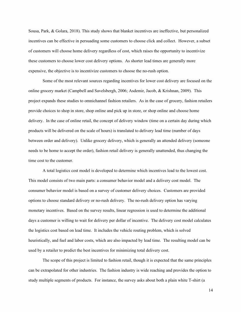
E-commerce sales have grown exponentially since the introduction of the smart phone in 2007 and the trend is expected to continue. As retailers enter e-commerce, the pressure to provide more and faster delivery options to the customer is increasing. The resulting complexity and increased delivery speeds are often expensive. Providing incentives to influence customers to choose no-rush delivery is one method by which retailers can seek to lower these logistics costs. Previous studies have demonstrated that monetary incentives can influence behavior; many researchers have studied logistics costs models. This study focuses on the fast fashion industry and combines research of consumer behavior with a logistics cost model to determine the effectiveness of incentives to drive cost savings. Customers were surveyed for lead time decisions in the presence of varied monetary incentives to determine the impact of the incentive on consumer behavior. The customers were asked about both basic items and trendy items to differentiate behavior between product categories. Linear regression of this data showed that retailers need to provide an incentive of $1.18 per day of extra lead time to a customer purchasing a basic item and $1.14 per day of extra lead time to a customer purchasing a trendy item. These incentives were used as an input cost to a delivery cost model. This model used the vehicle routing problem to estimate logistics costs. The model compared the cost of routes with standard shipping to routes that included no-rush packages over one-week. The results showed that it is possible to save an average of 3% to 32% in logistics costs depending on the percentage of customers who opt in to no-rush delivery. This study showed that it is possible to use incentives to influence consumer behavior and that behavior can have an impact on the logistics costs. It is critical to study both consumer behavior and logistics costs together for a retailer to determine the correct incentives to offer.
Capstone Advisor: Dr. Eva Ponce Title: Executive Director, MITx MicroMasters in Supply Chain Management
Capstone Co-Advisor: Dr. Sina Golara Title: Postdoctoral Associate

4
5
ACKNOWLEDGMENTS
There are a number of people without whom this project would not have been possible. We are grateful for the support and encouragement we have received.
We would like to thank our advisors Dr. Eva Ponce and Dr. Sina Golara for their dedication to their project and for their support and guidance along the way. We are grateful to have been part of this wonderful team. Additional thanks to Dr. Ponce for her dedication to the MicroMasters program, which sparked our interest in Supply Chain Management education at MIT.
We would also like to thank all our colleagues at the MIT Center for Transportation and Logistics. Special thank you to Dr. Chris Caplice for creating the MicroMasters program, without which Alison would not know anything at all about supply chains. Thank you to Professor Yossi Sheffi for teaching us that people do not always do what they say they will do in surveys. Thank you to Dr. Bruce Arntzen for his thoughtful and responsive management of the Supply Chain Management Master Program. Dr. Arntzen has ensured every student gets the most out of their experience here and for that we are grateful. Thank you to Dr. Josué Velázquez-Martinez for being spectacular and for his unwavering belief in the Supply Chain Management Blended Master program, without which neither Alison nor Tabjeel would be here. Thank you to all CTL staff. Thank you to our classmates in the Supply Chain Management Class of 2019. It has been a pleasure learning alongside you.
Thank you, Mom and Dad for instilling a life-long love of learning and for always supporting me along the way. Thank you also for not saying “We told you so” too many times when I changed my mind and decided to get my Master’s degree. Thank you and congratulations to my brother, Will and my sister, Kerri who are also graduating this year with Master’s and Bachelor’s degrees respectively. I am proud and honored to share this graduation season with you. Thank you to my extended family for always being there. Special thanks to Samantha Jaeger, my cousin, who is also sharing this graduation season with Will, Kerri, and me. Last and certainly not least, thank you to Lizz and Molly, my Boston family. Your love and support have gotten me through this program and so much more. -Alison
It would not have been possible for me to come and attend this program without the support of my family. I’m very grateful for their love, care, sacrifice, and their unconditional support. Thank you Anees Fatima for everything you have done to support me and our family. Sajeel and Taseel, you are very young, but I know that both of you are very passionate about coming to MIT. You could not join me this spring because of your schools, but I believe you will work hard and make your own ways to MIT. My wish is that one day you will both graduate from OUR school. - Tabjeel

6
7
TABLE OF CONTENTS LIST OF FIGURES ............................................................................................................................... 8 LIST OF TABLES ............................................................................................................................... 10 1. INTRODUCTION ....................................................................................................................... 12 2. LITERATURE REVIEW ............................................................................................................ 16
2.1 Customer Behavior Model ............................................................................................................ 17 2.2 Delivery Cost Model .................................................................................................................... 18
3. DATA AND METHODOLOGY ................................................................................................. 20 3.1 The Consumer Behavior Model .................................................................................................... 20
3.1.1 Survey................................................................................................................................... 22 3.1.2 Analysis of Survey Data ........................................................................................................ 25
3.2 The Delivery Cost Model .............................................................................................................. 25 3.2.1 Solving the Vehicle Routing Problem and Determining Cost ................................................. 25 3.2.2 Calculating No-Rush Savings ................................................................................................ 26
4. RESULTS AND ANALYSIS ....................................................................................................... 28 4.1 The Customer Behavior Model ..................................................................................................... 28
4.1.1 Survey Data .......................................................................................................................... 30 4.1.2 Correlation Tables ................................................................................................................. 32 4.1.3 Sensitivity Analysis ............................................................................................................... 35
4.2 Delivery Cost Model .................................................................................................................... 38 5. DISCUSSION ............................................................................................................................... 41
5.1 Customer Behavior Model ............................................................................................................ 41 5.2 Delivery Cost Model .................................................................................................................... 43 5.3 Combining the Models ................................................................................................................. 46 5.4 Limitations ................................................................................................................................... 47
6. CONCLUSION ............................................................................................................................ 49 6.1 The Consumer Behavior Model .................................................................................................... 49 6.2 The Delivery Cost Model .............................................................................................................. 49 6.3 Insights and Management Recommendations................................................................................ 50 6.4 Future Research ........................................................................................................................... 50
REFERENCES .................................................................................................................................... 51 APPENDIX A: Customer Behavior Survey ........................................................................................ 53 APPENDIX B: Vehicle Routing Heuristics ........................................................................................ 57 APPENDIX C: Survey Respondent Comments .................................................................................. 58 APPENDIX D: Median Route Visualization – Original vs. No-Rush ................................................ 64

8
LIST OF FIGURES
Figure 1. Ecommerce Retail Sales in the United States. (SSSD, 2019) ................................................... 12 Figure 2. Information and Fulfillment Matrix (Bell et al., 2014) ............................................................. 13 Figure 3. Methodology Overview .......................................................................................................... 20 Figure 4. Experimental Section 1. . ....................................................................................................... 23 Figure 5. Experimental Section 2. . ....................................................................................................... 24 Figure 6: Age and Median Income Distribution of Survey Data.............................................................. 30 Figure 7. Consolidated Sensitivity Analysis Results ............................................................................... 35 Figure 8. Basic Sensitivity Analysis ....................................................................................................... 36 Figure 9. Trendy Sensitivity Analysis .................................................................................................... 37 Figure 10. Distribution of Weekly Cost Over 50 Trials .......................................................................... 38 Figure 11. Lead Time vs. Incentive for the Average Consumer .............................................................. 41 Figure 12. Lead Time vs. Incentive for the Average Consumer with Survey Range Displayed ................ 43 Figure 13. 72% No-Rush Day 7 Original Route and No-Rush Route ...................................................... 44 Figure 14. 5% No-Rush Day 1 ............................................................................................................... 46 Figure 15. 80% No-Rush Day 1 ............................................................................................................. 46 Figure D1. 5% No-Rush Day 1 Original Route and No-Rush Route ....................................................... 64 Figure D2. 5% No-Rush Day 2 Original Route and No-Rush Route ....................................................... 64 Figure D3. 5% No-Rush Day 3 Original Route and No-Rush Route ....................................................... 65 Figure D4. 5% No-Rush Day 4 Original Route and No-Rush Route ....................................................... 65 Figure D5. 5% No-Rush Day 5 Original Route and No-Rush Route ....................................................... 66 Figure D6. 5% No-Rush Day 6 Original Route and No-Rush Route ....................................................... 66 Figure D7. 5% No-Rush Day 7 Original Route and No-Rush Route ....................................................... 67 Figure D8. 20% No-Rush Day 1 Original Route and No-Rush Route ..................................................... 68 Figure D9. 20% No-Rush Day 2 Original Route and No-Rush Route ..................................................... 68 Figure D10. 20% No-Rush Day 3 Original Route and No-Rush Route ................................................... 69 Figure D11. 20% No-Rush Day 4 Original Route and No-Rush Route ................................................... 69 Figure D12. 20% No-Rush Day 5 Original Route and No-Rush Route ................................................... 70 Figure D13. 20% No-Rush Day 6 Original Route and No-Rush Route ................................................... 70 Figure D14. 20% No-Rush Day 7 Original Route and No-Rush Route ................................................... 71 Figure D15. 40% No-Rush Day 1 Original Route and No-Rush Route ................................................... 72 Figure D16. 40% No-Rush Day 2 Original Route and No-Rush Route ................................................... 72 Figure D17. 40% No-Rush Day 3 Original Route and No-Rush Route ................................................... 73 Figure D18. 40% No-Rush Day 4 Original Route and No-Rush Route ................................................... 73 Figure D19. 40% No-Rush Day 5 Original Route and No-Rush Route ................................................... 74 Figure D20. 40% No-Rush Day 6 Original Route and No-Rush Route ................................................... 74 Figure D21. 40% No-Rush Day 7 Original Route and No-Rush Route ................................................... 75 Figure D22. 60% No-Rush Day 1 Original Route and No-Rush Route ................................................... 76 Figure D23. 60% No-Rush Day 2 Original Route and No-Rush Route ................................................... 76 Figure D24. 60% No-Rush Day 3 Original Route and No-Rush Route ................................................... 77 Figure D25. 60% No-Rush Day 4 Original Route and No-Rush Route ................................................... 77 Figure D26. 60% No-Rush Day 5 Original Route and No-Rush Route ................................................... 78 Figure D27. 60% No-Rush Day 6 Original Route and No-Rush Route ................................................... 78 Figure D28. 60% No-Rush Day 7 Original Route and No-Rush Route ................................................... 79 Figure D29. 72% No-Rush Day 1 Original Route and No-Rush Route ................................................... 80 Figure D30. 72% No-Rush Day 2 Original Route and No-Rush Route ................................................... 80 Figure D31. 72% No-Rush Day 3 Original Route and No-Rush Route ................................................... 81
9
LIST OF FIGURES (CONTINUED)
Figure D32. 72% No-Rush Day 4 Original Route and No-Rush Route ................................................... 81 Figure D33. 72% No-Rush Day 5 Original Route and No-Rush Route ................................................... 82 Figure D34. 72% No-Rush Day 6 Original Route and No-Rush Route ................................................... 82 Figure D35. 72% No-Rush Day 7 Original Route and No-Rush Route ................................................... 83 Figure D36. 80% No-Rush Day 1 Original Route and No-Rush Route ................................................... 84 Figure D37. 80% No-Rush Day 2 Original Route and No-Rush Route ................................................... 84 Figure D38. 80% No-Rush Day 3 Original Route and No-Rush Route ................................................... 85 Figure D39. 80% No-Rush Day 4 Original Route and No-Rush Route ................................................... 85 Figure D40. 80% No-Rush Day 5 Original Route and No-Rush Route ................................................... 86 Figure D41. 80% No-Rush Day 6 Original Route and No-Rush Route ................................................... 86 Figure D42. 80% No-Rush Day 7 Original Route and No-Rush Route ................................................... 87

10
LIST OF TABLES
Table 1. Parameter Values for Analysis ................................................................................................. 27 Table 2. Result of Linear Regression for Basic and Trendy Survey Results ............................................ 29 Table 3. Summary Statistics of Survey Response Data ........................................................................... 31 Table 4. ANOVA test: Multiple Factors Analysis Results ...................................................................... 31 Table 5. Basic Model Correlation Table ................................................................................................. 33 Table 6. Trendy Model Correlation Table .............................................................................................. 34 Table 7. Weekly Cost Savings Results Over 50 Trials ............................................................................ 38 Table 8. Impact of Parameter Variation on Cost Savings for 72% No-Rush ............................................ 40 Table 9. 72% No-Rush Day 7 Original Route and No-Rush Route ......................................................... 45 Table 10. 72% Route Totals, Cost Savings, and Trucks Needed over 1 Week ......................................... 45 Table 11. 5% No-Rush Day 1 Original Route and No-Rush Route………………………………………43 Table 12. 80% No-Rush Day 1 Original Route and No-Rush Route ....................................................... 46 Table 13. 5% Route Totals, Cost Savings, and Trucks Needed over 1 Week…………………………….43 Table 14. 80% Route Totals, Cost Savings, and Truck s Needed over 1 Week ........................................ 46 Table C1. Survey Respondent Comment for Basic Item ......................................................................... 58 Table C2. Survey Respondent Comments for Trendy Item ..................................................................... 61 Table D1. 5% No-Rush Day 1 Original Route and No-Rush Route ........................................................ 64 Table D2. 5% No-Rush Day 2 Original Route and No-Rush Route ........................................................ 64 Table D3. 5% No-Rush Day 3 Original Route and No-Rush Route ........................................................ 65 Table D4. 5% No-Rush Day 4 Original Route and No-Rush Route ........................................................ 65 Table D5. 5% No-Rush Day 5 Original Route and No-Rush Route ........................................................ 66 Table D6. 5% No-Rush Day 6 Original Route and No-Rush Route ........................................................ 66 Table D7. 5% No-Rush Day 7 Original Route and No-Rush Route ........................................................ 67 Table D8. 5% Route Totals, Cost Savings, and Trucks Needed over 1 Week .......................................... 67 Table D9. 20% No-Rush Day 1 Original Route and No-Rush Route....................................................... 68 Table D10. 20% No-Rush Day 2 Original Route and No-Rush Route ..................................................... 68 Table D11. 20% No-Rush Day 3 Original Route and No-Rush Route ..................................................... 69 Table D12. 20% No-Rush Day 4 Original Route and No-Rush Route ..................................................... 69 Table D13. 20% No-Rush Day 5 Original Route and No-Rush Route ..................................................... 70 Table D14. 20% No-Rush Day 6 Original Route and No-Rush Route ..................................................... 70 Table D15. 20% No-Rush Day 7 Original Route and No-Rush Route ..................................................... 71 Table D16. 20% Route Totals, Cost Savings, and Trucks Needed over 1 Week ...................................... 71 Table D17. 40% No-Rush Day 1 Original Route and No-Rush Route ..................................................... 72 Table D18. 40% No-Rush Day 2 Original Route and No-Rush Route ..................................................... 72 Table D19. 40% No-Rush Day 3 Original Route and No-Rush Route ..................................................... 73 Table D20. 40% No-Rush Day 4 Original Route and No-Rush Route ..................................................... 73 Table D21. 40% No-Rush Day 5 Original Route and No-Rush Route ..................................................... 74 Table D22. 40% No-Rush Day 6 Original Route and No-Rush Route ..................................................... 74 Table D23. 40% No-Rush Day 7 Original Route and No-Rush Route ..................................................... 75 Table D24. 40% Route Totals, Cost Savings, and Trucks Needed over 1 Week ...................................... 75 Table D25. 60% No-Rush Day 1 Original Route and No-Rush Route ..................................................... 76 Table D26. 60% No-Rush Day 2 Original Route and No-Rush Route ..................................................... 76 Table D27. 60% No-Rush Day 3 Original Route and No-Rush Route ..................................................... 77 Table D28. 60% No-Rush Day 4 Original Route and No-Rush Route ..................................................... 77 Table D29. 60% No-Rush Day 5 Original Route and No-Rush Route ..................................................... 78 Table D30. 60% No-Rush Day 6 Original Route and No-Rush Route ..................................................... 78

11
LIST OF TABLES (CONTINUED)
Table D31. 60% No-Rush Day 7 Original Route and No-Rush Route ..................................................... 79 Table D32. 60% Route Totals, Cost Savings, and Trucks Needed over 1 Week ...................................... 79 Table D33. 72% No-Rush Day 1 Original Route and No-Rush Route ..................................................... 80 Table D34. 72% No-Rush Day 2 Original Route and No-Rush Route ..................................................... 80 Table D35. 72% No-Rush Day 3 Original Route and No-Rush Route ..................................................... 81 Table D36. 72% No-Rush Day 4 Original Route and No-Rush Route ..................................................... 81 Table D37. 72% No-Rush Day 5 Original Route and No-Rush Route ..................................................... 82 Table D38. 72% No-Rush Day 6 Original Route and No-Rush Route ..................................................... 82 Table D39. 72% No-Rush Day 7 Original Route and No-Rush Route ..................................................... 83 Table D40. 72% Route Totals, Cost Savings, and Trucks Needed over 1 Week ...................................... 83 Table D41. 80% No-Rush Day 1 Original Route and No-Rush Route ..................................................... 84 Table D42. 80% No-Rush Day 2 Original Route and No-Rush Route ..................................................... 84 Table D43. 80% No-Rush Day 3 Original Route and No-Rush Route ..................................................... 85 Table D44. 80% No-Rush Day 4 Original Route and No-Rush Route ..................................................... 85 Table D45. 80% No-Rush Day 5 Original Route and No-Rush Route ..................................................... 86 Table D45. 80% No-Rush Day 6 Original Route and No-Rush Route ..................................................... 86 Table D47. 80% No-Rush Day 7 Original Route and No-Rush Route ..................................................... 87 Table D48. 80% Route Totals, Cost Savings, and Trucks Needed over 1 Week ...................................... 87

12
1. INTRODUCTION
Consumer spending represents 69% of the United States Gross Domestic Product (Amadeo,
2019; Amadeo 2018) and therefore the retail industry is vital to the United States economy. Within the
retail industry, there has been a large shift toward e-commerce. In 2018, e-commerce accounted for 9.6%
of retail sales (SSSD, 2019). Figure 1 shows the evolution of e-commerce retail sales. Customers are
looking for new ways to make purchases, including a mix of online and instore purchasing, at-home
delivery, and instore pickup. The iPhone was released in 2007; the age of the smartphone added mobile
options to the already growing range of e-commerce options. Figure 1 shows that as a result of the
smartphone, a trend of exponential growth started in 2007. With online retail growth trends expected to
continue, retailers are moving into the omnichannel space to meet customer needs.
Figure 1. Ecommerce Retail Sales in the United States. (SSSD, 2019)
As omnichannel businesses expand and new delivery and pickup options are introduced,
companies are pressured to provide many options while maintaining positive customer experiences and
meeting profit goals. Bell, Gallino, and Moreno (2014) in their article “How to Win in an Omnichannel
World” describe the options available to customers and the methods by which companies can succeed
0.0%
2.0%
4.0%
6.0%
8.0%
10.0%
12.0%
-
100
200
300
400
500
600
2000
2001
2002
2003
2004
2005
2006
2007
2008
2009
2010
2011
2012
2013
2014
2015
2016
2017
2018
Billi
ons o
f Dol
lars
E-Commerce Retail Sales E-Commerce as Percentage of Total Retail Sales

13
providing multiple options. Figure 2 shows their information and fulfillment matrix. The options include
purchasing direct from a brick and mortar store (traditional retail), purchasing online and picking up in
store (shopping and delivery hybrid, sometimes called “click and collect”), and purchasing online for
delivery – with multiple lead time options (pure-play E-Commerce). These channels can be blurred: a
customer intending to make an instore purchase may purchase online through a mobile app from in the
store (online retail plus showrooms), while a customer intending to make an online purchase may visit the
store to try on clothing and ultimately complete the purchase instore (traditional retail).
Figure 2. Information and Fulfillment Matrix (Bell et al., 2014)
Additional options add complexity and cost. While transaction costs are higher in a brick and mortar
store than online, delivery costs, especially last mile delivery, represent a large cost associated with online
shopping. Delivery costs also provide the greatest opportunity for cost savings.
The goal of this project is to determine incentives that persuade customers to choose longer
shipping lead times (no-rush shipping options) and decrease the total cost of delivery. Previous research
focuses on incentivizing online shoppers to choose click and collect over home delivery (Rabinovich,
14
Sousa, Park, & Golara, 2018). This study shows that blanket incentives are ineffective, but personalized
incentives can be effective in persuading some customers to choose click and collect. However, a subset
of customers will choose home delivery regardless of cost, which raises the opportunity to incentivize
these customers to choose lower cost delivery options. As shorter lead times are generally more
expensive, the objective is to incentivize customers to choose the no-rush option.
Some of the most relevant sources regarding incentives for lower cost delivery are focused on the
online grocery market (Campbell and Savelsbergh, 2006; Asdemir, Jacob, & Krishnan, 2009). This
project expands these studies to omnichannel fashion retailers. As in the case of grocery, fashion retailers
provide choices to shop in store, shop online and pick up in store, or shop online and choose home
delivery. In the case of online retail, the concept of delivery window (time on a certain day during which
products will be delivered on the scale of hours) is translated to delivery lead time (number of days
between order and delivery). Unlike grocery delivery, which is generally an attended delivery (someone
needs to be home to accept the order), fashion retail delivery is generally unattended, thus changing the
time cost to the customer.
A total logistics cost model is developed to determine which incentives lead to the lowest cost.
This model consists of two main parts: a consumer behavior model and a delivery cost model. The
consumer behavior model is based on a survey of customer delivery choices. Customers are provided
options to choose standard delivery or no-rush delivery. The no-rush delivery option has varying
monetary incentives. Based on the survey results, linear regression is used to determine the additional
days a customer is willing to wait for delivery per dollar of incentive. The delivery cost model calculates
the logistics cost based on lead time. It includes the vehicle routing problem, which is solved
heuristically, and fuel and labor costs, which are also impacted by lead time. The resulting model can be
used by a retailer to predict the best incentives for minimizing total delivery cost.
The scope of this project is limited to fashion retail, though it is expected that the same principles
can be extrapolated for other industries. The fashion industry is wide reaching and provides the option to
study multiple segments of products. For instance, the survey asks about both a plain white T-shirt (a

15
basic product) and the latest trending item (a luxury product). This information provides data to
determine whether product segmentation influences the likelihood a customer is willing to choose a no-
rush delivery option, and by how much.

16
2. LITERATURE REVIEW
Home deliveries pose an enormous logistical challenge to retailers due to highly variable costs
and uncertainty in demand, among other factors. Rabinovich et al. (2018) studies incentives in online
grocery to influence customers to choose click and collect (order online and pick up in store) over home
delivery options. The study observes that eliminating the order cost associated with click and collect
increases the revenue. However, the cost increases associated with increased order fulfillment and the
loss of revenue from the order fees outweighs the increased revenue associated with eliminating order
fees. This study concludes that targeted incentives are the most profitable. However, regardless of the
incentive, there is a subset of customers who will choose home delivery options. Based on this
observation, incentivizing customers to choose the lower cost click and collect option is not the only way
to minimize cost. Options in home delivery also provide an opportunity for cost minimization.
Other studies look at options for cost minimization in delivery. Campbell and Savelsbergh
(2005) look at the routing and scheduling problem posed by home delivery in online grocery. The
company decides which orders to accept and reject and sets time slots for accepted deliveries in order to
maximize profits. However, Campbell and Savelsbergh (2006) and Asdemir et al. (2009) note that
customers like choices in delivery options. They study dynamic pricing in home delivery options, rather
than limiting delivery choices to cost minimizing options. Prices are assigned to the delivery windows
such that the grocery retailer is cost-indifferent to the customer’s choice. Specifically, prices are
increased as the time horizon between the order placement and the delivery window decreases. Prices are
also decreased as the demand for a particular delivery window decreases. Furthermore, routing efficiency
is considered when setting prices; orders for which deliveries fit efficiently into existing routs are priced
lower than those that do not fit efficiently. They find that dynamic pricing increases profitability but is
complicated to implement. Yang, Strauss, Currie, and Eglese (2013) also consider decreasing the price
for “green” time slots (time slots that would use less fuel based on insertion into an existing route), which
incentivizes customers to choose the more “green” option. Fu and Saito (2018) find that customers do not
17
need a financial incentive to choose a more “green” option, but rather are inclined to choose the option
marked as “green” absent of incentive.
Campbell and Savelsbergh (2006) also study the option of charging less for longer delivery
windows. They conclude that this option is easier to implement than the dynamic pricing option and
increases profitability. Agatz, Campbell, Fleischman, van Nunen, and Savelsbergh (2013) also conclude
that wider delivery windows are less expensive to the retailer as they provide more flexibility and
therefore more opportunities for cost minimization through routing efficiency. This widening of delivery
windows is specifically studied for attended deliveries, where the customer needs to be present to receive
the order. The downside to a wider delivery window to the customer is time cost associated with The
possibility of waiting longer for the delivery.
This work, mainly in the online grocery market, is expanded to consider the effects of incentives
in the fashion retail industry. The concept of delivery window (time on a certain day during which
groceries will be delivered on the scale of hours) is translated to delivery lead time (number of days
between order and delivery). Unlike grocery delivery which is generally an attended delivery (someone
needs to be home to accept the order), fashion retail delivery is generally unattended, posing a lower time
cost to the customer.
2.1 Customer Behavior Model
In order to determine how incentives impact customers, this project draws on a number of
previous studies. Chintagunta, Chu, and Cebollada (2009) consider consumers to be motivated by a
desire to minimize transaction costs. Chintagunta et al. (2009) consider factors including transportation
costs, psychic costs, adjustment cost due to product unavailability, basket delivery costs, and waiting
costs. The goal of this project is to offer incentives that offset the waiting costs to the customer, thereby
allowing them to choose a less expensive delivery option. Chintagunta et al. (2009) provides a model on
which we can build to accomplish this. (In this particular study, in store shopping time, in store search
costs, and the physical cost of picking items are considered. As these are not applicable to customers

18
choosing home delivery, they will not be considered in the model for this project. Chintagunta et al.
(2009) also consider the cost of not verifying the quality of perishable goods before checking out; this is
not relevant to online retail.)
It is expected that price will have a large impact on customer behavior. Lewis, Singh, and Fay
(2006) cite a study by Jupiter Communications that concludes 60% of online shoppers choose to
discontinue a purchase at the time when shipping fees are added and cite an Ernst and Young study that
shows over half of online shopping customers list shipping fees as their main complaint about online
shopping. Lewis et al. (2006) conclude that free shipping increases order frequency and decreases order
size, policies that waive fees for larger orders increase order size, and customer behavior is impacted
more by the cost of shipping than the price of the merchandise. On the other hand, Unni, Nair, and
Gunasekar (2015) conclude that delivery time windows play a large role in customer satisfaction. As
delivery lead time and price trade off with each other, it is expected that providing monetary incentives
can maintain customer satisfaction with increased delivery lead times.
2.2 Delivery Cost Model
Lewis et al. (2006) conclude that free shipping promotions increase demand and revenue, but do
not increase profit due to the increased cost of shipping. This finding reinforces the idea that the cost of
shipping and delivery must be minimized in order for delivery to be profitable, especially if the customer
is motivated by saving on shipping fees. The incentives must correlate with cost savings to the retailer,
raising the need to determine the impact of increased lead time on delivery cost. A delivery cost model is
determined including delivery labor and fuel (Galante, Lopez, & Monroe, 2013). Vehicle routing is
calculated to determine the fuel and labor cost associated with the actual delivery trip.
The Vehicle Routing Problem, sometimes described as the Traveling Salesman Problem,
describes a situation in which an entity needs to make a number of stops at pre-defined nodes. The goal is
to find the shortest route that includes all of the nodes. The Vehicle Routing Problem has been around for
decades and a lot of work has been carried out to solve this problem. The VRP requires long computation

19
time for an exact solution and therefore many heuristics have been developed to solve VRPs. Clark and
Write (1962) in their famous paper specify the computational algorithm to find the minimum overall
distance for a network. The algorithm uses the savings concept where nodes are joined in such a way that
maximum savings are captured, and routes are formulated to come up with optimal or near optimal
solution. Fisher and Jaikumar (1981) identify generalized assignment heuristics to come up with
minimum travel time for simple scenario.
Parragh, Doerner, and Hartl (2008) argue to incorporate real life constraints into the model and
adjust the simple VRP according to the need. The vehicle routing problem is one of the highest studied
areas in supply chain management and many variants have been considered including capacitated VRP,
mixed Depot VRP, and VRP with pick and delivery. Sharma and Yadav (2018) attempt to review recently
published work in their paper regarding VRP and its variants. They screen 117 papers and conclude that
61 papers focused on VRP with pick and delivery. As recent research has focused on hybrid of heuristics
and algorithms, they have argued that further work can be done to amalgamate of exact and Heuristics
algorithms.
As the customers define the nodes and the required timing of delivery, this project incorporates
the customer behavior into the routing problem to determine the final cost of delivery to the retailer. This
amalgamation of factors into the VRP is consistent with the recommendations of Sharma and Yadav
(2018). Berbeglia, Cordeau, and Laport (2009) compile the work done in dynamic pick and delivery
problem where input data is not known with certainty. Berbeglia et al. (2009) argue for the importance of
different scenarios to solve VRP considering different waiting strategies and real-life assumptions. These
findings are aligned with the approach of this project where assumptions are made for input data and
varying scenarios are considered to provide insight on the impact of customer behavior on vehicle
routing.

20
3. DATA AND METHODOLOGY
A model was developed to determine how to reduce the total logistics cost. The logistics cost
includes the incentive costs and shipping costs (including fuel and labor), as determined by the delivery
cost model. The customer behavior model provides data on the cost of incentive for additional lead time.
The delivery cost model provides data on the cost savings for additional lead time. Figure 3 shows an
overview of the methodology.
Figure 3. Methodology Overview
3.1 The Consumer Behavior Model
The consumer behavior model is used to determine how incentives impact the delivery lead time
option chosen by the consumer at the time of checkout for online retail. Data for this model was collected
via a consumer survey. The survey provided an online retail narrative and a set of delivery choices, from
which the respondents were asked to choose. The incentives offered and the narrative were varied while
the choices remained the same. Basic demographic information including zip code, age, sex, and nature
of employment was collected. From this data, a mathematical model was proposed that predicts a
delivery lead time choice based on consumer and incentive information.

21
!". 1&'()*+, = ./0 + 20/3 + 23/4 + 24/5 + 25/6 + 26/7 + 80/9 + 83/: + 84/; + <0/0= + <3/00 + >0/03 + >3/04 + >4/05 + ?/06 + @/07 + A/09 + B
!". 2&'DEFGHI = ./0 + 20/3 + 23/4 + 24/5 + 25/6 + 26/7 + 80/9 + 83/: + 84/; + <0/0= +<3/00 + >0/03 + >3/04 + >4/05 + ?/06 + @/07 + A/09 + B
JℎLML:
&' = OℎPQLRSLTUVWXL(UTZQ) /0 = WROLRVW\L($)
/3 = UTWSZQℎP^^LM{0,1} /4 = JLLcSZQℎP^^LM{0,1} /5 = dWJLLcSZQℎP^^LM{0,1} /6 = XPRVℎSZQℎP^^LM{0,1} /7 = ZLTMSZQℎP^^LM{0,1}
/9 = eQeTSJTWVVWXL: 2PMfLJLMUTZQ{0,1} /: = eQeTSJTWVVWXL: 3 − 6UTZQ{0,1}
/; = eQeTSJTWVVWXL: 7PMXPMLUTZQ{0,1} /0= = fLXTSL{0,1} /00 = XTSL{0,1}
/03 = LX^SPZLUfeSSVWXL{0,1} /04 = LX^SPZLU^TMV − VWXL{0,1}
/05 = QVeULRV{0,1} /06 = UL^LRULRVQ{0,1}
/07 = TkL /09 = XLUWTRℎPeQLℎPSUWROPXL($)
Using this model, values are determined for the number of days a customer is willing to wait per
extra dollar of incentive (α), and the number of days a customer is willing to wait based on their shopping
frequency (20 for daily shoppers, 23 for weekly shoppers, 24 for biweekly shoppers, 25 for monthly
shoppers, and 26 for yearly shoppers), usual wait time (80 for usual wait times of 2 or fewer days, 83 for
usual wait times of 3-6 days, and 84 for usual wait times of 7 or more days), gender (<0 for female
shoppers and <3 for male shoppers), employment status (>0 for full-time employees, >3 for part-time
employees, and >4 for students), whether the customer has dependents (?), age (@), and median household
income (A) – determined by the zip code in which the customer resides. Note that respondents who have
never shopped before will have a value of 0 for /3l7 and /9l:. The impact of having never shopped
online is incorporated into the base model. Similarly, respondents who identify their employment status
as something other than full-time, part-time, or student will have a value of 0 for /03l05. The impact of

22
other employment is incorporated into the base model. Finally, respondents who identify as neither male
nor female will have a value of 0 for /0=l00 and the impact of identifying with another gender is
considered by the base model.
Correlation analysis was run to understand the dataset better for both the models. A model was
formulated in python to calculate the correlation of all the features in the dataset (including target) to
identify which pair of features have the highest correlation among the dataset.
To ascertain the most important independent variables sensitivity analysis was carried out using
Monte Carlo Simulation technique. This analysis included a procedure of changing values of one
independent variable at a time and keeping all other independent variables constant. This procedure was
repeated for all the independent variables and an assessment was made to determine the variable which
affects the output the most. A probabilistic model was developed using Monte Carlo simulation procedure
to carry out sensitivity analysis in stochastic environment. The model used regression analysis for both
the trendy and basic models in Microsoft Excel. After checking the validity of the model in a
deterministic environment, uncertainty in inputs was introduced. The lead time was calculated with
100,000 iterations for each model using the Monte Carlo simulator to differ input values.
3.1.1 Survey
The survey sought to determine the impact of a given incentive on the customer delivery choice.
The survey consisted of 4 parts: pre-questions, incentive and delivery choice of a basic item (plain white
shirt), incentive and delivery choice of a trendy item, and basic demographic information. The pre-
questions asked the respondents to answer questions about their current online shopping habits: “How
often do you shop online?” and “How long do you usually wait for delivery?” These questions were
asked before the experimental questions to avoid any bias caused by delivery lead time selection in the
experimental sections. The delivery windows for these questions were informed by a sampling of
existing online and omnichannel retailers including Vineyard Vines, J. Crew, Lululemon, American Eagle
Outfitters, Nordstrom, Macy’s, and Zara (American Eagle Outfitters 2018; Fees and Timing | lululemon
23
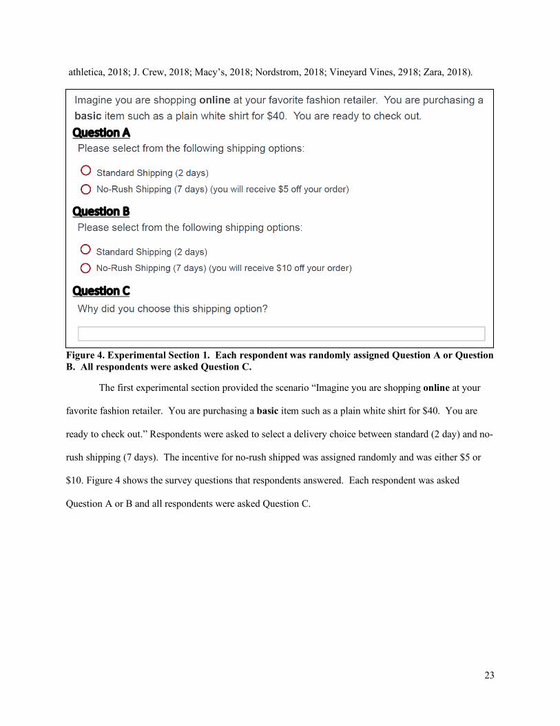
athletica, 2018; J. Crew, 2018; Macy’s, 2018; Nordstrom, 2018; Vineyard Vines, 2918; Zara, 2018).
Figure 4. Experimental Section 1. Each respondent was randomly assigned Question A or Question B. All respondents were asked Question C.
The first experimental section provided the scenario “Imagine you are shopping online at your
favorite fashion retailer. You are purchasing a basic item such as a plain white shirt for $40. You are
ready to check out.” Respondents were asked to select a delivery choice between standard (2 day) and no-
rush shipping (7 days). The incentive for no-rush shipped was assigned randomly and was either $5 or
$10. Figure 4 shows the survey questions that respondents answered. Each respondent was asked
Question A or B and all respondents were asked Question C.
Question A
Question B
Question C
24
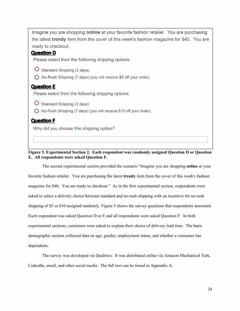
Figure 5. Experimental Section 2. Each respondent was randomly assigned Question D or Question E. All respondents were asked Question F.
The second experimental section provided the scenario “Imagine you are shopping online at your
favorite fashion retailer. You are purchasing the latest trendy item from the cover of this week's fashion
magazine for $40. You are ready to checkout.” As in the first experimental section, respondents were
asked to select a delivery choice between standard and no-rush shipping with an incentive for no-rush
shipping of $5 or $10 assigned randomly. Figure 5 shows the survey questions that respondents answered.
Each respondent was asked Question D or E and all respondents were asked Question F. In both
experimental sections, customers were asked to explain their choice of delivery lead time. The basic
demographic section collected data on age, gender, employment status, and whether a consumer has
dependents.
The survey was developed via Qualtrics. It was distributed online via Amazon Mechanical Turk,
LinkedIn, email, and other social media. The full text can be found in Appendix A.
Question D
Question E
Question F

25
3.1.2 Analysis of Survey Data
Descriptive analytics were run on the survey results. Respondents who did not provide a gender,
age, or valid US zip code were removed. The median income associated with the provided zip code was
determined from census data was included in the results. The uszipcode API for Python was used to look
up the median income data for a given Zip Code.
The data was randomly split into two groups for independent analysis. For the first group, only
the data related to the basic item was considered. For the second group, only the data related to the trendy
item was considered. As each participant was asked about both a basic and a trendy item, the selected
lead times for each of the two questions are expected to be correlated. By splitting the data into two
random and independent groups, the data was analyzed with linear regression without concern for
correlation
The open-ended questions which asked customers to explain their choice of delivery lead time
were considered to gain insight into the customer decisions. The answers to these questions are not
included in the mathematical model.
3.2 The Delivery Cost Model
The delivery cost model assigned a logistics cost to a week’s worth of deliveries with and without
a no-rush shipping option and calculated the cost savings. As we assume the majority of the logistics
costs comes for the last-mile delivery, the model assigned only costs associated with final delivery to the
customer. In order to calculate these costs, the model used the vehicle routing problems (VRPs) with
estimated fuel and labor costs.
3.2.1 Solving the Vehicle Routing Problem and Determining Cost
For vehicle routing, the assumption was made that one truck carried a set of packages from a
single distribution center over a 7-day period. The model is designed to accept a list of packages with
point locations around the origin (distribution center) and day of delivery (1-7). The route for each day
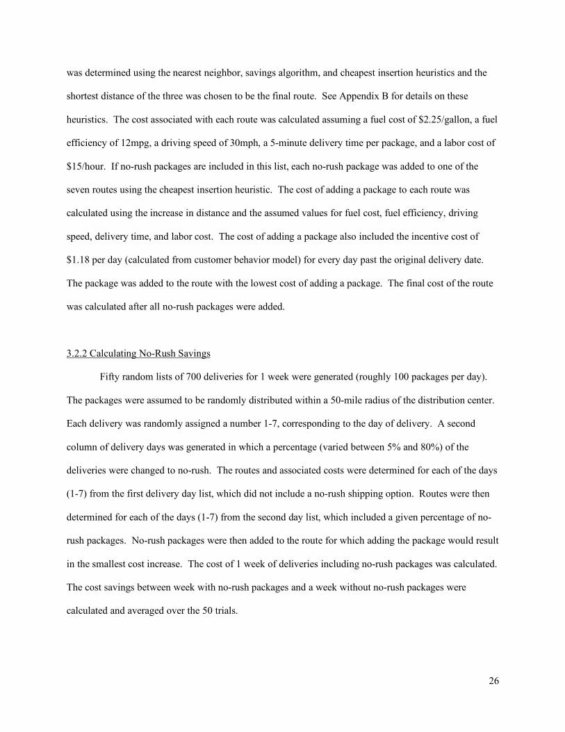
26
was determined using the nearest neighbor, savings algorithm, and cheapest insertion heuristics and the
shortest distance of the three was chosen to be the final route. See Appendix B for details on these
heuristics. The cost associated with each route was calculated assuming a fuel cost of $2.25/gallon, a fuel
efficiency of 12mpg, a driving speed of 30mph, a 5-minute delivery time per package, and a labor cost of
$15/hour. If no-rush packages are included in this list, each no-rush package was added to one of the
seven routes using the cheapest insertion heuristic. The cost of adding a package to each route was
calculated using the increase in distance and the assumed values for fuel cost, fuel efficiency, driving
speed, delivery time, and labor cost. The cost of adding a package also included the incentive cost of
$1.18 per day (calculated from customer behavior model) for every day past the original delivery date.
The package was added to the route with the lowest cost of adding a package. The final cost of the route
was calculated after all no-rush packages were added.
3.2.2 Calculating No-Rush Savings
Fifty random lists of 700 deliveries for 1 week were generated (roughly 100 packages per day).
The packages were assumed to be randomly distributed within a 50-mile radius of the distribution center.
Each delivery was randomly assigned a number 1-7, corresponding to the day of delivery. A second
column of delivery days was generated in which a percentage (varied between 5% and 80%) of the
deliveries were changed to no-rush. The routes and associated costs were determined for each of the days
(1-7) from the first delivery day list, which did not include a no-rush shipping option. Routes were then
determined for each of the days (1-7) from the second day list, which included a given percentage of no-
rush packages. No-rush packages were then added to the route for which adding the package would result
in the smallest cost increase. The cost of 1 week of deliveries including no-rush packages was calculated.
The cost savings between week with no-rush packages and a week without no-rush packages were
calculated and averaged over the 50 trials.

27
The same procedure was followed using varying values for fuel cost, fuel efficiency, driving
speed, delivery time per package, and labor cost. Using 72% no-rush, 10 trials were run as shown in
Table 1 to demonstrate the effect on each parameter on cost savings.
Table 1. Parameter Values for Analysis Trial Variable 1 2 3 4 5 6 7 8 9 10 Fuel Efficiency (MPG) 6 24 12 12 12 12 12 12 12 12 Fuel Cost ($) $2.25 $2.25 $1.13 $4.50 $2.25 $2.25 $2.25 $2.25 $2.25 $2.25 Labor Cost ($) $15.00 $15.00 $15.00 $15.00 $7.50 $30.00 $15.00 $15.00 $15.00 $15.00 Speed (mph) 30 30 30 30 30 30 15 60 30 30 Package Drop-off Speed (mins) 5 5 5 5 5 5 5 5 2.5 1
28
4. RESULTS AND ANALYSIS
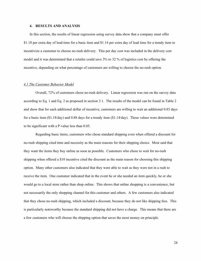
In this section, the results of linear regression using survey data show that a company must offer
$1.18 per extra day of lead time for a basic item and $1.14 per extra day of lead time for a trendy item to
incentivize a customer to choose no-rush delivery. This per day cost was included in the delivery cost
model and it was determined that a retailer could save 3% to 32 % of logistics cost by offering the
incentive, depending on what percentage of customers are willing to choose the no-rush option.
4.1 The Customer Behavior Model
Overall, 72% of customers chose no-rush delivery. Linear regression was run on the survey data
according to Eq. 1 and Eq. 2 as proposed in section 3.1. The results of the model can be found in Table 2
and show that for each additional dollar of incentive, customers are willing to wait an additional 0.85 days
for a basic item ($1.18/day) and 0.88 days for a trendy item ($1.14/day). These values were determined
to be significant with a P-value less than 0.05.
Regarding basic items, customers who chose standard shipping even when offered a discount for
no-rush shipping cited time and necessity as the main reasons for their shipping choice. Most said that
they want the items they buy online as soon as possible. Customers who chose to wait for no-rush
shipping when offered a $10 incentive cited the discount as the main reason for choosing this shipping
option. Many other customers also indicated that they were able to wait as they were not in a rush to
receive the item. One customer indicated that in the event he or she needed an item quickly, he or she
would go to a local store rather than shop online. This shows that online shopping is a convenience, but
not necessarily the only shopping channel for this customer and others. A few customers also indicated
that they chose no-rush shipping, which included a discount, because they do not like shipping fees. This
is particularly noteworthy because the standard shipping did not have a charge. This means that there are
a few customers who will choose the shipping option that saves the most money on principle.

29
Table 2. Result of Linear Regression for Basic and Trendy Survey Results Basic Trendy Coefficient P-Value Coefficient P-Value
α (days/$) 0.85 1.125E-06 0.88 1.655E-07 β1 (days for daily shopper) -1.32 0.146 -1.06 0.244 β2 (days for weekly shopper) -1.27 0.143 -0.87 0.186 β3 (days for biweekly shopper) -0.09 0.915 -0.19 0.725 β4 (days for monthly shopper) -1.28 0.083 -0.08 0.871 β5 (days for yearly shopper) -0.84 0.229 -0.01 0.989
γ1 (days for usual wait time of 2 days or fewer) -1.76 0.115 -1.44 0.041 γ2 (days for usual wait time of 3-6 days) -1.48 0.139 -0.15 0.793
γ3 (days for usual wait time of 7 or more days) -1.56 0.218 -0.62 0.291 δ1 (days for female) 0.15 0.873 -0.80 0.161 δ2 (days for male) -1.31 0.135 -1.41 0.009
ζ1 (days for full-time employees) 0.58 0.353 1.46 0.091 ζ2 (days for part-time employees) 0.62 0.414 1.81 0.069
ζ3 (days for students) 2.12 0.031 1.87 0.133 η (days for dependents) -1.35 0.008 0.72 0.205
θ (days/year) 0.02 0.333 -0.02 0.458 κ (days/$) 2.08E-05 0.047 5.81E-06 0.531 ε (intercept) -1.16 0.496 -2.21 0.025
R2 0.67 0.67 For trendy items, customers who chose standard shipping even when offered a discount for no-
rush shipping cited time as the main reason for their shipping choice. Many customers indicated that a
trendy item is important to have quickly. Some expressed concerns for stockouts and missing trends,
while other indicated wanting to wear the item faster. Customers who chose no-rush shipping (when
offered a $10 incentive) cited the discount for the main reason for choosing this shipping option.
It is important to note that no comments were offered from customers who chose no-rush
shipping when offered a $5 incentive for either basic or trendy items. The full text of the comments can
be found in Appendix B.
30
4.1.1 Survey Data
The survey received 219 responses. Eighty-seven of the respondents were male and 96 were
female. No respondents identified with a gender other than male or female. Thirty-six respondents did
not supply gender. Unfinished responses were removed leaving 155 respondents, 72 of which were male,
82 of which were female, and 1 did not supply gender. The response without a specified gender was
eliminated for a total of 154 responses – 72 male and 82 female. The ages of the respondents ranged from
19 to 66 with an average age of 35 and a median age of 33. Six respondents did not provide age and were
removed resulting in a total of 148 responses – 67 male and 81 female. Thirty-five respondents did not
provide valid US zip codes (used for median income lookup) and were eliminated for a total of 113
responses – 49 male (43.4%) and 64 female (56.6%) with an age range of 19 to 66, average age of 36, and
median age of 34.
The data was randomly split into 2 groups – one was analyzed based on the response to the basic
item section and the other was analyzed based on the response to the trendy item section. This allowed
for independent regression models to be run on each group as we expected the responses to the two
sections to be correlated for any given respondent. The basic item data included 52 responses – 21 male
and 31 female with an age range of 24 to 66, an average age of 37, and a median age of 36. The trendy
item data included 51 responses – 25 male and 26 female with an age range of 19 to 60, an average age of
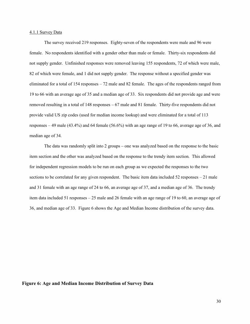
36, and median age of 33. Figure 6 shows the Age and Median Income distribution of the survey data.
010203040506070
Age Distribution
Full Data Basic Data Trendy Data
$-
$50,000.00
$100,000.00
$150,000.00
$200,000.00
$250,000.00
Median Income Distribution
Basic Data Trendy Data
Figure 6: Age and Median Income Distribution of Survey Data

31
Table 3 reports summary statistics on the survey data including number of respondents characterized by
gender and Age and Median Income summary statistics.
Table 3. Summary Statistics of Survey Response Data Full Data Basic Data Trendy Data Number of Respondents 113 52 51 Male 49 21 25 Female 64 31 26
Age
Mean 34 37 35 Median 33 36 33 Min 19 24 19 Max 58 66 60 Lower Quartile 28 28 28 Upper Quartile 38 45 40 Mode 30 32 22
Median Income
Mean $ 53,248 $ 52,959 Median $ 43,380 $ 50,000 Min $ 17,483 $ 17,253 Max $ 116,347 $ 220,583 Lower Quartile $ 38,643 $ 39,952 Upper Quartile $ 62,183 $ 62,618 Mode $ 101,634 $ 41,737
To minimize the bias and ensure the effectiveness of the data split, a study was carried out to
show there was no significant difference between the two data sets. A two-way ANOVA test with
replication was used and the results are given in Table 4.
Table 4. ANOVA test: Multiple Factors Analysis Results
Source of Variation SS df MS F P-value F crit Sample 59030673 1 59030672.6 1.629189729 0.201970494 3.846337168
Columns 297311788302 17 17488928724 482.6775944 0 1.628126381
Interaction 1004142687 17 59067216.86 1.630198315 0.049553912 1.628126381
Within 69132846414 1908 36233148.02
Total 3.67508E+11
1943
32
It is clear that the P value is more than alpha =0.05 (95 % confidence level), and the F value is
less than F Critical; therefore, it was deduced that the means of two (2) groups are statistically equal with
95% reliability.
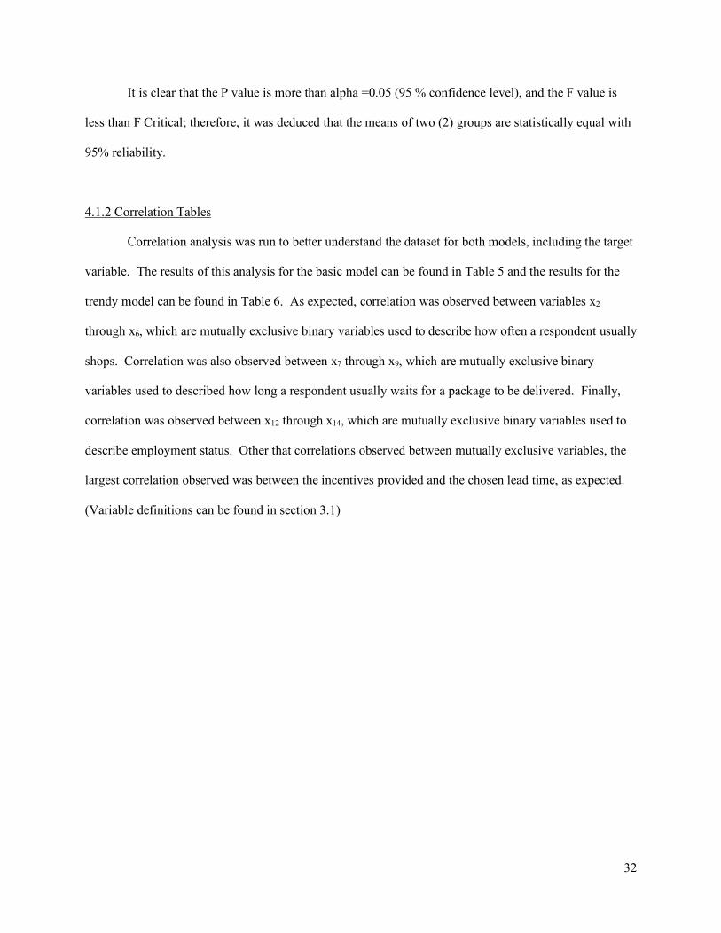
4.1.2 Correlation Tables
Correlation analysis was run to better understand the dataset for both models, including the target
variable. The results of this analysis for the basic model can be found in Table 5 and the results for the
trendy model can be found in Table 6. As expected, correlation was observed between variables x2
through x6, which are mutually exclusive binary variables used to describe how often a respondent usually
shops. Correlation was also observed between x7 through x9, which are mutually exclusive binary
variables used to described how long a respondent usually waits for a package to be delivered. Finally,
correlation was observed between x12 through x14, which are mutually exclusive binary variables used to
describe employment status. Other that correlations observed between mutually exclusive variables, the
largest correlation observed was between the incentives provided and the chosen lead time, as expected.
(Variable definitions can be found in section 3.1)

33
Table 5. Basic Model Correlation Table
LT x1 x2 x3 x4 x5 x6 x7 x8 x9 x10 x12 x13 x14 x15 x16 x17 LT 1.00
x1 0.66 1.00
x2 -0.18 -0.12 1.00
x3 0.05 0.13 -0.10 1.00
x4 0.22 0.14 -0.11 -0.14 1.00
x5 -0.18 -0.24 -0.21 -0.26 -0.29 1.00
x6 0.07 0.11 -0.19 -0.24 -0.26 -0.49 1.00
x7 -0.02 -0.01 -0.12 -0.15 0.14 -0.09 0.18 1.00
x8 -0.11 -0.07 0.00 0.21 -0.03 0.14 -0.19 -0.74 1.00
x9 0.16 0.10 0.19 -0.10 -0.11 -0.06 0.12 -0.12 -0.50 1.00
x10 0.11 -0.17 -0.06 -0.07 0.21 0.19 -0.22 0.03 0.07 -0.06 1.00
x12 -0.03 0.04 -0.03 -0.04 0.24 -0.17 0.01 -0.05 -0.07 0.11 0.06 1.00
x13 -0.02 -0.18 0.08 0.01 -0.17 0.14 -0.05 -0.18 0.25 -0.12 0.24 -0.48 1.00
x14 0.02 -0.09 -0.09 0.09 -0.13 0.04 0.07 0.04 -0.11 0.15 -0.40 -0.37 -0.14 1.00
x15 -0.30 -0.20 0.11 0.08 0.24 -0.08 -0.25 0.06 0.02 -0.18 0.21 0.22 -0.05 -0.10 1.00
x16 0.08 -0.03 0.07 0.05 0.04 0.08 -0.17 0.05 0.09 -0.19 0.34 -0.22 0.21 -0.18 0.14 1.00
x17 0.16 0.01 0.07 0.20 -0.02 -0.03 -0.10 0.09 -0.19 0.23 0.03 -0.13 0.07 0.00 0.09 -0.03 1.00 Correlation between incentives and lead time Correlation between variables describing usual shopping frequency Correlation between variables describing variables describing usual wait time for package delivery Correlation between variables describing employment status

34
Table 6. Trendy Model Correlation Table
LT x1 x2 x3 x4 x5 x6 x7 x8 x9 x10 x12 x13 x14 x15 x16 x17 LT 1.00
x1 0.62 1.00
x2 -0.06 0.13 1.00
x3 -0.01 -0.13 -0.08 1.00
x4 -0.12 -0.15 -0.17 -0.13 1.00
x5 -0.01 0.03 -0.26 -0.20 -0.44 1.00
x6 0.17 0.10 -0.17 -0.13 -0.29 -0.44 1.00
x7 -0.19 -0.34 0.18 0.09 0.20 -0.30 -0.03 1.00
x8 0.14 0.28 -0.20 -0.01 -0.12 0.24 -0.02 -0.70 1.00
x9 0.02 0.01 0.07 -0.09 -0.07 0.02 0.06 -0.18 -0.57 1.00
x10 0.20 0.10 -0.01 0.19 -0.03 -0.03 -0.03 -0.01 0.20 -0.26 1.00
x12 0.00 -0.09 -0.17 0.01 0.11 -0.02 0.02 -0.15 0.00 0.17 0.13 1.00
x13 0.08 0.13 0.12 -0.08 -0.17 0.13 -0.02 0.01 0.08 -0.12 0.12 -0.43 1.00
x14 -0.01 -0.18 -0.11 0.17 -0.05 0.07 -0.05 0.13 -0.14 0.04 -0.32 -0.48 -0.11 1.00
x15 -0.26 -0.36 0.02 0.21 0.19 -0.05 -0.26 0.12 0.06 -0.23 0.31 0.23 0.02 -0.17 1.00
x16 0.20 0.21 -0.11 -0.08 -0.07 0.13 0.04 -0.25 0.37 -0.22 0.25 0.04 0.19 -0.33 -0.08 1.00
x17 0.12 0.10 0.19 0.06 0.02 -0.02 -0.16 -0.03 -0.02 0.06 0.08 -0.24 0.12 -0.07 -0.04 -0.07 1.00 Correlation between incentives and lead time Correlation between variables describing usual shopping frequency Correlation between variables describing variables describing usual wait time for package delivery Correlation between variables describing employment status

35
4.1.3 Sensitivity Analysis
A sensitivity analysis was run on the customer behavior model to determine the impact of varying
inputs. Figure 7 shows the consolidated results.
Figure 7. Consolidated Sensitivity Analysis Results
For the basic model, the sensitivity analysis showed that under the incentives, average lead time
comes out to be 1.2 days, which is not a large change in behavior. Regression coefficient sensitivity and
correlation coefficients sensitivity were considered, and the results for the basic model can be seen in
Figure 8. The sensitivity analysis showed that the incentive is the most sensitive input to the lead time.
Furthermore, gender was shown to have a greater effect on the choice of lead time for the basic product
than for the trendy product.
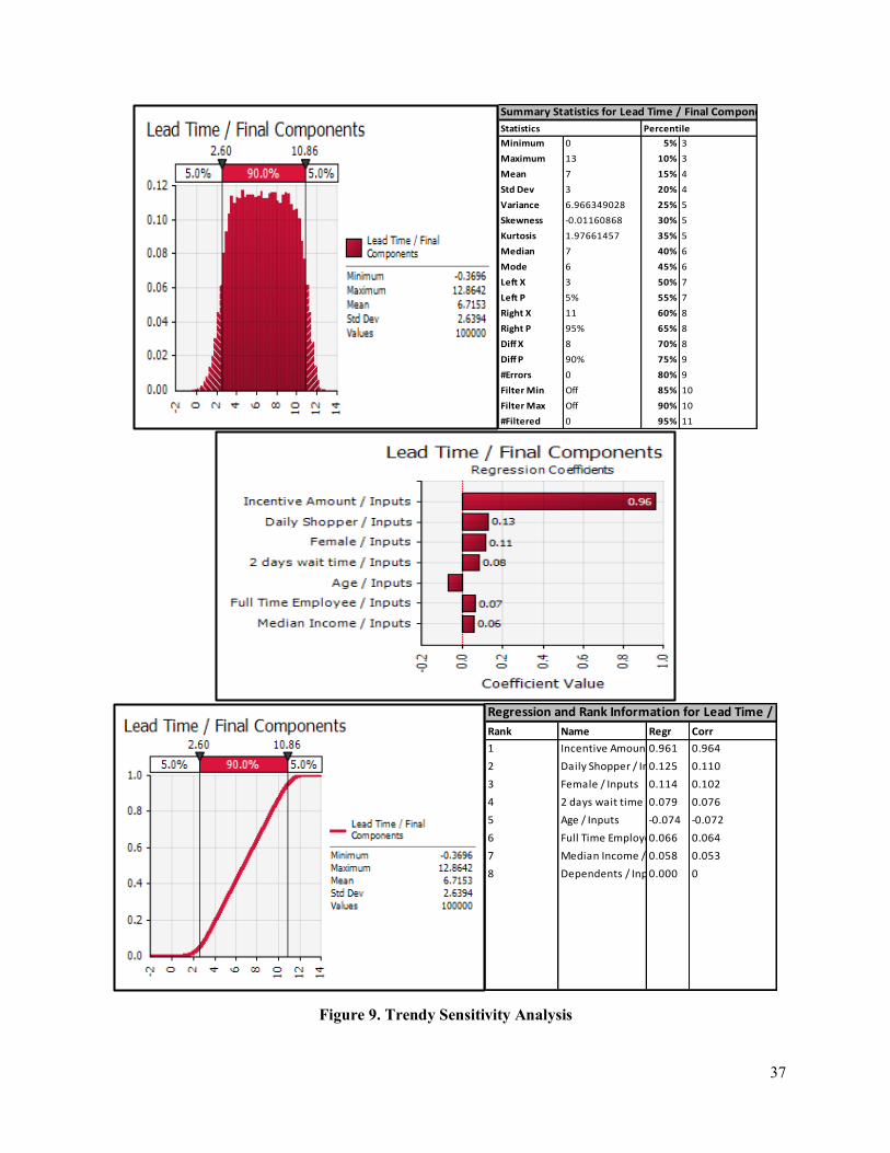
For the trendy model, the sensitivity analysis showed that under the incentives, average lead time
comes to be 7 days, which shows a large change in behavior. The results for the trendy model can be
seen in Figure 9. The sensitivity analysis showed that the incentive is the most sensitive input to the lead
time for the trendy product, as for the basic product. Respondents who shop more often display a greater
response to monetary benefit. Gender has an effect on the choice of lead time for the trendy product, but
to a lesser extent than the effect of gender on lead time choice for the basic product. Age was shown to be
less sensitive than other variables to change in lead time and younger shoppers were more sensitive to
monetary benefits than older shoppers
Rank For H21
Sheet Name Description Trendy Sensitivity Analysis!H21Lead Time / Final ComponentsRegression Coeff.RSqr=0.972
Basic Sensitivity Analysis!H21Lead Time / Final ComponentsRegression Coeff.RSqr=0.961
#1 Trendy Sensitivity Analysis Incentive Amount / Inputs RiskUniform(C3,D3) 0.961 n/a
#2 Trendy Sensitivity Analysis Daily Shopper / Inputs RiskDiscrete({0,1,2,3,4},{0.08,0.14,0.16,0.4,0.22}) 0.125 n/a#3 Trendy Sensitivity Analysis Female / Inputs RiskDiscrete({0,1},{0.57,0.43}) 0.114 n/a
#4 Trendy Sensitivity Analysis 2 days wait time / Inputs RiskDiscrete({0,1,2},{0.15,0.68,0.17}) 0.079 n/a#5 Trendy Sensitivity Analysis Age / Inputs RiskNormal(C18,D18) -0.074 n/a
#6 Trendy Sensitivity Analysis Full Time Employee / Inputs RiskDiscrete({0,1,2},{0.57,0.32,0.11}) 0.066 n/a
#7 Trendy Sensitivity Analysis Median Income / Inputs RiskNormal(C19,D19) 0.058 n/a
- Trendy Sensitivity Analysis Dependents / Inputs RiskDiscrete({1},{0.57}) 0 n/a- Basic Sensitivity Analysis Median Income / Inputs RiskNormal(C19,D19) n/a 0.201
- Basic Sensitivity Analysis Age / Inputs RiskNormal(C18,D18) n/a 0.09- Basic Sensitivity Analysis Dependents / Inputs RiskDiscrete({1},{0.57}) n/a 0
- Basic Sensitivity Analysis Full Time Employee / Inputs RiskDiscrete({0,1,2},{0.57,0.32,0.11}) n/a 0.136
- Basic Sensitivity Analysis Female / Inputs RiskDiscrete({0,1},{0.57,0.43}) n/a 0.266- Basic Sensitivity Analysis 2 days wait time / Inputs RiskDiscrete({0,1,2},{0.15,0.68,0.17}) n/a 0.019
- Basic Sensitivity Analysis Daily Shopper / Inputs RiskDiscrete({0,1,2,3,4},{0.08,0.14,0.16,0.4,0.22}) n/a 0.014- Basic Sensitivity Analysis Incentive Amount / Inputs RiskUniform(C3,D3) n/a 0.91

36
Figure 8. Basic Sensitivity Analysis
Statistics PercentileMinimum -6 5% -3Maximum 10 10% -2Mean 1 15% -2Std Dev 3 20% -1Variance 7.331595397 25% -1Skewness 0.020370469 30% 0Kurtosis 2.17527963 35% 0Median 1 40% 0Mode 0 45% 1Left X -3 50% 1Left P 5% 55% 2Right X 6 60% 2Right P 95% 65% 3Diff X 9 70% 3Diff P 90% 75% 3#Errors 0 80% 4Filter Min Off 85% 4Filter Max Off 90% 5#Filtered 0 95% 6
Summary Statistics for Lead Time / Final Components
Rank Name Regr Corr1 Incentive Amount / Inputs0.910 0.914
2 Female / Inputs 0.266 0.246
3 Median Income / Inputs0.201 0.184
4 Full Time Employee / Inputs0.136 0.097
5 Age / Inputs 0.090 0.083
6 2 days wait time / Inputs0.019 0.015
7 Daily Shopper / Inputs0.014 -0.004
8 Dependents / Inputs0.000 0
Regression and Rank Information for Lead Time / Final Components
37
Figure 9. Trendy Sensitivity Analysis
Statistics PercentileMinimum 0 5% 3Maximum 13 10% 3Mean 7 15% 4Std Dev 3 20% 4Variance 6.966349028 25% 5Skewness -0.01160868 30% 5Kurtosis 1.97661457 35% 5Median 7 40% 6Mode 6 45% 6Left X 3 50% 7Left P 5% 55% 7Right X 11 60% 8Right P 95% 65% 8Diff X 8 70% 8Diff P 90% 75% 9#Errors 0 80% 9Filter Min Off 85% 10Filter Max Off 90% 10#Filtered 0 95% 11
Summary Statistics for Lead Time / Final Components
Rank Name Regr Corr1 Incentive Amount / Inputs0.961 0.9642 Daily Shopper / Inputs0.125 0.1103 Female / Inputs 0.114 0.1024 2 days wait time / Inputs0.079 0.0765 Age / Inputs -0.074 -0.0726 Full Time Employee / Inputs0.066 0.0647 Median Income / Inputs0.058 0.0538 Dependents / Inputs0.000 0
Regression and Rank Information for Lead Time / Final Components

38
4.2 Delivery Cost Model
Over 50 trials of simulated data, using the incentive cost per day as calculated in the customer
behavior model, the average weekly cost savings associated with 5%, 20%, 40%, 60%, 72% and 80% no-
rush packages were calculated. Results can be found in Table 7. These results show the potential for an
average of 3% to 32 % cost savings depending on the percent of customers who choose no-rush delivery.
Table 7. Weekly Cost Savings Results Over 50 Trials Percent No-Rush 5% 20% 40% 60% 72% 80% Mean $ 119.64 $ 321.06 $ 686.12 $ 1,043.24 $ 1,226.81 $ 1,440.00 Median $ 94.88 $ 299.06 $ 641.78 $ 1,024.72 $ 1,207.44 $ 1,441.00 Min $ (88.00) $ 45.38 $ 398.75 $ 784.13 $ 929.51 $ 1,180.15 Max $ 672.19 $ 796.19 $ 1,189.19 $ 1,544.38 $ 1,718.06 $ 1,849.31 Lower Quartile $ 28.19 $ 222.06 $ 587.13 $ 958.97 $ 1,122.00 $ 1,344.06 Upper Quartile $ 153.02 $ 386.87 $ 786.84 $ 1,118.00 $ 1,311.89 $ 1,517.86 Mode $ 64.63 $ 587.13 $ 983.81 Mean (as %) 2.7% 7.2% 15.4% 23.5% 27.7% 32.4%
Figure 10 shows the distribution of cost savings for each percentage of no-rush packages. At 5% no-rush,
it is possible for the cost of delivery with a no-rush option to be more expensive than the cost of delivery
without the no-rush option. Above 5% no-rush, no trials were observed in which the cost of delivery with
a no-rush option was more expensive than the cost of delivery without the no-rush option.
Figure 10. Distribution of Weekly Cost Over 50 Trials

39
The cost associated with each route was calculated assuming a fuel cost of $2.25/gallon, a fuel efficiency
of 12mpg, a driving speed of 30mph, a 5-minute delivery time per package, and a labor cost of $15/hour.
These values are likely to change for different retailers and types of delivery fleets. The results of this
analysis are heavily dependent on these constants; therefore, 10 trials were run varying these parameters
(refer to Table 1 in section 3.2.2). With a no-rush percentage of 72%, the results of these trials can be
found in Table 8. Labor cost and speed have the highest impact on mean cost savings. Labor cost is
based on the amount of time for the delivery route and speed directly impacts time. Higher fuel
efficiency means lower cost savings as fuel is the second largest cost after labor. The time it takes to drop
off a package has no impact on the cost savings. It impacts labor costs; for the same number of packages
in a given week, it takes the same amount of time to delivery regardless of the route. Therefore, no-rush
shipping has no impact on cost savings associated with delivery time per package.

40
Table 8. Impact of Parameter Variation on Cost Savings for 72% No-Rush Trial 1 2 3 4 5 6 7 8 9 10
Trial Description
Fuel Efficiency
Halved
Fuel Efficiency Doubled
Fuel Cost Halved
Fuel Cost Doubled
Labor Cost
Halved
Labor Cost
Doubled Speed Halved
Speed Doubled
Drop-Off Speed Halved
Drop-Off Speed
1 minute Mean $ 1,582.37 $ 1,073.55 $ 1,074.82 $ 1,582.37 $ 712.31 $ 2,264.51 $ 2,234.12 $ 740.43 $ 1,226.81 $ 1,199.54 Median $ 1,555.60 $ 1,050.65 $ 1,040.84 $ 1,555.60 $ 715.75 $ 2,279.42 $ 2,230.03 $ 708.75 $ 1,207.44 $ 1,180.45 Min $ 1,209.20 $ 799.54 $ 801.30 $ 1,209.20 $ 536.64 $ 1,695.26 $ 1,692.19 $ 503.19 $ 929.51 $ 895.81 Max $ 2,212.75 $ 1,490.03 $ 1,491.07 $ 2,212.75 $ 1,033.31 $ 3,072.69 $ 3,022.56 $ 1,040.06 $ 1,718.06 $ 1,680.94 Upper Quartile $ 1,685.94 $ 1,172.99 $ 1,174.23 $ 1,685.94 $ 764.44 $ 2,434.69 $ 2,382.42 $ 817.40 $ 1,311.89 $ 1,266.16 Lower Quartile $ 1,468.47 $ 961.43 $ 968.19 $ 1,468.47 $ 633.91 $ 2,027.98 $ 2,027.97 $ 656.06 $ 1,122.00 $ 1,092.02 Mode $ 1,411.13 $ 658.00 $ 656.06 $ 1,128.19 % Change in Mean Cost Savings 29% -12% -12% 29% -42% 85% 82% -40% 0% -2%

41
5. DISCUSSION
5.1 Customer Behavior Model
The average survey respondent is a 36-year-old female. She works full-time, making $53,120 per
year and has dependents. On average, she is a monthly shopper and expects to receive her packages
within 3-6 days. The basic and trendy models for Lead Time vs. Incentive for our average consumer can
be seen in Figure 11. The graph shows that for any given incentive value, the accepted lead time for a
basic item is less than the accepted lead time for a trendy item. Furthermore, an additional dollar of
incentive yields a similar increase in lead time for both trendy and basic items.
Figure 11. Lead Time vs. Incentive for the Average Consumer
It was hypothesized that customers would want to receive trendy items sooner to keep up with the
latest fashion trends. Because of this hypothesis, it was also hypothesized that the incentive cost to the
retailer for increasing the delivery lead time by one day would be greater for trendy items than for basic
items. The reasoning was that a larger dollar amount would be necessary to override the desire of a
customer to get a trendy item sooner. These models show the opposite: customers want their basic items
faster than their trendy items. Based on the findings, the incentive cost per day is similar for the two
types of items; in fact, it is slightly higher for the basic item ($1.18/day) than for the trendy item
($1.14/day). It is expected that this is because basic items provide a utility, while trendy items are not a
-4-202468
101214
$- $2 $4 $6 $8 $10 $12 $14 $16
Lead
Tim
e (D
ays)
Incentive ($)
Basic Model Trendy Model

42
necessity. Therefore, when making a decision about lead time, customers consider what they need more
than what they want when they choose the option to wait longer for delivery. A few customers did refer
to the trendiness of the item when choosing standard shipping over no-rush shipping during the survey.
These comments included “seems like a fun thing to have quickly to wear on a night out” and “because
this item is trendy, and I would want to wear it right away.” The hypothesized behavior, therefore, is
present to some extent. However, the overall trend shows the relative importance of basic items over
trendy items.
An in-depth analysis of the variables in our model show that the incentive provided has the
greatest impact on the choice of lead time. This variable had the largest impact on R2 value and the
lowest p-value in both models. This result validates the hypothesis that consumer behavior can in fact be
influenced by monetary incentives. Shopping frequency, gender, and nature of employment were also
shown to have an impact on R2 value in both models. Usual wait time and dependents had an impact on
R2 for the basic model while median income had an impact on R2 for the trendy model. In the basic
model students (nature of employment), dependents, and median income were significant with p-values
less than 0.05. For the trendy model, a usual wait time of 2 days or fewer and male (gender) were
significant with p-values less than 0.05. The difference in the models shows that customers do behave
differently for different categories of product; therefore, it is important to take the type of product into
account when developing incentive policies.
The intercepts of the model are negative. As it is not possible to have negative delivery lead time,
it is important to note that the model may not apply to very low incentive values. The survey provided $5
and $10 incentives; therefore, the results are most applicable between $5 and $10 incentive values.
Figure 12 shows this range.

43
Figure 12. Lead Time vs. Incentive for the Average Consumer with Survey Range Displayed
5.2 Delivery Cost Model
The delivery cost models used heuristics to determine a route. A good route was found for each
day, but not necessarily the optimal route. When solving the vehicle routing problem, there is generally a
trade-off between the time to reach a solution and the proximity to an optimal solution. An optimal
solution takes an extremely large amount of time and processing power. Heuristics provide methods to
find good solutions while drastically cutting down processing time. At the level of analysis performed in
this study, heuristics are sufficient due to the high-level nature of the study. It is also the case that when
comparing two routes (as this study does between an original route and a route including no-rush
packages), the comparison is more critical than the optimality of each route. Future, more in-depth
studies may require a more precise solution and would depend on the needs of retailer. It might be worth
investing the time in an optimal solution in these cases.
This model used the nearest neighbor heuristic, which starts at the origin and adds the next
nearest point until all points are added. It also used the cheapest insertion heuristic, which first creates a
route of the “convex hull” (route of all the points farthest from the origin) and then adds additional points
between 2 existing points on the route which would be cheapest (least distance in this case). Finally, it
-4-202468
101214
$- $2 $4 $6 $8 $10 $12 $14 $16
Lead
Tim
e (D
ays)
Incentive ($)
Basic Model Trendy Model

44
used the savings algorithm, which starts with a set of n routes corresponding to n nodes (drop-off points).
Each route leaves the origin for a single node and returns directly to the origin. Routes are combined if
combining 2 routes is cheaper (less distance) than the two individual routes. Final routes using this
heuristic are characterized by routes that pass through the origin more than once, corresponding with
routes that were not cheaper to combine (as seen in Figure 13). The model chose the best (cheapest;
lowest distance) of these three heuristics. The heuristics are described step-by-step in Appendix B.
Given our assumptions, the results of this study showed that a given route could take over 24
hours. As we assumed only one truck, this would be infeasible and multiple trucks would be necessary.
A benefit of the savings algorithm is that sub-paths that start and end at the origin are clearly laid out,
providing a natural split to assign routes to multiple trucks. While it was shown not to have an impact on
cost savings, the time required for package delivery contributes greatly to the total time of the route and
could impact the number of trucks required to complete all packages in a given day. Five minutes per
package was chosen as a conservative estimate. Measures that decrease this time, would greatly influence
cost, headcount, and truck-count.
Figure 13. 72% No-Rush Day 7 Original Route and No-Rush Route
-40
-30
-20
-10
0
10
20
30
40
-40 -30 -20 -10 0 10 20 30 40
Day 7
Original No-Rush

45
Figure 13 shows an example of comparing an original route to the no-rush route for 72% no-rush.
In this case, Day 7 is shown. Information on Days 1 through 6 for 72% no-rush and Days 1 through 7 for
5%, 20%, 40%, 60%, and 80% no-rush can be found in Appendix D. In any given week, the same
number of packages will be delivered throughout the week, but not necessarily each day. It is possible for
the original and no-rush routes on a given day to have a different number of packages as is the case for
Day 7. The distribution center is assumed to be at point (0,0). Table 9 shows the details of each route
including distance and time on Day 7. Table 10 show the same details for the entire week and includes
cost savings per package and the number of trucks that would be needed assuming each truck is used for
two 8-hour shifts 7 days per week. Assuming a median cost savings of $1.72 per package and 700
packages per week over 52 weeks, a yearly cost savings of $62,608 is estimated. Fashion retail is very
cyclical with the peak season between Black Friday (day after Thanksgiving) and Christmas. Therefore,
it would be necessary to study actual delivery data to further refine this yearly savings estimate.
Table 9. 72% No-Rush Day 7 Original Route and No-Rush Route Original No-Rush
Distance (miles) 822 464 Time (hours) 34.2 17.6
Table 10. 72% Route Totals, Cost Savings, and Trucks Needed over 1 Week
Original No-Rush Distance (miles) 6,098.00 4,344.00
Time (hours) 261.60 203.13 Cost Savings Per Order $ - $1.72
Trucks Needed 3 2 The percentage of no-rush packages changes the cost savings difference in the routes. An
example can be seen in Figures 14 and 15, which compare a one-day route with 5% no-rush packages to a
one-day route with 80% no-rush packages. Tables 11 and 12 show the details on the one-day 5% no-rush
and one-day 80% no-rush routes respectively. Tables 13 and 14 show the weekly details for 5% no rush
and 80% no-rush respectively. It is clear that the potential cost savings is highly dependent on the
percentage of customers willing to choose no-rush delivery.
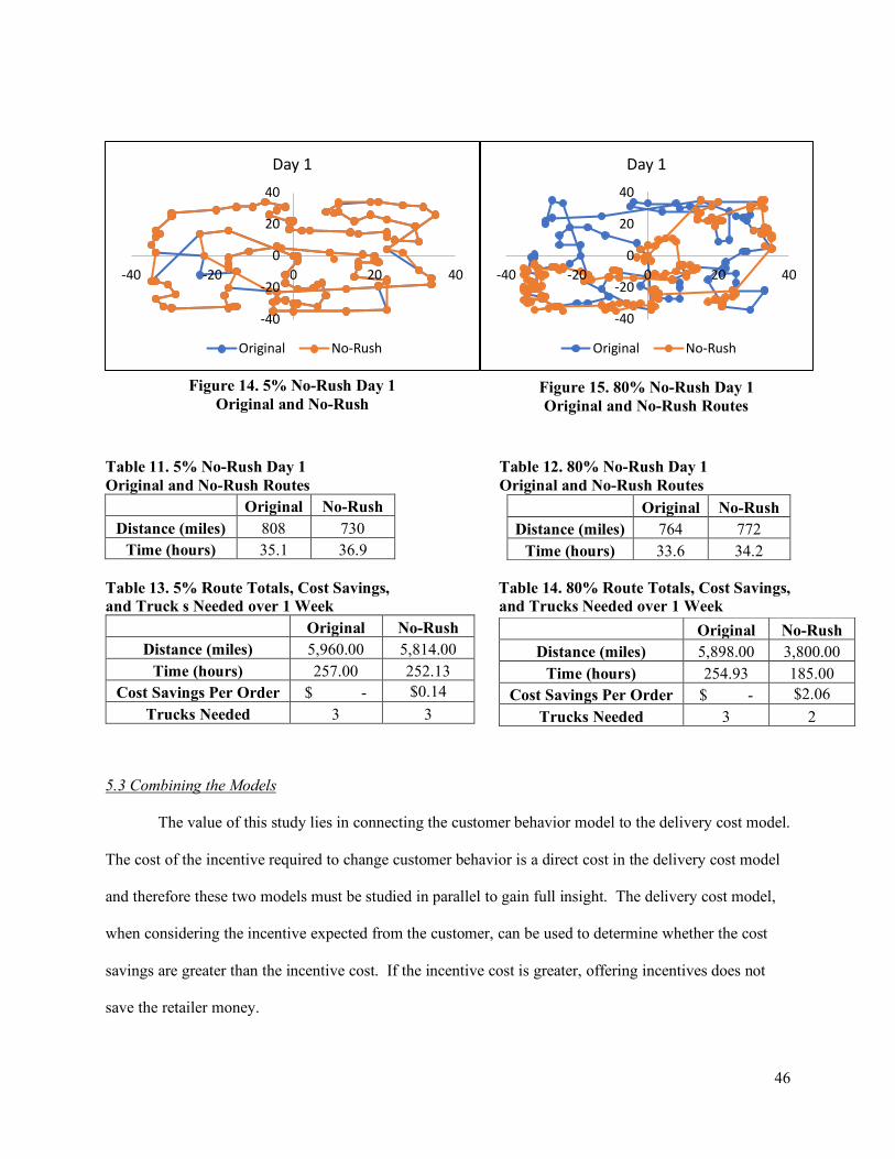
46
Table 11. 5% No-Rush Day 1 Table 12. 80% No-Rush Day 1 Original and No-Rush Routes Original and No-Rush Routes
Original No-Rush Distance (miles) 808 730
Time (hours) 35.1 36.9 Table 13. 5% Route Totals, Cost Savings, Table 14. 80% Route Totals, Cost Savings, and Truck s Needed over 1 Week and Trucks Needed over 1 Week
Original No-Rush Distance (miles) 5,960.00 5,814.00
Time (hours) 257.00 252.13 Cost Savings Per Order $ - $0.14
Trucks Needed 3 3
5.3 Combining the Models
The value of this study lies in connecting the customer behavior model to the delivery cost model.
The cost of the incentive required to change customer behavior is a direct cost in the delivery cost model
and therefore these two models must be studied in parallel to gain full insight. The delivery cost model,
when considering the incentive expected from the customer, can be used to determine whether the cost
savings are greater than the incentive cost. If the incentive cost is greater, offering incentives does not
save the retailer money.
Original No-Rush Distance (miles) 764 772
Time (hours) 33.6 34.2
Original No-Rush Distance (miles) 5,898.00 3,800.00
Time (hours) 254.93 185.00 Cost Savings Per Order $ - $2.06
Trucks Needed 3 2
-40
-20
0
20
40
-40 -20 0 20 40
Day 1
Original No-Rush
-40
-20
0
20
40
-40 -20 0 20 40
Day 1
Original No-Rush
Figure 14. 5% No-Rush Day 1 Original and No-Rush
Figure 15. 80% No-Rush Day 1 Original and No-Rush Routes
47
Input variables and percentage of customer buy-in have a large impact on the cost saving. This
study does not determine whether an individual retailer should offer incentives for no-rush shipping; nor
does it calculate the incentive that should be offered. Rather, it shows that there is a potential for cost
savings through incentivizing customers to make behavioral choices that are cost effective for the retailer.
The customer behavior model and the delivery cost model provide a framework with which a retailer can
determine whether incentivizing no-rush delivery makes sense for them, given their specific input values
and the demonstrated behavior of their customer base.
5.4 Limitations
The major limitations of this study were the use of a survey to collect customer data, the
assumptions made in the delivery cost model, and the simulated package data. A survey is a useful tool to
collect customer preferences and intentions, but is not necessarily a good measure of behavior. Sheffi and
Blanco (2018) point out that over 50% of consumers respond that they are willing to pay more for
sustainable products when surveyed, but in reality, only 15% of customers will pay more and only by a
small amount. While Sheffi and Blanco cite a significant limitation, it is important to note that
sustainability is a topic about which respondents want to look knowledgeable and involved. Regarding a
respondent’s willingness to accept a monetary incentive for longer delivery lead times, we believe that the
risk of untruthful responses is mitigated due to the lack of social pressure involved with this topic.
The delivery cost model assumed a single truck was making deliveries from a single distribution
center to customers within a 50-mile radius. The distribution area was assumed to be a grid with
Manhattan distances used to calculate the distance between nodes. An average of 100 packages per day
was randomly assigned to be delivered in a given 7-day week. All package deliveries were known
beforehand. This basic framework is useful in showing the criticality of the connection between
consumer behavior and its impact on routing. In reality, a retailer may be managing multiple trucks, at
multiple distribution centers. While Manhattan distances may be a good estimate of real travel distance,
most cities (other than Manhattan) are not laid out in grids. Many deliveries are made to rural areas. In

48
addition, retailers deal with a constant influx of orders rather than a predetermined list of weekly
deliveries and must be responsive in a dynamic environment.

49
6. CONCLUSION
While existing research studies consumer behavior and the influence of incentives, this study
shows that there is an impact of customer behavior on vehicle routing and cost. It is critical to combine
research of consumer behavior with a logistics cost model to determine the effectiveness of incentives to
drive cost savings. As behavior can be influenced by incentives provided by the retailer, the retailer can
influence behavior and thereby create cost savings. This study shows that by offering the correct
incentives, a logistic cost savings of 3-32% is possible depending on the percentage of customers who opt
in to no-rush delivery. Future studies can build on this foundation to determine incentives that can be
offered by specific retailers to their customers in a program to reduce logistics costs.
6.1 The Consumer Behavior Model
For each additional dollar of incentive, customers are willing to wait an additional 0.85 days for a
basic item ($1.18/day) and 0.88 days for a trendy item ($1.14/day). The most relevant variables when
determining a customer’s preferred lead time for a basic model are incentives, employment status,
whether the customer has dependents, and income. The most relevant variables when determining a
customer’s preferred lead time for a trendy item are incentives, the amount of time a customer usually
waits for delivery of an online purchase, and gender.
6.2 The Delivery Cost Model
Based on the proposed delivery network and assumed inputs, there is the potential for an average
of 3% to 32 % weekly logistic cost savings depending on the percent of customers who choose no-rush
delivery. If only 5% of customers opt in to no-rush delivery, it is possible for the cost of the incentives to
be greater than the logistic cost savings achieved. Above 5% no-rush, no trials were observed in which
the cost of delivery with a no-rush option was more expensive than the cost of delivery without the no-
rush option. Both the cost of the incentive and the likelihood of customers to choose the no-rush shipping
option should be considered by retailers when deciding to offer an incentivized no-rush delivery option.
50
6.3 Insights and Management Recommendations
Cost saving opportunities are critical to companies. Many of these initiatives require a cost that
saves money in the long run. This study shows that investing in incentives to influence customer
behavior can have delivery cost savings in the long-term. It is critical to study the specific products and
customers, and to study specific delivery networks and cost structures before offering incentives. With a
well understood customer base and a well-defined delivery network and routing procedure, providing a
no-rush delivery option to customers can lead to cost savings for retailers. In addition, a portion of the
cost savings comes from shorter route distances and therefore lower fuel consumption, which can also
have a positive environmental impact.
6.4 Future Research
This study opens avenues for additional research and provides the opportunity for more specific
models to further explore the impact of offering incentives on cost savings. Future research should
include a field study in partnership with a retailer. Customer behavior should be studied with incentives
actually offered at point-of-sale rather than with a survey. This field study will provide more accurate
data on consumer behavior than a survey will. Further study of customer behavior can refine the
correlation between customers and demographic characteristics, leading to an opportunity for retailers to
provide a no-rush shipping option to only the customers most likely to accept.
The impact of no-rush shipping and the cost of incentives on vehicle routing can be calculated in
the context of the retailer’s actual distribution network, including multiple trucks and distribution centers,
area maps per routing, and delivery fleet specific fuel cost, fuel efficiency, and labor costs. If necessary
for a specific retailer, an optimal (rather than heuristic solution) can be found. Actual (rather than
simulated) package delivery data should be used in future studies. Actual package and sales data will
allow the incorporation of observed trends in seasonality in the model. This framework can be expanded
into other industries, especially others that have different tiers of products which lead to different sets of
customer behavior.

51
REFERENCES Agatz, N., Campbell, A. M., Fleischmann, M., van Nunen, J., & Savelsbergh, M. (2013). Revenue management
opportunities for Internet retailers. Journal of Revenue and Pricing Management, 12(2), 128–138. https://doi.org/10.1057/rpm.2012.51
Amadeo, K. (2019). Four Critical Components of America’s Economic Growth. Retrieved May 3, 2019, from The Balance website: https://www.thebalance.com/components-of-gdp-explanation-formula-and-chart-3306015
Amadeo, K. (2018). The Retail Industry and Its Impact on the Economy. Retrieved May 3, 2019, from The Balance website: https://www.thebalance.com/what-is-retailing-why-it-s-important-to-the-economy-3305718
American Eagle Outfitters Men’s & Women’s Clothing, Shoes & Accessories. (n.d.). Retrieved November 23, 2018, from American Eagle Outfitters website: https://www.ae.com/content/help/shipping-handling
Asdemir, K., Jacob, V. S., & Krishnan, R. (2009). Dynamic Pricing of multiple home delivery options. European Journal of Operational Research, 196, 246–257.
Bell, D. R., Gallino, S., & Moreno, A. (2014). How to Win in an Omnichannel World. MIT Sloan Management Review, 56(1), 44–53. https://doi.org/10.1287
Berbeglia, G., Cordeau, J.-F., & Laporte, G. (2019). Dynamic pickup and delivery problems. European Journal of Operational Research, 202, 8–15.
Campbell, A. M., & Savelsbergh, M. W. P. (2005). Decision Support for Consumer Direct Grocery Initiatives. Transportation Science, 39(3), 313–327. https://doi.org/10.1287
Campbell, A. M., & Savelsbergh, M. (2006). Incentive Schemes for Attended Home Delivery Services. Transportation Science, 40(3), 327–341. https://doi.org/10.1287
https://doi.org/10.1287/inte.1090.0472 Chintagunta, P. K., Chu, J., & Cebollada, J. (2009). Quantifying Transaction Costs in Online/Offline Grocery
Channel Choice. Marketing Science, 31(1). https://doi.org/10.2307/41408452 Clarke, G., & Wright, J. W. (1962). Scheduling of Vehicles from a Central Depot to a Number of Delivery
Points. Fees and Timing | lululemon athletica. (n.d.). Retrieved November 23, 2018, from
https://info.lululemon.com/help/shipping/fees-and-timing Fisher, M. L., & Jaikumar, R. (1981). A Generalized Assignment Heuristic for Vehicle Routing. Networks, 11,
109–124. Fu, A. J., & Saito, M. (2018). “Would You Be Willing to Wait?”: Consumer Preference for Green Last Mile
Home Delivery. 64. Galante, N., López, E. G., & Monroe, S. (2013). The future of online grocery in Europe. Perspective on Retail
and Consumer Goods, 10. J.Crew Help : Shipping & Handling | J.Crew. (n.d.). Retrieved November 23, 2018, from
https://www.jcrew.com/help/shipping_handling.jsp?sidecar=true Lewis, M., Singh, V., & Fay, S. (2006). An Empirical Study of the Impact of Nonlinear Shipping and Handling
Fees on Purchase Incidence and Expenditure Decisions. Marketing Science, 25(1), 51–64. https://doi.org/10.1287/mksc.1050.0150
Macy’s Customer Service Site. (n.d.). Retrieved November 23, 2018, from https://www.customerservice-macys.com/app/answers/detail/a_id/86
Nordstrom Shipping, Pick Up in Store & More. (n.d.). Retrieved November 23, 2018, from Nordstrom website: https://shop.nordstrom.com/content/shipping-methods-charges
Parragh, S. N., Doerner, K. F., & Hartl, R. F. (2008). A survey on pickup and delivery problems: Part I: Transportation between customers and depot. Journal Für Betriebswirtschaft, 58(1), 21–51. https://doi.org/10.1007/s11301-008-0033-7
Rabinovich, E., Sousa, R., Park, S., & Golara, S. (2018). Omnichannel Retailing as a Balancing Act between In-Store and Home Fulfillment (SSRN Scholarly Paper No. ID 3113878). Retrieved from Social Science Research Network website: https://papers.ssrn.com/abstract=3113878
52
Sharma, S. K., Routroy, S., & Yadav, U. (2018). Vehicle routing problem: recent literature review of its variants. Int. J. Operational Research, 33(1), 1–31.
Sheffi, Y., & Blanco, E. (2018). Balancing green: when to embrace sustainability in a business (and when not to). Cambridge, MA: The MIT Press.
SSSD, A. M. R. (2019). US Census Bureau Monthly & Annual Retail Trade. Retrieved May 3, 2018, from https://www.census.gov/retail/index.html#ecommerce
Unni, S., Nair, V. S., & Gunasekar, S. (2015). E-retail and Online Customer Satisfaction: Differential Impact of Delivery Time in Indian Metros. Presented at the 2015 IEEE International Conference on Computational Intelligence and Computing Research 2015, December 10-12, Vickram College of Engineering, Enathi, Madurai, India. Retrieved from http://ieeexplore.ieee.org/servlet/opac?punumber=7430173
Vineyard Vines FAQ’s. (n.d.). Retrieved November 23, 2018, from https://www.vineyardvines.com/frequently-asked-questions/frequently-asked-questions.html#shipping
Yang, X., Strauss, A. K., Currie, C., & Eglese, R. (2013). Choice-Based Demand Management and Vehicle Routing in E-fulfilment (p. 29).
Zara Help-Shipping. (n.d.). Retrieved November 23, 2018, from https://www.zara.com/us/en/help/shipping-methods-and-pricing-h32.html
Zhang, Y., Luo, X., & Zeng, F. (2016). Omnichannel Promotion Effectiveness (p. 45). Retrieved from https://papers.ssrn.com/sol3/papers.cfm?abstract_id=2884190

53
APPENDIX A: Customer Behavior Survey

54
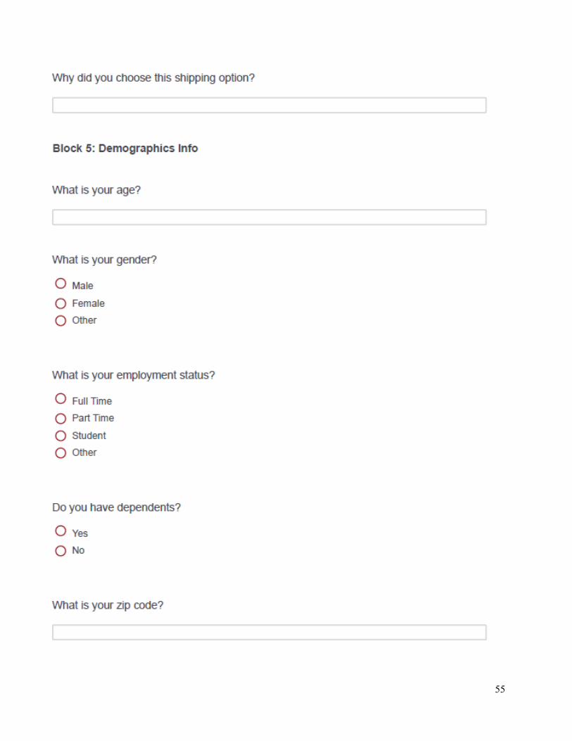
55

56

57
APPENDIX B: Vehicle Routing Heuristics Nearest Neighbor Heuristic
1. Select any node to be the active node (start with the origin)
2. Connect the active node to the closest unconnected node, making that the new active node
3. If there are more unconnected nodes, go to step 2, otherwise connect to the origin and end
Savings Algorithm
1. Start with a set of tours equal to the number of nodes, each beginning and ending at the origin and
visiting a single node
2. Calculate the savings associate with combining any 2 tours
3. Combine the tours that have the greatest savings
4. Repeat steps 2 and 3 until only a single tour is left
Cheapest Insertion Heuristic
1. For a subtour from the convex hull
a. Find the north-most, south-most, east-most, and west-most points and add them to the
convex hull
b. Find the center reference point by averaging all points on the convex hull
c. For each set of consecutive points
i. Draw a line between 2 consecutive points on the convex hull
ii. Find the point farthest from the line opposite the line from the refence point and
add it to the convex hull
d. Repeat b and c until no new points are added for a given iteration
2. Add to the tour the unconnected node that increases the cost (distance) the least, continue until all
nodes are connected

58
APPENDIX C: Survey Respondent Comments
Table C1. Survey Respondent Comment for Basic Item
Basic Item Offered $5 Incentive Offered $10 Incentive
Chose Standard Shipping
"time" "I want what I buy quickly." "For [necessity]" "easy to understand" "Since I [rely on] it." "Faster" "safe" "I like my shipping within a few days." "Always need an item sooner than later…" "2 day"
"Due to my interest" "More inexpensive" (note: the chosen option was not more inexpensive)
"Cash on delivery" "It makes you comfortable" "Cheaper" (note: chosen option was not cheaper) "[Fast] shipping is the best" "I prefer the quickest, simplest option" "it's faster" "speed is important" "it's good" "It’s better and quicker" "It's fast" "speed [of] delivery" "Because I want my purchased items to arrive quickly." "Fast and Convenient delivery" "to receive the item as quickly as possible"
I order many things online if I don't choose this option I might forget I had ordered something. We had chosen this option before and we had to leave town unexpectedly while waiting for an item somebody stole it and later it was a hassle trying to demonstrate what happened." "It is the most appropriate for my needs."
"Because it's fastest." "It's cheaper" (note: the chosen option was not cheaper) "I like to receive my order as quickly as possible." "COD" (cash on delivery)
"Am eagerly waiting for the item ordered" "to avoid additional charges" (note: the other option included a discount, not additional charges)
"That is convenient to me" "I want it as soon as possible and 40 dollars is not bad"
"instant gratification" "the best ecommerce website are all things to be excited for."
"I'm always antsy and prefer quick deliveries." "because I want the item quicker than 7 days."
Chose No-Rush Shipping
"I can usually wait, and the $10 off the order is a nice incentive to do so"
"Discount" "Discount offer" "To save $10"
"Because it's not an emergency and it's nice to have the discount for waiting. "
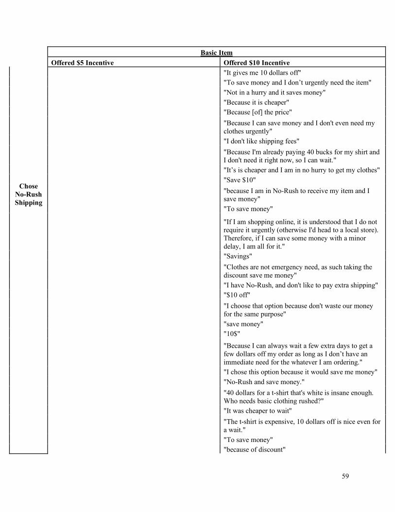
59
Basic Item Offered $5 Incentive Offered $10 Incentive
Chose
No-Rush Shipping
"It gives me 10 dollars off" "To save money and I don’t urgently need the item" "Not in a hurry and it saves money" "Because it is cheaper" "Because [of] the price"
"Because I can save money and I don't even need my clothes urgently"
"I don't like shipping fees"
"Because I'm already paying 40 bucks for my shirt and I don't need it right now, so I can wait."
"It’s is cheaper and I am in no hurry to get my clothes" "Save $10"
"because I am in No-Rush to receive my item and I save money"
"To save money"
"If I am shopping online, it is understood that I do not require it urgently (otherwise I'd head to a local store). Therefore, if I can save some money with a minor delay, I am all for it."
"Savings"
"Clothes are not emergency need, as such taking the discount save me money"
"I have No-Rush, and don't like to pay extra shipping" "$10 off"
"I choose that option because don't waste our money for the same purpose"
"save money" "10$"
"Because I can always wait a few extra days to get a few dollars off my order as long as I don’t have an immediate need for the whatever I am ordering."
"I chose this option because it would save me money" "No-Rush and save money."
"40 dollars for a t-shirt that's white is insane enough. Who needs basic clothing rushed?"
"It was cheaper to wait"
"The t-shirt is expensive, 10 dollars off is nice even for a wait."
"To save money" "because of discount"

60
Basic Item Offered $5 Incentive Offered $10 Incentive
Chose No-Rush Shipping
"time saved" (note: the chosen option does not save time)
"It's free, don't mind waiting"
"I rarely mind waiting. All my online shopping is done in advance. 10 dollars is a lot of money"
"because of the discount and my low level of necessity for the shirt"
"Cheaper in the long run" "Receiving $10.00 off my order"
"Because it is just a shirt and not that important to get quickly"
"I would rather save money than have the shirt a few days quicker. "
"The shirt is not an utmost necessity, I am capable of waiting in return for saving on the cost."
"I wanted to save $10 and don't need the items right away"
"for the discount" "To receive the discount" "because of offer"

61
Table C2. Survey Respondent Comments for Trendy Item Trendy Item
Offered $5 Incentive Offered $10 Incentive
Chose Standard Shipping
"time" "I want what I buy online quickly" "More trendy item vs. lower discount" "cost" (note: chosen option was more expensive)
"Fast delivery" "$10 off doesn't seem like much right now although I know it is...it's usually because I'll need the item faster"
"Since I [rely on] it." "Seems like a fun thing to have quickly to wear on a night out."
"quick receive" "2 day" "Faster delivery" "Better option"
"Most of my order I try to get them within 2 days." "Usually set standard shipping but depends on when I need if the discount would help"
"Because I am getting a good deal for something that is trending right now and the sooner I get it the better, before it goes out of style." "I'd rather have the [item from the] magazine quicker." "Due to my interest" "It’s fast"
"$5 wasn't worth the wait" "It’s cheap" (note: chosen option was not the cheapest option)
"Good shipping" "Since it is a new trend, the belated delivery may cause out of stock"
"faster" "The most appropriate to satisfy my needs." "If I order the latest trendy item of this week it's because I want to have it asap"
"it's better don't pay extra" (note: other option would have saved money)
"fast delivery" "Because this item is trendy and I would want to wear it right away"
"it's better" "because I want it now"
"It is new and trendy so I need it now. " "I would rather get item quicker than wait and get discount."
"To get the item quickly" "It's cheap" "Not to get late on the trend" "COD" (cash on delivery) "low price" "I need my item as fast as possible." "I want it fast if it is trendy I might want to wear it the same week. " "the discount isn't high enough to choose other option" "Because it's fastest." "Urgent required"
Chose No-Rush Shipping
"Even though the item is the latest trendy piece, I can still wait in order to get $10 off the order. The $10 is worth the wait."
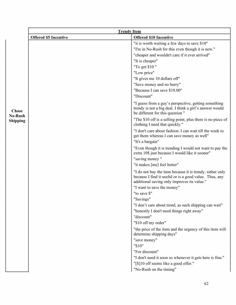
62
Trendy Item Offered $5 Incentive Offered $10 Incentive
Chose No-Rush Shipping
"it is worth waiting a few days to save $10" "I'm in No-Rush for this even though it is new." "cheaper and wouldn't care if it ever arrived" "It is cheaper" "To get $10 " "Low price" "It gives me 10 dollars off" "Save money and no hurry" "Because I can save $10.00" "Discount"
"I guess from a guy’s perspective, getting something trendy is not a big deal. I think a girl’s answer would be different for this question "
"The $10 off is a selling point, plus there is no piece of clothing I need that quickly."
"I don't care about fashion. I can wait till the week to get them whereas I can save money as well"
"It's a bargain"
"Even though it is trending I would not want to pay the extra 10$ just because I would like it sooner"
"saving money " "it makes [me] feel better"
"I do not buy the item because it is trendy, rather only because I find it useful or is a good value. Thus, any additional saving only improves its value."
"I want to save the money" "to save $" "Savings" "I don’t care about trend, as such shipping can wait" "honestly I don't need things right away" "discount" "$10 off my order"
"the price of the item and the urgency of this item will determine shipping days"
"save money" "$10" "For discount" "I don't need it soon so whenever it gets here is fine." "[$]10 off seems like a good offer." "No-Rush on the timing"
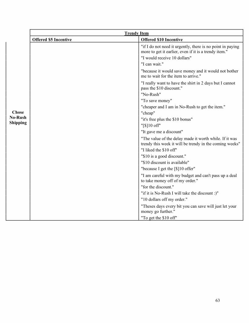
63
Trendy Item Offered $5 Incentive Offered $10 Incentive
Chose No-Rush Shipping
"if I do not need it urgently, there is no point in paying more to get it earlier, even if it is a trendy item."
"I would receive 10 dollars" "I can wait."
"because it would save money and it would not bother me to wait for the item to arrive."
"I really want to have the shirt in 2 days but I cannot pass the $10 discount."
"No-Rush" "To save money" "cheaper and I am in No-Rush to get the item." "cheap" "it's free plus the $10 bonus" "[$]10 off" "It gave me a discount"
"The value of the delay made it worth while. If it was trendy this week it will be trendy in the coming weeks"
"I liked the $10 off" "$10 is a good discount." "$10 discount is available" "because I get the [$]10 offer"
"I am careful with my budget and can't pass up a deal to take money off of my order."
"for the discount." "if it is No-Rush I will take the discount :)" "10 dollars off my order."
"Theses days every bit you can save will just let your money go further."
"To get the $10 off"

64
APPENDIX D: Median Route Visualization – Original vs. No-Rush 5% No-Rush
Figure D1. 5% No-Rush Day 1 Original Route and No-Rush Route
*Also shown in Section 5.2
Table D1. 5% No-Rush Day 1 Original Route and No-Rush Route Original No-Rush
Distance (miles) 764 772 Time (hours) 33.6 34.2
*Also shown in Section 5.2
Figure D2. 5% No-Rush Day 2 Original Route and No-Rush Route
Table D2. 5% No-Rush Day 2 Original Route and No-Rush Route
Original No-Rush Distance (miles) 888 912
Time (hours) 38.2 39.1
-40-30-20-10
010203040
-40 -30 -20 -10 0 10 20 30 40
Day 1
Original No-Rush
-40-30-20-10
010203040
-40 -30 -20 -10 0 10 20 30 40
Day 2
Original No-Rush

65
Figure D3. 5% No-Rush Day 3 Original Route and No-Rush Route
Table D3. 5% No-Rush Day 3 Original Route and No-Rush Route
Original No-Rush Distance (miles) 856 776
Time (hours) 35.9 33.0
Figure D4. 5% No-Rush Day 4 Original Route and No-Rush Route
Table D4. 5% No-Rush Day 4 Original Route and No-Rush Route
Original No-Rush Distance (miles) 890 854
Time (hours) 38.6 37.4
-40
-30
-20
-10
0
10
20
30
40
-40 -30 -20 -10 0 10 20 30 40
Day 3
Original No-Rush
-40
-30
-20
-10
0
10
20
30
40
-40 -30 -20 -10 0 10 20 30 40
Day 4
Original No-Rush

66
Figure D5. 5% No-Rush Day 5 Original Route and No-Rush Route
Table D5. 5% No-Rush Day 5 Original Route and No-Rush Route
Original No-Rush Distance (miles) 900 882
Time (hours) 38.9 38.3
Figure D6. 5% No-Rush Day 6 Original Route and No-Rush Route
Table D6. 5% No-Rush Day 6 Original Route and No-Rush Route
Original No-Rush Distance (miles) 832 804
Time (hours) 36.2 35.2
-40
-30
-20
-10
0
10
20
30
40
-40 -30 -20 -10 0 10 20 30 40
Day 5
Original No-Rush
-40
-30
-20
-10
0
10
20
30
40
-40 -30 -20 -10 0 10 20 30 40
Day 6
Original No-Rush

67
Figure D7. 5% No-Rush Day 7 Original Route and No-Rush Route
Table D7. 5% No-Rush Day 7 Original Route and No-Rush Route
Original No-Rush Distance (miles) 830 814
Time (hours) 35.5 34.6
Table D8. 5% Route Totals, Cost Savings, and Trucks Needed over 1 Week Original No-Rush
Distance (miles) 5,960.00 5,814.00 Time (hours) 257.00 252.13
Cost Savings Per Order $ - $0.14 Trucks Needed 3 3
*Also shown in Section 5.2
-40
-30
-20
-10
0
10
20
30
40
-40 -30 -20 -10 0 10 20 30 40
Day 7
Original No-Rush

68
20% No-Rush
Figure D8. 20% No-Rush Day 1 Original Route and No-Rush Route
Table D9. 20% No-Rush Day 1 Original Route and No-Rush Route
Original No-Rush Distance (miles) 818 830
Time (hours) 34.9 37.4
Figure D9. 20% No-Rush Day 2 Original Route and No-Rush Route
Table D10. 20% No-Rush Day 2 Original Route and No-Rush Route
Original No-Rush Distance (miles) 906 776
Time (hours) 38.8 35.8
-40
-30
-20
-10
0
10
20
30
40
-40 -30 -20 -10 0 10 20 30 40
Day 1
Original No-Rush
-40
-30
-20
-10
0
10
20
30
40
-40 -30 -20 -10 0 10 20 30 40
Day 2
Original No-Rush
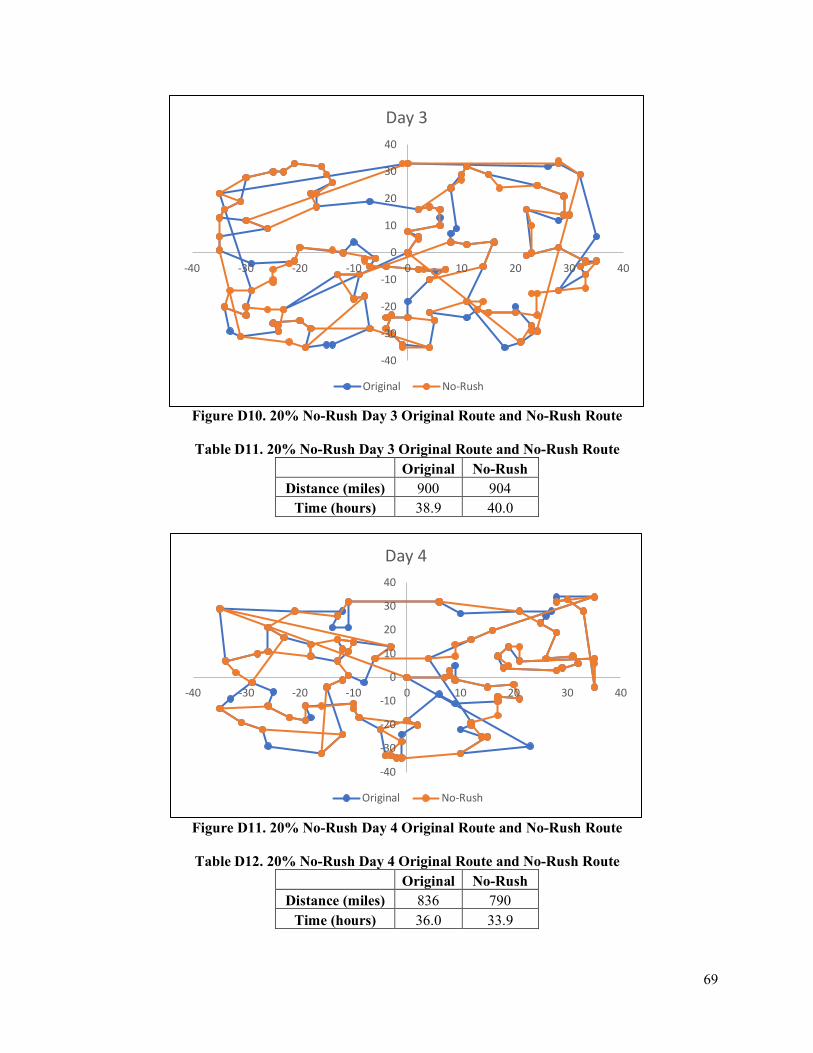
69
Figure D10. 20% No-Rush Day 3 Original Route and No-Rush Route
Table D11. 20% No-Rush Day 3 Original Route and No-Rush Route
Original No-Rush Distance (miles) 900 904
Time (hours) 38.9 40.0
Figure D11. 20% No-Rush Day 4 Original Route and No-Rush Route
Table D12. 20% No-Rush Day 4 Original Route and No-Rush Route
Original No-Rush Distance (miles) 836 790
Time (hours) 36.0 33.9
-40
-30
-20
-10
0
10
20
30
40
-40 -30 -20 -10 0 10 20 30 40
Day 3
Original No-Rush
-40
-30
-20
-10
0
10
20
30
40
-40 -30 -20 -10 0 10 20 30 40
Day 4
Original No-Rush
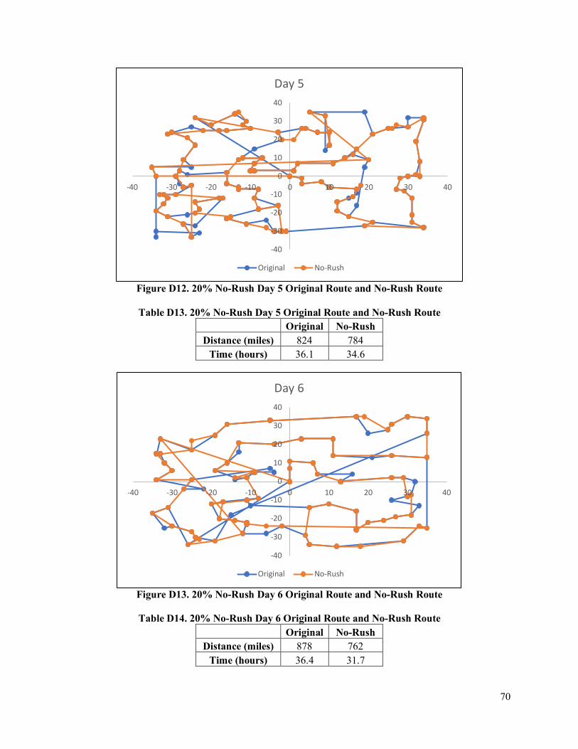
70
Figure D12. 20% No-Rush Day 5 Original Route and No-Rush Route
Table D13. 20% No-Rush Day 5 Original Route and No-Rush Route
Original No-Rush Distance (miles) 824 784
Time (hours) 36.1 34.6
Figure D13. 20% No-Rush Day 6 Original Route and No-Rush Route
Table D14. 20% No-Rush Day 6 Original Route and No-Rush Route
Original No-Rush Distance (miles) 878 762
Time (hours) 36.4 31.7
-40
-30
-20
-10
0
10
20
30
40
-40 -30 -20 -10 0 10 20 30 40
Day 5
Original No-Rush
-40
-30
-20
-10
0
10
20
30
40
-40 -30 -20 -10 0 10 20 30 40
Day 6
Original No-Rush

71
Figure D14. 20% No-Rush Day 7 Original Route and No-Rush Route
Table D15. 20% No-Rush Day 7 Original Route and No-Rush Route
Original No-Rush Distance (miles) 854 732
Time (hours) 36.6 30.6
Table D16. 20% Route Totals, Cost Savings, and Trucks Needed over 1 Week Original No-Rush
Distance (miles) 6,016.00 5,578.00 Time (hours) 258.87 244.27
Cost Savings Per Order $ - $0.43 Trucks Needed 3 3
-40
-30
-20
-10
0
10
20
30
40
-40 -30 -20 -10 0 10 20 30 40
Day 7
Original No-Rush
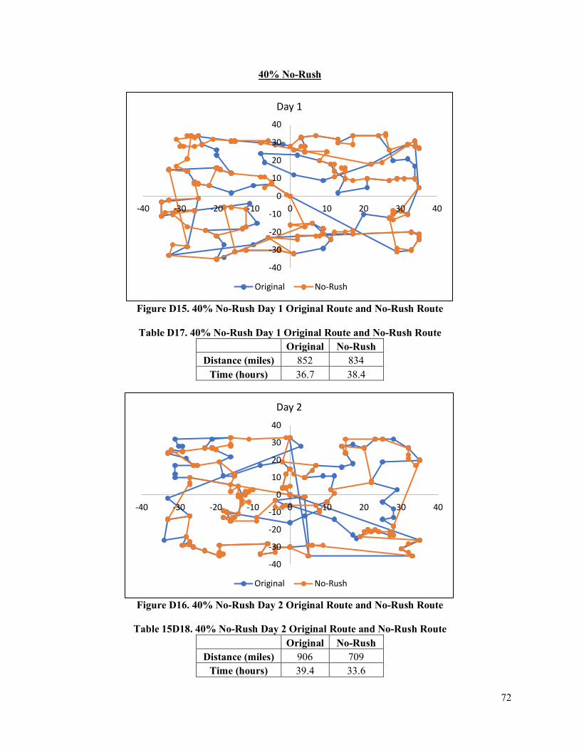
72
40% No-Rush
Figure D15. 40% No-Rush Day 1 Original Route and No-Rush Route
Table D17. 40% No-Rush Day 1 Original Route and No-Rush Route
Original No-Rush Distance (miles) 852 834
Time (hours) 36.7 38.4
Figure D16. 40% No-Rush Day 2 Original Route and No-Rush Route
Table 15D18. 40% No-Rush Day 2 Original Route and No-Rush Route
Original No-Rush Distance (miles) 906 709
Time (hours) 39.4 33.6
-40
-30
-20
-10
0
10
20
30
40
-40 -30 -20 -10 0 10 20 30 40
Day 1
Original No-Rush
-40
-30
-20
-10
0
10
20
30
40
-40 -30 -20 -10 0 10 20 30 40
Day 2
Original No-Rush

73
Figure D17. 40% No-Rush Day 3 Original Route and No-Rush Route
Table D19. 40% No-Rush Day 3 Original Route and No-Rush Route
Original No-Rush Distance (miles) 870 888
Time (hours) 36.7 39.9
Figure D18. 40% No-Rush Day 4 Original Route and No-Rush Route
Table D20. 40% No-Rush Day 4 Original Route and No-Rush Route
Original No-Rush Distance (miles) 874 764
Time (hours) 37.2 33.5
-40
-30
-20
-10
0
10
20
30
40
-40 -30 -20 -10 0 10 20 30 40
Day 3
Original No-Rush
-40
-30
-20
-10
0
10
20
30
40
-40 -30 -20 -10 0 10 20 30 40
Day 4
Original No-Rush
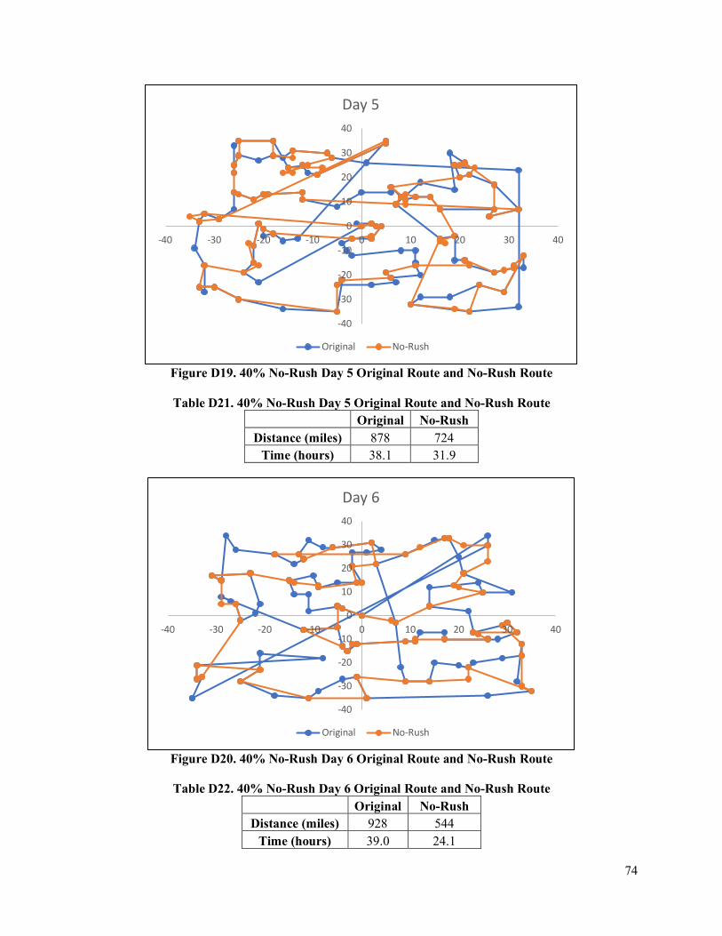
74
Figure D19. 40% No-Rush Day 5 Original Route and No-Rush Route
Table D21. 40% No-Rush Day 5 Original Route and No-Rush Route
Original No-Rush Distance (miles) 878 724
Time (hours) 38.1 31.9
Figure D20. 40% No-Rush Day 6 Original Route and No-Rush Route
Table D22. 40% No-Rush Day 6 Original Route and No-Rush Route
Original No-Rush Distance (miles) 928 544
Time (hours) 39.0 24.1
-40
-30
-20
-10
0
10
20
30
40
-40 -30 -20 -10 0 10 20 30 40
Day 5
Original No-Rush
-40
-30
-20
-10
0
10
20
30
40
-40 -30 -20 -10 0 10 20 30 40
Day 6
Original No-Rush
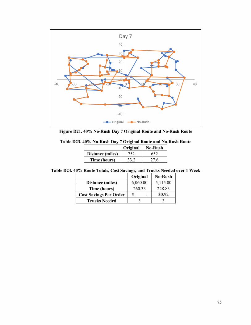
75
Figure D21. 40% No-Rush Day 7 Original Route and No-Rush Route
Table D23. 40% No-Rush Day 7 Original Route and No-Rush Route
Original No-Rush Distance (miles) 752 652
Time (hours) 33.2 27.6
Table D24. 40% Route Totals, Cost Savings, and Trucks Needed over 1 Week Original No-Rush
Distance (miles) 6,060.00 5,115.00 Time (hours) 260.33 228.83
Cost Savings Per Order $ - $0.92 Trucks Needed 3 3
-40
-30
-20
-10
0
10
20
30
40
-40 -30 -20 -10 0 10 20 30 40
Day 7
Original No-Rush
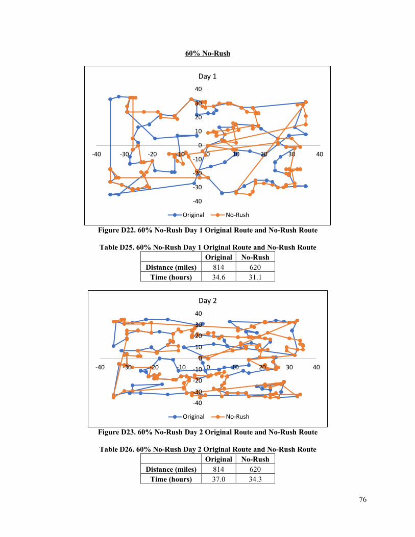
76
60% No-Rush
Figure D22. 60% No-Rush Day 1 Original Route and No-Rush Route
Table D25. 60% No-Rush Day 1 Original Route and No-Rush Route
Original No-Rush Distance (miles) 814 620
Time (hours) 34.6 31.1
Figure D23. 60% No-Rush Day 2 Original Route and No-Rush Route
Table D26. 60% No-Rush Day 2 Original Route and No-Rush Route
Original No-Rush Distance (miles) 814 620
Time (hours) 37.0 34.3
-40
-30
-20
-10
0
10
20
30
40
-40 -30 -20 -10 0 10 20 30 40
Day 1
Original No-Rush
-40-30-20-10
010203040
-40 -30 -20 -10 0 10 20 30 40
Day 2
Original No-Rush
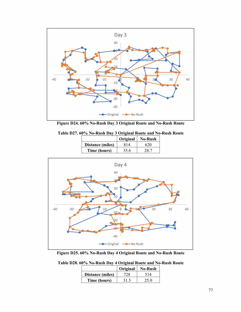
77
Figure D24. 60% No-Rush Day 3 Original Route and No-Rush Route
Table D27. 60% No-Rush Day 3 Original Route and No-Rush Route
Original No-Rush Distance (miles) 814 620
Time (hours) 35.6 28.7
Figure D25. 60% No-Rush Day 4 Original Route and No-Rush Route
Table D28. 60% No-Rush Day 4 Original Route and No-Rush Route
Original No-Rush Distance (miles) 728 514
Time (hours) 31.5 25.0
-40
-30
-20
-10
0
10
20
30
40
-40 -30 -20 -10 0 10 20 30 40
Day 3
Original No-Rush
-40
-30
-20
-10
0
10
20
30
40
-40 -30 -20 -10 0 10 20 30 40
Day 4
Original No-Rush
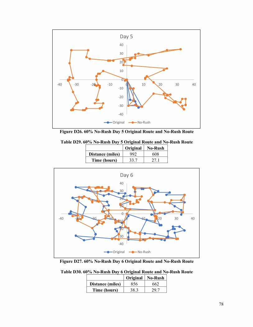
78
Figure D26. 60% No-Rush Day 5 Original Route and No-Rush Route
Table D29. 60% No-Rush Day 5 Original Route and No-Rush Route
Original No-Rush Distance (miles) 992 608
Time (hours) 33.7 27.1
Figure D27. 60% No-Rush Day 6 Original Route and No-Rush Route
Table D30. 60% No-Rush Day 6 Original Route and No-Rush Route
Original No-Rush Distance (miles) 856 662
Time (hours) 38.3 29.7
-40
-30
-20
-10
0
10
20
30
40
-40 -30 -20 -10 0 10 20 30 40
Day 5
Original No-Rush
-40
-30
-20
-10
0
10
20
30
40
-40 -30 -20 -10 0 10 20 30 40
Day 6
Original No-Rush
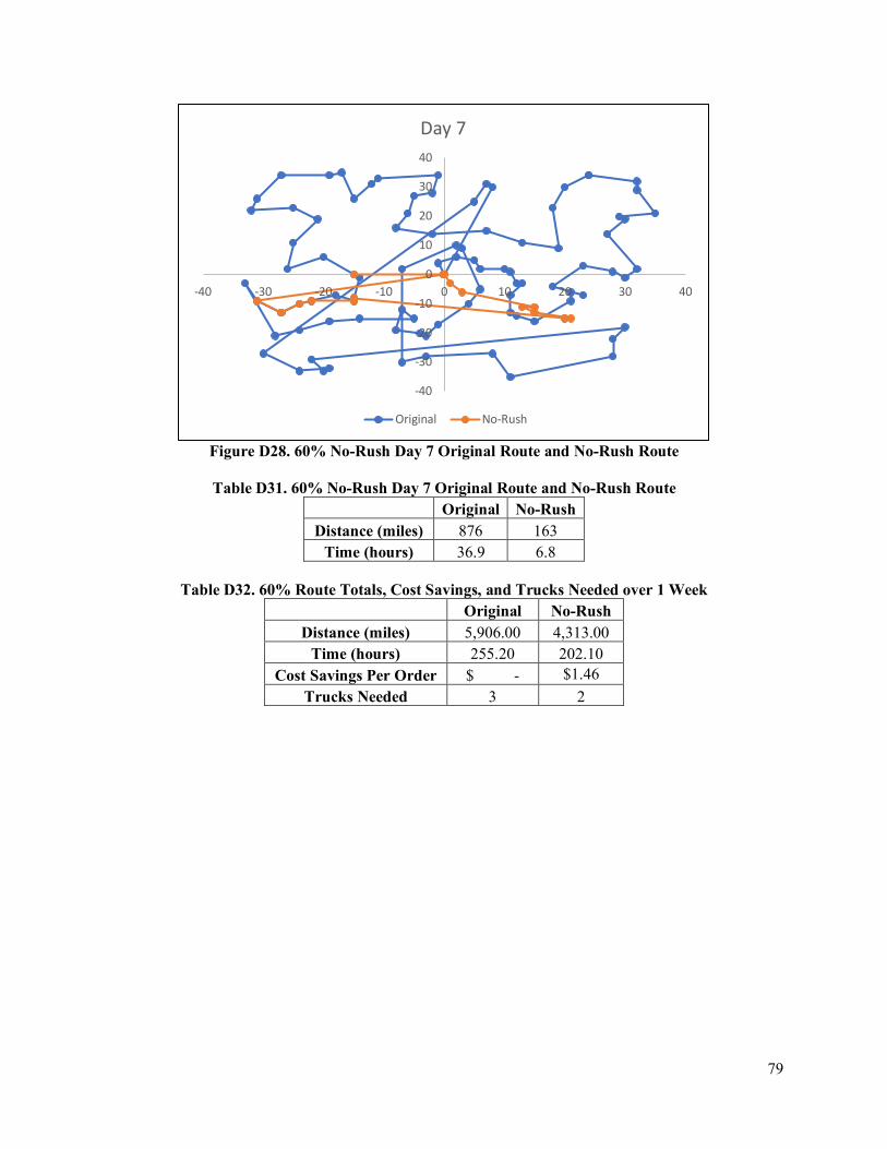
79
Figure D28. 60% No-Rush Day 7 Original Route and No-Rush Route
Table D31. 60% No-Rush Day 7 Original Route and No-Rush Route
Original No-Rush Distance (miles) 876 163
Time (hours) 36.9 6.8
Table D32. 60% Route Totals, Cost Savings, and Trucks Needed over 1 Week Original No-Rush
Distance (miles) 5,906.00 4,313.00 Time (hours) 255.20 202.10
Cost Savings Per Order $ - $1.46 Trucks Needed 3 2
-40
-30
-20
-10
0
10
20
30
40
-40 -30 -20 -10 0 10 20 30 40
Day 7
Original No-Rush

80
72% No-Rush
Figure D29. 72% No-Rush Day 1 Original Route and No-Rush Route
Table D33. 72% No-Rush Day 1 Original Route and No-Rush Route
Original No-Rush Distance (miles) 884 752
Time (hours) 38.1 38.1
Figure D30. 72% No-Rush Day 2 Original Route and No-Rush Route
Table D34. 72% No-Rush Day 2 Original Route and No-Rush Route
Original No-Rush Distance (miles) 900 936
Time (hours) 38.9 45.7
-40
-30
-20
-10
0
10
20
30
40
-40 -30 -20 -10 0 10 20 30 40
Day 1
Original No-Rush
-40-30-20-10
010203040
-40 -30 -20 -10 0 10 20 30 40
Day 2
Original No-Rush

81
Figure D31. 72% No-Rush Day 3 Original Route and No-Rush Route
Table D35. 72% No-Rush Day 3 Original Route and No-Rush Route
Original No-Rush Distance (miles) 764 512
Time (hours) 32.1 23.7
Figure D32. 72% No-Rush Day 4 Original Route and No-Rush Route
Table D36. 72% No-Rush Day 4 Original Route and No-Rush Route
Original No-Rush Distance (miles) 892 510
Time (hours) 38.7 24.4
-40
-30
-20
-10
0
10
20
30
40
-40 -30 -20 -10 0 10 20 30 40
Day 3
Original No-Rush
-40
-30
-20
-10
0
10
20
30
40
-40 -30 -20 -10 0 10 20 30 40
Day 4
Original No-Rush

82
Figure D33. 72% No-Rush Day 5 Original Route and No-Rush Route
Table D37. 72% No-Rush Day 5 Original Route and No-Rush Route
Original No-Rush Distance (miles) 876 610
Time (hours) 38.5 29.8
Figure D34. 72% No-Rush Day 6 Original Route and No-Rush Route
Table D38. 72% No-Rush Day 6 Original Route and No-Rush Route
Original No-Rush Distance (miles) 960 550
Time (hours) 40.3 23.3
-40
-30
-20
-10
0
10
20
30
40
-40 -30 -20 -10 0 10 20 30 40
Day 5
Original No-Rush
-40
-30
-20
-10
0
10
20
30
40
-40 -30 -20 -10 0 10 20 30 40
Day 6
Original No-Rush

83
Figure D35. 72% No-Rush Day 7 Original Route and No-Rush Route
*Also shown in Section 5.2
Table D39. 72% No-Rush Day 7 Original Route and No-Rush Route Original No-Rush
Distance (miles) 822 464 Time (hours) 34.2 17.6
*Also shown in Section 5.2
Table D40. 72% Route Totals, Cost Savings, and Trucks Needed over 1 Week Original No-Rush
Distance (miles) 6,098.00 4,344.00 Time (hours) 261.60 203.13
Cost Savings Per Order $ - $1.72 Trucks Needed 3 2
*Also shown in Section 5.2
-40
-30
-20
-10
0
10
20
30
40
-40 -30 -20 -10 0 10 20 30 40
Day 7
Original No-Rush
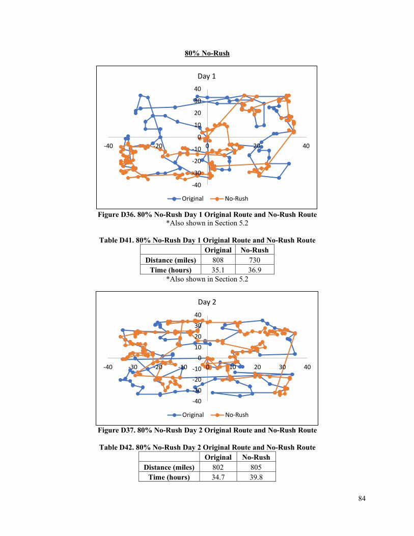
84
80% No-Rush
Figure D36. 80% No-Rush Day 1 Original Route and No-Rush Route
*Also shown in Section 5.2
Table D41. 80% No-Rush Day 1 Original Route and No-Rush Route Original No-Rush
Distance (miles) 808 730 Time (hours) 35.1 36.9
*Also shown in Section 5.2
Figure D37. 80% No-Rush Day 2 Original Route and No-Rush Route
Table D42. 80% No-Rush Day 2 Original Route and No-Rush Route
Original No-Rush Distance (miles) 802 805
Time (hours) 34.7 39.8
-40
-30
-20
-10
0
10
20
30
40
-40 -20 0 20 40
Day 1
Original No-Rush
-40-30-20-10
010203040
-40 -30 -20 -10 0 10 20 30 40
Day 2
Original No-Rush
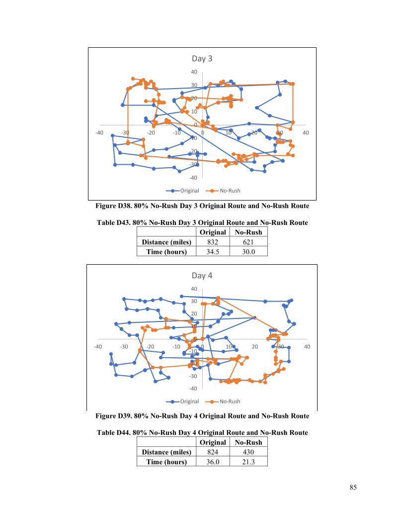
85
Figure D38. 80% No-Rush Day 3 Original Route and No-Rush Route
Table D43. 80% No-Rush Day 3 Original Route and No-Rush Route
Original No-Rush Distance (miles) 832 621
Time (hours) 34.5 30.0
Figure D39. 80% No-Rush Day 4 Original Route and No-Rush Route
Table D44. 80% No-Rush Day 4 Original Route and No-Rush Route
Original No-Rush Distance (miles) 824 430
Time (hours) 36.0 21.3
-40
-30
-20
-10
0
10
20
30
40
-40 -30 -20 -10 0 10 20 30 40
Day 3
Original No-Rush
-40
-30
-20
-10
0
10
20
30
40
-40 -30 -20 -10 0 10 20 30 40
Day 4
Original No-Rush

86
Figure D40. 80% No-Rush Day 5 Original Route and No-Rush Route
Table D45. 80% No-Rush Day 5 Original Route and No-Rush Route
Original No-Rush Distance (miles) 968 492
Time (hours) 41.7 24.0
Figure D41. 80% No-Rush Day 6 Original Route and No-Rush Route
Table D45. 80% No-Rush Day 6 Original Route and No-Rush Route
Original No-Rush Distance (miles) 822 326
Time (hours) 35.1 14.5
-40
-30
-20
-10
0
10
20
30
40
-40 -30 -20 -10 0 10 20 30 40
Day 5
Original No-Rush
-40
-30
-20
-10
0
10
20
30
40
-40 -30 -20 -10 0 10 20 30 40
Day 6
Original No-Rush

87
Figure D42. 80% No-Rush Day 7 Original Route and No-Rush Route
Table D47. 80% No-Rush Day 7 Original Route and No-Rush Route
Original No-Rush Distance (miles) 842 396
Time (hours) 37.5 18.5
Table D48. 80% Route Totals, Cost Savings, and Trucks Needed over 1 Week Original No-Rush
Distance (miles) 5,898.00 3,800.00 Time (hours) 254.93 185.00
Cost Savings Per Order $ - $2.06 Trucks Needed 3 2
*Also shown in Section 5.2
-40
-30
-20
-10
0
10
20
30
40
-40 -30 -20 -10 0 10 20 30 40
Day 7
Original No-Rush