43794400 circuitos electricos y maquinas en labview
TRANSCRIPT

Electrical Circuits and Machines Laboratory with LabVIEW™
June 2000 EditionPart Number 322765A-01
Electrical Circuits and Machines Laboratory with LabVIEW
Copyright
Copyright © 2000 by National Instruments Corporation,11500 North Mopac Expressway, Austin, Texas 78759-3504. Universities, colleges, and other educational nstitutions may reproduce all or part of this publication for educational use. For all other uses, this publication may not be reproduced or transmitted in any form, electronic or mechanical, including photocopying, recording, storing in an information retrieval system, or translating, in whole or in part, without the prior written consent of National Instruments Corporation.
TrademarksLabVIEW™ is a trademark of National Instruments Corporation.Product and company names mentioned herein are trademarks or trade names of their respective companies.
by Dr. Nesimi ErtugrulDepartment of Electrical and Electronic EngineeringUniversity of Adelaide

For More InformationFurther information about this laboratory can be obtained from the author: [email protected]
National Instruments Corporate Headquarters11500 North Mopac Expressway Austin, Texas 78759-3504 USA Tel: 512 794 0100
Worldwide OfficesAustralia 03 9879 5166, Austria 0662 45 79 90 0, Belgium 02 757 00 20, Brazil 011 284 5011, Canada (Calgary) 403 274 9391, Canada (Ontario) 905 785 0085, Canada (Québec) 514 694 8521, China 0755 3904939, Denmark 45 76 26 00, Finland 09 725 725 11, France 01 48 14 24 24, Greece 30 1 42 96 427, Germany 089 741 31 30, Hong Kong 2645 3186, India 91805275406, Israel 03 6120092, Italy 02 413091, Japan 03 5472 2970, Korea 02 596 7456, Mexico (D.F.) 5 280 7625, Mexico (Monterrey) 8 357 7695, Netherlands 0348 433466, New Zealand 09 914 0488, Norway 32 27 73 00, Poland 0 22 528 94 06, Portugal 351 1 726 9011, Singapore 2265886, Spain 91 640 0085, Sweden 08 587 895 00, Switzerland 056 200 51 51, Taiwan 02 2528 7227, United Kingdom 01635 523545
© National Instruments Corporation iii Electrical Circuits and Machines Laboratory with LabVIEW
Contents
Introduction
Lab 1Fundamentals of Magnetic Circuits
Magnetic Circuit Concept and Circuit Calculations................................................... 1-1Determination of the Hysteresis Characteristics of the Magnetic Circuits
and their Analysis..................................................................................................... 1-7
Lab 2Definitions and Measurement Technques in AC Circuits
Single-Phase AC Circuits and Definitions ................................................................. 2-1Power Definitions and Power Factor Correction in the Single-Phase AC Circuits.... 2-10Star/Delta and Delta/Star Conversion in the Three-Phase AC Circuits ..................... 2-17Voltage and Currents in the Star/Delta Connected AC Loads ................................... 2-21Voltage and Current Phasors in Three-Phase Systems............................................... 2-25Powers in Three-Phase AC Circuits ........................................................................... 2-29
Lab 3Electrical Machines Tests
Determination of the Moment of Inertia in the Rotating Machines ........................... 3-1Induction (Asynchronous) Motor ...............................................................................3-6Synchronisation of a Synchronous Generator ............................................................ 3-12
Lab 4Dynamic Simulation of Electrical Motors
Induction (Asynchronous) Motor Simulation............................................................. 4-1Dynamic Simulation of Brushless Permanent Magnet AC Motor Drives.................. 4-6Direct Current (DC) Motor Drive Simulation ........................................................... 4-12Additional References ................................................................................................ 4-16

Contents
Electrical Circuits and Machines Laboratory with LabVIEW iv www.ni.com
Appendix ALayout of the Laboratory and the Details of the Instrumentation

© National Instruments Corporation I-1 Electrical Circuits and Machines Laboratory with LabVIEW
Introduction
Within the last decade, the disciplines of electrical, electronics and computer engineering have become so intertwined. Although it is difficult to differentiate what separates these disciplines in terms of the theory, the experimental works related to each discipline have distinctive features, therefore, require special attention.
In this laboratory, LabVIEW software has been chosen as an enabling technology for programming, data capturing and data analysis. The hardware of the physical systems are monitored using the custom written software in LabVIEW. This courseware introduces interactive LabVIEW-based experiments into the curriculum of an Electrical Machines and Circuits course.
The overall mission of this interactive laboratory is to engage in both dedicated and interdisciplinary research studies and training facilities while providing life long experimental practices in areas related to Electrical and Electronic Engineering. It is believed that the prime benefits of this lab will be the deep understanding of electrical circuits, electrical machines and electromechanical devices, experiencing real-time signals and controls, and observing the limitations of the theory. However, it should be emphasised here that the above mission couldn’t be achieved without preliminary study and active participation in the practical tests. The preliminary preparation should include the study relevant section of the textbooks and the lecture notes in the area.
This laboratory is suitable for teaching the basic electrical engineering courses. The principal target audience is the first and the second year electrical engineering students. Furthermore, the VIs provided in Lab 4 can be utilized to study some advance control concepts in the area of the Electrical Machines and Drives

Introduction
Electrical Circuits and Machines Laboratory with LabVIEW I-2 www.ni.com
The fundamental approach used in this courseware is to keep the simulations as flexible as possible enabling the user to develop the range of applications using the principles presented here. Furthermore, due to the open structure of the VIs, they can later be modified to include the real-time VI modules as stated in the following sub-section.
The experiments in this handout are divided into four major groups. In each group a number of tests are presented. The tests in the main sections contain some background information to explain and conduct the experiments. In addition, some wiring diagrams are provided at the end of some sub-sections to guide towards the real-time implementations.
Lab 1 contains two tests about the magnetic circuits and the determination of BH characteristics. In Lab 2, many fundamental definitions and measurement techniques used in single-phase and three-phase AC circuits are studied. This section provides a very flexible and powerful display tools about “phasors”. Three Rotating Electrical Machine tests are given in Lab 3. The experiments presented in the section can easily be integrated into the real-time system. Lab 4 provides three advanced motor drive application VIs covering the Brushless Permanent Magnet Motors as well as two conventional motor drive simulation tools for the DC and the asynchronous motors.
In Real-Time ApplicationsAs mentioned earlier, at the end of some sections, the sample wiring diagrams are provided for the real-time implementation of the tests presented in the courseware. Since the hardware and the signal conditioning requirements for the laboratories in the educational institutions may vary, there is no fixed solution to implement the real-time systems. Please remember that the real-time tests require some modifications in the block diagrams of the VIs. To achieve this, please remove the simulated inputs and replace with a DAQ Sub-VI, which may contain a basic block diagram as shown in Figure 1. Secondly, make sure that suitable signal conditioning circuits are connected to the DAQ card and the measured signals are scaled correctly.

Introduction
© National Instruments Corporation I-3 Electrical Circuits and Machines Laboratory with LabVIEW
Figure 1. A sample sub-VI structure for the modification of the tests to implement real-time modules
In addition to this, please note that, the ratings of the real laboratory machines are not critical in the tests presented here. As stated earlier, the measured signals should be attenuated and isolated to a level that is safe for the DAQ systems and for the operators (students). The frequency bandwidth of the signal-conditioning device is also important for the accuracy of the measurement.
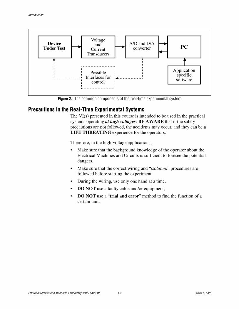
The essential parts of the real-time experimental system may consist of five principal units: a device under test, transducer(s), a PC and a data acquisition card, and custom-written software, which are all illustrated as a block diagram in Figure 2. Some of the minimum specifications of the experimental hardware that may be used in the real-time tests are listed below as a reference. The details of hardware used in the experiments are given later in the relevant sections under the heading “The specifications of the hardware used”.
Data acquisition system: at least 8 differential analog inports, 12-bit resolution, 100 kHz sampling frequency.
Computer: a Pentium PC, 32 MB RAM, and >1 GB hard disk,
Transducers: voltage and the current transducer unit(s), such as isolation amplifier(s) and Hall-Effect device(s), for signal conditioning and isolation purposes.
Devices Under Test: a rheostat, a single-phase transformer and the rotating electrical machines (a DC motor, an induction motor and a synchronous generator, and a DC tachogenerator all connected on a common shaft).
Introduction
Electrical Circuits and Machines Laboratory with LabVIEW I-4 www.ni.com
Figure 2. The common components of the real-time experimental system
Precautions in the Real-Time Experimental SystemsThe VI(s) presented in this course is intended to be used in the practical systems operating at high voltages: BE AWARE that if the safety precautions are not followed, the accidents may occur, and they can be a LIFE THREATING experience for the operators.
Therefore, in the high-voltage applications,
• Make sure that the background knowledge of the operator about the Electrical Machines and Circuits is sufficient to foresee the potential dangers.
• Make sure that the correct wiring and “isolation” procedures are followed before starting the experiment
• During the wiring, use only one hand at a time.
• DO NOT use a faulty cable and/or equipment,
• DO NOT use a “trial and error” method to find the function of a certain unit.
DeviceUnder Test
Voltageand
CurrentTransducers
A/D and D/Aconverter PC
Applicationspecificsoftware
PossibleInterfaces for
control

© National Instruments Corporation 1-1 Electrical Circuits and Machines Laboratory with LabVIEW
Lab 1Fundamentals of Magnetic Circuits
Magnetic Circuit Concept and Circuit Calculations
Educational ObjectivesAfter performing this experiment, students should be able to:
• Understand the basic concepts in the magnetic circuits,
• Analyse two typical magnetic circuits by using the simulation tools provided,
• Study the effects of changing the physical dimensions, the number of turns, and the fringing in magnetic circuits.
Reference Readings1. Circuits, Devices and Systems, R. Smith and R. Dorf, John Wiley and
Sons, 1992.
2. Electrical Machines, Drives and Power Systems, T. Wildi, Prentice Hall International, 1991.
3. Electrical Engineering: Principles and Applications, A.R. Hambley, Prentice Hall, 1997.
4. Electromechanical Energy Devices and Power Systems, Z.A. Yamayee and J.L. Bala, John Wiley and Sons, 1994.
Background InformationIn practice, many devices use some form of magnetic circuits that contain coils wound on magnetic materials, such as iron cores. In sizing the magnetic components during design stage, the approach of simple dc circuit analysis can be utilised. (Although there are some limitations in magnetic circuit approach, such as saturation, non-linearity, leakage and fringing flux).
To analyse the magnetic circuits, it is convenient to see the analogy between the electrical and the magnetic quantities. Hence the magnetic circuits can

Lab 1 Fundamentals of Magnetic Circuits
Electrical Circuits and Machines Laboratory with LabVIEW 1-2 www.ni.com
be simplified to take into account some of the difficulties in modelling some of the phenomena, such as fringing, which occur in the practical circuits. The principal assumptions in the analysis of magnetic circuits are listed below:
• If frequency <50 Hz, Ampere’s Law can be applied.
(1-1)
Here N is the number of turns, I is the current, Hk is the field intensity lmk is the mean length of the medium, magnetic core.
• Magnetic flux density B is uniform across the plane, therefore magnetic flux φ and magnetic field intensity H are constant, and H and φ have same direction.
(1-2)
Here B is the flux density, and A is the cross section of the uniform part of the magnetic section.
• Total flux entering a node is zero.
• A one dimensional circuit can be used instead of a three-dimensional magnetic field
• Each section of the path has a constant cross-sectional area
• The mean path length is used in all calculations
Figure 1-1. Sample magnetic circuits: 2-D representation, magnetic equivalent circuit illustrating the reluctance R, and the mmf source, NI.
In addition to these assumptions, if the fringing (the spreading of flux lines in an air-gap) exists, the flux density in the air-gap becomes less than the core, and it is impossible to calculate it analytically. However, the fringing can be taken into account by adding the length of the gap to each of the
N. I = ∑ mkk lH
φ = B.A
+
φφφφ
NI
RC
RGAP
NI
lmean(gap)
lmean(core)φ

Lab 1 Fundamentals of Magnetic Circuits
© National Instruments Corporation 1-3 Electrical Circuits and Machines Laboratory with LabVIEW
dimensions of the air-gap cross section (assuming that the cross sectional areas of each side of the air-gap are identical).
Once the magnetic equivalent circuit is obtained Ampere’s Law can be applied to determine the parameters of the circuit required. In the application of Ampere’s Law, depending upon the unknown parameter, one of the following methods can be used.
• Determination of Magnetomotive Force (mmf), NI, for a given flux density, B
• Determination of Magnetomotive Force for a given flux, φ• Determination of Flux for a given mmf (either by Trial and Error
Method or Graphical method)
In the simulation tools provided in this section, the first two analytical methods are used.
In a magnetic core, the magnetic flux density B is related to the magnetic field H according to the BH curve that is non-linear. The slope of this curve is known as the permeability of the material in henries per meter, µ. The relationship between B and H is given by
(1-3)
As will be seen from the BH relationship, the permeability depends on the operating value of magnetic flux density. In most of the cases, the electromagnetic devices are designed to operate within the linear section of the BH characteristic of the magnetic material. In the discussions presented here, it is assumed that the permeability of the magnetic material used in the core is constant, which is defined relative to the permeability of free space, µ0.
(1-4)
where µr is the relative permeability of the core.
The reluctance, magnetic resistance, of the magnetic circuit is given by R = l / µA, where l is the mean length and A is the cross sectional area of the uniform magnetic section.
Tasks to StudyTwo typical magnetic circuits are provided and analysed in this section. The simulations presented here are self-explanatory. The user may modify the input data (controlled by the control boxes provided) to view the corresponding calculated values on the indicators on the front panel.
B = µ H
µ = µr µ0

Lab 1 Fundamentals of Magnetic Circuits
Electrical Circuits and Machines Laboratory with LabVIEW 1-4 www.ni.com
In the test 1, Magnetics 1.vi is provided. Figure 1-2 illustrates the front panel and the explanations diagram of this VI. The second test about the magnetic circuit analysis has the front panel given in Figure 1-3, and it is named Magnetics 2.vi.
The problem definitions are given on the front panels of the associated VIs. In both VIs, the front panels have four distinct sub-sections. The top-left section displays the 3-D view of the magnetic circuit together with the control boxes of the physical dimensions of the magnetic core. 2-D magnetic equivalent circuit (that is analogous to the electrical circuit) is given on the top-right corner of the front panel. This section also animates the direction of the flux in the circuit and the polarity of the MMF source, and indicates the reluctance and the MMF source in the equivalent circuit. The other two sections on the front panels provide additional inputs and indicators that are based on the estimated values in the VIs.

Lab 1 Fundamentals of Magnetic Circuits
© National Instruments Corporation 1-5 Electrical Circuits and Machines Laboratory with LabVIEW
Figure 1-2. The front panel of Magnetics 1.vi, and the explanations panel
The simulated 3-D magnetic circuit is given here.Use the "numerical controls" to set the physicaldimensions of the circuit and the number of turnsof the coil.The parameters can be altered any time while theVI is running.
The equivalent magnetic circuit is illustrated heretogether with the directions of the flux in thecircuit.The numerical indicators provided in this sectiondisplay the parameters shown in the circuit.
The desired flux density in the air gap and therelative permeability of the core can be set here.To include "Fringing" effect and to change thepolarity of the supply tick the boxes. When"Reverse the Polarity" is ticked the figure and thecircuit are also modified.
In this section, all other indicators related to theanalysed circuit are displayed. When the settingschanged during the simulation, these values areupdated simultaneously.The estimated current value is displayed in"blue" colour.
“Problem definition”

Lab 1 Fundamentals of Magnetic Circuits
Electrical Circuits and Machines Laboratory with LabVIEW 1-6 www.ni.com
Figure 1-3. The front panel of Magnetics 2.vi, and the explanations panel
“Problem definition”
3-D magnetic circuit that will be simulated is given here.Use the "numerical controls" to set the physical dimensionsof the circuit and the number of turns of the coil. Theparameters can be altered any time.
The equivalent magnetic circuit isillustrated here together with thedirections of the fluxes. The numericalindicators display the calculatedparameters in the circuit
The other parameters of the core can be sethere. To include "Fringing" effect and tochange the polarity of the supply tick therelated boxes.
In this section, the indicators shows the estimatedvalues. When the settings changed during thesimulation, the values are updated simultaneously.The estimated flux and flux density values are alsodisplayed here.
Four of the calculated parameters aredisplayed here.

Lab 1 Fundamentals of Magnetic Circuits
© National Instruments Corporation 1-7 Electrical Circuits and Machines Laboratory with LabVIEW
Use the “continuous RUN button” to start the VI(s), and to study the following tasks:
• Using the default values, confirm that the indicated values are correct by the manual calculations.
• Change the relative permeability of the core and observe the variation on the reluctance of the core and the MMF. Did any other parameters vary? Why?
• Summarise the effects of changing the “Flux Density in the AirGap” (Test 1) and the “Current in the Coil” (Test 2).
• Alter the values of the number of turns and identify the most varying parameter(s).
• Vary the cross sectional area and the dimensions of the magnetic core and observe the variation of the reluctance value.
• The fringing describes the spreading of flux lines in an air gap of a magnetic circuit. While the simulation is running, Use the control, “Include Fringing” and observe the change in the value of “Cross sectional area of the air gap”.
• Observe the impact of the polarity change of the supply onto the direction of the flux and the polarity of MMF source.
Determination of the Hysteresis Characteristics of the Magnetic Circuits and their Analysis
Educational ObjectivesAfter performing this experiment, students should be able to:
• Understand the hysteresis phenomena in the magnetic circuits,
• Examine the hysteresis characteristics and estimate the hysteresis losses.
• Study the impact of the higher harmonics onto the voltage and current waveforms,
Reference Readings1. Circuits, Devices and Systems, R. Smith and R. Dorf, John Wiley and
Sons, 1992.
2. Electrical Machines, Drives and Power Systems, T. Wildi, Prentice Hall International, 1991.
3. Electrical Engineering: Principles and Applications, A.R. Hambley, Prentice Hall, 1997.
4. Electromechanical Energy Devices and Power Systems, Z.A. Yamayee and J.L. Bala, John Wiley and Sons, 1994.

Lab 1 Fundamentals of Magnetic Circuits
Electrical Circuits and Machines Laboratory with LabVIEW 1-8 www.ni.com
Background InformationIn an alternating current circuit surrounded by iron or other magnetic material, magnetic hysteresis occur, which is caused by the cyclic reversals of magnetic flux in the alternating magnetic field.
The alternating magnetic flux that is produced by the current induces a counter EMF in the electric circuit. Ideally, if the imposed EMF by the alternating current is a sine wave, the counter EMF and resulting the magnetic flux follows a sine wave. However, the alternating current waveform is greatly distorted in the magnetic circuits due to the phenomena called “magnetic saturation” in the cores of the magnetic circuit, and therefore it is not a sine wave.
The distorted wave of current can be resolved into two components: a true sine wave of equal effective intensity and power to the distorted wave, and higher harmonic components (also known as wattless component) that primarily consists of a triple harmonic.
As mentioned in the previous sections, in the magnetic circuits, there is a definite relationship between the flux density, B and the magnetic field intensity, H of a magnetic material, B = µ H. Here µ is the permeability of the medium. In free space, B and H are related by the constant, µo, known as the permeability of the free space, B = µo H.
In magnetic materials, the relationship between H and B is usually nonlinear and is expressed graphically by the BH curve of the material. For a cyclic input current waveform, a typical BH curve of a magnetic material (also known as hysteresis loop) is illustrated in Figure 1-4.
Figure 1-4. Typical BH curve of a magnetic circuit
In the hysteresis loop: when H = 0 the flux density is not zero but has a value ± Br, called the remnant magnetisation or residual flux density; similarly, when B = 0, the magnetic field is not zero, but is equal to ±Hc, a parameter
+ Hc
Br
- Br
- Hc Hm
Bm
- Bm

Lab 1 Fundamentals of Magnetic Circuits
© National Instruments Corporation 1-9 Electrical Circuits and Machines Laboratory with LabVIEW
called the coercive force of the material. As can be seen in the hysteresis loop curve, the slope of the curve’s incremental permeability (also know as the dynamic permeability) decreases with increasing B and ultimately reaches the permeability of the free space, µo. The state of low incremental permeability is known as “saturation”, and at this point, B = Bm and H = Hm.
A magnetic material absorbs energy during each cycle of the current and this energy is dissipated as heat. It is proven that the amount of heat (the loss) in the magnetic circuit is equal to the area of the hysteresis loop. Selecting a magnetic material that has a narrow hysteresis loop can reduce the hysteresis losses.
The BH curve shown in Figure 1-4 can easily be obtained if the magnetic circuit is operated on alternating current. In the circuit, H is proportional to this current flowing in the winding, and B is proportional to the integral of the voltage, v across the winding. This integral is the total flux linkage, λ = φ N.
(1-5)
λ = N B A (1-6)
Where N is the number of turns of the winding and A is the cross sectional area of the magnetic core.
Any distorted waveform can be traced to the harmonics it contains. Since the harmonic is any voltage and current waveform whose frequency is an integral multiple of the line frequency, a distorted waveform can be represented by a set of sine waves whose frequency, magnitude and phase angles are different than the fundamental waveform. The controls provided on the front panel of this test (Figure 1-5) could be utilized to construct a periodic voltage or current of any conceivable shape. To achieve this, use the fundamental component and add an arbitrary set of harmonic components (3rd and 5th harmonic components in this test).
The VI provided here has two different types of analysis states: reading from a data file (named RealTimeVoltageCurrent.txt) and reading the simulated input waveforms directly from the front panel settings. The real data file is named RealTimeVoltageCurrent.txt and contains a set of real measured data of the time, the voltage and the current waveforms of multiple periods. Use this data file to view the wave shapes of the real data in the practical magnetic circuit. However, a path name should be defined to read the text file automatically (see Figure 1-6).
λ(t) = ∫∫∫∫t
dtv0

Lab 1 Fundamentals of Magnetic Circuits
Electrical Circuits and Machines Laboratory with LabVIEW 1-10 www.ni.com
Figure 1-5. The front panel of BH Hysteresis.vi, and the explanations panel
The magnetic circuit under test. N1 is themain winding, and N2 is the search coilthat is used to measure the inducedvoltage, e in the circuit.
Use the controlsin this section toset theparameters in thesimulation. Thedesired voltageand currentwaveforms canbe obtained byusing the 3rd and5th harmoniccontrols.
The parameters ofthe magneticcircuit can be inputhere. The settingsare valid both inthe simulation andin the process ofthe real data that isavailable in thetext file provided.The path nameshould be definedto read the filenamed“RealTimeVoltageCurrent.txt.”
The voltage across the searchcoil is displayed in this graph(real or simulated).
The distorted supply current isdisplayed in this graph (Realor Simulated).
The flux estimated by usingthe induced voltage displayedin this graph is based on theequation:e = dλ/dt.
The BH characteristic of themagnetic circuit is shown here.
This section displays the estimatedvalues related to the BHcharacteristic, the estimated powerand the core losses of the circuit.
The title
Use these buttons to read the datafrom the text file or to select thesimulation mode, or to stop the test.

Lab 1 Fundamentals of Magnetic Circuits
© National Instruments Corporation 1-11 Electrical Circuits and Machines Laboratory with LabVIEW
Tasks to StudyAssume that the cross sectional area of the magnetic core is A, the mean length of its magnetic circuit is Lmean, and the core is wound with two coils of N1 and N2 turns. The winding N1 is excited by a distorted current varying cyclically from –Im to +Im. In this circuit, as the current varies, the flux will vary from –φm to +φm. The second winding N2 (search coil) is used to measure the induced voltage that is equal to e = -N2(dφ/dt). Perform the following tests.
• Select the button “Reading Real Data” and run the simulation (BH Hysteresis.vi.). Use the default values for the settings and read the text file named “RealTimeVoltageCurrent.txt”, which contains a set of real data in column format: sampling instants in second, the search coil voltage in volts and the winding current in amperes.
• Observe the variation of the current, the voltage, the flux linkage and the BH characteristic, and identify which waveforms are close to an ideal sine wave.
• Confirm manually that the indicated values of Br, Hc, Bm, and Hm are correct. You may use the hysteresis loop graph and change the scales to determine the numerical values accurately.
• Suggest some analytical solutions for the rms values of the voltage, the current and the flux linkage waveforms.
• While the VI is running, select the test mode “Using Simulated Waveforms” from the button, and alter the control parameters. Use the controls to set the current waveform that has a significant amount of triple harmonics, and observe the corresponding hysteresis loop until you obtain a B-H characteristic that is similar to the real B-H graph studied earlier.
• In the case of simulation, introduce some DC offset to the voltage and the current waveforms and report the changes on the graph of the flux linkage and the BH characteristic. Explain why there is a change in the graph.
• Vary the stacking factor and the cross sectional area of the core and observe the changes in the graphs and in the indicators. What conclusions can you draw from these changes?
Lab 1 Fundamentals of Magnetic Circuits
Electrical Circuits and Machines Laboratory with LabVIEW 1-12 www.ni.com
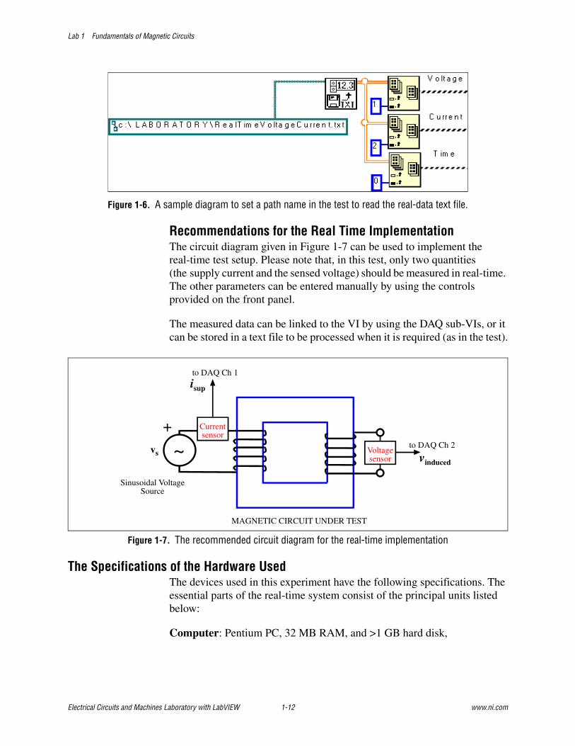
Figure 1-6. A sample diagram to set a path name in the test to read the real-data text file.
Recommendations for the Real Time ImplementationThe circuit diagram given in Figure 1-7 can be used to implement the real-time test setup. Please note that, in this test, only two quantities (the supply current and the sensed voltage) should be measured in real-time. The other parameters can be entered manually by using the controls provided on the front panel.
The measured data can be linked to the VI by using the DAQ sub-VIs, or it can be stored in a text file to be processed when it is required (as in the test).
Figure 1-7. The recommended circuit diagram for the real-time implementation
The Specifications of the Hardware UsedThe devices used in this experiment have the following specifications. The essential parts of the real-time system consist of the principal units listed below:
Computer: Pentium PC, 32 MB RAM, and >1 GB hard disk,
+vs vinduced
~Currentsensor
Voltagesensor
to DAQ Ch 1
to DAQ Ch 2
isup
MAGNETIC CIRCUIT UNDER TEST
Sinusoidal VoltageSource

Lab 1 Fundamentals of Magnetic Circuits
© National Instruments Corporation 1-13 Electrical Circuits and Machines Laboratory with LabVIEW
Data acquisition system: National Instruments AT-MIO-16E-10 data acquisition card with 8 differential A/D, 12-bit resolution, 100 kHz sampling frequency, 2 Analog Outputs (for 12-bit D/A conversion), 8 Digital I/O.
The device under test: The photo of the device under test and the specifications are given in Figure 1-8. Note that the device has a variable air gap allowing the user to carry out the tests at different conditions.
Figure 1-8. Photo of the device under test (a) and the equivalent magnetic circuit (b).
The main coil current: 300 mA max
Air gap gauges: 1mm, 2mm, 3mm, 4mm
Signal conditioning circuit: Please note that the real-time voltage of the search coil and the current of the main coil should be measured in this test. To achieve this, an in-house custom-built signal conditioning circuit has been used. The photo of the custom-built signal conditioning device and its block diagram are shown in Figure 1-9. This setup can provide a complete isolation and also allow the user to preform AC or DC tests on the device under test.
����������������������������������������������������������������������������������������������������
Searchcoil50turn
����������������������������������������������������������������������������������������������������������������������������������
Maincoil
1090turn
51mm
8mm
8mm57.7mm
8mm
a b

Lab 1 Fundamentals of Magnetic Circuits
Electrical Circuits and Machines Laboratory with LabVIEW 1-14 www.ni.com
Figure 1-9. Custom-built signal conditioning circuit and the block diagram.
Other auxiliary devices:Supply: 240V, 50 Hz
Auto transformer (for a variable voltage source): 240V, 8A, 50Hz
DCRectifierwith asmoothingcapacitor
AC input
Currentmeas.circuit
DUT(Main coil)
ACManual switchto selectthe excitation(AC or DC)
Controlsignal fromLabVIEW
a b

© National Instruments Corporation 2-1 Electrical Circuits and Machines Laboratory with LabVIEW
Lab 2Definitions and Measurement Technques in AC Circuits
Alternating current (AC) is used in a great variety of commercial and domestic applications. Furthermore, since electric power is generated and distributed as sinusoidal voltages and currents, the analysis of electric circuits with sinusoidal sources is very important. The analysis of AC circuits is regularly performed in the power systems. This involves the study of the performance of the system under both normal and abnormal conditions. However, such analysis requires a good understanding of the AC circuit theory. The tests provided in this section consider both single-phase and three-phase circuits. The basic definitions are also given and the fundamentals of the AC circuits are studied by using the virtual instrument approach.
Please note that in the tests presented here, it is assumed that steady-state sinusoidal condition is reached. This means that all transient effects after switching the signal on have disappeared, which eases the analysis of the AC circuits.
Single-Phase AC Circuits and Definitions
Educational ObjectivesAfter performing this experiment, students should be able to:
• Plot and interpret the characteristics of the sinusoidal current and the voltage waveforms,
• Understand the definitions of peak to peak value, peak and rms values, phase angle, complex impedance and base values (per-unit values) in the AC circuits.
• Study resistive, inductive and capacitive loads in single-phase AC circuits,
• Analyse the steady-state sinusoidal behaviour of the single-phase AC circuit using the phasors.

Lab 2 Definitions and Measurement Technques in AC Circuits
Electrical Circuits and Machines Laboratory with LabVIEW 2-2 www.ni.com
Reference Readings1. Electromechanical Energy Devices and Power Systems, Zia A. Yamaee,
L. Juan, and JR. Bala, John-Wiley and Sons, 1994.
2. Theory and Problems of Electric Circuits, J, A. Edminister, Schaum’s Outline Series, McGraw-Hill Book Company, 1972.
3. Electrical Machines, Drives, and Power Systems, T. Wildi, Prentice Hall, 1991.
4. N. Ertugrul, Electric Power Applications Lecture Notes, Department of Electrical and Electronic Engineering, University of Adelaide, 1997.
Background InformationA steady-state sinusoidal time-varying voltage signal (or current) can be given by
(2-1)
where v is the voltage, t is the time, Vm is the peak value (magnitude or amplitude), ω ω ω ω is the angular frequency, and θθθθ is the phase angle. The sinusoidal signals are periodic, repeating the same pattern of values in each period, T. The frequency of a periodic signal, f refers to the number of times the signal is repeated in a given time. The period is the time it takes for one cycle to be repeated, and the frequency, f and the period T are reciprocals of each other.
(2-2)
Peak to peak value is the difference between the highest and lowest values of the signal over one cycle. It would seem that it might be difficult to describe an AC signal in terms of a specific value, since an AC signal is not constant. However, to simplify the description, so called “effective value” is used. This value is the amount of DC signal which provides the same average value as the given AC signal. The effective value is also called the root-mean-square (RMS) value. The root-mean-square (RMS) value of the periodic waveform, for example the voltage v(t) is defined as
(2-3)
v(t) = Vm sin (ωt + θ)
f = 1/T
Vrms = ∫∫∫∫T
vT 0
2 dt(t)1

Lab 2 Definitions and Measurement Technques in AC Circuits
© National Instruments Corporation 2-3 Electrical Circuits and Machines Laboratory with LabVIEW
If a sinusoidal voltage is considered, the RMS value yields as
(2-4)
Please note that by convention, when a voltage or a current is described simply as AC, we refer to its RMS or effective value, not its maximum value.
ImpedanceThe impedance Z in AC circuits is defined as the ratio of voltage function to current function. The impedance is a complex number and can be expressed as
(2-5)
The real component of the impedance is called the resistance, R and the imaginary component is called the reactance, X. The reactance is a function of ωωωω in L and C loads. The impedance can also be displayed on the complex plane as the voltage and the current waveforms. However, since the resistance is never negative, only the first and the fourth quadrants are required.
PhasorsIn most of the AC circuit studies, the frequency is fixed, so this feature can be used to simplify the analysis. Sinusoidal steady-state analysis is greatly facilitated if the currents and voltages are represented as vectors in the complex number plane known as phasors. The basic purpose of phasor is to show the magnitude and phase angle between two or multiple quantities, such as voltage and current. The phasors can be defined in many forms (rectangular, polar, exponential, or trigonometric). However, the most common representation is the graphical form. As shown below for a voltage function, the rotating term at angular frequency ωωωω is ignored, and the phasor is illustrated by using the real part of a complex function in polar form.
(2-6)
Vrms = 2
Vm
Z = R ± jX
v(t) = Vm cos (ωt + θ)
= Re{ } ( )( ){ })()( 2Re tjjrms
tjm eeVeV ωθθω =+
Voltage phasor, V = Vrms eiθ = Vrms∠θ

Lab 2 Definitions and Measurement Technques in AC Circuits
Electrical Circuits and Machines Laboratory with LabVIEW 2-4 www.ni.com
This phasor is visualised as a vector of length Vrms that rotates counterclockwise in the complex plane with an angular velocity of ω. As the vector rotates, its projection on the real axis traces out the voltage as a function of time. The “phasor” is simply a snapshot of this rotating vector at t=0, as shown in the graph of the front panel.
In a linear circuit excited by sinusoidal sources, in the steady state, all voltages and currents will also be sinusoidal and of the same frequency. However, there may be a phase difference between the voltage and current depending upon the type of the load used. Three basic passive circuit elements, the resistor (R), the inductor (L) and the capacitor (C) are considered in this test. The AC load may be a combination of these passive elements: such as R+L and R+C.
Note that the current and voltage in the resistor are in phase, while L and C has 90° phase shift between voltage and current. The inductor current lags the inductor voltage by 90°; and. in the capacitor, the current leads the voltage by 90°.
Per-Unit ValuesThe per-unit system of measurement and computation is used in electrical engineering for two reasons:
• To eliminate the need for conversion of the voltages, currents and impedances in the circuit and to avoid using transformation from three-phase to single-phase and vice versa.
• To display multiple quantities on the same scale for comparison purpose.
The quantity that is subject to conversion is re-sized in terms of a particularly convenient unit, called the per-unit base of the system. Note that whenever per-unit values are given, they are always pure numbers. To calculate the actual values of the quantities, the magnitude of the base of the per-unit system must be known.
In electrical circuits, voltage, current, impedance and power can be selected as base quantities. If, however, voltage and power are selected, the quantities can be quite independent from each other as the base quantities. The reason behind this selection is that, the voltage/power per-unit system can automatically establish the corresponding base current and the base impedance.
However, the tests given here use the voltage and current as the base of the per-unit system, mainly due to the display purpose.

Lab 2 Definitions and Measurement Technques in AC Circuits
© National Instruments Corporation 2-5 Electrical Circuits and Machines Laboratory with LabVIEW
In the VI of this test, the voltage and the current waveforms simulate the measured values of voltage and current in the single-phase AC circuit. The equivalent impedance of the load is calculated and displayed on the front panel (as a per-unit value and a real value). Figure 2-1 illustrates the front panel and the explanations diagram of the VI under investigation.
In this VI, it is assumed that the current and voltage waveforms of a single-phase unknown load are measured (defined by the user), and the impedance of this unknown load is calculated. The complex impedance is displayed on the front panel and can be used to interpret the nature of the load (R, L , C, R+L or R+C). The phasor diagram is also provided to illustrate the concept of complex quantities in the graphical form, which is commonly used in the analysis of the AC systems.

Lab 2 Definitions and Measurement Technques in AC Circuits
Electrical Circuits and Machines Laboratory with LabVIEW 2-6 www.ni.com
Figure 2-1. The front panel and the explanations diagram of Single Phase AC Definitions.vi
Use these buttons to hide/show the currentwaveform and to set the base values for thecurrent and the voltage. Remember that thebase values are the peak (max) values.
This graph shows the phasor diagrams forthe voltage and the current. In the graph,the real and imaginary components of thevoltage phasor are also illustrated.Please refer to the legend of the graph toidentify the phasors.
These knobs can be used to set theamplitudes of the voltage and the current andthe phase angle.
This graph shows the voltage and the currentwaveforms of the single-phase AC circuit.
The base impedance and the real impedance(after the conversion) are displayed here in thecomplex form. The nature of the load is alsoindicated as "inductive", "capacitive" or "pureresistive".
The RMS values and the per-unit valuesof the voltage and current displayed in thegraph are shown here.

Lab 2 Definitions and Measurement Technques in AC Circuits
© National Instruments Corporation 2-7 Electrical Circuits and Machines Laboratory with LabVIEW
Tasks to Study• Run the VI named “Single Phase AC Definitions.vi” and vary the
values of the phase angle, the current amplitude and the voltage amplitude by using the knobs provided. Observe the relative positions of the voltage and current waveforms (phase angle) on the graph.
• Set the amplitudes of the voltage and the current equal to the base values, and analyse the estimated per-unit values of the voltage and current, and the rms values.
• Confirm that the impedance value displayed on the front panel is correct for the values entered.
• Without looking at the phasor diagram, plot the phasor diagram for the voltage and the current waveform that are shown on the waveform graph, and compare them with the displayed phasors. Is the load “resistive”, “capacitive” or “inductive”, and why?
• After the graphical observations of the voltage and current waveforms under three typical conditions (in phase, with lagging angle and leading phase angle), observe and record the impedances mathematically by the complex impedance equations. Record the complex impedance equations in the above studies and confirm the results by manual calculations. Notice that the impedances of both the pure inductor and the pure capacitor are pure imaginary numbers.
• In the case of R+L or R+C load, calculate the value of the inductance, L or the capacitor, C. Assume that the supply frequency is 60Hz.
Recommendations for the Real-Time ImplementationA sample wiring diagram given in Figure 2-2 can be used to implement the real-time test. As shown in the figure, only two parameters, the supply voltage and the line current, should be observed. In the real-time test, the knobs used in the simulation should be replaced with the DAQ controls since the amplitudes and the phase angle of the voltage and current are determined by the real-load and the real-supply voltage in the experimental setup.

Lab 2 Definitions and Measurement Technques in AC Circuits
Electrical Circuits and Machines Laboratory with LabVIEW 2-8 www.ni.com
Figure 2-2. A sample wiring diagram for the single-phase AC test
The Specifications of the Hardware UsedThe devices used in this experiment have the following specifications. The essential parts of the real-time system consists of the principal units listed below:
Computer: Pentium PC , 32 MB RAM, and >1 GB hard disk,
Data acquisition system: National Instruments AT-MIO-16E-10 data acquisition card with 8 differential A/Ds, 12-bit resolution, 100 kHz sampling frequency, 2 Analog Outputs (for 12-bit D/A conversion), 8 Digital I/O.
The device under test:Rheostat: 50 Ohm, 5 A
Signal conditioning devices:To achieve a complete electrical isolation, a hall-effect current transducer (50 A and 100 A, DC to 100 kHz) for the current measurement and an isolation amplifier (1000 V rms, 50 kHz) for the voltage measurement were employed. The block diagrams of the custom-built voltage and the current transducers, and the photo of the printed circuit board with the components loaded are shown in Figure 2-3.
+
~ RheostatLOAD : R,L
vs
to PCCh1
to PCCh 2
VOLTAGESENSOR
CURRENTSENSOR
Siusoidal supply

Lab 2 Definitions and Measurement Technques in AC Circuits
© National Instruments Corporation 2-9 Electrical Circuits and Machines Laboratory with LabVIEW
Figure 2-3. The basic circuit diagrams (a) and the photo of the custom-built current/voltage transducers (b)
Other auxiliary devices:Supply: 240V, 50 Hz
Auto transformer: 240V, 8A, 50Hz
~ 240V
VOLTAGEREGULATOR
(±15V)
Rm
AD711
M0
-+
BNCoutput
-
+
0-+
LA50-SDC/DCCONVERTER
+12V to
VOLTAGEREGULATOR
(±15V)
VOLTAGEREGULATOR
(+12V)
Voltage Attenuator
HighVoltage
Input
FUSE
~ 240V~ 240V
R2
R1
AD711IsolationAmpl.
ISO122P
BNCoutput
a
b

Lab 2 Definitions and Measurement Technques in AC Circuits
Electrical Circuits and Machines Laboratory with LabVIEW 2-10 www.ni.com
Power Definitions and Power Factor Correction in the Single-Phase AC Circuits
Educational ObjectivesAfter performing this experiment, students should be able to:
• Study complex power in the single-phase AC systems.
• Understand the power triangles,
• Study the requirements for the power factor correction and understand the concept.
Reference Readings1. Electromechanical Energy Devices and Power Systems, Zia A. Yamaee,
L. Juan, and JR. Bala, John-Wiley and Sons, 1994.
2. Theory and Problems of Electric Circuits, J, A. Edminister, Schaum’s Outline Series, McGraw-Hill Book Company, 1972.
3. Electrical Machines, Drives, and Power Systems, T. Wildi, Prentice Hall, 1991.
4. N. Ertugrul, Electric Power Applications Lecture Notes, Department of Electrical and Electronic Engineering, University of Adelaide, 1997.
Background InformationThe instantaneous power delivered to a load can be expressed as
(2-7)
The instantaneous power may be positive or negative depending upon the sign of v(t) and i(t), which is related to the sign of the signal at a given time. A positive power means that power flow from the supply to the load, and a negative value indicates that power flows from the load to the supply.
In the case of sine wave voltage and current, the instantaneous power may be expressed as the sum of two sinusoids, or as the sum of two sinusoids of twice the frequency as shown below.
(2-8)
p(t) = v(t) . i(t)
v(t) = Vm cos (ωt)
i(t) = Im cos (ωt + θ)
p(t) = Vm Im cos (θ) + Vm Im cos (2ωt+ θ)
p(t) = Vm Im cos θ . (1+ cos2ωt) + Vm Im sin θ . cos (2ωt+ π/2)
Lab 2 Definitions and Measurement Technques in AC Circuits
© National Instruments Corporation 2-11 Electrical Circuits and Machines Laboratory with LabVIEW
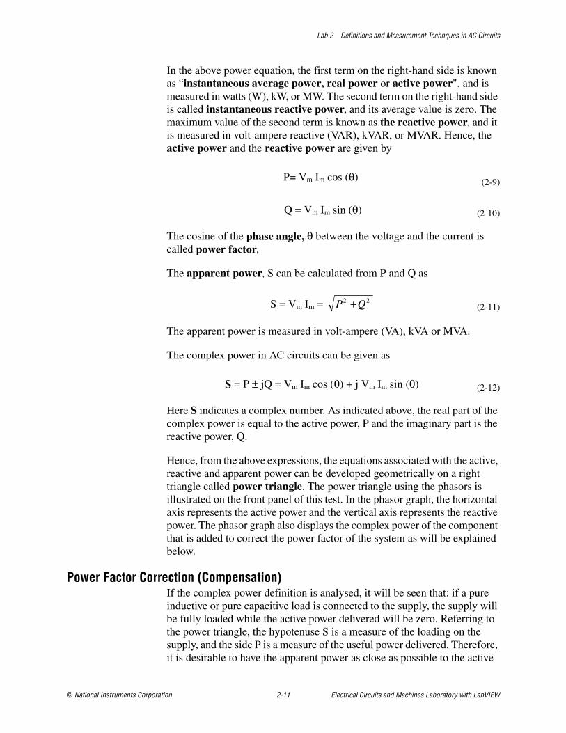
In the above power equation, the first term on the right-hand side is known as “instantaneous average power, real power or active power", and is measured in watts (W), kW, or MW. The second term on the right-hand side is called instantaneous reactive power, and its average value is zero. The maximum value of the second term is known as the reactive power, and it is measured in volt-ampere reactive (VAR), kVAR, or MVAR. Hence, the active power and the reactive power are given by
(2-9)
(2-10)
The cosine of the phase angle, θ between the voltage and the current is called power factor,
The apparent power, S can be calculated from P and Q as
(2-11)
The apparent power is measured in volt-ampere (VA), kVA or MVA.
The complex power in AC circuits can be given as
(2-12)
Here S indicates a complex number. As indicated above, the real part of the complex power is equal to the active power, P and the imaginary part is the reactive power, Q.
Hence, from the above expressions, the equations associated with the active, reactive and apparent power can be developed geometrically on a right triangle called power triangle. The power triangle using the phasors is illustrated on the front panel of this test. In the phasor graph, the horizontal axis represents the active power and the vertical axis represents the reactive power. The phasor graph also displays the complex power of the component that is added to correct the power factor of the system as will be explained below.
Power Factor Correction (Compensation)If the complex power definition is analysed, it will be seen that: if a pure inductive or pure capacitive load is connected to the supply, the supply will be fully loaded while the active power delivered will be zero. Referring to the power triangle, the hypotenuse S is a measure of the loading on the supply, and the side P is a measure of the useful power delivered. Therefore, it is desirable to have the apparent power as close as possible to the active
P= Vm Im cos (θ)
Q = Vm Im sin (θ)
S = Vm Im = 22 QP +
S = P ± jQ = Vm Im cos (θ) + j Vm Im sin (θ)

Lab 2 Definitions and Measurement Technques in AC Circuits
Electrical Circuits and Machines Laboratory with LabVIEW 2-12 www.ni.com
power, which makes the power factor approach 1. The process of making the power factor approach 1.0 (or below 1.0 but above the existing power factor) is known as power factor correction (or compensation).
In practice, the power factor correction is performed simply by placing a capacitor or an inductor across the existing load that itself may be an inductive or a capacitive load respectively. During the power factor correction process, the voltage across the load remains same and the active power does not change. However, the current and the apparent power drawn from the supply decrease. This means that the amount of decrease in supply current/power can be utilised somewhere else (by other loads) without increasing the capacity of the supply.
As an example: if the existing powers and the power factor of a single phase AC circuit are P= 1200 W, Q = 1600 var, S = 2000 VA, and pf = cos θ = 0.6 lagging, and we would like to correct the power factor to 0.9 lagging, a capacitor must be added across the load. After the correction is introduced, the active power remains unchanged but the apparent power is reduced to 1333 VA, and the reactive power of the capacitor equals to 1015 var leading.
The front panel of Single Phase Power and Power Factor Correction.vi is given in Figure 2-4. This VI provides a highly flexible virtual instrument to study the power and power factor correction in the single-phase AC circuits.

Lab 2 Definitions and Measurement Technques in AC Circuits
© National Instruments Corporation 2-13 Electrical Circuits and Machines Laboratory with LabVIEW
Figure 2-4. The front panel and the explanation diagram of the test Single Phase Power and Power Factor Correction.vi
Theseknobs canbe used tovary theamplitudeof thesupplyvoltage, theimpedanceof the loadand thefrequencyof thesupply.
This graph shows the phasordiagrams of the complex power(both for the inductive and thecapacitive load ing conditions),which is also known as "Powertriangle".
Use these buttons to hide orshow the relevantwaveforms on the abovegraph.
This graph shows the voltage and the currentwaveforms of the single-phase AC supply, andthe instantaneous power drawn from thesupply. The current of the component (L or C)that is added to correct the power factor of theload is also displayed.
Use the control to set thedesired power factor.Make sure that the desiredpower factor is greater thanthe power factor of the loadprior to the correction.
This picture ring displays the electriccircuit that represents the currentmode (with and without power factorcorrection).
Theindicatorsshow thecalculatednumericalvalues ofthe active,thereactiveand theapparentpowers inthe circuitthat isdisplayedin thepicturering.The statusof the loadpowerfactor isalso shownhere.

Lab 2 Definitions and Measurement Technques in AC Circuits
Electrical Circuits and Machines Laboratory with LabVIEW 2-14 www.ni.com
Tasks to StudyA number of tasks can be studied in this test. Although the combinations of settings can be many, it was found out that the following studies are sufficient to understand the concepts of the AC power and the power factor correction in the single-phase AC circuits. Furthermore, please note that these tests can easily be extended to analyse the multiple phase AC loads.
1. Set Voltage Amplitude = 339 V, Base Voltage = 339 V, Base Current = 10A, Rload=10 Ohm, Xload = 0 Ohm, f = 50 Hz and observe the waveforms of the voltage, the current, the power and the power phasors diagrams.
• What are the values of the active, the reactive, the apparent power and the power factor of the load? Confirm the displayed values by the manual computations.
• Have you noticed any change on the above power values when the “Desired Power Factor” is altered? Why?
2. Keep the rest of the settings but change only the value of the impedance to Rload = 0 Ohm, Xload = 10 Ohm, and observe the waveforms of the voltage, the current, the power and the power phasors.
• Now gradually increase the “Desired Power Factor” to the unity power factor 1.0, and observe the “Power Triangle” graph. What difference(s) have you noticed?
• What are the values of the active, the reactive, the apparent power and the power factor of the load before and after the power factor is corrected?
HINT: Observe the values for the two different cases: when the “Desired Power Factor” is less than pf(before) and when it is greater than the value of pf(before).
3. Set Voltage Amplitude = 339 V, Base Voltage = 339 V, Base Current = 10A, Rload = 0 Ohm, Xload = -10 Ohm, f = 50 Hz and observe the waveforms of the voltage, the current, the power and the power triangle.
• Gradually increase the “Desired Power Factor” to the unity power factor 1.0, and observe the “Power Triangle” graph. What difference have you noticed?
• What are the values of the active, the reactive, the apparent power and the power factor of the load before and after the power factor is corrected?
HINT: Same as the hint given above.

Lab 2 Definitions and Measurement Technques in AC Circuits
© National Instruments Corporation 2-15 Electrical Circuits and Machines Laboratory with LabVIEW
4. In this test, keep the rest of the settings but change only the value of the impedance to Rload = 10 Ohm, Xload = -10 Ohm, and observe the similar waveforms: the voltage, the current, the power and the power triangle.
• Gradually increase the “Desired Power Factor” to the unity power factor 1.0, and observe the “Power Triangle” graph again. Have you noticed any change, and why?
• What are the values of the active, the reactive, the apparent power and the power factor of the load before and after the power factor is corrected?
HINT: Same as the hint given above.
• Confirm the displayed values for the above case by the manual calculations.
5. Keep the rest of the parameters same as in the above section, but change the impedance to Rload = - 10 Ohm, Xload = 10 Ohm, and observe the waveforms: the voltage, the current, the power and the power triangle.
• Gradually increase “Desired Power Factor” to the unity power factor 1.0, and observe the “Power Triangle” graph. What difference have you noticed?
• What are the values of the active, the reactive, the apparent power and the power factor of the load before and after the power factor is corrected?
HINT: Same as the hint given above.
• Confirm the displayed values for the above case by the manual calculations.
• Compare the results obtained in 4 and 5.
Recommendations for the Real-Time ImplementationThe following circuit (Figure 2-5) can be employed to implement the real-time experiment for the test presented in this section. To do this, the supply voltage, the load current and the current of the external component (L or C) should be measured in real-time by the DAQ card.
However, the diagram of the VI should be modified considerably. To achieve this, firstly, remove the controls: Voltage Amplitude, Rload, Xload, Frequency, and Desired Power Factor. This is because such values will be determined by the external settings of the supply, the load and the additional components, C or L. Figure 2-5 provides a sample wiring diagram for an inductive load, in which the power factor is corrected by adding a capacitor. However, to achieve the desired power factor, the value of the capacitor should be determined in advance by the analytical computation. Please note that in Figure 2-5, the capacitor current can be estimated easily since icap = isup - iload.

Lab 2 Definitions and Measurement Technques in AC Circuits
Electrical Circuits and Machines Laboratory with LabVIEW 2-16 www.ni.com
Figure 2-5. The sample wiring diagram of the real-time power factor correction test. a) The circuit diagram without the Power Factor Correction, b) The circuit diagram to correct the power factor by adding a C.
The Specifications of the Hardware UsedThe devices used in this experiment have the following specifications.
Computer: Pentium PC , 32 MB RAM, and >1 GB hard disk,
Data acquisition system: National Instruments AT-MIO-16E-10 data acquisition card with 8 differential A/Ds, 12-bit resolution, 100 kHz sampling frequency, 2 Analog Outputs (for 12-bit D/A conversion), 8 Digital I/O.
The devices under test:Rheostat: 50 Ohm, 5 A,
Capacitor: 4µF, 1000V
Signal conditioning devices:In this experiment, the voltage and the current measurements are achieved by using the similar signal conditioning devices that were illustrated in Figure 2-3.
Other auxiliary instruments:Supply: 240V, 50 Hz
Auto transformer: 240V, 8A, 50Hz
+
~LOAD: R, L
vs
iloadisup
+
~vsC
iload
icap
isup
Currentsensor
isupply
Voltagesensor
to DAQ Ch 1
SinusoidalVoltageSource
LOAD: R, L
Currentsensor
vsupplyto DAQ Ch 2
iloadto DAQ Ch 3
a b
Lab 2 Definitions and Measurement Technques in AC Circuits
© National Instruments Corporation 2-17 Electrical Circuits and Machines Laboratory with LabVIEW
Star/Delta and Delta/Star Conversion in the Three-Phase AC Circuits
Educational ObjectivesAfter performing this test, students should be able to:
• Understand the star-delta or delta-star conversion required in the three-phase AC systems,
• Calculate and compare impedances of these two network configurations
Reference Readings1. Theory and Problems of Electric Circuits, Schaum’s Outline Series, J,
A. Edminister, McGraw-Hill Book Company, 1972.
2. N. Ertugrul, Electric Power Applications Lecture Notes, Department of Electrical and Electronic Engineering, University of Adelaide, 1997.
Background InformationAs known the electric power generation, transmission and distribution are accomplished with the three-phase systems. Although there are many single-phase loads in domestic and industrial use, these are assigned equally to the three-phases of the distribution system to achieve a balanced load, and most of the three-phase practical loads (such as three-phase AC motors) are balanced.
In a balanced three-phase system, since the sum of the phase currents is equal to zero, a neutral wire can be connected between the load neutral and the supply neutral. Hence, a single-phase consisting of one phase and a neutral wire can be analysed easily by using a single-phase equivalent circuit.
If a three-phase supply or a three-phase load is connected delta, it can be transformed into an equivalent star-connected supply or load. After the analysis, the results are converted back into their delta equivalent.
The delta/star or star/delta conversion formulas are given below, which are based on the electric circuit given in Figure 2-6.

Lab 2 Definitions and Measurement Technques in AC Circuits
Electrical Circuits and Machines Laboratory with LabVIEW 2-18 www.ni.com
(2-13)
(2-14)
Where Z is the complex impedance, Z = R ± jX.
Figure 2-6. The delta/star, star/delta electric equivalent circuits
When the load is balanced, the impedance per phase of the star connected load will be one-third of the impedance per phase of the delta-connected load. Hence the equivalent impedances can be given by
(2-15)
3
133221
Z
Z.ZZ.ZZ.ZZ
++++++++====A
2
133221
Z
Z.ZZ.ZZ.ZZ
++++++++====B
1
133221
Z
Z.ZZ.ZZ.ZZ
++++++++====C
CBA
BA
ZZZZ.Z
Z1 ++++++++====
CBA
CA
ZZZ
Z.ZZ2 ++++++++
====
CBA
CB
ZZZ
Z.ZZ3 ++++++++
====
ZA ZC
ZB
Z1 Z3
Z2
ZA = ZB = ZC = Z Z1 = Z2 = Z3 = 3Z

Lab 2 Definitions and Measurement Technques in AC Circuits
© National Instruments Corporation 2-19 Electrical Circuits and Machines Laboratory with LabVIEW
A three-phase AC supply is normally connected to a three-phase star or a delta connected balanced load. The front panel of this test (Star Delta Transformations.vi) is shown in Figure 2-7.
The VI is capable of transforming balanced and unbalanced three phase loads. One of the common uses of these transformation is in the three-phase transformer analysis. Circuit analysis involving three-phase transformers under balanced conditions can be performed on a per-phase basis. When ∆∆∆∆-Y or Y- ∆ ∆ ∆ ∆ connections are present, the parameters are referred to the Y side. In ∆∆∆∆- ∆ ∆ ∆ ∆ connections, the ∆∆∆∆ connected impedances are converted to equivalent Y connected impedances.
Tasks to Study• Set all impedances equal and perform ∆/Y and Y/∆ transformations,
• Repeat the above study by entering equal impedance values in each branch,
• Repeat the above study by setting unequal impedance values in each branch,
• Confirm the above results by the manual calculations.

Lab 2 Definitions and Measurement Technques in AC Circuits
Electrical Circuits and Machines Laboratory with LabVIEW 2-20 www.ni.com
Figure 2-7. The front panel and the explanation diagram of Star Delta Transformations.vi
This picture ringdisplays thecircuit connectionand theimpedanceequations.
This picture ringdisplays thecircuit connectionand theimpedanceequations, whichare convertedfrom the circuitdisplayed on theleft hand side.
This button changes the transformationbetween ∆/Y and Y/∆
These indicatorsdisplay theimpedances afterthe transformation.
Use the controls toinput theimpedances thatwill be transformedinto ∆ or Y.
The formulas used in thetransformation are shownhere.

Lab 2 Definitions and Measurement Technques in AC Circuits
© National Instruments Corporation 2-21 Electrical Circuits and Machines Laboratory with LabVIEW
Voltage and Currents in the Star/Delta Connected AC Loads
Educational ObjectivesAfter performing this test, students should be able to:
• Understand the definitions of phase and line voltages, and phase and line currents in the delta and star connected AC systems.
• Estimate and view the instantaneous voltage and currents in delta and star connected AC circuits.
Reference Readings1. Electromechanical Energy Devices and Power Systems, Zia A. Yamaee,
L. Juan, and JR. Bala, John-Wiley and Sons, 1994.
2. Theory and Problems of Electric Circuits, Schaum’s Outline Series, J, A. Edminister, McGraw-Hill Book Company, 1972.
3. Electrical Machines, Drives, and Power Systems, T. Wildi, Prentice Hall, 1991.
4. Electrical Engineering, Principles and Applications, A.R. Hambley, Prentice-Hall Inc., 1997.
Background InformationA three-phase AC system consists of three voltage sources that supply power to loads connected to the supply lines. The three-phase loads can be connected to the supplies either as “delta” or “star” configurations as stated previously.
In three-phase systems, the voltages differ in phase 1200, and their frequency and amplitudes are equal. If the three-phase loads are balanced (each having equal impedances), the analysis of such circuit can be simplified on a per-phase basis. This follows from the relationship that the per-phase real power, and reactive power are one-third of the total real power and reactive power respectively. It is very convenient to carry out the calculations in a per-phase star connected line to neutral basis. If ∆-Y , Y-∆ or ∆−∆ connections are present, the parameters on ∆ side(s) are transformed to Y connection, and computations are carried out.
Figure 2-8 shows two three-phase load connections that are commonly used in AC circuits. The loads are powered from a star connected three-phase supply.

Lab 2 Definitions and Measurement Technques in AC Circuits
Electrical Circuits and Machines Laboratory with LabVIEW 2-22 www.ni.com
Figure 2-8. Two common balanced-load connections in three-phase AC circuits
In an ideal three-phase supply, the frequencies and the magnitudes of each voltage source are equal, and therefore the supply voltages can be given as
(2-16)
v1s
v3s v2s
+
~3-phaseAC supply
~ +~+N
v23
v31v12
i1L
i2L
i3L
i31P
Z12=3Z
Z23 =3Z
v31p
v23p
Z31=3Z
i23P
v12p
i12P
v1s
v3s v2s
+
~
Z
Z
Z
3-phaseAC supply
~ +~+N n
v23
v31v
12
i1L
i2L
v3p
i3L
v1p
v2p
i1P
i2Pi3P
v1s(t) = Vm sin (ωt)
v2s(t) = Vm sin (ωt - 2π/3)
v3s(t) = Vm sin (ωt - 4π/3)

Lab 2 Definitions and Measurement Technques in AC Circuits
© National Instruments Corporation 2-23 Electrical Circuits and Machines Laboratory with LabVIEW
The similar expressions can be written for the current waveforms in the case of sinusoidal steady-state operation. Furthermore, four basic definitions are given for the voltages and the currents in the three-phase, usually as RMS values, not the maximum values.
• Phase voltage, such as v1s , v2s , v3s , v1p , v2p , v3p , v12p , v23p , v31p in Figure 2-8.
• Line-to-line voltage (or simply line voltage), such as v12 , v23 , v31 in Figure 2-8.
• Phase current, such as i1p , i2p , i3p , i12p , i23p , i31p in Figure 2-8.
• Line current, such as i1L , i2L , i3L in Figure 2-8.
A three-phase load is called "balanced" when the line voltages are equal and the line currents are equal. In a balanced three-phase system, there is a very simple relationship between the line and phase quantities, which can be obtained from the phasor quantities or the time varying expressions of the voltage and the current. The voltage and current relationships in three-phase AC circuits can be simplified by using the rms values (I and V) of the quantities. Referring to Figure 2-8, the following table can be given:
Figure 2-9 shows the front panel of the VI named “Voltage and currents in delta/star loads.vi”.
Star Connected Balanced Load Delta Connected Balanced Load
I1p =I1L , I2p =I2L , I3p =I3L
IL = I1L = I2L = I3L
Ip = IL /√√√√3
IL = I1L = I2L = I3L and Ip = I12p = I23p = I31p
Vp = VL /√√√√3
VL = V12 = V23 = V31
and Vp = V1p = V2p = V3p
V12 = V12p , V23 = V23p , V31 = V31p
VL = V12 = V23 = V31
The voltages across the impedances and the currents in the impedances are 120° out of phase
The voltages across the impedances and the currents in the impedances are 120° out of phase

Lab 2 Definitions and Measurement Technques in AC Circuits
Electrical Circuits and Machines Laboratory with LabVIEW 2-24 www.ni.com
Figure 2-9. The front panel of “Voltage and currents in delta/star loads.vi”, and the explanations panel.
Use the controls to setthe amplitude and thefrequency of thesupply. The buttonscan be used tohide/show the supplyside phase and linevoltages.
The load impedancecan be entered here.Use the buttons tohide/show the loadside phase currentsand voltages.
This picture ring illustrates the three-phaseAC circuit that is under investigation. Pleasenote that the load can be connected either asSTAR or DELTA, and the per-phaseimpedances are Z and 3Z respectively (whichcan be obtained from the star-deltatransformation).
This button controls the picturering shown above.
This graph displays the three-phasesinusoidal voltage and current waveformsat steady-state. To view and hide thewaveforms use the buttons provided on theleft-hand side of the panel, and make surethat you set base values for the voltage andthe current correctly.
The three-phasevoltage and currentwaveforms for circuitselected below aredisplayed here in thetime domain.
Please note that thevoltage and currentsare grouped andcoloured todistinguish the phaseand the line quantities.
Set the base valuesfor voltage andcurrent here to scalevoltage and currentsto be displayed onthe graph above.
The power factor of the loadis shown here.

Lab 2 Definitions and Measurement Technques in AC Circuits
© National Instruments Corporation 2-25 Electrical Circuits and Machines Laboratory with LabVIEW
Tasks to Study• Show that the line voltage Vline in the three-phase system is √3 times the
phase voltage, Vphase and confirm the result by running the VI for a given phase voltage.
• Study the above concept for the line currents and the phase currents in the case of delta connected load.
• In the above cases, find out the angles in “degrees” between the phase and line quantities on the supply and the load sides.
• Set the voltage and the load impedance(s) and calculate the phase currents. Use one-line equivalent circuit for this calculation since the load is balanced.
• Three incandescent lamps rated 60 W, 120V (rms) are connected in delta. What line voltage is needed so that the lamps burn normally. What are the line and phase currents in the circuit.
HINT: First calculate and set the resistance of the lamps using the controls provided.
• Three load resistors are connected in the delta form. If the line voltage is 415 V (rms) and the line current is 100 A (rms), calculate the current in each resistor, the voltage across the resistors and the resistance of each resistor. Confirm the results by the manual computations.
Voltage and Current Phasors in Three-Phase Systems
Educational ObjectivesAfter performing this test, students should be able to:
• Understand the phasors and the phase sequences in the three-phase balanced AC circuits.
Reference Readings1. Electromechanical Energy Devices and Power Systems, Zia A. Yamaee,
L. Juan, and JR. Bala, John-Wiley and Sons, 1994.
2. Theory and Problems of Electric Circuits, Schaum’s Outline Series, J, A. Edminister, McGraw-Hill Book Company, 1972.
3. Electrical Machines, Drives, and Power Systems, T. Wildi, Prentice Hall, 1991.
4. Electrical Engineering, Principles and Applications, A.R. Hambley, Prentice-Hall Inc., 1997.
5. N. Ertugrul, Electric Power Applications Lecture Notes, Department of Electrical and Electronic Engineering, University of Adelaide, 1997.

Lab 2 Definitions and Measurement Technques in AC Circuits
Electrical Circuits and Machines Laboratory with LabVIEW 2-26 www.ni.com
Background InformationAs can be seen in Equation 2-16, the voltage in Phase 1 reaches a maximum first, followed by Phase 2 and then Phase 3 for sequence 123. This sequence should be evident from the phasor diagram of the three-phase source where the phasors should pass a fixed point in the order 1-2-3, 1-2-3, ….
In this test, the variation of the phasors in a three-phase AC circuit will be examined. The phasors are obtained by selecting one of the voltage as the reference with a phase angle of zero, and determining the phase angles of the other two phases in the system. Since the amplitudes and the frequencies of the voltage sources are equal, the phasors have equal lengths and are drawn easily.
The phase and the line voltage phasors in the three-phase system can also be represented in polar form as shown below. However, please note that similar representation can be used for the current waveforms if the phase angle between the voltage and the current is known.
(2-17)
Where VPh is the phase voltage. Figure 2-10 shows the sequence and the shape of the voltage phasors in the three-phase star-connected AC circuit. There are two different ways to illustrate the phase and line voltages in the phasor form as shown in the figure. The dotted line in the figure demonstrates the line voltage phasors starting from origin, and this method is also used in this test.
oPhVV 901 −∠=
oPhVV 901 −∠=
oPhVV 901 −∠=
oPhVV 0323 ∠=
oPhVV 901 −∠=

Lab 2 Definitions and Measurement Technques in AC Circuits
© National Instruments Corporation 2-27 Electrical Circuits and Machines Laboratory with LabVIEW
Figure 2-10. The three-phase phasor representation.
2
1
3
1231
23
23
12
31
Line voltage
Phasevoltage
120o
30o
30o
30o

Lab 2 Definitions and Measurement Technques in AC Circuits
Electrical Circuits and Machines Laboratory with LabVIEW 2-28 www.ni.com
Figure 2-11. Front panel of 3phase phasors.vi and the explanations panel
These knobsand controls canbe used to setthe amplitude ofthe phasevoltages, thefrequency andthe phase angleof the three-phase ACsupply.
These equations represent the three-phase Phase and Line Voltages. Thevalues are updated depending uponthe input values. The format of theequations isv = Vm sin (ωt ± φ) = Vm sin (2πf t ±φ).
This figure illustrates the circuit diagram ofthe three-phase system under investigation.
Use thesebuttons tohide/show thevoltages and thephasors relatedto the phase andthe linevoltages.
This graph shows the three-phase Phaseand/or Line voltage waveforms in a starconnected system
This graph shows the three-phase Phase and/or Linevoltage phasors in a starconnected system
Lab 2 Definitions and Measurement Technques in AC Circuits
© National Instruments Corporation 2-29 Electrical Circuits and Machines Laboratory with LabVIEW
In this VI, two types of phasors are studied: one represents the phasors for the phase voltages and the second one illustrates the phasors for the line voltages. As it can be experimented, since one phase is always the reference, changing the phase angle effects all phasors equally and they rotate in the same direction as expected. The VI also displays the phase and the line voltages in the time domain.
Tasks to Study• Use the knobs provided on the front panel to vary the voltage amplitude,
the frequency and the phase angle (the angle between the voltage and current waveform), and observe the changes in the voltage and current phasors and the waveforms, and report your findings.
• Vary the phase angle Clockwise and Counterclockwise and observe the direction of the rotation of the phasors. Did the phase angles change, and why?
• Read the magnitude of each phasor and compare with the values set initially and with the values displayed in the time domain.
Note To simplify the comparisons, you may display either phase or line quantities simultaneously.
Powers in Three-Phase AC Circuits
Educational ObjectivesAfter performing this test, students should be able to:
• Understand the powers associated with the three-phase AC circuits.
• Investigate the power measurement techniques used in three-phase AC circuits.
Reference Readings1. Electromechanical Energy Devices and Power Systems, Zia A. Yamaee,
L. Juan, and JR. Bala, John-Wiley and Sons, 1994.
2. Theory and Problems of Electric Circuits, Schaum’s Outline Series, J, A. Edminister, McGraw-Hill Book Company, 1972.
3. Electrical Machines, Drives, and Power Systems, T. Wildi, Prentice Hall, 1991.
4. Electrical Engineering, Principles and Applications, A.R. Hambley, Prentice-Hall Inc., 1997.

Lab 2 Definitions and Measurement Technques in AC Circuits
Electrical Circuits and Machines Laboratory with LabVIEW 2-30 www.ni.com
Background InformationSince the phase impedances of a balanced star or delta connected load contain equal currents, the phase power is one-third of the total power. As a definition, the voltage across the load impedance and the current in the impedance can be used to compute the power per phase as explained in the Power Definitions and Power Factor Correction in the Single-Phase AC Circuits section.
Let us assume that the angle between the voltage and the current is θ, which is equal to the angle of the impedance. Considering the load configurations given in Figure 2-12, the phase power and the total power can be estimated easily.
In the case of Figure 2-12a, the phase active power and the total active power are
(2-18)
(2-19)
Figure 2-12. Delta-connected load (a) and star connected load.
Since the line current Iline = √3 Iphase in the balanced delta connected loads, if this equation is substituted into the equation ( 2-19), the total active load becomes
(2-20)
P1 = P2 = P3 = P = Vline Iphase cosθ
Ptotal = 3 x P = 3 Vline Iphase cosθ
iL
iL
iL
i31P
v31p
v23p
Z
i23P
v12p
i12P
P1
Z
Z
Z
Z
Z
n
iL
iL
v3p
iL
v1p
v2p
i1P
i2Pi3P
P1
Ptotal = √√√√3 Vline Iline cosθθθθ

Lab 2 Definitions and Measurement Technques in AC Circuits
© National Instruments Corporation 2-31 Electrical Circuits and Machines Laboratory with LabVIEW
In Figure 2-12b, however, the impedances contain the line currents, Iline (= phase current, Iphase) and the phase voltages, Vphase (=Vline/√3). Therefore, the phase active power and the total active powers are
(2-21)
(2-22)
If the relationship between the phase voltage and the line voltage (Vphase = Vline/√3) is used, the total active power becomes identical to the equation developed in Equation 2-20. This means that, the total power in any balanced three-phase load (∆ or Y connected) is given by Equation 2-20, √3 Vline Iline cos θθθθ, where θ is the angle on the load impedance.
Similarly, the total reactive and the total apparent power in the three-phase balanced AC circuits can be given by
(2-23)
(2-24)
Power MeasurementsIn the three-phase power systems, one, two or three wattmeters can be used to measure the total power. A wattmeter may be considered to be a voltmeter and an ammeter combined in the same box, which has a deflection proportional to VI cosθθθθ where θ is the angle between the voltage and current. The wattmeter has two voltage and 2 current terminals, which have + or – polarity signs. Three power measurement methods utilising the wattmeters are described below and are given in the VI (Three phase power measurements.vi), which are applied to the balanced three-phase AC load.
Two Wattmeter MethodThe method can be used in a three-phase three-wire balanced or unbalanced load system that may be connected ∆ or Y. To perform the measurement, two wattmeters are connected as shown in Figure 2-13.
P1 = P2 = P3 = P = Vphase Iline cosθ
Ptotal = 3 x P = 3 Vphase Iline cosθ
Qtotal = √3 Vline Iline sin θ
Stotal = √3 Vline Iline

Lab 2 Definitions and Measurement Technques in AC Circuits
Electrical Circuits and Machines Laboratory with LabVIEW 2-32 www.ni.com
In the balanced loads, the sum of the two wattmeter-readings gives the total power. This can be proven in a star-connected load mathematically as
(2-25)
Figure 2-13. Power Measurement by two wattmeters in star or delta-connected load
Figure 2-14. The three-phase voltage phasors used in the two wattmeter method
P1 = V12 I1 cos (300 + θ) = Vline Iline cos (300 + θ)
P2 = V32 I3 cos (300 - θ) = Vline Iline cos (300 - θ)
Ptotal = P1 + P2 = = √3 Vline Iline cos θ
v1s
v3s v2s
+
~3-phaseAC supply
~ +~+N
3-WIRE THREE-PHASEBALANCED LOAD
STAR OR DELTA CONNECTED
+V
+I
+V
+I
n
Z
Z Z
Wattmeter 1
Wattmeter 2
30o
θθθθ V1
I1
V2n
V3n
V3
I3 V12

Lab 2 Definitions and Measurement Technques in AC Circuits
© National Instruments Corporation 2-33 Electrical Circuits and Machines Laboratory with LabVIEW
If the difference of the readings is computed
(2-26)
which is 1/√3 times the total three-phase reactive power. This means that the two wattmeter method can also indicate the total reactive power in the three-phase loads.
Three Wattmeter MethodThis method is used in a three-phase four-wire balanced or unbalanced load. The connections are made with one meter in each line as shown in the figure below (Figure 2-15). The total active power supplied to the load is equal to the sum of the three wattmeter-readings.
(2-27)
Figure 2-15. The wattmeter connections in the three-phase four-wire loads
One Wattmeter MethodThe method is suitable only in three-phase four-wire balanced loads. The connection of the wattmeter is similar to the drawing given in Figure 2-15. The total power is equal to three times the reading of only one wattmeter that is connected between one of the phase and the neutral terminal.
In Figure 2-16, the front panel of the VI named “Three phase power measurements.vi” is given. Please refer to the explanations figure for the individual functions of the controls given on the front panel, which are similar to the earlier VIs.
P2 – P1 = Vline Iline cos (300 - θ) - Vline Iline cos (300 + θ) = Vline Iline sin θ
Ptotal = P1 + P2 + P3
v1s
v3s v2s
+
~
Z
3-phaseAC supply
~ +~+N
n
N
4-WIRE THREE-PHASESTAR-CONNECTEDBALANCED LOAD
+V
+V
+V
+I
+I
+I
Z
Z
Wattmeter 1
Wattmeter 3
Wattmeter 2
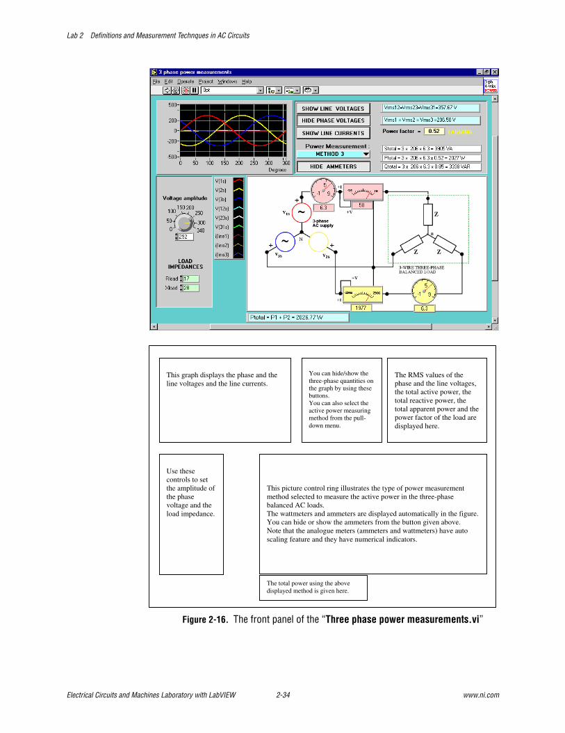
Lab 2 Definitions and Measurement Technques in AC Circuits
Electrical Circuits and Machines Laboratory with LabVIEW 2-34 www.ni.com
Figure 2-16. The front panel of the “Three phase power measurements.vi”
This graph displays the phase and theline voltages and the line currents.
Use thesecontrols to setthe amplitude ofthe phasevoltage and theload impedance.
You can hide/show thethree-phase quantities onthe graph by using thesebuttons.You can also select theactive power measuringmethod from the pull-down menu.
The RMS values of thephase and the line voltages,the total active power, thetotal reactive power, thetotal apparent power and thepower factor of the load aredisplayed here.
This picture control ring illustrates the type of power measurementmethod selected to measure the active power in the three-phasebalanced AC loads.The wattmeters and ammeters are displayed automatically in the figure.You can hide or show the ammeters from the button given above.Note that the analogue meters (ammeters and wattmeters) have autoscaling feature and they have numerical indicators.
The total power using the abovedisplayed method is given here.
Lab 2 Definitions and Measurement Technques in AC Circuits
© National Instruments Corporation 2-35 Electrical Circuits and Machines Laboratory with LabVIEW
Tasks to Study• Make sure that you studied and understood the power in the single-phase
AC circuits that was presented in the Power Definitions and Power Factor Correction in the Single-Phase AC Circuits section.
• A balanced three-phase, three-wire star-connected load is connected to a three-phase supply. The line voltage is 400V. The load comprises of an impedance of 100 + j100 Ohms per phase. Set these parameters and select the suitable circuit to determine the total active, reactive and apparent power by using the VI provided.
• Assume that the above load is a four-wire circuit. Use three power measurement methods and confirm your findings manually.
• Three 10µF capacitors are connected in STAR (wye) across a 2300 V (rms, line voltage), 60 Hz line. Calculate the line current, the active power, the reactive power and the apparent power by using the VI.
• A three-phase heater dissipates 15 kW when connected to a 208V, three-phase line. Determine the value of each resistor if they are connected as STAR.
• An industrial plant draws 600 kVA from a 2.4 kV line at a power factor of 0.8 lagging. What is the equivalent line-to-neutral impedance of the plant?
• An electric motor having a power factor 0.82 draws a current of 25A from a 600V three-phase AC supply. Find out the active power supplied to the motor.
Recommendations for the Real-Time ImplementationThis test can be modified to accommodate the power measurement in the three-phase AC circuits in real-time. However, additional sub-VI designs are needed to include the real-time DAQ facilities.
Depending upon the type of the circuit (balanced, unbalanced, 3-wire, 4-wire), the number of A/D channels may vary. The wiring circuit given below can provide the most flexible configuration, which can be used in any three-phase AC circuit regardless of the type of the load. Please note that, the load is star connected here. Please note that if the star-point is not accessible (either from the supply side or from the load side, an artificial star-point (fourth-wire) may be created by using the three identical high value resistors connected star across the terminals. If the load is delta-connected, however, the three-phase power can be measured only by the “two-wattmeter method”.

Lab 2 Definitions and Measurement Technques in AC Circuits
Electrical Circuits and Machines Laboratory with LabVIEW 2-36 www.ni.com
Figure 2-17. A sample wiring diagram for the real-time three-phase power measurement.
As shown above, only the phase voltages and the line currents are measured. The active, the reactive and the apparent power can be computed from these quantities after the phase angle is determined, which is the angle between say Phase 1 voltage and Line 1 current.
The specifications of the hardware usedThe devices used in this experiment have the following specifications.
Computer: Pentium PC , 32 MB RAM, and >1 GB hard disk,
Data acquisition system: National Instruments AT-MIO-16E-10 data acquisition card with 8 differential inputs, 12-bit resolution, 100 kHz sampling frequency, 2 Analog Outputs (for 12-bit D/A conversion), 8 Digital I/O.
The devices under test:Three rheostats to form a three-phase load (star-connection), each 50 Ohm, 5 A.
Signal conditioning devices:In this experiment, the voltage and the current measurements are obtained by using the identical signal conditioning devices that were given in Figure 2-3.
v1s
v3s v2s
+
~
Z3
3-phaseAC supply
~ +~+N
n
N
Z1
Z2
Currentsensor
Voltagesensor
to DAQ Ch 5v2
Currentsensor
Voltagesensor
Voltagesensor
Currentsensor
to DAQ Ch 2i2line
to DAQ Ch 3i3line
to DAQ Ch 1i1line
to DAQ Ch 6v3
to DAQ Ch 4v
1
THREE-PHASE LOAD

Lab 2 Definitions and Measurement Technques in AC Circuits
© National Instruments Corporation 2-37 Electrical Circuits and Machines Laboratory with LabVIEW
Other auxiliary instruments:Supply: 3-phase, 415V, 50 Hz
A 3-phase auto transformer: Input: 415V, 15A; Output: 0-470V

© National Instruments Corporation 3-1 Electrical Circuits and Machines Laboratory with LabVIEW
Lab 3Electrical Machines Tests
Determination of the Moment of Inertia in the Rotating Machines
Educational ObjectivesAfter performing this experiment, students should be able to:
• Understand the moment of inertia in rotating bodies
• Learn how to measure the moment of inertia of the rotating electrical machines
Reference Readings1. Electrical Machines, Drives, and Power Systems, T.Wildi, Prentice Hall,
1991.
2. Fundamentals of Electrical Drives, G.K Dubey, Narosa Publishing House, New Delhi, 1995.
3. Electrical Feed Drives for Machine Tools, Edited by Hans Gross, Siemens Aktiengesellschaft, John Wiley and Sons Limited, 1983.
Background Information and TasksA revolving body possesses a kinetic energy. This energy depends upon the moment of inertia, J, that can be calculated if the exact mass and the dimensions of the rotating body are known. However, calculating J is very difficult in rotating electrical machines since the rotating body (rotor) is not uniform and is not accessible. In addition, the rotor of the motor is normally coupled with the other complex shapes of rotating masses in practice.
In any rotating electrical machine system, the speed change depends upon the torque imbalance in the system for a given period of time and inertia of the system. Therefore, in many motor control applications, the moment of inertia of the rotating section must be known accurately for advance control and analysis.

Lab 3 Electrical Machines Tests
Electrical Circuits and Machines Laboratory with LabVIEW 3-2 www.ni.com
For an electric motor where the driving torque is provided electromagnetically, the mechanical state equation can be given by
(3-1)
where is the polar moment of inertia, is the instantaneous angular velocity, Te is the electromechanical torque, Tm is the torque required by the mechanical load and Tloss is the torque required to overcome the losses in the system.
As can be seen from Equation 3-1, a direct computation of the inertia is possible if the rest of the parameters are known.
The determination of J by the experiment is known as the retardation test, and it is very time consuming and difficult to measure unless a computer-based measurement method is used.
In this test, it is assumed that a separately excited DC motor is driving a mechanical load, and the moment of inertia of the rotating part will be determined by the retardation test. To achieve this, the electrical supply to the motor's main power winding is disconnected while the machine is rotating, and then the instantaneous shaft speed is measured by a DAQ card. When the power is turned off, the driving motor torque, Te disappears and the system decelerates, and therefore, Equation 3-1 can be simplified as
(3-2)
As can be seen from the above equation, plotting speed versus time graph during the deceleration period, and for a known value of Ploss (in Watts) in the electrical machine under test, the inertia J can be calculated.
The test entitled “Retardation Test.vi” is given in this section illustrates the method that can be implemented to determine the inertia of any rotating mass if the speed is measured and the total loss (which is usually equal to the friction and windage loss in the system) is known.
Figure 3-1 shows the two front panels that are provided in this test. To perform this test, follow the flashing lights to execute the specific computation sections of the VI. The first graph indicates a simulated deceleration speed curve that is normally obtained in the electrical machines. The consecutive graphs display the estimated values from this speed-time graph. The “Calculated Inertia J.vi” reads the file that contains a set of sample data about the losses in the machines (a DC machine in this test) and calculates the moment of inertia of the rotating mass.
Jd
d
t T T Te loss m
ω = − −
J ω
lossP t
−=d
dJ
ωω
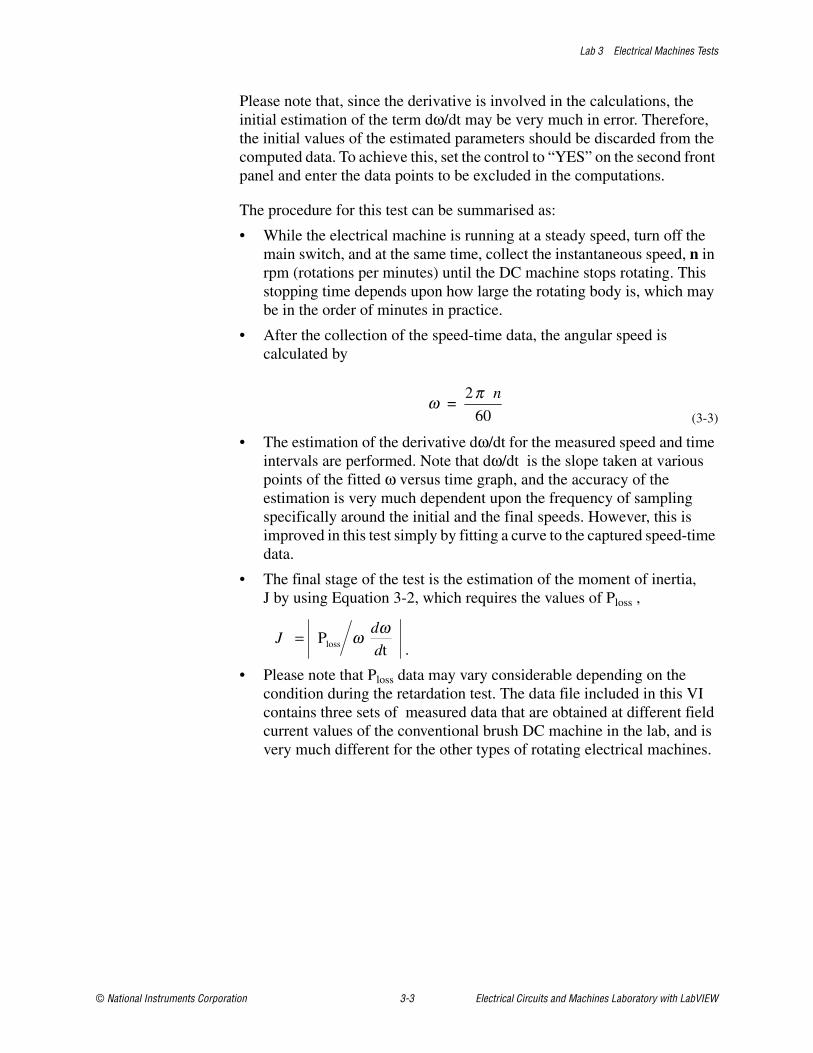
Lab 3 Electrical Machines Tests
© National Instruments Corporation 3-3 Electrical Circuits and Machines Laboratory with LabVIEW
Please note that, since the derivative is involved in the calculations, the initial estimation of the term dω/dt may be very much in error. Therefore, the initial values of the estimated parameters should be discarded from the computed data. To achieve this, set the control to “YES” on the second front panel and enter the data points to be excluded in the computations.
The procedure for this test can be summarised as:
• While the electrical machine is running at a steady speed, turn off the main switch, and at the same time, collect the instantaneous speed, n in rpm (rotations per minutes) until the DC machine stops rotating. This stopping time depends upon how large the rotating body is, which may be in the order of minutes in practice.
• After the collection of the speed-time data, the angular speed is calculated by
(3-3)
• The estimation of the derivative dω/dt for the measured speed and time intervals are performed. Note that dω/dt is the slope taken at various points of the fitted ω versus time graph, and the accuracy of the estimation is very much dependent upon the frequency of sampling specifically around the initial and the final speeds. However, this is improved in this test simply by fitting a curve to the captured speed-time data.
• The final stage of the test is the estimation of the moment of inertia, J by using Equation 3-2, which requires the values of Ploss ,
.
• Please note that Ploss data may vary considerable depending on the condition during the retardation test. The data file included in this VI contains three sets of measured data that are obtained at different field current values of the conventional brush DC machine in the lab, and is very much different for the other types of rotating electrical machines.
60
2 =
nπω
Jd
d P
t loss= ω ω

Lab 3 Electrical Machines Tests
Electrical Circuits and Machines Laboratory with LabVIEW 3-4 www.ni.com
Figure 3-1. The front panels of the retardation test, Retardation Test.vi and Calculated Inertia J.vi

Lab 3 Electrical Machines Tests
© National Instruments Corporation 3-5 Electrical Circuits and Machines Laboratory with LabVIEW
Figure 3-2. The explanations diagrams of the front panels, Retardation Test.vi and Calculated Inertia J.vi
After pressing "Get Speed" button, the simulated deceleration, speedversus time curve is displayed in this graph.
The coefficients of thetime axis and thestarting speed for thesimulation can be sethere.
This graph displays the estimatedangular speed versus timecharacteristic.
If the "Calculate dω/dt" button ispressed, this graph displays thecalculated values of dω/dt.
The fitted equation is given here.
The controls can be usedto define the method ofcurve fitting to thedeceleration curvedisplayed on the left. Usethe button to initiate thecurve fitting.
These are additionalcontrol buttons thatcan be used tocalculate dω/dt and J,or to restart the test.
When "Calculate J" button is activated, this front panel is opened. The graph displays the values ofthe moment of inertia point by point based upon the Ploss values stored in a text file.
Select the Ploss file to be used for thecalculation of J. Three separate files areincluded in this test. However, pleaseremember that Ploss file should be created byan additional test on the rotating machine.
Use the controlshere to eliminate thedata points thatlooks incorrrect.
Use this buttonto calculate themoment ofinertia.

Lab 3 Electrical Machines Tests
Electrical Circuits and Machines Laboratory with LabVIEW 3-6 www.ni.com
The specifications of the hardware usedThe devices used in this experiment have the following specifications.
Computer: Pentium PC , 32 MB RAM, and >1 GB hard disk,
Data acquisition system: National Instruments AT-MIO-16E-10 data acquisition card with 8 differential inputs, 12-bit resolution, 100 kHz sampling frequency, 2 Analog Outputs (for 12-bit D/A conversion), 8 Digital I/O.
The devices under test:In this test, the inertia of a rotating machine system is measured. In the system available, there are three medium-size electrical machines that are all coupled to the same shaft. The ratings of the electrical machines are given below:
Signal conditioning device:In this experiment, the real-time speed is measured by using a DC tacho-generator that is attached to the shaft of the machines.
Induction (Asynchronous) Motor
Educational ObjectivesAfter performing this experiment, students should be able to:
• Understand how the equivalent circuit parameters of a three-phase induction motor are determined.
• Study the behaviour of the motor and the motor characteristics under the sinusoidal steady-state operation, including the torque-speed characteristics at different supply frequencies and supply voltages.
Table 3-1. The Ratings of the Electrical Machines Used in the Laboratory
DC MachineSlip-ring Induction
MachineSynchronous
Machine
5.5 kW1250/1500 rpm220 V27.6 Ashunt field210 V0.647 A
415 V, Y, 3 ~11 A, 1410 rpm5.5 kWcos φ : 0.8550 HzROTOR: 170 V, Y, 22 A
8 kW415 V10.5 A1500 rpm50 Hz

Lab 3 Electrical Machines Tests
© National Instruments Corporation 3-7 Electrical Circuits and Machines Laboratory with LabVIEW
Reference Readings1. Electrical Machines, Drives, and Power Systems, T.Wildi, Prentice Hall,
1991.
2. N. Ertugrul, Electric Power Applications Lecture Notes, Department of Electrical and Electronic Engineering, University of Adelaide, 1997.
3. Electrical Machines and Drive Systems, C.B. Gray, Longman Scientific and Technical, Co publisher John Wiley & Sons, 1989.
Background InformationThe aim of this experiment is to identify the equivalent circuit parameters of a three-phase asynchronous machine and perform the analysis based upon the variable input and motor parameters.
Due to the limited space and very well known theory about such motors, the theory of the asynchronous motors will not be repeated here. Therefore, it is expected that the basic knowledge is obtained from the text books or any other resources prior to the tests.
The overall experiment is self-explanatory. The principal front panels of the test are given in Figures 3-3 to 3-9. Please remember that there are many other sub-sections in the VI, and each section includes a “theory” sub-vi, which provides a brief explanation about the issue under study.
Furthermore, please follow the logical order that is structured in the VI. However, as stated earlier, further study may be needed to understand the concepts presented in the sub-sections.

Lab 3 Electrical Machines Tests
Electrical Circuits and Machines Laboratory with LabVIEW 3-8 www.ni.com
Figure 3-3. The first front panel of the Induction Motor Experiment.vi.
Figure 3-4. The front panel showing the major sections in the experiment.

Lab 3 Electrical Machines Tests
© National Instruments Corporation 3-9 Electrical Circuits and Machines Laboratory with LabVIEW
Figure 3-5. The front panel of the Blocked Rotor Test.vi.
Figure 3-6. The front panel of the No-Load Test.vi.

Lab 3 Electrical Machines Tests
Electrical Circuits and Machines Laboratory with LabVIEW 3-10 www.ni.com
Figure 3-7. The front panel showing the major options in the Steady-State Performance Characteristics Section.
Figure 3-8. The front panel showing the sub-sections of the major options in the performance characteristic section.

Lab 3 Electrical Machines Tests
© National Instruments Corporation 3-11 Electrical Circuits and Machines Laboratory with LabVIEW
Figure 3-9. A sample front panel selected from the menu given in Figure 3-8.
The Specifications of the Hardware UsedThe devices used in this experiment have the following specifications.
Computer: Pentium PC , 32 MB RAM, and >1 GB hard disk,
Data acquisition system: National Instruments AT-MIO-16E-10 data acquisition card with 8 differential inputs, 12-bit resolution, 100 kHz sampling frequency, 2 Analog Outputs (with 12-bit D/A conversion), 8 Digital I/O.
The devices under test:This test is performed on a slip-ring asynchronous motor that has the ratings given in Table 3-1.
Signal conditioning devices:In this experiment, the voltage and the current measurements are achieved by using the identical signal conditioning devices that were given in Figure 2-4.
Other auxiliary instruments:Supply: 3-phase, 415V, 50 Hz

Lab 3 Electrical Machines Tests
Electrical Circuits and Machines Laboratory with LabVIEW 3-12 www.ni.com
WiringTo perform a real-time test, Figure 1 should be incorporated in the main vi, and the channels should be assigned as given below.
Channel 1 to the “Phase 1 voltage and Channel 2 to the Line 1 current.
The no-load and the blocked-rotor tests on the laboratory slip ring induction motor with the external resistance in the rotor circuit set to zero are performed, and Phase 1 voltage and Line 1 current are measured in real-time. The per-phase active power is calculated from the rms values of the current, the voltage and the phase angle that is determined from the real-time waveforms. The real-time circuit connection is given in Figure 3-10. In the Blocked-Rotor test, a reduction in the applied voltage is achieved by inserting resistances in series with the stator terminals of the motor as shown in Figure 3-10a. Figure 3-10b illustrates the wiring diagram of the No-load test.
Figure 3-10. The wiring diagrams for the tests.
Synchronisation of a Synchronous Generator
Educational ObjectivesAfter performing this experiment, students should be able to:
• Study the requirements for the “synchronisation of a three-phase synchronous generator”.
Vs1
Vs2
Vs3
ωωωωm = 0
N
to PC
Starting resistorsmust be short circuited
during the test.
Clampedrotor
StarconnectedSlip-ringInduction
Motor
Currentmeasurement
ase voltageasurement
to PC
Seriespower
resistors
DC Generatorfor loadingthe motor
Vs1
Vs2
Vs3
ωωωωm ~ ωωωωs(synchronous
speed)
N
Starting resistorsmust be short circuited
during the test.
Currentmeasurement
to PC
StarconnectedSlip-ringInduction
Motor
Phase voltagemeasurement
to PC
a b

Lab 3 Electrical Machines Tests
© National Instruments Corporation 3-13 Electrical Circuits and Machines Laboratory with LabVIEW
• Demonstrate the concept of “synchronisation” by observing the real-time voltage waveforms, three-phase voltage phasors (voltage vectors), and other estimated numerical values such as frequencies, phase angles.
Reference ReadingsFurther study may be necessary to have a deep understanding of “synchronisations” in the synchronous machines.
T.Wildi, Electrical Machines, Drives, and Power Systems, pp. Prentice Hall, 1991.
Background InformationSynchronous generators are usually operated in parallel. The number of parallel generators in an interconnected power system can be as high as hundreds. The principal purpose of this interconnection is the continuity of the service and the economy in plant investment and the operating cost. For example, since the power requirements of a large system vary during the day, generators are successively connected to the system or temporarily disconnected from the system to provide the demanded power.
A synchronous generator can be connected to an infinite bus (large power grid, the bus that has a constant voltage and frequency) by driving it at synchronous speed and adjusting its field current so that its terminal voltage is equal to that of the bus. In addition, if the frequency of the incoming generator is not exactly equal that of the bus, the phase relation between its voltage and the bus voltage will vary at a frequency equal to the difference between the frequencies of the two voltages. However, in a practical system the voltage differences may also occur due to other reasons. Therefore, there are more conditions that should be met before the generator is connected to the bus. The conditions for “synchronisation” are listed below:
1. Phase sequence of the generator must be same with the bus:
Phase 1 of the generator should be connected to Phase 1 of the bus
Phase 2 of the generator should be connected to Phase 2 of the bus
Phase 3 of the generator should be connected to Phase 3 of the bus
This condition depends on the initial wiring of the generator. Once the wiring is done there is no need to check this condition again. Either a special device or a three-phase induction motor can be used to check the phase sequence. In case of identical phase sequence, the motor should rotate in the same direction both when it is connected to the bus side and to the generator side.
2. The generator frequency must be equal to the bus frequency. In a balanced three-phase system, this condition can be observed by measuring the frequency of say Phase 1 voltages on both sides.

Lab 3 Electrical Machines Tests
Electrical Circuits and Machines Laboratory with LabVIEW 3-14 www.ni.com
3. The generator voltages should be equal to the corresponding bus voltages:
Phase 1 voltage of the generator should be equal to Phase 1 voltage of the bus
Phase 2 voltage of the generator should be equal to Phase 2 voltage of the bus
Phase 3 voltage of the generator should be equal to Phase 3 voltage of the bus
4. The generator voltages should be in phase with the corresponding bus voltages:
Vgen1 in phase with Vbus1
Vgen2 in phase with Vbus2
Vgen3 in phase with Vbus3
The Front Panel and the OperationTo resume the test, the test setup shown in Figure 3-11 should be prepared. Six parameters, three-phase bus voltages and three-phase generator voltages, should be measured.
Please note that, in a practical system, the input voltages (generator and bus voltages) can be as high as thousands of volts. Make sure that the high voltages are attenuated (and isolated) to a level (voltage sensors in the circuit) that can be directly connected to your DAQ card, and assigned (which may be changed in the diagram of the VI).
Channels 1,2 and 3 to the “Bus phase voltages 1,2 and 3” respectively
Channels 4,5 and 6 to the “Generator phase voltages 1,2 and 3” respectively
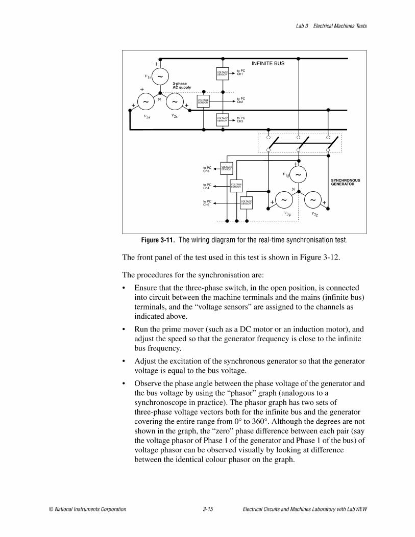
Lab 3 Electrical Machines Tests
© National Instruments Corporation 3-15 Electrical Circuits and Machines Laboratory with LabVIEW
Figure 3-11. The wiring diagram for the real-time synchronisation test.
The front panel of the test used in this test is shown in Figure 3-12.
The procedures for the synchronisation are:
• Ensure that the three-phase switch, in the open position, is connected into circuit between the machine terminals and the mains (infinite bus) terminals, and the “voltage sensors” are assigned to the channels as indicated above.
• Run the prime mover (such as a DC motor or an induction motor), and adjust the speed so that the generator frequency is close to the infinite bus frequency.
• Adjust the excitation of the synchronous generator so that the generator voltage is equal to the bus voltage.
• Observe the phase angle between the phase voltage of the generator and the bus voltage by using the “phasor” graph (analogous to a synchronoscope in practice). The phasor graph has two sets of three-phase voltage vectors both for the infinite bus and the generator covering the entire range from 0° to 360°. Although the degrees are not shown in the graph, the “zero” phase difference between each pair (say the voltage phasor of Phase 1 of the generator and Phase 1 of the bus) of voltage phasor can be observed visually by looking at difference between the identical colour phasor on the graph.
v1s
v3s v2s
+
~3-phaseAC supply+
~ +~+N
to PCCh1
VOLTAGESENSOR
to PCCh2
VOLTAGESENSOR
to PCCh3
VOLTAGESENSOR
v1g
v3g v2g
+
~
~ +~+
N
INFINITE BUS
SYNCHRONOUSGENERATOR
to PCCh5
VOLTAGESENSOR
to PCCh4
VOLTAGESENSOR
to PCCh6
VOLTAGESENSOR

Lab 3 Electrical Machines Tests
Electrical Circuits and Machines Laboratory with LabVIEW 3-16 www.ni.com
During the synchronisation process the three-phase phasors rotate slowly as it follows the phase angle between the generator and the bus voltages. If the generator frequency is slightly higher or lower than the bus frequency the direction of the phasor rotation is different (clockwise or counterclockwise).
• At the instant of synchronisation, when all of the four conditions listed in the Introduction section are met, the corresponding LED lights on the front panel turn into “green” and the new “switch” position and the “picture” indicate the correct instant for the synchronisation.
SUGGESTIONS: Because of potential wiring mistakes, wrong scaling factors, or imperfect or faulty signal conditioning devices, the Synchronisation.vi may produce a “wrong synchronisation instant”. Therefore, it is suggested that “Synchronisation Observer” should be used in an open-loop system first. More careful test set up may be prepared to close the loop, simply by connecting the “MAIN SWITCH” output on the front panel to a digital output line, which may control the actual power switch automatically. It should be reminded here that an additional signal conditioning circuit (containing an opto-coupler and a static relay) is required to interface the main switch with the digital output of the DAQ card. To study the synchronisation:
• Operate the synchronous machine
• Run Synchronisation.vi
• Press the “START ACQUISITION” button to start the data acquisition
• After you obtain the synchronisation conditions, you may stop the acquisition and print out the front panel for further analysis.

Lab 3 Electrical Machines Tests
© National Instruments Corporation 3-17 Electrical Circuits and Machines Laboratory with LabVIEW
Figure 3-12. Front panel of the synchronisation test and the explanations panel
This graph displays the three-phase supply (infinite-bus)voltages in real-time. Thevoltage data is updatedregularly.
The three-phase bus and thegenerator voltage phasors aredisplayed in this graph. Refer to thelegend of the graph to determine thecorresponding supply and thegenerator voltage phasors.
This graph displays the three-phase generator voltages in real-time. The voltage data is updatedsimultaneously with the busvoltage data.
The current status of each of thesynchronisation condition isdisplayed here by the LEDindicators.
At the instant of the"synchronisation", all LEDs becomeGREEN and the main switchchanges the position.
This pictureringanimatestheOperatingModes :(openswitch/closeswitch)
The numericalvalues of thefrequencies ofthe bus voltageand generatorvoltage, phaseangles, and rmsvalues of thebus and thegeneratorvoltages arecalculated andindicated herefor anadditionalconfirmation.

Lab 3 Electrical Machines Tests
Electrical Circuits and Machines Laboratory with LabVIEW 3-18 www.ni.com
The Specifications of the Hardware UsedThe devices used in this experiment have the following specifications.
Computer: Pentium PC , 32 MB RAM, and >1 GB hard disk,
Data acquisition system: National Instruments AT-MIO-16E-10 data acquisition card with 8 differential inputs, 12-bit resolution, 100 kHz sampling frequency, 2 Analog Outputs (for 12-bit D/A conversion), 8 Digital I/O.
The devices under test:This test is performed on a synchronous motor that has the ratings given previously in Table 3-1.
Signal conditioning devices:In this experiment, the voltage and the current measurements are achieved by using the identical signal conditioning devices that were shown in Figure 2-4.
Other auxiliary instruments:Supply: 3-phase, 415V, 50 Hz

© National Instruments Corporation 4-1 Electrical Circuits and Machines Laboratory with LabVIEW
Lab 4Dynamic Simulation of Electrical Motors
Dynamic behaviour of the electric motors is a difficult topic to study unless a computer-aided tool is used, or an experimental system is implemented together with specific measuring devices in a laboratory environment.
Three simulation tools are provided in this section, which are designed to investigate the dynamic behaviour of the three commonly used electric motors: three-phase asynchronous motor, three-phase brushless permanent magnet synchronous motors and separately excited step-down converter driven DC motors.
These simulation tools can produce results for any given parameter. Therefore, the correct settings of the inputs are very crucial for meaningful outputs. In addition, the interpretation of the results and the deep understanding of the methods heavily depend upon the background knowledge of the user about the machine.
Induction (Asynchronous) Motor Simulation
Educational ObjectivesAfter performing this experiment, students should be able to:
• Understand the dynamic behaviour of the three-phase induction motors under no-load or load conditions.
• Observe the starting performance of the motor.
Reference ReadingsThe reference book given below was used to derive the motor’s equations in d-q reference frame and to obtain the inverse transformations.
P.C. Krause, Analysis of Electrical Machinery, McGraw-Hill, 1987.

Lab 4 Dynamic Simulation of Electrical Motors
Electrical Circuits and Machines Laboratory with LabVIEW 4-2 www.ni.com
Background InformationThe VI named “Induction motor simulation.vi” is provided in this section, which can be used to investigate the dynamic operation of the three-phase asynchronous motors. In the simulation, the asynchronous motor is powered from a three-phase sinusoidal voltage source and the motor is started from standstill.
In the VI, the motor is modelled in the d-q reference frame by five non-linear differential equations, and the simulation uses the stationary reference frame of the induction motor as explained in the reference given above.
In the simulation, the fluxes are selected as the state space variables. The non-linear differential equations are given below.
(4-1)
(4-2)
(4-3)
(4-4)
(4-5)
Where, D = , p is the number of poles of the motor, J is the moment of inertia, ωb is the base speed in rad/s, subscripts d and q represents the d and q axis, and subscripts s and r indicates the stator and rotor quantities. The electromagnetic torque developed by the machine is given as
(4-6)
++++−−−−
′′′′−−−−==== qr
msds
bqs
rrsqsb
qs
D
XR
D
XRv
dt
dψψψψψψψψ
ωωωωωωωωψψψψωωωω
ψψψψ
++++
′′′′−−−−++++==== dr
msds
rrsqs
bdsb
ds
D
XR
D
XRv
dt
dψψψψψψψψψψψψ
ωωωωωωωωωωωω
ψψψψ
−−−−−−−−′′′′
−−−−′′′′
++++==== drb
rqr
ssrqs
mrqrb
qr
D
XR
D
XRv
dt
dψψψψ
ωωωωωωωωωωωωψψψψψψψψωωωω
ψψψψ
′′′′−−−−
−−−−++++′′′′
++++==== drssr
qrb
rds
mrdrb
dr
D
XR
D
XRv
dt
dψψψψψψψψ
ωωωωωωωωωωωωψψψψωωωω
ψψψψ
(((( ))))
−−−−====
Jp
TTdt
dLe
r 12
ωωωω
2mrrss XXX −−−−′′′′
(((( ))))dsqrdrqsb
me D
XpT ψψψψψψψψψψψψψψψψ
ωωωω−−−−
====
223

Lab 4 Dynamic Simulation of Electrical Motors
© National Instruments Corporation 4-3 Electrical Circuits and Machines Laboratory with LabVIEW
The above differential equations are solved by Runge-Kutta numerical method that is implemented using the tools available in LabVIEW. The Runge-Kutta method does not need a special starting arrangement, the step width can be changed easily and storage requirement is minimal. The Runge-Kutta formula used in the numerical solution involves weighted
average values taken at different points in the interval , and is given by
(4-7)
Where the coefficients
k1 = ∆t f’(xn , yn)
k2 = ∆t f’(xn + ∆t/2 , yn + k1/2)
k3 = ∆t f’(xn + ∆t/2 , yn + k2/2)
k4 = ∆t f’(xn + ∆t , yn + k3)
Here n is the time step, ∆t = tn+1 - tn , f’(xn , yn) = dyn/d xn .
The simulation also provides an inverse transformation to determine the abc reference frame which corresponds to the real parameters of the motor for easy comparison.
Conversion to abc reference frame is achieved by using the below transformations.
(4-8)
where fabcs = [fas fbs fcs]T and fqdos = [fqs fds fos]T.
Here, f can be either the voltage, the current, or the flux linkage of the machine.
(4-9)
In the above formula, θ = is used for the stator transformation, and
θ= is used for the rotor transformations.
1++++≤≤≤≤≤≤≤≤ nn ttt
yn+1 = yn + (k1 + 2 k2 + 2 k3 + k4) / 6
fabcs = (K-1)* fqdos
( ) ( )( ) ( )
++−−=−
13/2sin3/2cos
13/2sin3/2cos
1sincos1
πθπθπθπθ
θθK
∫ dtω
( )∫ − dtrωω
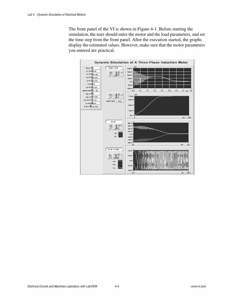
Lab 4 Dynamic Simulation of Electrical Motors
Electrical Circuits and Machines Laboratory with LabVIEW 4-4 www.ni.com
The front panel of the VI is shown in Figure 4-1. Before starting the simulation, the user should enter the motor and the load parameters, and set the time step from the front panel. After the execution started, the graphs display the estimated values. However, make sure that the motor parameters you entered are practical.

Lab 4 Dynamic Simulation of Electrical Motors
© National Instruments Corporation 4-5 Electrical Circuits and Machines Laboratory with LabVIEW
Figure 4-1. The front panel of Induction motor simulation.vi and the explanations diagram.
Tasks to Study• You can start the simulation by using the default values of the motor
parameters. Additional motor parameters can be obtained from the reference book given above or from any other Electrical Machines related text book. In addition, the motor parameters can be determined experimentally as studied in Lab 3.
• Run the simulation and observe the changes in the electromagnetic torque, the speed, and the line currents.
• Vary the total moment of inertia and the load torque (only one at a time) and observe the changes on the speed-time characteristic.
• Vary the equivalent rotor resistance of the motor and observe the changes on the torque-speed characteristics.
• The electromagnetic torque can be plotted in two different forms: torque versus speed and torque versus slip. Run the simulation until the steady-state speed is reached and comment on the above characteristics.
• Have you noticed any changes on the value of the slip when the load (or the equivalent rotor resistance or the moment of inertia) is increased?
Enter themotor andloadparametershere.
Use the pull-downcontrols todisplay thedesiredsimulatedmotorparameters onthe graphgiven on theright handside.
Electromagnetic torque versus speed andelectromagnetic torque versus time graphs aredisplayed here.
The instantaneous speed-time characteristic isshown in this graph.
Direct and quadrature axis instantaneouscurrents of the motor are shown here.
This graph illustrates the above currentwaveforms in the abc reference frame (afterthe inverse transformation).
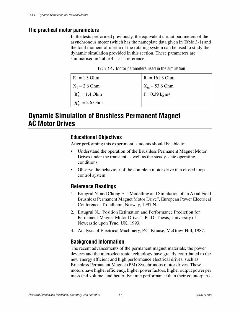
Lab 4 Dynamic Simulation of Electrical Motors
Electrical Circuits and Machines Laboratory with LabVIEW 4-6 www.ni.com
The practical motor parametersIn the tests performed previously, the equivalent circuit parameters of the asynchronous motor (which has the nameplate data given in Table 3-1) and the total moment of inertia of the rotating system can be used to study the dynamic simulation provided in this section. These parameters are summarised in Table 4-1 as a reference.
Dynamic Simulation of Brushless Permanent Magnet AC Motor Drives
Educational ObjectivesAfter performing this experiment, students should be able to:
• Understand the operation of the Brushless Permanent Magnet Motor Drives under the transient as well as the steady-state operating conditions.
• Observe the behaviour of the complete motor drive in a closed loop control system
Reference Readings1. Ertugrul N. and Chong E., “Modelling and Simulation of an Axial Field
Brushless Permanent Magnet Motor Drive”, European Power Electrical Conference, Trondheim, Norway, 1997.N.
2. Ertugrul N.,“Position Estimation and Performance Prediction for Permanent-Magnet Motor Drives”, Ph.D. Thesis, University of Newcastle upon Tyne, UK, 1993.
3. Analysis of Electrical Machinery, P.C. Krause, McGraw-Hill, 1987.
Background InformationThe recent advancements of the permanent magnet materials, the power devices and the microelectronic technology have greatly contributed to the new energy efficient and high performance electrical drives, such as Brushless Permanent Magnet (PM) Synchronous motor drives. These motors have higher efficiency, higher power factors, higher output power per mass and volume, and better dynamic performance than their counterparts.
Table 4-1. Motor parameters used in the simulation
R1 = 1.3 Ohm
X1 = 2.6 Ohm
= 1.4 Ohm
= 2.6 Ohm
Rc = 161.3 Ohm
Xm = 53.6 Ohm
J = 0.39 kgm22R′′′′
2X′′′′

Lab 4 Dynamic Simulation of Electrical Motors
© National Instruments Corporation 4-7 Electrical Circuits and Machines Laboratory with LabVIEW
Such motors can be broadly classified into two groups. The first group possesses trapezoidal back EMFs and is called Brushless Trapezoidal Permanent Magnet (BTPM) Motors (or simply brushless DC motors). The second group possesses sinusoidal back EMFs and is called Brushless Sinusoidal Permanent Magnet (BSPM) motors (or as brushless permanent magnet synchronous motors). In order to produce a constant ripple-free electromagnetic torque, both types require rectangular or sinusoidal winding currents respectively. However, any other current excitation is possible considering the electromagnetic torque will have ripples.
A very flexible computer simulation tool is provided here. This tool can be used to study the motor behaviour and to analyse the complete drive system (including the inverter and the controller) without implementing the hardware. In addition to this, the drive simulations can be forced to operate under the extreme conditions without damaging the motor drive. In the simulation, the dynamic as well as the steady-state operation of the three-phase permanent magnet AC motor drive can be performed in a variety of operating conditions, such as with and without current control, with sinusoidal or rectangular current excitation, and with sinusoidal or trapezoidal back EMF waveforms.
In order to obtain a general dynamic model for the motor drive, the three-phase abc modelling approach is used, and the differential equations of the motor drive were solved simultaneously. Figure 4-2 illustrates the block diagram of the complete drive.
Figure 4-2. The block diagram of the Brushless PM Motor Drive
The voltage equations of the motor in the matrix form are expressed as:
(4-10)
SpeedControllerBack EMFgenerator
3 PhaseInverter
Brushless PMmotor
CurrentController
Positionsensor
+
+
=
3
2
1
3
2
1
3
2
1
3
2
1
00
00
00
00
00
00
v
v
v
e
e
e
i
i
i
dt
d
L
L
L
i
i
i
R
R
R

Lab 4 Dynamic Simulation of Electrical Motors
Electrical Circuits and Machines Laboratory with LabVIEW 4-8 www.ni.com
Here v1, v2, and v3 are the phase voltages of the motor; R is the winding resistance; i1, i2, and i3 are the line currents; L is the equivalent winding inductance; and e1, e2, and e3 are the back EMFs.
The electromagnetic torque, Te and the mechanical equation of the motor are given by
(4-11)
(4-12)
Where is the angular speed; is the load torque; J is the inertia.
Assuming the three-phase stator windings are symmetrically displaced 120° electrical angle, the back EMF equations of the BSPM motor is represented as:
(4-13)
For the BTPM motors, however, the back EMF of one phase is given in the piecewise linear form as:
(4-14)
Where is the maximum value of the back emf, is back EMF
constant, and is the electrical rotor position, and they are expressed as
(4-15)
( )332211
1ieieieT
re ++=
ω
dt
dJTT r
le
ω=−
rωlT
−−=
)34sin(
)32sin(
)sin(
3
2
1
πθπθ
θ
em
em
em
E
E
E
e
e
e
≤<−
≤<−
≤<−−
≤<
≤<
=
πθππθπ
πθπ
πθππθπ
πθπ
πθθπ
26
11)2(
6
611
67
67
65
)(6
65
6
60
6
eem
em
eem
em
eem
E
E
E
E
E
e
mE ek
eθ
rem kE ω=

Lab 4 Dynamic Simulation of Electrical Motors
© National Instruments Corporation 4-9 Electrical Circuits and Machines Laboratory with LabVIEW
(4-16)
Where, is the mechanical rotor position; and is the number of pole pair.
The BSPM and BTPM motors are fed from a three-phase rectifier/inverter circuit. The motor drive simulation provided in this courseware include the inverter states that are determined from the estimated parameters given in the table below.
The VI in this test is named Brushless PM motor simulation.vi. The front panels of the simulation are given in Figure 4-3 below. Two front panels are constructed in this test due to the intensive calculations and multiple number outputs on the motor drive. In addition, small control boxes were included to display the multiple parameters on the same graph for comparison purposes, such as the three phase line currents and the phase voltages.
Table 4-2. Summary equations for the estimation of the star point voltage and the phase voltages
TRAPEZOIDAL BACK EMFs SINUSOIDAL BACK EMFs
e1 + e2 + e3 ≠ 0(except zero crossing instants)
e1 + e2 + e3 = 0
va, vb, vc = ± Vdc / 2
vs = K [(va + vb + vc) - (e1 + e2 + e3)]
If i1 = 0 K = 1/2 then v1 = e1 , v2 = vb - vs , v3 = vc - vs
If i2 = 0 K = 1/2 then v1 = va - vs , v2 = e2 , v3 = vc - vs
If i3 = 0 K = 1/2 then v1 = va - vs , v2 = vb - vs , v3 = e3
If i1≠ 0 , i2 ≠ 0 , i3 ≠ 0K = 1/3 then v1 = va - vs , v2 = vb - vs , v3 = vc - vs
∫== dtpp rre ωθθ
rθ p
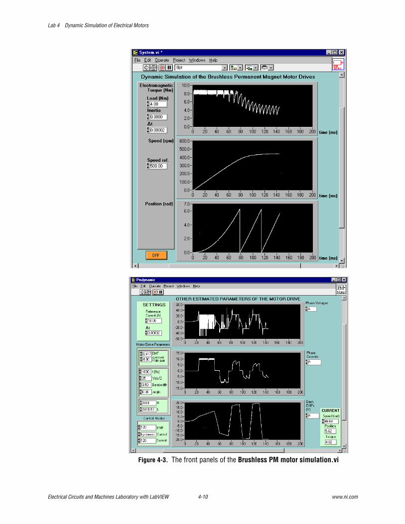
Lab 4 Dynamic Simulation of Electrical Motors
Electrical Circuits and Machines Laboratory with LabVIEW 4-10 www.ni.com
Figure 4-3. The front panels of the Brushless PM motor simulation.vi

Lab 4 Dynamic Simulation of Electrical Motors
© National Instruments Corporation 4-11 Electrical Circuits and Machines Laboratory with LabVIEW
Figure 4-4. The explanations windows for the front panels given in Figure 4-3.
The settingsfor the loadtorque, themoment ofinertia and thefix time stepfor the Runge-Kuttaintegrationmethod can beentered here.
The desiredspeed(referencespeed) in rpmcan also be set.
Total electromagnetic torque versus time graph is shown here
The speed versus time graph is shown here
The instantaneous electrical rotor position in radians versustime graph is shown here
Use thisbutton to stopthe simulation.
Input thereferencecurrentamplitudehere.
The phase voltage(s) of the motor is shownhere. Select the phase or the phases from thecontrol given on right side of the graph.
Input themotor anddriveparametershere.
Type of thebrushless PMmotor andshape of thecontrolledcurrent canbe set here.
The phase current(s) of the motor is displayedhere. Select the phase or the phases from thecontrol given on right side of the graph.
The phase back emf waveform(s) of the motoris displayed here. Select the phase or the phasesfrom the control given on right side of thegraph.
The currentspeed inradian/s ,rotor positionand torque isindicatedhere.

Lab 4 Dynamic Simulation of Electrical Motors
Electrical Circuits and Machines Laboratory with LabVIEW 4-12 www.ni.com
Tasks to Study• You can start the simulation by using the default values of the motor
parameters. Different motor parameters can be obtained from the many other text book or from the motor manufacturers’ catalogues. Please note that the motor and the controller settings are given in the second front panel.
• Run the simulation and observe the changes in the total electromagnetic torque, the speed, and the rotor position, and identify the acceleration time of the motor.
• Vary the total moment of inertia and/or the load torque and observe the changes on the speed-time characteristic.
• For the above operating conditions, observe the phase voltages, the line currents and the back emf waveforms of the motor by swapping between the two front panels provided.
• Study the transient behaviour of the motor drive for the different motor types (sinusoidal and trapeziodal brushless PM motors) and for the different current controller settings (hysteresis and PWM current control), which can be altered from the second front panel.
The practical motor parametersThis test is performed on a brushless Permanent Magnet motor. Table 4-3 provides a set of motor parameters that are measured from a practical motor, which can be used to study the simulation of the motor drive.
Direct Current (DC) Motor Drive Simulation
Educational ObjectivesAfter performing this experiment, students should be able to:
• Understand the operation of a DC motor under the transients as well as the steady-state operating conditions.
Table 4-3. The practical motor parameters that can be used in the simulation
Torque constant 0.31 Nm/A
Back emf constant, ke 0.417 V/rad/s
Moment of inertia, J 0.0008 kgm2
Number of poles 8
Winding resistance, R 0.8 Ohm
Equivalent winding inductance, L 3.12 mH

Lab 4 Dynamic Simulation of Electrical Motors
© National Instruments Corporation 4-13 Electrical Circuits and Machines Laboratory with LabVIEW
• Observe the behaviour of the DC motor drive when it is excited from a simple Power Electronics Step-down DC-DC converter.
Reference Readings1. Electrical Machines and Drive Systems, C.B. Gray, Longman Scientific
and Technical, Co publisher John Wiley & Sons, 1989.
2. Electric Motors and Their Controls, An Introduction, T. Kenjo, Oxford Science Publications, Oxford University Press, 1991.
Background InformationIn industrial drives containing DC motors, starting, braking, speed and load changing commonly occur. To predict and understand the operation of the DC motor drives (Motor + Power Electronics controller) under these transient conditions, either a real motor drive should be built, or the dynamic equations of the motor should be solved numerically in a computer by using the simulation model of the drive.
However, building the real motor drive is an expensive solution. In addition to this, the real system cannot easily imitate the potential faults that might occur in the real world. One of the solutions to this problem is to model the drive system and analyse it using LabVIEW. If the simulation tool is carefully designed, the information obtained from the simulation can be used to determine the behaviour of the motor under transient operating conditions. Moreover, the simulation results may help the user to determine the ratings of the drive, nature and type of its controller, and the settings of the protective devices.
In the VI named “DC motor simulation.vi”, a Permanent Magnet excited (constant winding excitation) DC motor drive simulation is provided. The motor is powered from a step-down DC-DC converter as shown in the figure on the front panel.
In the simulation, the following equations are used: the voltage equation of the armature circuit, the dynamic equation of the motor-load (mechanical) system, and the electromagnetic torque equation respectively.
(4-17)
(4-18)
(4-19)
aa
aaaa edt
diLiRv ++=
Lmm
a TBdt
dJT ++= ωω
Te = ke ia

Lab 4 Dynamic Simulation of Electrical Motors
Electrical Circuits and Machines Laboratory with LabVIEW 4-14 www.ni.com
Where, va is the supply voltage, ia is the winding current , Ra is the resistance of the armature circuit, La is the inductance of the armature circuit, J is the moment of inertia of the system (including the motor and the load), the back emf is ea = ke.ω.ω.ω.ωm (here ke is known as back emf constant or torque constant), ω, ω, ω, ωm is the angular speed of the system, Te is the electromagnetic torque developed by the motor, TL is the load torque, and B is the damping coefficient which is usually ignored.
Note that, the above voltage and the load equations are valid for any type of DC motor. In this work, a Permanent Magnet excited DC motor is considered, and the state variables ia and ωωωωm in the linear differential equations are solved simultaneously in LabVIEW by using the Runge-Kutta method available LabVIEW. The DC-DC converter was implemented to provide a PWM voltage waveform to the motor winding, which operates in open-loop. The duty cycles of the PWM signal can be varied by the controls provided on the front panel. The view of the Front Panel used in this VI is shown below.
It should be noted here that the motor drive implemented in this test is an open-loop system. This means that there is no speed or a current feedback in the drive. However, a closed-loop system can be achieved easily as it is implemented in the previous simulation tool (Brushless Permanent Magnet Motor Drive simulation).
The PWM signal generated in this VI controls the switching states of the transistor (Figure 4-5). The user can change the frequency as well as the duty cycle of the control signal from the front panel. The front panel of the VI is given in Figure 4-6.
Figure 4-5. Frequency modulated (FM) or Pulse Width Modulated (PWM) control signal
Period, T = 1/f
ONTIME,TON
OFFTIME,TOFF
100%T
TCycleDuty on=

Lab 4 Dynamic Simulation of Electrical Motors
© National Instruments Corporation 4-15 Electrical Circuits and Machines Laboratory with LabVIEW
Figure 4-6. The front panel of the DC motor drive simulation, DC motor simulation.vi, and the explanation windows.
Enter the mechanicalside parameters here.
Input thefrequency andthe duty cycleof the controlsignal here.
This graph displays the parameters based on theselection done by using the controls given below.When the "pu" (per-unit) switch is selected, anothercontrol appears next to the parameter's switchwhere the desired base value can be set.
This figure illustrates the complete circuitunder investigation. Use the controls to setthe supply and the DC motor parameters. Use this button to select the time base graphs or
the torque/speed characteristic graph.
Use these switches to hide, to show, or to changethe base value of the estimated values in thesimulation.Pause, Start
and Stopbuttons aregiven here.
This animates therotation of themotor. The speedof the animation isproportional to thespeed of the motor.

Lab 4 Dynamic Simulation of Electrical Motors
Electrical Circuits and Machines Laboratory with LabVIEW 4-16 www.ni.com
Tasks to Study• Investigate the motor’s starting behaviour from stand still with and
without a mechanical load attached. Observe that the motor starts only after its developed torque exceeds the load torque and the acceleration rate depends upon the inertia of the system.
• When the motor is started, the initial value of the current and the back emf are zero. Due to the inductance of the circuit, the current rises and falls exponentially within the control interval of the converter's switch (the transistor). Vary the duty cycle and the frequency of the control signal and obtain the continuous and the discontinuous current conduction modes in the motor drive.
• Investigate how the motor current, the torque and the speed varies under the above operating conditions.
• You can observe CCW rotation by reversing the supply voltage.
• The motor and the system parameters can be varied at any instant time while the simulation is running. Vary only one parameter at a time and observe the estimated parameters.
• To study the retardation test, simply change the value of the supply voltage to zero when the duty cycle is 0%.
• The starting behaviour of the DC motor powered from a constant voltage source can be observed by keeping the transistor on all the time (by setting the duty cycle to 100%) at start. Repeat this test by reducing the duty cycle and observe the maximum current value obtained and the time taken to reach the steady state speed.
Additional References1. N. Ertugrul, New Era in Engineering Experiments: An Integrated
Interactive Teaching/ Learning Approach and Real Time Visualisations, International Journal of Engineering Education, Vol.14, No.5, pp. 344-355, 1998.
2. N. Ertugrul, A. P. Parker, and M. J. Gibbard, Interactive Computer-Based Electrical Machines and Drives Tests in the Undergraduate Laboratory at The University of Adelaide, EPE’97, 7th European Conference on Power Electronics and Application, Trondheim, Norway, 8-10 September 1997.
3. N. Ertugrul, Towards Virtual Laboratories: A Survey of LabView-Based Teaching/Learning Tools and Future Trends, The Special Issue on Applications of LabView in Engineering Education, International Journal of Engineering Education, No. 16, Vol.2, 2000.

© National Instruments Corporation A-1 Electrical Circuits and Machines Laboratory with LabVIEW
Appendix ALayout of the Laboratory and the Details of the Instrumentation
It is clear that changes in the laboratory practices are necessary because many of the things that we are doing can be done better with the help of technology. Although the initial cost may be high, if a right technology is selected continuous improvement can be achieved with a minimal cost. The cost of the development of such laboratories may be reduced further if the portion of the existing hardware is utilised and integrated with the existing system. Furthermore, the selection criteria of suitable software and the hardware are the major issue, which should have a long life-cycle, easy interface with the hardware products, and be compatible with the existing development tools.
The VIs provided here are implemented by using LabVIEW 5.0, and performed in the Electrical Machines and Drives Laboratory at the University of Adelaide. In the following paragraphs, this laboratory development project will be summarised briefly and some of the hardware details will be given to provide a background information for potential developers.
In laboratory applications, from the technical point of view, all the engineering problems deal with some physical quantities such as temperature, speed, position, current, voltage, pressure, force, torque, etc. A computer equipped with the suitable interface circuits, data acquisition systems and software, can give a visual look to these quantities, and can process the acquired data. These experiences can also be made available to the remote area user via Internet link using Internet Developers’ Toolkit of LabVIEW. Depending upon the target aim, the experimental system may contain many interfaces and many I/Os. Therefore, before the implementation, the final aim of the teaching/learning technology should be identified to determine the sub-units required.

Appendix A Layout of the Laboratory and the Details of the Instrumentation
Electrical Circuits and Machines Laboratory with LabVIEW A-2 www.ni.com
The photo of the laboratory is given in Figure A-1, which illustrates the current layout and frames only 8 of the 10 workstations. In this laboratory project, we took the old laboratory with the traditional switchboard, analog measuring devices and the electrical machines and equipped the lab with the computers, interface units and custom-written VIs. However, this task involved various design works and wiring works.
Figure A-1. The layout of the Electrical Machines and Drives Teaching Laboratory
The system diagram of the computer-assisted real-time experimental modules used in the laboratory is shown in Figure A-2.
Figure A-2. The system diagram of the computer-assisted laboratory
��������������
INTERFACE MODULE: Signal conditioning,transducers, isolation
Networkedprinters
Workstation 1
��������������������
����������������������������������������
����������������������������������������������������
������������������������������������������������������
DC machine
������������������������������������������������
Asysnchronousmotor
Synchronousmachine
Static devices
����������������
AT-MIO-16E-10
Remote area user
Camera
Interface fordigital I/O
����������������������������������������������

Appendix A Layout of the Laboratory and the Details of the Instrumentation
© National Instruments Corporation A-3 Electrical Circuits and Machines Laboratory with LabVIEW
In the laboratory, there are 10 Pentium-based PCs running Windows NT and LabVIEW 5.0 full development system, 2 Laser printers networked to the computers, 10 custom-built torque transducers to measure the instantaneous shaft torque in the machines (up to 50Nm), 120 custom-built current transducers (50A, and 100 A, DC to 100 kHz), 120 custom-built voltage isolation amplifiers (1000V rms, 50 kHz), 10 benches and switchboards, 10 static starting circuits and interfaces for the slip-ring induction motors, and wiring.
Each workstation in the laboratory contains identical, medium-power, mechanically-coupled rotating electrical machines: DC machine, slip-ring induction motor and synchronous machine. Table A-1 indicates the rated values of these machines. The measurement of shaft speed is achieved by an AC tachogenerator that is also attached to the common shaft.
The static devices for the test are supplied on the bench where interface terminals are available via custom-built voltage and current transducers. The accompanying hardware is highly flexible and includes suitable control signals for emergency shut down and control. A Logitech Video Camera has also been added to this system for the visual communication during remote area experimenting in future.
Every experiment in the laboratory requires some signals to be measured on specific channels. In the system designed, a maximum of eight parameters can be measured in real-time. The number eight was determined by the maximum number of parameters to be measured to perform the most complex experiment in the laboratory, such as three phase voltages, three line currents, speed and torque.
National Instruments’ AT-MIO-16E-10 data acquisition card is used in each workstation to perform the tests, which has the following specifications: 8 differential analog inputs, 12-bit resolution, 100 kHz sampling frequency, 2 Analog Outputs (for 12-bit D/A conversion), 8 Digital I/O.
Table A-1. The ratings of the electrical machines used in the laboratory
DC MachineSlip-Ring Induction
MachineSynchronous
Machine
5.5 kW1250/1500 rpm220 V27.6 Ashunt field210 V0.647 A
415 V, Y, 3 ~11 A, 1410 rpm5.5 kWcos f : 0.8550 HzROTOR: 170 V, Y, 22 A
8 kW415 V10.5 A1500 rpm50 Hz

Appendix A Layout of the Laboratory and the Details of the Instrumentation
Electrical Circuits and Machines Laboratory with LabVIEW A-4 www.ni.com
As mentioned above, each workstation accommodates a number of transducers that are used to measure high voltages and currents even at high switching frequencies. Noise immunity and personal safety are always an issue in such systems. Therefore, the workstations are designed to achieve total isolation. Firstly, the voltage dividers are used to attenuate the high voltages. The attenuated voltages are then isolated by using isolation amplifiers. Each isolation amplifier is also powered from a separate DC/DC converter. Each group of three transducers is equipped with separate floating power supplies for additional safety. The voltage transducers’ boards are also physically guarded against potential danger which may occur due to an arc.
In order to create a buffering circuit and to take full advantage of the resolution of the A/D conversion, additional amplifiers are used to amplify the signals obtained via the Hall-effect current transducers and the isolation amplifiers. The amplified signals are transferred to BNC terminal panels via coaxial cables to eliminate unwanted signals. All the transducers used in the laboratory are in-house custom-built. The principal circuit diagram of the transducers (voltage, current and torque) and the photos of the current and voltage transducers are shown in Figure A-3.
Considerable saving is achieved in this part of the project. It should be reported here that the overall cost of the transducers developed here was about one tenth of the equivalent system that is available commercially.
24 of these transducers (12 current and 12 voltage transducers) are housed inside a box that is located behind the main switchboard. They are permanently wired to the switchboard. The main switchboard and the transducers’ box are shown in Figure A-4.

Appendix A Layout of the Laboratory and the Details of the Instrumentation
© National Instruments Corporation A-5 Electrical Circuits and Machines Laboratory with LabVIEW
Figure A-3. The block diagrams of the custom-built transducers and the photos of the custom-built current and voltage transducers (three transducers on each card).
Figure A-4. The main switchboard and the transducers' box with BNC outputs.
DC/DCCONVERTER
+12V to
VOLTAGEREGULATOR
(±15V)
VOLTAGEREGULATOR
(+12V)
Voltage Attenuator
HighVoltage
Input
FUSE
~ 240V~ 240V
R2
R1
AD711IsolationAmpl.
ISO122P
BNCoutput
~ 240V
0
0 -+
BNC output to DAQ(voltage proportional
to torque)
Rotating PCBcontainingthe amplifierand
Slip-rings
Straingauges Steel
shaft
VOLTAGEREGULATOR
(±15V)
DEMODULATOR
~ 240V
VOLTAGEREGULATOR
(±15V)
Rm
AD711
M0
-+
BNCoutput
+
0-+
LA50-S
Voltage transducer Current transducer Torque transducer

Appendix A Layout of the Laboratory and the Details of the Instrumentation
Electrical Circuits and Machines Laboratory with LabVIEW A-6 www.ni.com
Associated with each machine set there is a switchboard panel which houses a collection of DC and AC meters, an analogue speed indicator and an analogue wattmeter. In the new computer-based method, these instruments are used as indicators only for additional checking and/or confirmation of the calculations, which are done via LabVIEW. Power electronic converters, single-phase transformers and other electromechanical devices are supplied separately on the test bench associated with the main switchboard of each machine set.
Four principal modifications were also done in the laboratory. These works include the interface development for the AC tachogenerators (Figure A-5a); the modification of the switchboards to accommodate the mains switches for the PCs, the interface boxes and the terminals of the additional current and voltage transducers for the static devices (Figure A-5b); the development of the tables for the PCs and the main BNC connector boards for easy I/Os (Figures A-5c and A-5d).
As mentioned before, the transducers are permanently wired to the main switchboard, and their outputs are made available on the BNC connector board that is shown in Figure A-5d. The user can select and assign any measurable signal to the Analog Inputs of the DAQ card on this board by using a two-end BNC cables as demonstrated in the figure.
Table A-2 summarises the ratings of the associated devices available in the laboratory.

Appendix A Layout of the Laboratory and the Details of the Instrumentation
© National Instruments Corporation A-7 Electrical Circuits and Machines Laboratory with LabVIEW
Figure A-5. The major modifications done in the laboratory.
Table A-2. The devices and their ratings available in the laboratory
Devices Ratings
3 phase supply 415V, 50 Hz, 50A
DC supply 200V, 40 A
Single phase auto transformers (as variable voltage sources)
240V, 8A, 50Hz
3-phase auto transformers Input: 415V , 15A Output: 0-470V
Pentium PCs 32 MB RAM, >1 GB
AT-MIO-16E-10 DAQ card from NI 8 diff. inputs, 12-bit, 100 kHz sampling frequency, 2 D/A (12-bit), 8 Digital I/O.
Rheostats 50 Ohm, 5 A
Capacitors 4µF, 1000V
dc
ba

Appendix A Layout of the Laboratory and the Details of the Instrumentation
Electrical Circuits and Machines Laboratory with LabVIEW A-8 www.ni.com
4 sets of mobile Special Electrical Machines set each containing: a 3-phase brushless PM motor, a DC motor, a Stepper motor, a 3-phase asynchronous motor.
Supplied from 24V, 5A voltage source and driven from Analog Devices DSP (ADMC401).
DC Motor Controller Siemens, Simoreg, 260 (150)V, 22 A
AC Motor Controller ABB, SAMIGS, 3-Phase, 380/415V, 15A, 0-120Hz
Switched Reluctance Motor Drive Qulton, 380/415V, 50/60Hz, 4kW, 9A
Table A-2. The devices and their ratings available in the laboratory (Continued)
Devices Ratings

Documentation Comment FormNational Instruments encourages you to comment on the documentation supplied with our products. This information helps us provide quality products to meet your needs.
Title: Electrical Circuits and Machines Laboratory with LabVIEW
Edition Date: June 2000
Part Number: 322765A-01
Please comment on the completeness, clarity, and organization of the manual.
____________________________________________________________________________________________
____________________________________________________________________________________________
____________________________________________________________________________________________
____________________________________________________________________________________________
____________________________________________________________________________________________
____________________________________________________________________________________________
____________________________________________________________________________________________
____________________________________________________________________________________________
If you find errors in the manual, please record the page numbers and describe the errors.
____________________________________________________________________________________________
____________________________________________________________________________________________
____________________________________________________________________________________________
____________________________________________________________________________________________
____________________________________________________________________________________________
____________________________________________________________________________________________
____________________________________________________________________________________________
____________________________________________________________________________________________
Thank you for your help.
Name _______________________________________________________________________________________
Title ________________________________________________________________________________________
Company ____________________________________________________________________________________
Address _____________________________________________________________________________________
____________________________________________________________________________________________
E-mail Address _______________________________________________________________________________
Phone ( ___ )____________________________________ Fax ( ___ ) ___________________________________
Mail to: Customer Education Fax to: Customer EducationNational Instruments Corporation National Instruments Corporation11500 North Mopac Expressway 512 683 6837Austin, Texas 78759-3504