4d modelling of large industrial projects using spatio-temporal decomposition
DESCRIPTION
White paper on 4D modellingTRANSCRIPT

1
1 INTRODUCTION
Since the early 1990s, there has been a growing interest in
the emerging technology of four-dimensional modelling of in-
dustrial projects (GSA BIM 2009, Heesom & Mahdjoubi 2004).
In comparison with traditional CAD and project management
systems, 4D modelling provides for more comprehensive vis-
ual analysis of the projects. Importantly, it assumes not only
aesthetic visualization of the project phases, but also multifac-
tor planning and scheduling of the projects. Its major benefits
are as follows:
— improved communications among stakeholders due to
the simulation of project activities ‗in progress‘ and
their immediate visualization as elements of dynamic
scenes;
— trustworthiness of project schedules carefully evalu-
ated and verified against potential spatio-temporal
clashes;
— optimum use of critical resources taking into account
not only temporal, but also a spatial factor. In par-
ticular, it assumes improved logistics at the project
site.
In final respect, 4D modelling enables better planning and
helps to identify and remove errors at the earlier phases of
design and planning, reducing potential waste during project
realization. Providing a commonly shared vision of design in-
tent, project plan and its current status, the technology elimi-
nates misunderstanding among stakeholders and promotes to
the project success (Sriprasert & Dawood 2002, Retik 1993).
As free and commercial applications like Synchro, Eu-
roSTEP 4D Linker, VirtualSTEP 4D Planner, Bentley Schedule
Simulator, Intergraph Schedule Review, Autodesk Navis-
Works, Common Point Project 4D, Visual Engineering VPS,
VTT 4D CAD, CSA PMvision, Domos 4D-suit are becoming
more accessible, numerous attempts to employ the technol-
ogy in different industrial domains and programs are under-
taken (Seliga 2007).
Nevertheless, most applications are faced with the funda-
mental problem of the performance degradation for large pro-
ject data consolidating huge 3D models and detailed schedul-
ing information. The structural hierarchical decomposition of a
whole project into subprojects, work breakdown structures
and activities can be adopted as an effective approach to
scheduling theory problems. However, it is not well suited for
such computationally intensive problems as ray tracing, colli-
sion detection, motion planning usually carried out during 4D
modelling sessions.
Octrees, k-d trees, BSP-trees, BRep-indices, tetrahedral
meshes, and regular grids are all examples of the spatial de-
composition that assumes preliminary subdivision of the space
occupied by the scene objects (Jimenez et al. 2001, Klosowski
et al. 1998). As a result, spatial localisation of objects and
search of nearby objects in the scene can be significantly im-
proved allowing various time consuming applications like view
volume clipping or occlusion culling. Unfortunately, spatial de-
composition cannot be directly applied for dynamic scenes ap-
pearing in 4D modelling and planning applications. Because of
temporal changes, statically deployed spatial structures have
to be permanently updated while the objects are replaced,
appear or are removed in the scene space.
In this paper we discuss an approach to 4D modelling
through spatio-temporal decomposition allowing effective ac-
cess to large project data relevant to a given focus time and
analysed space domains. Three partitioning schemas exploit-
ing peculiarities of spatial and temporal coherence of pseudo-
dynamic scenes are presented and estimated against typical
requests and performance requirements.
Previously there were attempts undertaken to partition hi-
erarchically both the time and space domains. Data structures
like Finkelstein‘s tree (Finkelstein et al. 1996), space-
partitioning time tree (Zhiyan & Chiang 2009), Shen‘s tree
(Shen et al. 1999) have been proposed and investigated
mainly in the context of fast volume rendering and generating
4D MODELLING OF LARGE INDUSTRIAL PROJECTS
USING SPATIO-TEMPORAL DECOMPOSITION
V.A. Semenov Institute for System Programming RAS, Moscow, Russia
Tom Dengenis, CEO Synchro Ltd., Coventry, UK
(c) Copyright August 1, 2010
ABSTRACT: There has been a growing interest in the emerging technology of four-dimensional modelling and planning of indus-
trial projects. In comparison with traditional 3D CAD and project management systems, 4D modelling provides for more compre-
hensive visual analysis of the projects. As free and commercial applications are becoming more accessible, numerous attempts to
employ it in different industrial domains and programs are undertaken. Nevertheless, most applications are faced with the funda-
mental problem of the performance degradation at large-scale projects. In this paper we discuss an approach to 4D modelling us-
ing spatio-temporal decomposition and providing special facilities to effectively access project data and to execute typical re-
quests relevant to given time and space domains. Three partitioning schemas are presented and analysed to satisfy performance
requirements. The schemas exploit peculiarities of spatial and temporal coherence of pseudo-dynamic scenes appearing in 4D
modelling and planning applications. Theoretical complexity estimates are given to prove the suitability of the schemas for effi-
cient modelling of large industrial projects.

2
multi-resolution videos. Adaptive and irregular octrees provide
interesting examples of dynamic partitioning strategies allow-
ing for real-time modifications of a scene while retaining many
of the benefits of static spatial schemas (Shagam & Pfeiffer
2003, Sudarsky & Gotsman 1999, Whang et al. 1995).
The mentioned ideas and principles of spatio-temporal de-
composition have been widely utilised in computer graphics
methods intended, in particular, for collision detection in dy-
namic scenes. Our contribution is an adoption of these princi-
ples to problems of 4D modelling and planning of large pro-
jects as well as comparative complexity analysis of three
partitioning schemas looking promising for the discussed pur-
poses.
The rest of the paper is organized as follows. Section 2 de-
scribes peculiarities of pseudo-dynamic scenes appearing in
the considered applications for 4D project modelling and plan-
ning. In section 3 we present three schemas for spatio-
temporal decomposition of project data and point out the dif-
ferences from known results obtained mainly in computer
graphics. In Section 4 theoretical estimates of complexity for
all the schemas are derived in conformity to typical visualiza-
tion scenarios and requests. Section 5 provides a comparative
analysis and recommendations on practical use of the pre-
sented schemas. In conclusions the final results obtained are
summarized.
2 PROBLEM STATEMENT
Performance is a crucial factor for 4D modelling and planning
applications targeted at the scheduling of large industrial pro-
jects. Visualization of complex dynamic scenes as well as iden-
tification and resolution of spatio-temporal clashes may re-
quire significant CPU resources. These problems are common
for many geometric reasoning applications like CAD/CAM, ro-
botics and automation, computer graphics, and virtual reality.
But the considered applications have their own peculiarities
having a strong impact on performance optimization through
spatio-temporal decomposition. We consider that the scenes
originating from 4D modelling and planning applications have
the following characteristics:
High complexity: the scenes may consist of thousands
and millions of objects with their own 3D model representa-
tions and dynamic behaviours. The objects can be both rela-
tively simple shapes and assemblies with sub-assemblies, in
the result of which the complexity of individual objects and
scenes can be essentially varied.
Mixed geometry: the objects may be canonical geometry
primitives, algebraic implicit and parametric surfaces like
quadrics, NURBS and Bezier patches, convex and non-convex
polyhedrons, solid bodies given by constructive solid geometry
(CSG) or boundary representation (BREP). No matter which
geometry models are used for the scene specification.
Pseudo-dynamic motion: All the object motions are dis-
crete in time and known in advance (in contrast to real-time
simulation in virtual reality environments or motion planning
applications). Due to high complexity, detailed specification
and analysis of all continuous motions in real industrial pro-
jects look redundant and unrealistic. In the scope of the
adopted model both discrete displacement, and instantaneous
appearance, and disappearance of objects are allowed.
Let us discuss how spatio-temporary decomposition
methods can be applied for 4D modelling of large projects
with scenes having the mentioned characteristics. First we de-
fine underlying data structures utilized by the presented parti-
tioning schemas and then introduce the basic concepts of the
scene model applied for deriving theoretical estimates of com-
plexity for typical model requests.
The utilized time tree is a self-balancing binary search
tree. It provides an effective data structure for mutable or-
dered sequence of time points. The root of the time tree cor-
responds to the entire time domain over which a dynamic
scene is analyzed. The time domain is recursively partitioned
into intervals for the subtrees by time points until the intervals
become single points in the tree leaves. Without regard to
particular AVL, red-black or AA structures the binary search
trees allow the lookup, insertion, and deletion operations in
logarithmic time and tree traversal — in linear time on the
number of points.
The applied regular octree is a spatial data structure that
successively partitions a space domain into 8 equally sized
cells. Starting from a root, cells are successively subdivided
into smaller cells under certain conditions, namely, when a cell
contains more than a specified number of objects and it con-
tains at least one object occupying the relative volume less
than the given threshold. Compared to methods that do not
partition space, octrees can improve execution times for que-
rying and processing data. Typical basic operations over oc-
trees are point location, region location, and neighbour
searches that have logarithmic complexity on the number of
cells.
Both time tree and octree structures are well suited for
solving various computational problems like collision detection
and view volume clipping. In different ways they exploit the
same evident principle: one needs to analyze only those
events and related objects that are in feasible domains of the
space and time partitions.
Although 4D modelling and planning applications provide
for specific functionalities, most of them employ common re-
quests connected with retrieval of data relevant to given time
and space domains. Such requests are especially important
for advanced 4D systems targeted on large-scale projects and
avoiding allocation of whole project data in computer RAM. In-
stead, the data are dynamically loaded as they become feasi-
ble for the performed functions and are released as soon as
they are unnecessary.
In this paper four types of requests are considered:
deployment of auxiliary structures for fast retrieving and
accessing project data (Q1);
reconstruction of the whole scene (or feasible fragments)
by given focus time (Q2);
volume clipping of the scene by given view camera frustum
(Q3);
animation of the project progress using a moving camera
(Q4).
It is suggested that the first request Q1 is executed before
4D modelling session. Once being deployed, auxiliary struc-

3
tures can be reused to execute subsequent repeated requests
in a more effective way.
The scene reconstruction and volume clipping requests as-
sume incremental updating of the scene or its feasible frag-
ments. It is suggested that the scene representation has been
already determined for current time and fixed camera position
and it is required to update it taking into account the changed
focus time and the moved camera position.
The scene reconstruction request Q2 corresponds to the
first option and can be interpreted by looking at the presented
screenshot of Synchro system (see the figure 1). The graphi-
cal user interface of the Synchro combines and coordinates
both Gantt chart traditional for most project management ap-
plications and 3D views typical for CAD systems. By shifting
the focus time line at the Gantt chart, the user can observe
the project progress in 3D views. View camera positions are
preliminary chosen by the user so that most interesting and
critical issues of the project plan can be thoroughly investi-
gated. There is no need to update and to visualise the whole
scene representation for this purpose. Only objects located in
view camera frustum should be requested, involved in the
scene and then be visualised.
The volume clipping request Q3 corresponds to the second
option and can be illustrated by the same figure. Focus time
line remains fixed at the Gantt chart as camera position in one
of the 3D views is changed. This type request is usually in-
voked when the user tries to investigate the model snapshot
by applying zooming, translating and rotating operations over
the scene. It can be done explicitly or implicitly in the scope of
well-known navigation paradigms like ‗walk‘, ‗examine‘, ‗bird‘s
eye‘.
Figure 1. The screenshot of the Synchro system
The animation request Q4 reproduces another meaningful
use case. For example, the Synchro system provides for ad-
vanced tools for preparing animations of 4D project plans.
During the animation the camera can be smoothly moved so
that the observer can see the project plan issues in time se-
quence from most convenient perspectives.
Thus, the request Q2 implies the retrieval of project data
relevant to varied focus time and fixed space domain, the re-
quest Q3 — to the varied space domain and fixed focus time
and, finally, the request Q4 — to simultaneously varied focus
time and space domain. The request Q1 is related to the pre-
liminary deployment of auxiliary data structures needed for
further effective retrieval and access.
3 PARTITION SCHEMAS
Pseudo-dynamic, event-driven model has been adopted by the
most of 4D applications. It assumes that all the scene changes
occur in fixed points of time and space domains and are
caused by predetermined events or activities.
Such model is quite natural for project management meth-
odology. Activities and work breakdown structures (WBS) can
be directly associated with some elements of the 3D scene
and profiles like ‗installation‘, ‗removing‘, ‗displacement‘,
‗maintenance‘. Then the project plan can be visually inter-
preted and modelled by showing, removing or moving corre-
sponding elements of the scene in fixed time and space
points. Each activity or WBS is assumed to give rise to a pair
of events occurred in its start and finish time points.
Figure 2. The representation of scene events via Gantt chart
The figure 2 illustrates how a project plan represented at
the Gantt chart can be interpreted within the discussed
pseudo-dynamic, event-driven model. A project activity ‗Activ-
ity2‘ starts and finishes at ‗Time1‘ and ‗Time2‘ points marked
by ticks at the calendar axis. The 3D element ‗Element‘ has
been assigned to the activity with the defined profile ‗Mainte-
nance‘. This profile realizes the behaviour similar to temporary
installation of equipment or to temporary displacement of ma-
terials at the project site. The profile is emulated by a pair of
events corresponding to appearance of the 3D element at the
activity start point and its disappearance at the finish point.
The element is shown in the scene position ‗Loc‘ while the ac-
tivity is performed.
In the consideration below the events are represented by
seven-tuple structure { ID, TYPE, ELM, TIME, LOC, NODE,
CELL }, where ID — event identifier, TYPE — event type (that
takes one of the values ‗Appearance‘, ‗Disappearance‘, or
‗Displacement‘), ELM — reference on the associated 3D ele-
ment, TIME — event time, and LOC — spatial location of the
element in the scene (usually defined by transformation ma-
trices).
If time tree and octree have been computed and deployed,
then the event structure can be extended by corresponding
Calendar axis Time1 Time2
Gantt chart
Activity1
Activity2 (Element, Temporary)
Other Activities…
Event sequence
Event( ID1, Appearence, Element, Time1, Loc, Node1, Cell )
Event( ID2, Disappearance, Element, Time2, Loc, Node2, Cell )
Other Events…
4
references NODE and CELL identifying the time tree node and
the octree cell associated with the event. Thereby, spatio-
temporal localisation of events can be immediately carried out
using the auxiliary tree structures and then can be applied for
efficient request processing. Nevertheless, there may be dif-
ferent partitioning schemas utilising similar tree structures.
Three dynamic partitioning schemas are discussed below.
3.1 Dynamic spatio-temporal partitioning schema
The first presented DST schema combines a time tree de-
ployed for whole project and an isolated dynamic octree
whose representation is permanently updated to correspond
to a given focus time of the project.
The time tree is computed once using all the time points of
events appeared during the modelled period. Time tree nodes
are interrelated with corresponding event tuples by unidirec-
tional associations. Thereby, events active in a given time in-
terval can be effectively retrieved using the time tree lookup.
The octree cells contain lists of 3D elements which are
present in the scene for a given focus time and are placed in
the corresponding tree cells. Spatial localisation of 3D ele-
ments can be done through sequential search of the octants of
minimal size surrounding the elements or their axis aligned
bounding boxes (AABB). In this paper we assume that the
elements are placed in the octants having approximately the
same size. But if a localised element or its AABB intersects
underlying planes of high level octants, then the element is
replicated in adjacent octants and the process is continued at
lower levels until a cell contains more than a specified number
of elements and at least one element takes the relative vol-
ume less than the given threshold.
Figure 3. The DST partitioning schema
The dynamic octree is updated or recomputed every time
when a project focus time is changed. Therefore, its structure
and content may undergo to significant changes during 4D
modelling session. Nevertheless, the element lists contained
by the octree cells correspond to complete representation of
the whole scene for any fixed focus time. The figure 3 illus-
trates how octree cells, time tree nodes, 3D elements and
event tuples are interrelated each other.
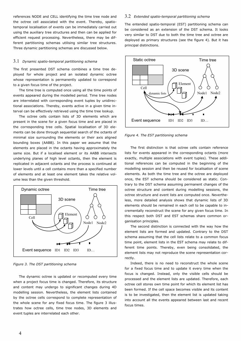
3.2 Extended spatio-temporal partitioning schema
The entended spatio-temporal (EST) partitioning schema can
be considered as an extension of the DST schema. It looks
very similar to DST due to both the time tree and octree are
deployed as primary structures (see the figure 4). But it has
principal distinctions.
Figure 4. The EST partitioning schema
The first distinction is that octree cells contain reference
lists for events appeared in the corresponding octants (more
exactly, multiple associations with event tuples). These addi-
tional references can be computed in the beginning of the
modelling session and then be reused for localisation of scene
elements. As both the time tree and the octree are deployed
once, the EST schema should be considered as static. Con-
trary to the DST schema assuming permanent changes of the
octree structure and content during modelling sessions, the
octree structure and event lists are computed once. Neverthe-
less, more detailed analysis shows that dynamic lists of 3D
elements should be remained in each cell to be capable to in-
crementally reconstruct the scene for any given focus time. In
this respect both DST and EST schemas share common or-
ganisation principles.
The second distinction is connected with the way how the
element lists are formed and updated. Contrary to the DST
schema assuming that the cell lists relate to a common focus
time point, element lists in the EST schema may relate to dif-
ferent time points. Thereby, even being consolidated, the
element lists may not reproduce the scene representation cor-
rectly.
Indeed, there is no need to reconstruct the whole scene
for a fixed focus time and to update it every time when the
focus is changed. Instead, only the visible cells should be
processed and the element lists are updated. Therefore, each
octree cell stores own time point for which its element list has
been formed. If the cell space becomes visible and its content
is to be investigated, then the element list is updated taking
into account all the events appeared between last and recent
focus times.
3D scene
Cell
Event sequence ID1 ID2 ID3 ID…
Node1 Node2
ell
Element
Time tree Dynamic octree
3D scene
Cell
Event sequence ID1 ID2 ID3 ID…
Node1 Node2
ell
Element
Time tree Static octree
dynamic lists

5
3.3 Advanced spatio-temporal partitioning schema
Finally, we present advanced spatio-temporal (AST) partition-
ing schema that can be considered as a further evolution of
the DST and EST schemas. Its main distinction is that the AST
schema first partitions the space domain by an octree and
then for each octree cell partitions the time domain by a time
tree (see the figure 5). By the construction it is very similar to
Shen‘s tree. The key difference of the proposed schema and
its principal advantage is that nodes of deployed time trees
are associated with scene events rather than scene objects.
Because of the events identify changes in the scene, the AST
partitioning schema avoids the replication of identical ele-
ments peculiar to Shen‘s tree.
As opposite to the DST and EST schemas, the AST as-
sumes that the octree is primary and time trees are secon-
dary. Therefore, only time tree nodes in the AST are associ-
ated with events. The AST schema remains lists of 3D
elements similar to the EST schema. It is deployed once in the
beginning of the modelling session, but the element lists are
formed and updated dynamically depending on parameters of
the last spatio-temporal request. It is very suitable for the re-
quests combining parameters of both time and space do-
mains, but useless for time requests because of the necessity
to lookup whole spatial structures to collect the events ap-
peared in a given time interval. This capability has been lost in
comparison with the EST schema whose time tree nodes con-
tain direct references on the associated event tuples.
Figure 5. The AST partitioning schema
4 PERFORMANCE ANALYSIS
To derive practically meaningful estimates of performance, let
a dynamic scene is represented by identical elements and by
similar appearance events so that each event adds a new
element in the scene and the final number of elements equals
to N. It is suggested that the elements are uniformly distrib-
uted over the scene space and the events are equiprobable
during the whole modelled time period.
Volume factor ν = (Δx∙Δy∙Δz)/(x∙y∙z) expresses relative
volume occupied by every element (more exactly, AABB sur-
rounding the element) with respect to overall scene dimen-
sions x, y, z. Linear factor δ = max(Δx/x, Δy/y, Δz/z) ex-
presses maximum relative size of the bounding box. Under
the additional assumption about the scene and elements pro-
portions Δx/x = Δy/y= Δz/z = δ, the volume factor takes the
value ν = δ3.
Let us define auxiliary parameters α, β, γ characterizing
the 4D modelling session. The parameter α > 0 defines rela-
tive volume density of the scene for a final time point as α = ν
N. The volume of view frustum with respect to the whole
scene space is given by the relative parameter β [0,1]. And
the relation Δt / t of the analyzed time interval Δt to whole
modelling period t is defined by the parameter γ [0,1].
All the performance estimates are derived for the average
case under the assumptions about the scene model peculiari-
ties. Let CTime is the average cost of point classification in time
tree nodes, CBox is the average cost of spatial localisation of
the given AABB in octree cells (relatively underlying subdivi-
sion planes of each higher level octant). In similar way, CCone
is the cost of testing whether the given AABB is located inside
view frustum (admitting intersections with its planes) or ex-
actly outside it. For simplicity, costs for navigating over the
trees, costs for gathering of elements and events as separate
collections are taken negligible and eliminated from the per-
formance analysis. Costs for forming and rendering of 3D
scenes are not related to the partitioning schemas and are be-
yond of the consideration too.
4.1 Deployment request Q1
First of all, let us estimate deployment costs for the presented
partitioning schemas. Costs for octree deployment can be ob-
tained independently from the time tree costs for all the
schemas. Octree deployment costs are presented only for the
EST, AST schemas. These costs are missing for the DST
schema as the octree structure and its content are perma-
nently updated during the 4D modelling session. According to
the accepted scenario, at a start time it does contain neither
elements nor cells and, therefore, does not require any com-
putations. At a finish time, it contains all the scene elements
placed in the deployed octant cells. Such costs are related to
other request types.
Under the scene model assumptions, identical elements
are localized in the leaf octants at the level L = log(1/δ) if α
1 and L(N) = 1/3 log(N) in the opposite case α < 1. Here L is
a height of the octree. The probability of simultaneous inter-
section of localized element and three underlying planes of oc-
tant of level l [1, L] equals to δl3, where δl = 2l δ is an ef-
fective relative size of the element AABB. By the octree
construction, it causes the element replication and placement
in eight children octants of the level l + 1. In similar way, the
probability of intersection of two planes and replication of the
element in four octants is equal to 3δl2 (1 – δl)
. The probabil-
ity of intersection of one plane and replication of the element
in two octants counts 3δl (1 – δl). And finally, the probability
of the element localisation exactly in one octant is (1 – δl)3.
Thereby, the average distribution of the element number
at the level l is given by the formula:
Rl = 8 δl3 + 12 δl
2 (1– δl) + 6 δl (1– δl) + (1– δl)3
Element
3D scene
Cell
Event sequence ID1 ID2 ID3 ID…
Node1 Node2
ell
Time trees
Static octree
dynamic lists

6
The average cost of element localisation in the whole oc-
tree is given by CBox R(L), where a summarizing function R(L)
is defined as Σl=1L l∙Rl. Then, the total costs for the octree de-
ployment take the value CBox R(L)N as each appearance event
requires exactly one localisation operation for the correspond-
ing element. It can be shown that the function R(L) is ex-
pressed by the formula:
R(L) = (1/98)*(5 δ323L+4 – 35 δ323L+4L – 80 δ3 – 49
δ222L+3 + 147 δ222L+3L + 392 δ2 – 147 δ2L+2 + 147 δ2L+2L +
588 δ + 49 L2 + 49 L)
with upper limit given by R(L) ≤ 4*(L+1)L.
The time trees are static structures in all the presented
schemas and the deployment costs can be directly calculated.
The binary search trees in the DST and EST schemas contain
exactly N nodes and their computing can be done in CTime
log(N!). In the AST schema time trees are formed in each of
8L leaf octants with the average number of events equal to
N/8L. Therefore, total costs to deploy all such trees within the
AST schema count CTime 8L log((N/8L)!).
By concluding, the deployment costs for DST, EST and AST
schemas are expressed by the corresponding formulae:
C1DST = CTime log(N!)
C1EST = CTime log(N!) + CBox R(L)N
C1AST = CTime 8 L log( (N/8L)! ) + CBox R(L)N
4.2 Scene reconstruction request Q2
The scene reconstruction request Q2 is executed under the
suggestion that the scene is known for the previous focus time
and it is required to update the scene for the recent focus
time. All the events appeared during this interval must be col-
lected and the corresponding updates must be done in the
scene.
The request results for the EST schema can be obtained in
two ways. Starting with the time tree, feasible events ap-
peared in the analysed time interval can be determined in CT
γN. The relative factor γ defines here the time duration over
which the scene is reconstructed. The value γ = 0 corresponds
to the confluent case when no events appear and there is no
need to update the scene. The value γ = 1 corresponds to re-
construction of the scene over the whole modelling period.
Additional checks whether the detected events appear in the
view frustum take CConeγN.
The second way assumes the primary use of the octree.
Navigation through visible octants and checks against appear-
ance of the associated events in the given time interval re-
quire CTimeβR(L)N. The factor R(L) takes into account the ex-
pected number of elements at the octree level L that differs
from the original number due to the element replication.
Applying the optimal strategy combining both methods,
the cost function takes the form:
C2EST = min( (CTime + CCone)γN, CTimeβR(L)N )
The performance estimate for the AST schema can be de-
rived in a similar way, but the lookup process should be ex-
panded on partial time trees deployed in the octree leaves.
Each such tree provides for fast binary search of those events
which appear during the given time interval in the parent oc-
tant. Gathering actual events through all visible octants and
feasible nodes, the resulting collection can be obtained and
processed to update the scene. Taking into account the uni-
form distribution of elements over the scene space and events
over the modelled time period, the expected number of events
appeared in the view frustum during the time interval is given
by the value βγR(L)N. Therefore the total costs are expressed
by the corresponding formula:
C2AST = CTime βγR(L)N
Finally, the request Q2 can be satisfied using the DST
schema. By iterating through the time tree nodes, actual
events can be identified in CTime γN. The octree is dynamically
recomputed if the focus time has been changed. For each de-
tected appearance event the associated element should be
placed into the corresponding octant according to the ac-
cepted modelling scenario. To update the octree γN elements
must be placed. As explained above, it can be done in CBox
R(L) γN. Therefore, the final performance estimate for the
DST schema takes a form:
C2DST = CTime γN + CBox R(L) γN
Here the height of the dynamic octree 1 ≤ L ≤ L depends on
the number of already placed elements as L = log(1/δ) if α γ
1, and L(N) = 1/3 log(γ N) in the opposite case α γ < 1.
4.3 Volume clipping request Q3
The volume clipping request can be executed in a way com-
mon for all the presented schemas. Again, iterating through
the octree the visible octants located in the view frustum are
determined and associated events (or elements) are collected.
Let a camera is moved so that each new view frustum takes
additional scene space volume with the relative factor β[0,1]
introduced above. To determine which octants are visible, it is
necessary to iterate approximately over β Σl=1L 8l cells from
the root down to leaves and to check whether they belong to
the view frustum or not. By expressing the sum of the geo-
metrical series the computational cost of the volume clipping
operation takes a form CCone β(8L+1-1)/7. The level parameter
corresponds to the octree height fixed for the EST and AST
schemas and varied for the DST schema depending on the
factual number of processed events and placed elements. The
determination of visible octants is a key performance issue for
the DST schema, so the following formula takes place:
C3DST = CCone β(8L+1-1)/7
The EST and AST schemas require additional updates of
the dynamic element lists. Remind that although these sche-
mas assume static deployment, the element lists have to be
modified to conform to particular time points. It avoids unnec-
essary updates of the element lists belonging to the invisible
octants and simplifies the scene reconstruction for the octants
which become visible. Therefore, to execute the volume clip-
ping request the reconstruction operation must be invocated
for those cells which become visible and whose lists do not
conform to the recent focus time. The cost estimates for the
reconstruction operation have been obtained in the previous
section. Thereby, the total costs for the volume clipping re-
quest are expressed by the following similar formulae:
C3EST = CCone β(8L+1-1)/7 + CTime βR(L)N
C3AST = CCone β(8L+1-1)/7 + CTime βγR(L)N

7
The formulae have been derived under the suggestion that the
scene reconstruction request is executed first time for the oc-
tants belonging to the changed view frustum.
4.4 Animation request Q4
The animation request assumes simultaneous changes of both
the focus time and the view camera position. Therefore it can
be represented by a pair of the scene reconstruction and vol-
ume clipping operations. As a result, its cost can be estimated
as a simple sum of the auxiliary request costs. It is true for
the DST schema:
C4DST = C2DST + C3DST
For the EST and AST schemas more adequate dependencies
can be identified as the volume clipping operations provide for
the partial scene reconstruction. Thus, the following cost rela-
tions can be established:
C4EST = C3EST
C4AST = C3AST
5 COMPARATIVE ANALYSIS
Let us compare the three presented partitioning schemas with
regards to typical requests and common performance re-
quirements imposed upon their execution. The comparative
analysis of the computational costs enables to formulate rec-
ommendations on the effective use of the schemas for large
project data. The complexity formulae obtained for all the in-
troduced requests and the specified schemas are summarised
in the table 1.
Table 1. The complexity costs for the partitioning schemas
Q1
C1DST = CTime log(N!)
C1EST = CTime log(N!) + CBox R(L)N
C1AST = CTime 8 L log((N/8L)!) + CBox R(L)N
Q2
C2DST = CTime γN + CBox R(L) γN
C2EST = min((CTime + CCone)γN, CTime βR(L)N) C2AST = CTime βγR(L)N
Q3
C3DST = CCone β(8L+1-1)/7
C3EST = CCone β(8L+1-1)/7 + CTime βR(L)N C3AST = CCone β(8L+1-1)/7 + CTime βγR(L)N
Q4
C4DST = C2DST + C3DST C4EST = C3EST
C4AST = C3AST
First of all, it can be concluded that the costs for deploy-
ment of auxiliary structures may be varied significantly. The
asymphtotic estimates of the complexity O(NlogN) coincide
each other for the time tree deployment, although the AST
schema looks more preferable for practical purposes. The oc-
tree deployment for the EST and AST schemas takes the same
costs O(Nlog2N) which are fully avoided by the DST schema.
The scene reconstruction can be efficiently done in
O(Nlog2N) for the requests assuming significant fragmentation
of time and space domains using the AST schema. Other
schemas have the same asymphtotic estimate with multipliers
larger than the factor 4/9CTimeβγ admitted by the AST
schema.
The DST schema is most efficient for the volume clipping
requests as it operates mainly with the partially deployed oc-
tree and avoids additional costs for the scene reconstruction in
latent octants. The AST looks more preferable than the EST as
it simplifies the checks for active events using multiple time
trees deployed in the octree leaves. If the time interval for the
reconstruction is relatively small for latent octants, then it
provides for performance advantage over the EST schema.
Finally, the AST and EST schemas are well suited for the
animation requests. The complexities are the same as those of
derived for the volume clipping operation. The DST schema
requires for total updates of the octree structure which are
unnecessary for other considered schemas. Each of the pre-
sented schemas has own benefits and drawbacks compared
with the other solutions. The criterion of uniformly high per-
formance for different type requests seems to be adopted for
the choice of optimal schema.
6 CONCLUSIONS
Thus, the spatio-temporal decomposition approach to 4D
modelling of large-scale industrial projects has been pre-
sented. The approach assumes special data structures and fa-
cilities to effectively execute typical requests relevant to given
time and space domains. Three partitioning schemas have
been presented and analysed to satisfy performance require-
ments. The schemas exploit coherence peculiarities of the
pseudo-dynamic, event-driven scenes appearing in 4D model-
ling and planning applications. The derived theoretical esti-
mates of the complexity as well as the conducted computa-
tional experiments prove benefits of the schemas and their
wide potential use.
REFERENCES
Finkelstein, A., Jacobs, C.E. & Salesin, D.H. 1996. Multiresolu-
tion video. In Proceedings of ACM SIGGRAPH ’96: 281–
290.
GSA BIM 2009. U.S. General Services Administration, Public
Buildings Service, Technical Report ―GSA Building Informa-
tion Modeling Guide Series 04 – 4D Phasing‖, 2009,
http://www.gsa.gov/bim/.
Heesom, D. & Mahdjoubi, L. 2004. Trends of 4D CAD applica-
tions for construction planning. Construction Management
and Economics, 22: 171–182.
Jimenez, P., Thomas, F. & Torras C. 2001. 3d collision detec-
tion: a survey. Computers and Graphics, 25: 269–285.
Klosowski, J.T., Held, M., Mitchell, J.S.B., Sowizral, H. & Zikan,
K. 1998. Efficient collision detection using bounding vol-
ume hierarchies of k-DOPs. Visualization and Computer
Graphics, IEEE Transactions on Volume 4, Issue 1: 21 –
36.
Retik, A. 1993. Visualization for decision making in construc-
tion planning. Visualization and intelligent design in engi-
neering and architecture, J.J. Connor, et al., eds., Elsevier
Science(New York, NY): 587-599.
Seliga, C. 2007. Revel Selects Synchro for $2 Billion Atlantic
City Casino Project. Prime Newswire June-2007, Coventry,
England.
Shagam, J. & Pfeiffer, J. 2003. Dynamic Irregular Octrees.
Technical Report NMSU-CS-2003-004.
Shen, H.W., Chiang, L.J. & Ma, K.L. 1999. A fast volume ren-
dering algorithm for time-varying field using a time-space

8
partitioning (TSP) tree. In Proc. IEEE Visualization: 371–
377.
Sriprasert, E. & Dawood, N. 2002. Requirements identification
for 4D constraint-based construction planning and control
system. Conference Proceedings – Distributing Knowledge
in Building, University of Teeside, Middlesbrough.
Sudarsky, O. & Gotsman, C. 1999. Dynamic Scene Occlusion
Culling. In Hans Hagen, editor, IEEE Transactions on Visu-
alization and Computer Graphics, volume 5 (1): 13–29.
IEEE Computer Society.
Whang, J.W., Song, J.W., Chang, J.Y., Kim, J.Y., Cho, W.S.,
Park, C.M. & Song I.Y. 1995. Octree-R: An adaptive octree
for efficient ray tracing. IEEE Transactions on Visualization
and Computer Graphics, 1(4): 343–349.
Zhiyan D.Y.J. & Chiang H.W.S. 2009. Out-of-core volume ren-
dering for time-varying fields using a space-partitioning
time (SPT) tree. Visualization Symposium, PacificVis '09:
73 – 80.