5 identification using prediction error methods - svibs.com · 5 identification using prediction...

y( tk ) � H(q ,� )e( tk ) , k � 1, 2, ... , N

E e( tk )e T( tk�s ) � �(� )�(s )

m�na �p

Identification using Prediction Error Methods 87

(5.1)

5 Identification using Prediction ErrorMethods

The previous chapters have shown how the dynamic behaviour of a civil engineeringstructure can be modelled by a discrete-time ARMAV model or an equivalentstochastic state space realization. The purpose of this chapter is to investigate howan estimate of a p-variate discrete-time model can be obtained from measurementsof the response y(t ). It is assumed that y(t ) is a realization of a Gaussian stochastick k

process and thus assumed stationary. The stationarity assumption implies that thebehaviour of the underlying system can be represented by a time-invariant model. Inthe following, the general ARMAV(na,nc), for na � nc, model will be addressed. Inchapter 2, it was shown that this model can be equivalently represented by an m-dimensional state space realization of the innovation form, with . No matterhow the discrete-time model is represented, all adjustable parameters of the modelare assembled in a parameter vector �, implying that the transfer function descriptionof the discrete-time model becomes

The dimension of the vectors y(t ) and e(t ) are p × 1. Since there is no unique wayk k

of computing an estimate of (5.1), it is necessary to select an appropriate approachthat balances between the required accuracy and computational effort. The approachused in this thesis is known as the Prediction Error Method (PEM), see Ljung [71].The reason for this choice is that the PEM for Gaussian distributed prediction errorsis asymptotic unbiased and efficient. Further, the use of the PEM enables an estimateof the associated uncertainties of the estimated model parameters. The precision ofthe PEM does not come for free. It is as such not the most computationally fastapproach compared to other estimation techniques. However, in applications such asVBI computational time is not the issue compared to estimation accuracy. In suchcases, one would probably rather wait for an accurate estimate instead of using a lessaccurate but computationally fast approach. The PEM algorithm used in this thesisis of the off-line type, which implies that it uses all available data to update theestimates of the model parameters. This is in contrast to the so-called on-line orrecursive algorithms that update the estimated model parameters from sample pointto sample point. The choice of the off-line algorithm is reasonable, since themeasured data are assumed stationary within a given time series, and since theapplied models are time-invariant. At the same time, this algorithm does not sufferthe difficulties experienced with the use of the on-line algorithm, with regard to e.g.initialization. A description of the on-line PEM algorithms can be found in Goodwinet al. [31], Ljung [71], Norton [82] and Söderström et al. [105]. Applications on theuse of recursive ARMA and ARMAV models for on-line identification of time-varying system can be found in Kirkegaard et al. [55], [56] and [60].

�( tk ,� ) � y( tk ) � y( tk | tk1 ;� )

y( tk | tk1 ;� ) � L(q ,� )y( tk )

y( tk ) � �A1 y( tk1 ) � ... � A na y( tkna ) �

e( tk ) � C1 e( tk1 ) � ... � C nc e( tknc )

E e( tk )eT( tk�s ) � �(� )�(s )

x( tk�1 | tk ;� ) � A(� ) x( tk | tk1 ;� ) � K(� )e( tk )

y( tk ) � C(� ) x( tk | tk1 ;� ) � e( tk )

E e( tk )eT( tk�s ) � �(� )�(s )

H(q ,� ) � A1(q ,� )C(q ,� )

A(q ,� ) � I � A1 q 1� ... � A na q na

C(q ,� ) � I � C1 q 1� ... � C nc q nc

y( tk | tk1 ;� )

y( tk | tk1 ;� )

88 Identification using Prediction Error Methods

(5.2)

(5.3)

(5.4)

(5.5)

(5.6)

All systems are in principle stochastic, which means that the output y(t ) at the timek

k cannot be determined exactly from data available at the time k-1. It is thus valuableto know at the time k-1 what the output y(t ) of the stochastic process is likely to bek

at time k.

Therefore, it makes sense to determine the model parameter vector � so that theprediction error, defined as

is as small as possible. is the predicted response at the time k based onthe parameters �, and given available data up to and including the time k-1, i.e.

where L(q,�) is a p-variate prediction filter having a pure time delay between y(t )k

and . This filter can be constructed in a number of ways, but it willalways be based on the model parameters �. Once the model structure and this filterhave been chosen, the prediction errors are calculated from (5.2). In this thesis,system identification of a p-variate stochastically excited linear and time-invariantsystem is either performed using the p-variate ARMAV(na,nc) model, defined intheorem 2.3 as

or by using the innovation state space system

The transfer function of the ARMAV(na,nc) model is defined as

and the transfer function of the innovation state space system is defined as

H(q ,� ) � C(� ) Iq � A(� ) 1K(� ) � I

L(q ,� ) � I � H1(q ,� )

y( tk ) � H(q ,� )e( tk ) � H(q ,� ) � I e( tk ) � e( tk )

e(tk) y(tk)


(5.7)

(5.8)

(5.9)

Having chosen the model structure, it is necessary to make the following choices todefine a prediction error method for minimization of �(t ,�).k

� Choice of prediction filter L(q,�).� Choice of a scalar-valued function that can assess the performance of the

predictor.� Choice of procedure for minimization of this performance function.

The first three sections of this chapter describe how to make the three choices listedabove. Section 5.4 concerns, organization of the parameters of the chosen modelstructure in the parameter vector �, and describes how the gradient of the chosenprediction filter is calculated. In section 5.5, the statistical properties of the predictionerror method are analysed. These properties are statistical asymptotic efficiency andconsistency of the PEM estimate, and asymptotic distribution of the estimatedparameters. Section 5.6 deals with the problems of obtaining reliable initial estimatesof the model parameters used in the PEM. Finally, in section 5.7, guidelines forvalidation of an identified model and model order selection will be provided.

5.1 Choice of Prediction Filter

In this section it is shown how the prediction filter may appear when the modelstructure is the ARMAV model or the innovation state space system. If the modelstructure is the p-variate ARMAV(na,nc) model shown in (5.4) then the predictionfilter may appear as in the following theorem.

Theorem 5.1 - The Prediction Filter of the ARMAV Model

If the ARMAV model is represented by a transfer function description as in (5.6) then theprediction filter L(q,��) in (5.3) is given by

The filter will only be asymptotically stable if all eigenvalues of H (q,��) are inside the-1

complex unit circle, see Söderström et al. [105].

Proof:

From (5.1), it is seen that

By assuming that H(q,��) is invertible the knowledge of the response y(t ), for s � k-1 impliess

the knowledge e(t ) for s � k-1. In other words, can be replaced by using (5.1). Thes

y( tk | tk1 ;� ) � H(q ,� ) � I e( tk )

� H(q ,� ) � I H1(q ,� )y( tk )

� I � H1(q ,� ) y( tk )

� L(q ,� )y( tk )

�( tk ,� ) � y( tk ) � y( tk | tk1 ;� )

� y( tk ) � I � H1(q ,� ) y( tk )

� H1(q ,� )y( tk )

y( tk | tk1 ;� ) � y( tk ) � �( tk ,� )

� �A1(� )y( tk1 ) � ... � A na(� )y( tkna ) �

C1(� )�( tk1 ,� ) � ... � C nc(� )�( tknc ,� )

x( tk�1 | tk ;� ) � A(� ) � K(� )C(� ) x( tk | tk1 ;� ) � K(� )y( tk )

y( tk | tk1 ;� ) � C(� ) x( tk | tk1 ;� )

e(tk)

H1(q,�) � C1(q,�)A(q,�)

90 Choice of Prediction Filter

(5.10)

(5.11)

(5.12)

(5.13)

first term of (5.9) is therefore known at the time t . Since the has zero mean thek-1

conditional expectation of (5.9) with respect to y(t ), for s � k-1, is given bys

which proves the theorem. a

If the prediction filter (5.8) is combined with (5.2) the predictor of the model appearsas

Combining this result with the fact that for theARMAV(na,nc) model yields

This relation reveals that the predictor of the ARMAV model is nonlinear, since theprediction errors themselves depend on the parameter vector �. This indicates that aniterative minimization procedure has to be applied.

Now let (5.1) be represented by the innovation state space system (5.5). Theprediction filter may for this representation of (5.1) be given by the followingtheorem.

Theorem 5.2 - The Prediction Filter of the Innovation State Space System

The predictor of the innovation state space system (5.5) is given by

L(q ,� ) � C(� ) Iq � A(� ) � K(� )C(� ) 1K(� )

x( tk�1 | tk ;� ) � A(� ) x( tk | tk1 ;� ) �

K(� ) y( tk ) � C(� ) x( tk | tk1 ;� )

y( tk | tk1 ;� ) � C(� ) x( tk | tk1 ;� )

QN (� ) �1N�

N

k1� ( tk ,� )�T( tk ,� )

y( tk | tk1 ;��)

�(tk,�)

�(tk,�)

�(tk,�)

QN(�)


(5.14)

(5.15)

(5.16)

Since the input in (5.13) is y(t ), and the output is , the system is an internalk

description of L(q,��). By introduction of the shift operator q the prediction filter can formallybe represented by

This filter will only be asymptotically stable if the eigenvalues of the matrix A(��)-K(��)C(��)lie inside the complex unit circle, see Söderström et al. [105].

Proof:

The innovation state space representation in (5.5) is derived from the steady-state Kalmanfilter, see theorem 2.2,

which by rearrangement of the state equation looks as (5.13). a

In both cases the predictors are mean square optimal if the prediction errors areGaussian distributed, see e.g. Goodwin et al. [31], Ljung [71] and Söderström et al.[105]. It should be pointed out that is assumed to be Gaussian white noise inthe above derivations. However, it is possible to compute and apply L(q,�) even ifthe Gaussian assumption is not satisfied by the data. However, if is no longerGaussian white noise, then the prediction filter is no longer optimal. In any case,given a model structure and its parameters in a vector �, it is now possible toconstruct a prediction filter L(q,�). Based on this filter and available data y(t ) thek

prediction errors can now be computed. The next step in the derivation of aPEM algorithm is the definition of a criterion function.

5.2 Choice of Criterion Function

The criterion function has to be a scalar-valued function of all prediction errors�(t ,�), k = 1 to N. The purpose of this function is to assess the performance of thek

predictor. If the prediction errors �(t ,�) are assumed to be Gaussian distributed, ank

optimal set of parameters � must minimize the covariance matrix of �(t ,�). It isk

therefore reasonable to base the minimization of the prediction errors on thefollowing function , see Söderström et al. [105]

h(QN (� ) ) � det QN (� )

�N � arg min�

det1N�

N

k1� ( tk ,� )�T( tk ,� )

� arg min�

VN (� )

�i�1N � �

iN � µ i V

1N (�i

N) �V TN (�i

N)

µ i � arg minµ

V �iN � µ V 1

N (�iN) �VN (�i

N)

QN(�)

QN(�) QN(�)

�N

�iN

�i�1N

�VN (� ) VN (� )µ i

92 Choice of Minimization Procedure

(5.17)

(5.18)

(5.19)

(5.20)

However, it is only possible to use directly as a criterion function, when theprediction errors constitute a scalar sequence. In the general case, a monotonicallyincreasing function h( ) that maps as a scalar value must be chosen. Achoice of a monotonically increasing function is

This function is preferred, because it corresponds to the criterion function of themaximum likelihood method for Gaussian distributed prediction errors, see Akaike[2], Box et al. [16] and Ljung [71]. The off-line parameters estimate, based on Nsamples, and returned in is therefore obtained as the global minimum point of thecriterion function (5.17), i.e.

In (5.18) arg min should be read as the argument that minimizes the criterionfunction. Notice that the criterion function for short is denoted V (�). The criterionN

function is sometimes referred to as the loss function, since it is a measure of the lossof information contained in the data.

5.3 Choice of Minimization Procedure

The question now is how to satisfy (5.18), i.e. how to minimize the loss functionV (�). As shown in section 5.1, the prediction filter as well as the prediction errorsN

depend on currently estimated parameters, implying that the search for a minimumbecomes nonlinear. The applied search-scheme is of the full-Newton or Newton-Raphson type, see e.g. Ljung [71], Söderström et al. [105] and Vanderplaats [108].It updates the estimate of n × 1 parameter vector of the ith iteration to a newestimate using the following update procedure

where is the 1 × n gradient vector and the n × n Hessian matrix of thecriterion function V (�). In strict theoretical sense the coefficient is equal to 1.N

However, in practice the step size is often too long and needs adjustment. Thereforeµ should be chosen as the argument that minimizes the following relation,i

Söderström et al. [105]

�VN (� ) � �2VN (� ) 1N�

N

k1�T( tk ,� )Q1

N (� )�T( tk ,� )

�( tk ,� ) �

� y( tk | tk1 ;� )

��

�VN (� )

�QN (� )� VN (� )Q1

N (� )

VN (� ) � 2VN (� ) 1N�

N

k1�( tk ,� )Q1

N (� )�T( tk ,� )

y( tk | tk1 ;� )

VN (� )

VN (� )


(5.21)

(5.22)

(5.23)

(5.24)

Besides the use for adjustment of the step size, µ can also be used to ensure that thei

eigenvalues of the prediction filter stay inside the complex unit circle. Thecomputational burden of the search procedure is the calculation of the gradient andof the Hessian matrix of the criterion function, and the only algebraic differencebetween the estimation of the ARMAV model and the corresponding state spacerepresentation is the calculation of the gradient of the predictor.

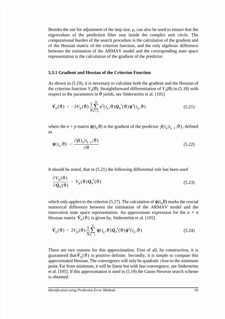
5.3.1 Gradient and Hessian of the Criterion Function

As shown in (5.19), it is necessary to calculate both the gradient and the Hessian ofthe criterion function V (�). Straightforward differentiation of V (�) in (5.18) withN N

respect to the parameters in � yields, see Söderström et al. [105]

where the n × p matrix �(t ,�) is the gradient of the predictor , definedk

as

It should be noted, that in (5.21) the following differential rule has been used

which only applies to the criterion (5.17). The calculation of �(t ,�) marks the crucialk

numerical difference between the estimation of the ARMAV model and theinnovation state space representation. An approximate expression for the n × nHessian matrix is given by, Söderström et al. [105]

There are two reasons for this approximation. First of all, by construction, it isguaranteed that is positive definite. Secondly, it is simple to compute thisapproximated Hessian. The convergence will only be quadratic close to the minimumpoint. Far from minimum, it will be linear but with fast convergence, see Söderströmet al. [105]. If this approximation is used in (5.19) the Gauss-Newton search schemeis obtained.

�i�1N � �

iN � µ i R

1N ( �i

N )FN( �iN )

RN(� ) � �N

k1�( tk ,� )Q1

N (� )�T( tk ,� )

FN(� ) � �N

k1�( tk ,� )Q1

N (� )�( tk ,� )

y( tk | tk1 ;� ) � L(q ,� )y( tk )

�Ti ( tk ,� ) �

�L(q ,� )��i

y( tk ) , i�1, 2, ... , n

y( tk | tk1 ;� )y( tk | tk1 ;� )

94 Calculating the Predictor Gradient

(5.25)

(5.26)

(5.27)

(5.28)

Definition 5.1 - The Gauss-Newton Search Scheme

If the gradient (5.21) of the criterion function is inserted into (5.19), together with theapproximated Hessian in (5.24), the Gauss-Newton search-scheme

is obtained. The n × n matrix R (��) and the n × 1 vector F (��) given byN N

and µ chosen according to (5.20). ai

Because the approximated Hessian is guaranteed positive definite, the criterionfunction will decrease in every iteration by proper choice of µ . However, if the modeli

is overparameterized, i.e. has too many parameters compared to what is actuallyneeded, the approximated Hessian might be close to singular and therefore difficultto invert. Various techniques have been proposed in order to overcome this problem.A well-known technique is the Marquardt-Levenberg search scheme, Levenberg [70]and Marquardt [74]. However, if a good initial estimate of � is available, it is theexperience that the Gauss-Newton search-scheme works very well for properlyselected model structures. This search scheme is standard in the System Identifica-tion toolbox for use with MATLAB, see Ljung [72], and has been used in severalidentification application, see e.g. Andersen et al. [6], Asmussen et al. [9], Brinckeret al. [17], Kirkegaard et al. [56] and [57].

5.4 Calculating the Predictor Gradient

As stated previously, the only significant difference between estimation of theARMAV model and the innovation state space representation is the way the predictor

and its gradient �(t ,�) are calculated. In (5.3), it was shown thatk

could be obtained by filtering the data through a prediction filter as

implying that the n rows of �(t ,�) are obtained fromk

� � col A1 . . A na , C1 . . C nc

C(q ,� ) y( tk | tk1 ;� ) � C(q ,� ) � A(q ,� ) y( tk )

�Ti ( tk ,� ) � �C 1(q ,� )Qr,c y( tkd )

i�1, ... , na�p 2

d � int ��

i

p 2� 1

c � int ��

1 � d � 1 p 2

p� 1

r � 1 � d � 1 p 2� c � 1 p


(5.29)

(5.30)

(5.31)

However, before the gradient can be calculated, it is necessary to determine how theparameters of the model structures are organized in the parameter vector �.

5.4.1 The Predictor Gradient of the ARMAV Model

The p-variate ARMAV(na,nc) model was defined in (5.4). For simplicity, it isassumed that all parameters of the p × p coefficient matrices A and C are adjustable.i i

The n × 1 parameter vector � is organised in the following way

where col means stacking of all columns of the argument matrix. The total numberof adjustable parameters in � is as such n = (na+nc)p . 2

Denote the (i,j)th element of the kth auto-regressive coefficient matrix A by a . Thisk i,j,k

element is recovered as element number (k-1)p +(j-1)p+i of �. In a similar manner,2

the (i,j)th element of the kth moving average coefficient matrix C , denoted c , cank i,j,k

be recovered as element number (na+k-1)p +(j-1)p+i of �.2

The predictor of the ARMAV model is given by (5.27), with the prediction filterdefined in (5.8). If the definition H(q,�) = A (q,�)C(q,�) is inserted, the predictor-1

can be formulated as

Introduce a p × p matrix Q whose elements are all zero except the element (j,k) thatj,k

is equal to 1. Further, define int |x| as an operator that returns the integral part of theargument x. The ith row of �(t ,�) can then be found by partial differentiation ofk

(5.30) with respect to � . If � is one of the auto-regressive parameters then � (t ,�)i i i k

is given by

�Ti ( tk ,� ) � C 1(q ,� )Qr,c �( tkd ,� )

i�na�p 2�1, ... , na�nc p 2

d � int ��

i

p 2� na � 1

c � int ��

1 � na � d � 1 p 2

p� 1

r � 1 � na � d � 1 p 2� c � 1 p

A(� ) �

0 I . . 0 0

0 0 . . 0 0

. . . . . .

. . . . . .

0 0 . . 0 I

�A na �Ana1 . . �A2 �A1

, K(� ) �

h(1)

h(2)

.

.

h(na�1)

h(na )

C(� ) � C � I 0 . . 0 0

�Ti ( tk ,� ) �

T

i�p 2 ( tk1 ,� )�i�p 2 ( tk1 ,� )

96 Calculating the Predictor Gradient

(5.32)

(5.33)

(5.34)

However, if � is one of the moving average parameters then � (t ,�) is given byi i k

In both cases, it is seen that � (t ,�) is obtained as the output of a multivariate filter.i k

The computation can as such be done in a fast and efficient manner. It should also benoted that simply is , i.e. � (t ,�) is obtained directly fromi k

without any computation. This means that each of the filters (5.31) and(5.32) only needs to be applied p times, i.e. exactly the number of times that2

correspond to the number of elements of Q .j,k

5.4.2 The Predictor Gradient of the State Space System

If the model structure is of the innovation state space form, it is necessary to decideon the realization for use. For illustrative purposes the observability canonical statespace realization of the p-variate ARMAV(na,nc), with na � nc, will be used, seetheorem 2.5. For this particular realization of the innovation state space system (5.5),the matrices A(�) and K(�) which contain all the adjustable parameters, are given by

The matrix C(�) only contains trivial parameters as

� �

col �A

col �K

�A� �A na �Ana1 . . �A2 �A1 , �K

�

h(1)

h(2)

.

.

h(na�1)

h(na )

�i ( tk�1 ,� ) � A(� )�K(� )C �i ( tk ,� ) � QAr,c x( tk | tk1 ;� )

�Ti ( tk ,� ) � C�i ( tk ,� )

i�1, ... , na�p 2

c � int �� i�1

p� 1

r � na�c p � i

na �p × na �pna �p × p

n�2na �p 2

x( tk | tk1 ;� ) �i(tk | tk1 ;�)na �p × na �p

QAr,c

na �p × p QKr,c


(5.35)

(5.36)

(5.37)

The dimension of A(�) is . All non-trivial and adjustable parametersof this matrix are located in the last p rows. The dimension of K(�) is andall parameters of this matrix are adjustable. The total number of adjustableparameters of this realization is as such . These are assembled in the n ×1 parameter vector � as

where

It should be noted, that the first half of the parameters of � only relates to A(�),whereas the second half only relates to K(�). Having estimated � the correspondingARMAV model can be determined by use of theorem 2.3.

Denote the partial derivative of with respect to � by .i

Consider the parameters of the first half of �. Introduce the matrixwhose elements are all zero except element (r,c) which is equal to 1. The gradient

� (t ,�), defined in (5.28), is then obtained by differentiation of (5.13) with respecti k

to � asi

Now consider the parameters of the second half of �. Introduce the matrix whose elements are all zero except element (r,c) which is equal to 1. The gradient� (t ,�) is then given byi k

�i ( tk�1 ,� ) � A(� )�K(� )C �i ( tk ,� )�QKr,c �( tk ,� )

�Ti ( tk ,� ) � C�i ( tk ,� )

i�na�p 2�1, ... ,2na�p 2

c � int ��

i�na�p 2�1

na�p� 1

r � 1�c�p na�p � i

y( tk ) � H0(q )e0( tk ) , E e0( tk )eT0 ( tk�s ) � �0�(s )

DT (S ,M ) � � | H0(q ) � H(q ,� ) , �0 � �(� )

DT (S,M)

S�M(�).DT (S,M)

S�M(�0). DT (S,M)S�M(�).

98 Properties of the Prediction Error Method

(5.38)

(5.39)

(5.40)

Each of the state space systems (5.37) and (5.38) has to be applied na�p times in2

order to construct �(t ,�). By now it is possible to construct a complete PEMk

algorithm that implements the Gauss-Newton search-scheme. However, to appreciatethe PEM approach fully some of the statistical properties associated with it will beconsidered in the following section. The actual implementation is discussed inchapter 7. The PEM approach using the Gauss-Newton search scheme is alsoimplemented in Ljung [71], for several different model structures, including theARMA model.

5.5 Properties of the Prediction Error Method

In this section, it will be shown that under a certain assumption the estimatedparameters possess some appealing statistical properties. As an introduction to thesetopics the uniqueness of an estimated ARMAV model will be considered.

5.5.1 Uniqueness of the Model Structure Parametrization

Define the true linear and discrete-time system S as

Introduce the set as

and let it consist of those parameter vectors � for which a chosen model structure Mgives a perfect description of the system, i.e. The set might be empty orconsist of several points. However, in the following it will be assumed that only includes one parameter vector � , that satisfies If consists0

of several points, it implies that several models satisfy This situation is

A(q ,� )y( tk ) � C(q ,� )e( tk ) , E e( tk )eT( tk�s ) � �(� )�(s )

A0(q )y( tk ) � C0(q )e0( tk ) , E e0( tk )eT0( tk�s ) � �0�(s )

A0(q ) � I � A0,1 q 1� ... � A0,na0

qna0

C0(q ) � I � C0,1 q 1� ... � C0,nc0

qnc0

A10 (q )C0(q ) � A1(q ,� )C(q ,� ) , �0�(s ) � �(� )�(s )

Q�

(� ) � limN��

QN (� ) � E �( tk ,� )�T( tk ,� )

V�

(� ) � det Q�

(� ) � det E � ( tk ,� )�T( tk ,� )

DT (S,M)

QN(�)

�N��

��


(5.41)

(5.42)

(5.43)

(5.44)

(5.45)

encountered in cases where model structures are overparameterized, see Ljung [71]and Söderström et al. [105]. The question is when a model structure is over-parameterized. To answer this, consider the ARMAV model defined in (5.4)

and let the true system be given by

The identities in (5.40) that define the set then become

It is assumed that A (q) and C (q) are left coprime, i.e. their greatest common divisor0 0

is an unimodal matrix, implying that na � nc . For (5.43) to have a solution, it is0 0

necessary that na� na and nc� nc , and A(q,�) and C(q,�) must be left coprime, see 0 0

e.g. Gevers et al. [29] and Kailath [48]. In other words, the degree of A(q,�) must atleast be equal to the degree of A (q), and similar, the degree of C(q,�) must at least0

be equal to the degree of C (q). If both na = na and nc = nc are fulfilled, the0 0 0

solution will be unique, which implies that only one parameter vector � will exist.0

5.5.2 Convergence and Consistency of the Estimate

It is interesting to analyse what happens when the number of samples N tends toinfinity. Since y(t ) is assumed stationary and ergodic the sampled covariance matrixk

of the prediction errors converges to the corresponding expected values

implying that

If the convergence is uniform, see Ljung [71], it follows that the parameters converge to a minimum point of V (�), described by the vector , with the

�

probability 1 as N tends to infinity. If coincides with the true parameters � the0

�� 0 � �

�

P( �N ) � F1

F � E� lnp(Y N ,�0 )

��0

T� lnp(Y N ,�0 )

��0

�N ��

�N

�N �N

�N

�N

100 Properties of the Prediction Error Method

(5.46)

(5.47)

(5.48)

PEM estimate is said to be consistent, in which case Q (�) = � . If , on the� 0

other hand, does not coincide with � the estimate will be biased, i.e. non-consistent.0

The bias � is then given by��

The PEM estimate will be consistent if the true system S is contained in the modelstructure M, and if �(t ,�) is a white noise. k

5.5.3 Asymptotic Distribution of the Estimated Parameters

Besides establishing that the PEM estimate converges, it might be desirable tomeasure its performance against some standard. A standard for estimating covarianceis provided by the Cramer-Rao bound, see e.g. Söderström et al. [105]. The boundapplies to any unbiased estimate of the true parameters � using available data0

y(t ). Since noise most certainly is present, at least some of the data are stochastick

variables, described by their joint probability density function p(Y ,� ), with YN N0

defined as Y = {y(t ), y(t ), ... , y(t )} . As seen p(Y ,� ) is influenced by the trueN T NN N-1 0 0

parameters � . The covariance P( ) of cannot be less that the Cramer-Rao lower0

bound F -1

where

is the Fisher information matrix, see e.g. Söderström et al. [105]. Without attemptinga detailed interpretation of F, this matrix associates the lowest potential covarianceF of an estimate with the most information about it. If the covariance of in-1

(5.47) equals F then the estimator is said to be statistically efficient. This implies-1

that no other unbiased estimate will have lower covariance. The PEM estimate willbe statistically efficient if, see Ljung [71] and Söderström et al. [105]:

� The true system S is contained in the model structure M� �(t ,�) is a white noise. k

� The chosen criterion function is (5.17).

On the basis of these assumptions an estimate of the covariance associated with is given by, see Söderström et al. [105]

P( �N ) � �N

k1�( tk , �N )Q1

N ( �N )�T( tk , �N )1

� R1N ( �N )

x( tk�1 ) � A(� )x( tk ) � w( tk )

y( tk ) � C(� )x( tk ) � v( tk )

K(� ) � M � A(� )� CT(� ) � � C(� )� CT(� )1

� � A(� )�AT(� ) �

M� A(� )�CT(� ) �� C(� )�CT(� )1

M� A(� )�CT(� )T

A(� ) C(� ) ��E [y(tk)yT(tk) ]M�E [x(tk�1)yT(tk) ]


(5.49)

(5.50)

(5.51)

(5.52)

where R (�) is obtained from (5.26).N

5.6 Constructing Initial Parameter Estimates

The Gauss-Newton search scheme given in definition 5.1 is started by supplyinginitial parameter estimates. Even though the convergence rate is fast, it is vital thatthe initial parameter estimates are accurate to avoid unnecessary iterations. Thissection investigates how such initial estimates can be obtained in a fast manner.

5.6.1 Stochastic State Space Realization Estimation

Assume that initial parameter estimates of the system matrices {A(�), K(�), C(�)}ofthe innovation state space system given in section 2.2.3 are desired. Such estimatescan be obtained from several different algorithms, known as stochastic state spaceestimators. Consider the stochastic state space system

Given the dimensions of the system and measured system response y(t ), for k = 1 tok

N, the common output from these algorithms are estimates of the system matrices,denoted and , and the covariance matrices and

. The Kalman gain matrix can then be estimated as

by the solution of the algebraic Riccati equation

The estimated realizations are typically balanced, see section 7.1. However, if theestimated realization is observable, it can be transformed to e.g. the observabilitycanonical form by the similarity transformation of definition 2.2. If the statedimension divided by the number of output equals an integral value n, the realizationcan also be converted to an ARMAV(n,n) model, see theorem 2.3.

A0(q )y( tk ) � C0(q )e( tk )

AH(q )y( tk ) � e( tk )

A(q ,� )y( tk ) � C(q ,� ) � I e( tk ) � e( tk )

�( tk ,� ) � y( tk ) � A1(q ,� ) C(q ,� ) � I e( tk )

e( tk )

e( tk )

102 Constructing Initial Parameter Estimates

(5.53)

(5.54)

(5.55)

(5.56)

The stochastic state space realization estimators can as such be powerful tools forinitialization of the PEM algorithm both for the innovation state space representationand the ARMAV(n,n) model. These estimators can be divided into covariance anddata driven algorithms. The parameter estimates of the covariance driven algorithmsare obtained by a decomposition of Hankel matrices that consist of sampled laggedcovariances �(i) of the measured response y(t ). Such algorithms have been studiedk

by e.g. Aoki [11] and Hoen [38] and are known as e.g. the Matrix Block Hankelestimator. The data driven algorithms are of more recent origin. In these algorithmsthe system matrices are estimated by a decomposition of Hankel matrices thatconsists of the measured data. This is a more powerful estimation approach, since theestimation of the covariance matrices of the measurements are eliminated. Thesealgorithms have been studied extensively in De Moor et al. [20], Kirkegaard et al.[54] and Van Overschee et al. [107]. Common to the estimators is that they rely onthe numerical reliable Singular Value Decomposition (SVD). The performance ofboth covariance and data-driven stochastic state space estimator for identification ofcivil engineering structures is studied in e.g. Andersen et al. [6], Hoen [38] andKirkegaard et al. [54].

5.6.2 Multi-Stage Least-Squares Estimation

This section describes a least squares approach for estimation of an ARMAV(na,nc)model of arbitrary orders na and nc. In the following it is assume that the true systemis described by an ARMAV model

Since this model can be approximated arbitrarily well by a high-order ARV model

as the number of samples N tends to infinity, an estimated ARMAV model isobtained from, see Hannan et al. [34], Ljung [71] and Mayne et al. [75]

Since can be determined before hand from (5.54) by simple linear least squaresestimation of A (q), the model (5.55) is a multivariate ARX model. Such a model canH

also be solved by a linear least squares technique and estimates of A(q,�) and C(q,�)can be extracted. This approach can be refined iteratively by repeating the estimationof the ARX model with an updated external input . The prediction error �(t ,�)k

of (5.55) is obtained from

e( tk ) � �( tk ,� )

e( tk )


(5.57)

and the updated external input is then given by

This approach is a fast and reliable way of obtaining initial parameter estimates, sinceonly linear least-squares estimation is involved. The estimates of the parameters ofmodels of moderate size typically converges after 20-40 iterations. However, asstated in Piombo et al. [93], the number of iterations is strongly dependent upon thechoice of sampling interval.

5.7 Model Structure Selection and Model Validation

In system identification both the determination of an appropriate model structureM(�) and model validation are important for obtaining a successful model of the truesystem S, see section 5.5.1. In that section, it was shown that the model structuremust be large enough to contain the true system. However, overparameterization ofa model structure should be avoided since this leads to unnecessary complicatedcomputations in the estimation process, and increases the uncertainty on thesignificant parameters of the model. Underparameterization of a model structureshould also be avoided, since this means that the true system cannot be fullydescribed by the model. This inadequacy of the model might as such lead to aninaccurate description of the system. The purpose of this section is to quote somebasic methods that can be used to obtain an appropriate model structure and tovalidate the best model pointed out within the chosen structure. To obtain anappropriate and adequate model structure three choices have to be made in a sensibleway. These choice are:

� Choice of number of sensors to use.� Choice of an adequate model structure.� Choice of the dimension of the model.

The next three sections concern these choices, whereas the fourth section concernsthe model validation of the chosen model structures.

5.7.1 Choice of Number of Sensors to Use

The number of sensors to use is usually decided prior to the system identificationsession. The sensors might e.g. be a build-in part of the structure. In addition, it alsodepends on the actual application; if mode shapes are desired for some reason it isnecessary to use several sensors and to place them on locations that can provide anoptimal description of the mode shapes. There might be several reasons for usingseveral sensors. Since the number of independent model parameters of e.g. theARMAV model depends on the square of the number of sensors, it is desirable tolimit the number of sensors as a consequence of the parsimony principle. This

E WN( �N ) � � 1 �mN

WN( �N ) � E �2( tk , �N )

�N

�N�N

�N

�N

�Nm

N

m� (20�19) �12�39

104 Model Structure Selection and Model Validation

(5.58)

(5.59)

principle states that out of two or more competing models which all explain the datawell, the model with the smallest number of independent parameters should bechosen, see also Söderström et al. [105].

The effect of the parsimony principle can be illustrated for a univariate ARMA modelby letting N tend to infinity and assume the that true system belongs to the selectedclass of models. An expression for the expected prediction error variance, where theexpectation is with respect to is given by, see e.g. Söderström et al. [105]

m is the dimension of the parameter vector and W ( ) is a scalar assessmentN

measure that must be a smooth function and be minimized when = � . In the0

scalar case W ( ) equalsN

which is the prediction error variance when the corresponding model to � is used.0

It is seen that this measure of accuracy only depends on the number of data N and thenumber of adjustable or free parameters in the model m. The model structure M(�)and the experimental conditions do not affect the result contrary to the asymptoticexpression for the estimated covariance of the estimate given in (5.49) in section5.5.3. In other words, it is in some cases more relevant to consider (5.58) instead of(5.49) for the accuracy of a system identification problem. Further, (5.58) states thatthe expected prediction error variance E[W ( )] increases with a relative amountN

. Thus, there is a penalty using models with an unnecessarily high number ofparameters. This is in conflict with the fact that flexible models are needed to ensuresmall bias. So clearly a compromise has to be found. Increasing the number ofparameters will reduce the bias and increase the variance. The question how to reacha sensible compromise is the key point of the system identification process. Thus, theprimary issue of the parsimony principle is to find an adequate model structure thatcan contain the true system and is described with as few parameters as possible. Toillustrate this, consider the following example, showing two ways of modelling thedynamic behaviour of a structural system.

Example 5.1 - Modelling of a Second-Order Noise-Free System

Suppose the true system is a white noise excited second order system that has a total of 10complex conjugated pairs of eigenvalues. Assume that the measurements are obtained in anoise-free environment. Consider the following two ways of modelling this system.

If the number of observed outputs of the system is p = 1, then an appropriate covarianceequivalent discrete-time model is an ARMA(20,19) with a total number of parameters

.

m� (2�1) �102�300


On the other hand, if the number of observed outputs of the system is p = 10, then anappropriate covariance equivalent discrete-time model is an ARMAV(2,1) with a total numberof parameters . a

This example clearly shows that if the extra information provided by theARMAV(2,1), such as mode shape information, is unnecessary, and if all eigenvaluesare identifiable from the single output of the ARMA(20,19) model, then this modelshould be chosen according to the principle of parsimony.

So in conclusion:

� The number of sensors should be as large as necessary to describe thedynamic characteristics sought in the actual application, and at the sametime as small as possible in order to satisfy the principle of parsimony.

The optimal number of sensors to use and their optimal location on the structure canbe estimated in different ways. This topic has been investigated in e.g. Kirkegaard[52] and Kirkegaard et al. [61].

5.7.2 Choice of an Adequate Model Structure

It is not only a matter of selecting the number of sensors. It is also necessary to applyan appropriate model structure that can describe the true system with as fewparameters as possible. In chapters 3-5, it has been established how a civilengineering structure subjected to an unknown ambient excitation might be modelled.The assumptions on which the modelling has been based are:

� The system can be assumed linear and time-invariant.� The ambient excitation can be modelled as a stationary Gaussian white

noise excited linear and time-invariant shaping filter.

On the basis of these assumptions the discrete-time ARMAV(n,n-1) model wasderived for a noise-free p-variate linear and time-invariant system subjected to astationary Gaussian distributed excitation. So if the system and the applied excitationfulfil the above assumptions, and if the measurements are sampled perfectly withoutnoise, then the ARMAV(n,n-1) model will be adequate for m � np. m is the stateS S

dimension of the true system and p is the number of sensors. However, moststructures will not behave completely linear and time-invariant. Further, the actualexcitation will probably not be completely stationary, and the measurements cannotbe perfectly sampled. All this implies that disturbance will always be present. Inchapter 4 it was shown how to incorporate the disturbance into the equivalentdiscrete-time model. This incorporation was based on the following assumption:

� The disturbance of the system can be modelled as Gaussian white noise.

On the basis of this assumption and the results obtained in chapter 4, the adequatemodel structure will be the ARMAV(n,n) model instead.

106 Model Structure Selection and Model Validation

It might of course also be any equivalent stochastic state space realization. In fact,these are the usually assumptions made if system identification using stochastic statespace realization estimators is applied.

So in conclusion:

� Since disturbance most certainly always is present in some sense, anadequate way of modelling a linear and time-invariant system excited by astationary stochastic Gaussian distributed excitation is by using anARMAV(n,n) model. The order n is determined from the state dimensionm of the true system and the number of sensors p as m � np. S S

5.7.3 Choice of the Dimension of the Model

What remains is essential to determine the state dimension m of the true system inS

the light of the number of sensors, the number of dynamic modes of the true system,and the parsimony principle. As stated above, the key issue of the parsimonyprinciple is to determine an adequate model structure that can contain the true systemand is described with as few free parameters as possible. There is no general way ofchoosing the dimension of an adequate model structure, but a large number ofmethods to assist in the choice exists. These methods can be divided into severalcategories. They are based on

� A priori knowledge.� Preliminary data analysis.� Comparison of estimated model structures.

A Priori Knowledge

A priori knowledge could e.g. originate from a prior identification of the structure inquestion or a physical understanding of its dynamic behaviour. So, if a prioriknowledge exists, it should be used to determine the state dimension m . S

Preliminary Data Analysis

The state dimension m can also be estimated from a preliminary data analysis usingS

e.g. spectral analysis of the measured system response which provides valuableinformation about the resonance peaks of underdamped damped modes. Thus,assuming that all modes are underdamped m is approximately twice the number ofS

resonance peaks. However, there might be modes that are not necessarily under-damped. These originate e.g. from the modelling of the excitation, nonwhitedisturbance, or from prefilter characteristics. This implies that the actual statedimension m might be larger. However, spectral analysis provides a fast and easyS

way of establishing a sensible initial guess of m . Other robust numerical techniquesS

that utilise the Singular Value Decomposition (SVD), can also be applied to themeasured data for estimation of m , see e.g. Aoki [11].S

AIC � Nlog VN ( �N ) � 2m

FPE � VN ( �N )1 �

m

N

1 �m

N

�N

�N�N

�N


(5.60)

Comparison of Estimated Model Structures

A most natural approach to search for a suitable dimension of the model structure issimply to test a number of different ones and then compare the resulting models.However, it is usually only feasible to do with simple models because of the amountof calculation involved in more complicated models. One practical way of doing itis to start an identification session by selecting a low order ARMAV model, such asthe ARMAV(2,2) model. If the dimension of this model is inadequate, then anARMAV(3,3) is tested, and so on. This is the approach used in Pandit [84], and istermed the modelling approach for Data Dependent Systems (DDS). However, thecrucial difference between the DDS modelling approach and the above-mentionedapproach is that the use of the ARMAV(n,n-1) models is recommended, see DeRoeck et al. [21], Pandit [84] and Pandit et al. [87].

For such a comparison of model structure dimensions a discriminating criterion isneeded. The comparison of the model structures can be interpreted as a test for asignificant decrease in the minimal values of the criterion function V ( ) associatedN

with the model structures in question. As a model structure is expanded, e.g. byincreasing the state dimension and thereby the number of free parameters, theminimal value of V ( ) decreases since new degrees of freedom have been addedN

to the minimization problem. The decrease of V ( ) is a consequence that moreN

flexible model structures give a possibility for better fit to the data. On the otherhand, at the moment when a good fit can be obtained there is no reason to increasee.g. the number of free parameters. In fact it follows from (5.58) that there is aninherent penalty for a too flexible model structure.

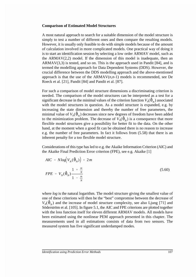
Considerations of this type has led to e.g. the Akaike Information Criterion (AIC) andthe Akaike Final Prediction Error criterion (FPE), see e.g. Akaike [1]

where log is the natural logarithm. The model structure giving the smallest value ofone of these criterions will then be the “best” compromise between the decrease ofV ( ) and the increase of model structure complexity, see also Ljung [71] andN

Söderström et al. [105]. In figure 5.1, the AIC and FPE criterions are plotted togetherwith the loss function itself for eleven different ARMAV models. All models havebeen estimated using the nonlinear PEM approach presented in this chapter. Themeasurements used in all estimations consists of data from two sensors. Themeasured system has five significant underdamped modes.

P( �N )

y( tk | tk1 ;� )

108 Summary

5.7.4 Model Validation

Model validation is the final stage of the system identification procedure. In factmodel validation overlaps with the model structure selection. Since systemidentification is, an iterative process various stages will not be separated, i.e. modelsare estimated and the validation results may lead to new models, etc. Modelvalidation involves two basic questions:

� What is the best model within the chosen model structure?� Is the model fit for its purpose?

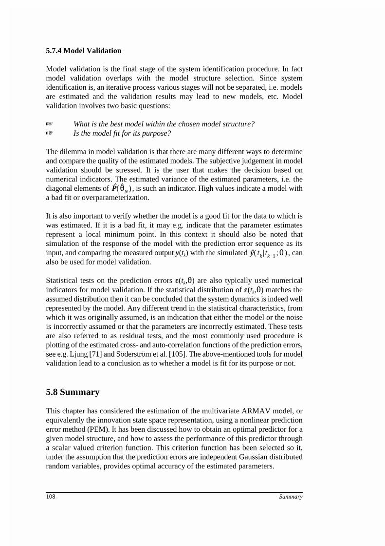
The dilemma in model validation is that there are many different ways to determineand compare the quality of the estimated models. The subjective judgement in modelvalidation should be stressed. It is the user that makes the decision based onnumerical indicators. The estimated variance of the estimated parameters, i.e. thediagonal elements of , is such an indicator. High values indicate a model witha bad fit or overparameterization.

It is also important to verify whether the model is a good fit for the data to which iswas estimated. If it is a bad fit, it may e.g. indicate that the parameter estimatesrepresent a local minimum point. In this context it should also be noted thatsimulation of the response of the model with the prediction error sequence as itsinput, and comparing the measured output y(t ) with the simulated , cank

also be used for model validation.

Statistical tests on the prediction errors �(t ,�) are also typically used numericalk

indicators for model validation. If the statistical distribution of �(t ,�) matches thek

assumed distribution then it can be concluded that the system dynamics is indeed wellrepresented by the model. Any different trend in the statistical characteristics, fromwhich it was originally assumed, is an indication that either the model or the noiseis incorrectly assumed or that the parameters are incorrectly estimated. These testsare also referred to as residual tests, and the most commonly used procedure isplotting of the estimated cross- and auto-correlation functions of the prediction errors,see e.g. Ljung [71] and Söderström et al. [105]. The above-mentioned tools for modelvalidation lead to a conclusion as to whether a model is fit for its purpose or not.

5.8 Summary

This chapter has considered the estimation of the multivariate ARMAV model, orequivalently the innovation state space representation, using a nonlinear predictionerror method (PEM). It has been discussed how to obtain an optimal predictor for agiven model structure, and how to assess the performance of this predictor througha scalar valued criterion function. This criterion function has been selected so it,under the assumption that the prediction errors are independent Gaussian distributedrandom variables, provides optimal accuracy of the estimated parameters.


The minimization of the criterion function, with respect to the adjustable parametersof the model structure, has then been investigated. A specific search scheme has beenconsidered. This is known as the Gauss-Newton search scheme for iterativeimprovement of an estimate. The statistical properties of the PEM estimator are thenconsidered. It is shown that if the true system is contained in the chosen modelstructure, and if the prediction error sequence is a white noise, then the estimator willbe consistent and asymptotically efficient. Based on these assumptions it is shownhow to obtain an estimate of the covariance of the estimated parameters. Finally,there is the problem of selecting the right model structure and how to validate thatthis model will actually fulfil its purpose. Practical guidelines for the selection of anappropriate and adequate model structure have been given.

5 identification using prediction error methods - svibs.com · 5 identification using prediction...

Documents