5. Linear Discriminant 5. Linear Discriminant FunctionsFunctions

ByBy

Ishwarryah S RamanathanIshwarryah S Ramanathan

Nicolette NicolosiNicolette Nicolosi

AgendaAgenda

�� 5.5 Minimizing Perceptron Criterion Function5.5 Minimizing Perceptron Criterion Function

–– The Perceptron Criterion FunctionThe Perceptron Criterion Function

–– Convergence Proof for Single Sample CorrectionConvergence Proof for Single Sample Correction

–– Direct GeneralizationsDirect Generalizations

�� 5.6 Relaxation Procedures5.6 Relaxation Procedures

–– The Descent AlgorithmThe Descent Algorithm

–– Convergence proofConvergence proof

�� 5.7 Non5.7 Non--Separable BehaviorSeparable Behavior

5.5 Minimizing the Perceptron 5.5 Minimizing the Perceptron Criterion FunctionCriterion Function

5.5.1 The perceptron criterion function5.5.1 The perceptron criterion function

�� Construct a criterion function for solving Construct a criterion function for solving linear equalities linear equalities aattyyii > 0.> 0.

�� The naive approach:The naive approach:

–– Let Let J(aJ(a; y; y11, ..., , ..., yynn) = number of samples ) = number of samples misclassified by a.misclassified by a.

–– This is a poor approach because the function This is a poor approach because the function is piecewise constant.is piecewise constant.

The perceptron criterion function contd.The perceptron criterion function contd.

�� A better choice is the A better choice is the Perceptron Perceptron

criterion functioncriterion function::

–– JJpp(a(a) = ) = ΣΣyyЄЄγγ ––aattyy

–– γγ(a(a) are the samples misclassified by a) are the samples misclassified by a

–– JJpp is 0 if no samples are misclassifiedis 0 if no samples are misclassified

Comparing Criterion FunctionsComparing Criterion Functions

Constructing the Perceptron AlgorithmConstructing the Perceptron Algorithm

�� The The jj--thth component of the gradient of component of the gradient of JJpp is is δδ JJpp / / δδ aajj. So,. So,

–– ∆∆JJpp = = ΣΣyyЄЄγγ ((--y)y)

�� This makes the update rule:This makes the update rule:

–– a(k+1) = a(k+1) = a(ka(k) + ) + ηη(k(k) ) ΣΣyyЄЄγγkk (y)(y)

–– γγkk is the set of samples misclassified by is the set of samples misclassified by a(ka(k))

The Batch Perceptron AlgorithmThe Batch Perceptron Algorithm

begin

init a, η(*), criterion θ, k = 0

do

k = k + 1

a = a + η(k)Σy•γk(y)

until | η(k)Σy•γk(y) | < θ

return a

end

The Batch Perceptron Algorithm contd.The Batch Perceptron Algorithm contd.

�� Basically, the next weight vector is determined Basically, the next weight vector is determined by adding the current weight vector to a by adding the current weight vector to a multiple of the number of misclassified samples.multiple of the number of misclassified samples.

�� The term The term batchbatch is used because a large number is used because a large number of samples are involved in computing each of samples are involved in computing each update.update.

�� Next slide: twoNext slide: two--dimensional example with a(1) = dimensional example with a(1) = 0 and 0 and ηη(k(k) = 1.) = 1.

Perceptron AlgorithmPerceptron Algorithm

5.5.2 Convergence Proof of 5.5.2 Convergence Proof of SingleSingle--Sample CorrectionSample Correction

Single Sample PerceptronSingle Sample Perceptron

�� Some simplifying assumptions:Some simplifying assumptions:

–– Modify the weight vector whenever a single sample in Modify the weight vector whenever a single sample in the sequence is misclassifiedthe sequence is misclassified

–– ηη(k(k) is constant ) is constant -- there is a fixed incrementthere is a fixed increment

–– yykk is a sample; is a sample; yykk is a misclassified sampleis a misclassified sample

–– This results in the This results in the fixedfixed--increment ruleincrement rule for for generating a sequence of weight vectors:generating a sequence of weight vectors:

�� a(1) arbitrarya(1) arbitrary

�� a(k+1) = a(k+1) = a(ka(k) + ) + yykk, where k >=1, where k >=1

FixedFixed--Increment Single Sample Perceptron AlgorithmIncrement Single Sample Perceptron Algorithm

begin

init a, k = 0

do

k = (k + 1) mod n

if yk is misclassified by a

then a = a + yk

until all patterns classified

return a

end

FixedFixed--Increment RuleIncrement Rule

Perceptron ConvergencePerceptron Convergence

�� If samples are linearly separable, then the If samples are linearly separable, then the previous algorithm will succeed and return previous algorithm will succeed and return a solution vector.a solution vector.

�� Idea:Idea:

–– If aIf a22 is any solution vector, then ||ais any solution vector, then ||a22(k+1) (k+1) --aa22|| is smaller than |||| is smaller than ||a(ka(k) ) -- aa22(k)||(k)||

–– True for many solution vectors, but not in True for many solution vectors, but not in general (see steps 6 and 7 in previous slide).general (see steps 6 and 7 in previous slide).

Perceptron Convergence contd.Perceptron Convergence contd.

�� We’ve already seen a(k+1) = We’ve already seen a(k+1) = a(ka(k) + ) + yykk. a. a22 is any is any solution vector such that asolution vector such that a22ttyyii is positive for all i. is positive for all i. We can add a scale factor We can add a scale factor αα and rewrite this and rewrite this equation: equation:

a(k+1) a(k+1) -- ααaa22= (= (a(ka(k) ) -- ααaa22) + ) + yykk

||a(k+1) ||a(k+1) -- ααaa22||||22 = ||= ||a(ka(k) ) -- ααaa22||||22 + 2(a(k) + 2(a(k) -- ααaa22))ttyykk + ||y+ ||ykk||||22

�� Because Because yykk was misclassified, was misclassified, aatt(k)yk(k)yk <= 0, <= 0, giving: giving:

||a(k+1) ||a(k+1) -- ααaa22||||22 <= ||<= ||a(ka(k) ) -- ααaa22||||22 + 2+ 2ααaa22ttyykk + ||y+ ||ykk||||22

Perceptron Convergence contd.Perceptron Convergence contd.

�� Because aBecause a22ttyykk is strictly positive, the is strictly positive, the second term will overpower the third term second term will overpower the third term if if αα is large enough.is large enough.

�� For example, let For example, let ββ be the maximum be the maximum pattern vector length ( pattern vector length ( ββ = max= maxii || || yyii ||||22 ), ), and and γγ be the smallest inner product of the be the smallest inner product of the solution vector with any pattern vector ( solution vector with any pattern vector ( γγ= min= minii [a[a22ttyyii] > 0 ).] > 0 ).

Perceptron Convergence contd.Perceptron Convergence contd.

�� We now have the inequality:We now have the inequality:||a(k+1) ||a(k+1) -- ααaa22||||22 <= ||<= ||a(ka(k) ) -- ααaa22||||22 -- 22αγαγ + + ββ22

�� Choosing Choosing αα = = ββ22//γγ gives:gives:||a(k+1) ||a(k+1) -- ααaa22||||22 <= ||<= ||a(ka(k) ) -- ααaa22||||22 -- ββ22

�� So, the squared distance between So, the squared distance between a(ka(k) and ) and ααaa22is reduced by at least is reduced by at least ββ22 after each correction. after each correction. After k corrections, we have:After k corrections, we have:||a(k+1) ||a(k+1) -- ααaa22||||22 <= ||a(1) <= ||a(1) -- ααaa22||||22 -- kkββ22

Perceptron Convergence contd.Perceptron Convergence contd.

�� The squared distance can not be negative, so there must The squared distance can not be negative, so there must be at most kbe at most k00 corrections, where kcorrections, where k00 = ||a(1) = ||a(1) -- ααaa22||||22 / / ββ22..

�� The weight vector that results after the corrections are The weight vector that results after the corrections are done must classify all samples correctly, because there done must classify all samples correctly, because there are a finite number of corrections that only occur at each are a finite number of corrections that only occur at each misclassification.misclassification.

�� In summary, kIn summary, k00 is a bound on the number of corrections, is a bound on the number of corrections, and there will always be a finite number of corrections and there will always be a finite number of corrections using the fixedusing the fixed--increment rule if the samples are linearly increment rule if the samples are linearly separable.separable.

5.5.3 Direct Generalizations5.5.3 Direct Generalizations

Variable Increment PerceptronVariable Increment Perceptron

�� A variant that uses a variable increment A variant that uses a variable increment ηη(k(k) and a margin b, and corrects when ) and a margin b, and corrects when aatt(k)y(k)ykk does not exceed the margin.does not exceed the margin.

�� The update function is now:The update function is now:a(1) arbitrarya(1) arbitrarya(k+1) = a(k+1) = a(ka(k) + ) + ηη(k)y(k)ykk k >= 1k >= 1

where where aatt(k)y(k)ykk <= b for all k<= b for all k

VariableVariable--Increment Perceptron ConvergenceIncrement Perceptron Convergence

�� It can be shown that It can be shown that a(ka(k) converges to a solution ) converges to a solution vector a satisfying vector a satisfying aattyyii > b for all i if the samples > b for all i if the samples are linearly separable and if: are linearly separable and if:

ηη(k(k) >= 0) >= 0

�� These conditions on These conditions on ηη(k(k) are satisfied if ) are satisfied if ηη(k(k) is a ) is a positive constant or decreases as 1/k.positive constant or decreases as 1/k.

VariableVariable--Increment Perceptron with MarginIncrement Perceptron with Margin

begin

init a, threshold ϴ, margin b, η(*), k

= 0

do

k = (k + 1) mod n

if atyk <= b

then a = a + η(k)yk

until atyk > b for all k

return a

end

Batch Variable Increment PerceptronBatch Variable Increment Perceptron

�� Another variant is the original gradient descent Another variant is the original gradient descent algorithm for algorithm for JJpp. The update function for this is:. The update function for this is:a(1) arbitrarya(1) arbitrarya(k+1) = a(k+1) = a(ka(k) + ) + ηη(k(k) + ) + ΣΣyyЄЄγγkk y , k >= 1y , k >= 1

�� It can be easily shown to return a solution. If aIt can be easily shown to return a solution. If a22is a solution vector, it correctly classifies the is a solution vector, it correctly classifies the correction vector: correction vector:

yykk = = ΣΣyyЄЄγγkk yy

Batch variable Increment Perceptron contd.Batch variable Increment Perceptron contd.

begin

init a, η(*), k = 0

do

k = (k + 1) mod n

γk = {}

j = 0

do j = j + 1

if yj is misclassified

then append yj to γkuntil j = n

a = a + η(k)Σy•γk(y)

until γk = {}

return a

end

Balanced Winnow AlgorithmBalanced Winnow Algorithm

�� Related to the Perceptron algorithm Related to the Perceptron algorithm -- the main the main difference is that the Perceptron algorithm returns a difference is that the Perceptron algorithm returns a weight vector with components weight vector with components aaii (i = 0, ..., d), and the (i = 0, ..., d), and the Winnow algorithm scales these by 2sinh[aWinnow algorithm scales these by 2sinh[aii].].

�� The balanced Winnow algorithm has separate positive The balanced Winnow algorithm has separate positive (a(a++) and negative (a) and negative (a--) weight vectors that are each ) weight vectors that are each associated with one of two categories to be learned. associated with one of two categories to be learned. Corrections to either only occur if a training pattern in its Corrections to either only occur if a training pattern in its own set is misclassified.own set is misclassified.

Balanced Winnow Algorithm contd.Balanced Winnow Algorithm contd.

begin

init a+, a-, η(*), k = 0, α > 1

if Sgn[a+tyk - a-tyk] != zk //misclassified

then

if zk = +1

then ai+ = α+yiai+; ai- = α-yiai- for all i

if zk = -1

then ai+ = α-yiai+; ai- = α+yiai- for all i

return a+, a-

end

Balanced Winnow Algorithm contd.Balanced Winnow Algorithm contd.

�� The main benefits of this version over the The main benefits of this version over the Perceptron algorithm are:Perceptron algorithm are:–– The two weight vectors move in a uniform direction The two weight vectors move in a uniform direction and the “gap” between them never increases. This and the “gap” between them never increases. This leads to a more general convergence proof than that leads to a more general convergence proof than that of the Perceptron.of the Perceptron.

–– Convergence is generally faster. This is because each Convergence is generally faster. This is because each weight does not go past the final value if the learning weight does not go past the final value if the learning rate is correctly set.rate is correctly set.

5.6 Relaxation Procedures5.6 Relaxation Procedures

5.6.1 The Descent Algorithm5.6.1 The Descent Algorithm�� We have the perceptron criterion functionWe have the perceptron criterion function

– Jp(a) = Σ y Є Ў (- aty) . . . Eq 1

– Ў is the set of training samples misclassified by ‘a’, the solution vector

�� Relaxation ProcedureRelaxation Procedure

– ‘Relaxation’ is a generalized approach to minimize the perceptron criterion function (eq 1) by linear classification.

– Jp(.) is a function with ‘a’ as a solution vector. Similar function Jq(.). Both denotes the misclassified sample.

The Descent Algorithm contd.The Descent Algorithm contd.–– JJqq(a(a) = ) = ΣΣ yyЄЎЄЎ (a(atty)y)2 2 . . . . . . EqEq 22

–– Adv: The curve is smoother (search is easier) and continuousAdv: The curve is smoother (search is easier) and continuous

–– There are two problems with this criterionThere are two problems with this criterion

�� The function is too smooth and slowly converge to a=0The function is too smooth and slowly converge to a=0

�� JJqq is dominated by training samples with large magnitudeis dominated by training samples with large magnitude

Fig.1 Jpp(a) Fig.2 Jqq(a)

[Taken from ‘Pattern Classification’ from Duda and Hart]

The Descent Algorithm contd.The Descent Algorithm contd.

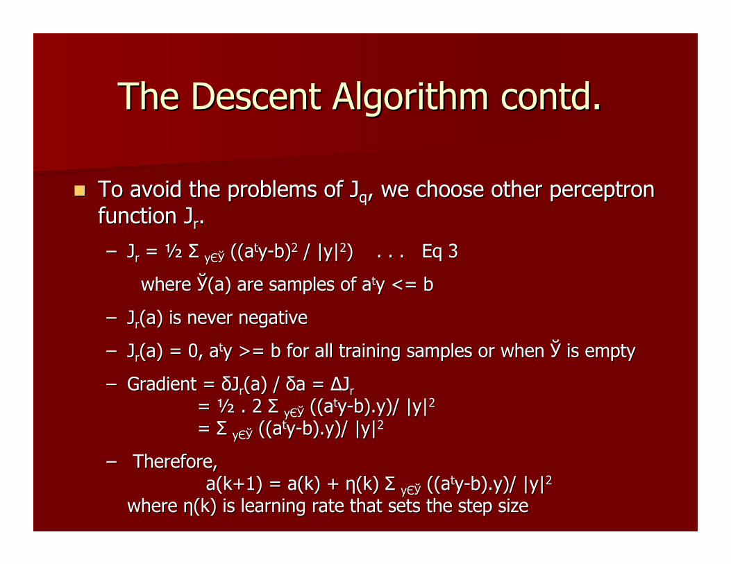
�� To avoid the problems of To avoid the problems of JJqq, we choose other perceptron , we choose other perceptron function Jfunction Jrr..

–– JJrr = ½ = ½ ΣΣ yyЄЎЄЎ ((a((attyy--b)b)22 / |y|/ |y|22) . . . ) . . . EqEq 33

where where ЎЎ(a) are samples of (a) are samples of aattyy <= b<= b

–– JJrr(a(a) is never negative) is never negative

–– JJrr(a(a) = 0, ) = 0, aattyy >= b for all training samples or when >= b for all training samples or when ЎЎ is emptyis empty

–– Gradient = Gradient = δδJJrr(a(a) / ) / δδa = ∆a = ∆JJrr= ½ . 2 = ½ . 2 ΣΣ yyЄЎЄЎ ((((aattyy--b).yb).y)/ |y|)/ |y|22

= = ΣΣ yyЄЎЄЎ ((((aattyy--b).yb).y)/ |y|)/ |y|22

–– Therefore, Therefore, a(k+1) = a(k+1) = a(ka(k) + ) + ηη(k) (k) ΣΣ yyЄЎЄЎ ((((aattyy--b).yb).y)/ |y|)/ |y|22

where where ηη(k) is learning rate that sets the step size(k) is learning rate that sets the step size

Batch Relaxation with MarginBatch Relaxation with Margin

begin

init a, η(*), b, k = 0

do k=(k+1) mod n

Yk = {}

j = 0

do j = j+1

if atyj <= b then append yj to Ykuntil j = n

a = a+ η(k) Σ yЄY ((b-aty).y) / |y|2

until Yk = {}

return a

end

Relaxation Algorithm contd.Relaxation Algorithm contd.

�� By SingleBy Single--Sample Correction Rule Sample Correction Rule analogous to analogous to EqEq 3,3,

–– a(1), a(1), arbitraryarbitrary

–– a(k+1) = a(k+1) = a(ka(k) + ) + ηη ((b((b--aatt(k).y(k).ykk).y).ykk) / |y) / |ykk||22 . . . . . . EqEq 4 4 where where aatt(k).y(k).ykk <= b for all k<= b for all k

SingleSingle--Sample Relaxation with MarginSample Relaxation with Margin

begin

init a, η(*), b, k = 0

do k=(k+1) mod n

if atyk <= b

then a=a+ η(k).((b-at(k).yk).yk)/|yk|2

until atyk > b for all yk

return a

end

Single Sample Relaxation RuleSingle Sample Relaxation Rule

�� Geometric Interpretation of SingleGeometric Interpretation of Single--Sample Relaxation Sample Relaxation RuleRule

–– r(kr(k) = () = (bb--aatt(k).y(k).ykk) / |) / |yykk||

–– r(kr(k) is the distance from the ) is the distance from the hyperplanehyperplane aattyykk=b to =b to a(ka(k).).

–– yykk / |/ |yykk| is the unit normal vector of | is the unit normal vector of hyperplanehyperplane

Geometric Interpretation of SingleGeometric Interpretation of Single--Sample Relaxation RuleSample Relaxation Rule

–– If If ηη=1, =1, a(ka(k) is moved to the ) is moved to the hyperplanehyperplane

–– EqEq 4 becomes,4 becomes,

aatt(k+1).y(k+1).ykk--b = (1b = (1--ηη) (a) (att(k).y(k).ykk -- b)b)

�� UnderUnder--RelaxationRelaxation

–– If If ηη<1 then a<1 then att(k+1).y(k+1).ykk is less than bis less than b

–– Slow descent or failure to convergeSlow descent or failure to converge

�� OverOver--RelaxationRelaxation

–– If If ηη>1 then a>1 then att(k+1).y(k+1).ykk is greater than bis greater than b

–– Overshoots, but convergence will finally be achievedOvershoots, but convergence will finally be achieved

�� Note: We restrict 0 < Note: We restrict 0 < ηη < 2< 2

5.6.2 Convergence Proof5.6.2 Convergence Proof

Convergence ProofConvergence Proof

�� Relaxation rule is on a set of Linearly Separable Relaxation rule is on a set of Linearly Separable Sample. The corrections may not be finiteSample. The corrections may not be finite

�� As the number of corrections goes to infinity we As the number of corrections goes to infinity we could see could see a(ka(k) converges to a limit vector on the ) converges to a limit vector on the boundary of the solution region.boundary of the solution region.

�� We can say region of We can say region of aattyy >= b is in the region of >= b is in the region of aattyy>0 if b>0>0 if b>0

�� Which implies that Which implies that a(ka(k) will enter this region) will enter this region

Convergence Proof contd.Convergence Proof contd.

�� ProofProof

–– Say ậ is any vector in solution regionSay ậ is any vector in solution region

–– ieie., ., ậậttyyii > b for all i then, > b for all i then, a(ka(k) gets closer to ậ at each step) gets closer to ậ at each step

–– From From EqEq 4, 4, ||a(k+1) ||a(k+1) -- ậ||ậ||22 = ||= ||a(ka(k) ) -- ậ||ậ||22 -- 22ηη ((((ậậ--a(k))a(k))ttyykk) (b) (b--aatt(k).y(k).ykk)/||y)/||ykk||||22

+ + ηη22 (b(b--aatt(k).y(k).ykk)2/||y)2/||ykk||||22

–– And (And (ậậ--a(k))a(k))ttyykk > > bb--aatt(k)y(k)ykk >= 0>= 0

–– So, So, ||a(k+1) ||a(k+1) -- ậ||ậ||22 <= ||<= ||a(ka(k) ) -- ậ||ậ||22 –– ηη(2 (2 -- ηη) (b) (b--aatt(k)y(k)ykk))22 / ||y/ ||ykk||||22

–– Because 0<Because 0<ηη<2, <2,

||a(k+1) ||a(k+1) -- ậ|| <= ||ậ|| <= ||a(ka(k) ) -- ậ||ậ||

–– Thus a(1),a(2),… gets closer to ậ and as limit k goes to infinitThus a(1),a(2),… gets closer to ậ and as limit k goes to infinity, ||y, ||a(ka(k) ) --ậ|| approaches a limiting distance ậ|| approaches a limiting distance r(ậr(ậ))

Convergence Proof contd.Convergence Proof contd.

–– That is, That is, a(ka(k) confines to a hyper) confines to a hyper--sphere of radius sphere of radius r(r(ậậ) with ậ as centre, ) with ậ as centre, as k goes to ∞.as k goes to ∞.

–– Therefore, Limiting Therefore, Limiting a(ka(k) is confined to intersect hyper) is confined to intersect hyper--spheres centered spheres centered about all of the possible solution vectors.about all of the possible solution vectors.

�� The intersection of the hyperThe intersection of the hyper--spheres is a single point on the spheres is a single point on the boundary of the solution region.boundary of the solution region.

–– Say a’ and a” are on the common intersection, then ||a’ Say a’ and a” are on the common intersection, then ||a’ -- ậ||=||a” ậ||=||a” -- ậ|| ậ|| for every ậ in the solution region.for every ậ in the solution region.

–– But ||a’ But ||a’ -- ậ||=||a” ậ||=||a” -- ậ|| implies that the solution region is contained in ậ|| implies that the solution region is contained in (d(d--1) dimensional hyper1) dimensional hyper--plane of points equidistant from a’ and a”.plane of points equidistant from a’ and a”.

–– But the solution region is d dimensional.But the solution region is d dimensional.

–– Which implies Which implies a(ka(k) converges to point ‘a’.) converges to point ‘a’.

Convergence Proof contd.Convergence Proof contd.

�� The point ‘a’ is not inside the solution The point ‘a’ is not inside the solution region because then the sequence would region because then the sequence would be finite.be finite.

�� It is not outside the region, because the It is not outside the region, because the correction will make ‘a’ move correction will make ‘a’ move ηη times its times its distance from boundary plane.distance from boundary plane.

�� Therefore, Therefore, the limit point must be on the the limit point must be on the boundaryboundary..

5.7 Non5.7 Non--separable behaviorseparable behavior

�� The Perceptron and Relaxation procedures are methods The Perceptron and Relaxation procedures are methods for finding a separating vector when the samples are for finding a separating vector when the samples are linearly separable. They are linearly separable. They are error correctingerror correcting proceduresprocedures

�� Separating Vector in training does not mean the Separating Vector in training does not mean the resulting classifier will perform well on independent test resulting classifier will perform well on independent test datadata

�� For performance, many training samples should be usedFor performance, many training samples should be used

�� Sufficiently large training samples are almost certainly Sufficiently large training samples are almost certainly not linearly separablenot linearly separable

�� No weight vector can correctly classify every sample in a No weight vector can correctly classify every sample in a nonnon--separable setseparable set

5.7 Non5.7 Non--separable Behavior contd.separable Behavior contd.

�� Number of corrections in the Perceptron and Number of corrections in the Perceptron and Relaxation procedures goes to infinity if set is Relaxation procedures goes to infinity if set is nonnon--separableseparable

�� Performance improves if Performance improves if ηη(k)(k)-->0 as k>0 as k-->>∞∞

�� The rate at which The rate at which ηη(k) (k) approaches zero is approaches zero is important: important:

–– Too slow: Too slow: Results will be sensitive to those training Results will be sensitive to those training samples that render the set nonsamples that render the set non--separable. separable.

–– Too fast: Too fast: Weight vector may converge prematurely Weight vector may converge prematurely with less than optimal results.with less than optimal results.

Research IdeasResearch Ideas

�� Paper by Paper by Khardon and Wachman discusses Khardon and Wachman discusses performance of variants of the Perceptron performance of variants of the Perceptron algorithm.algorithm.–– They discovered that the variant that uses a margin They discovered that the variant that uses a margin has the unintended side effect of tolerating noise and has the unintended side effect of tolerating noise and stabilizing the algorithm.stabilizing the algorithm.

–– The authors implemented several variants of the The authors implemented several variants of the algorithm and performed experiments using different algorithm and performed experiments using different sets of data to compare performance.sets of data to compare performance.

–– Good overview of a practical implementation and its Good overview of a practical implementation and its results.results.

Research IdeasResearch Ideas

�� Paper by Paper by S. J. Wan on Cone Algorithm –Extension to Perceptron Algorithm

– Perceptron convergence is important in machine learning algorithms

– Find a covering cone for a finite set of linearly contained vectors and the convergence

– Theorems, definitions and equations are well defined.

ReferencesReferences

�� Pattern Classification, 2nd ed by Pattern Classification, 2nd ed by DudaDuda R, Hart P, R, Hart P, Stork D, 2001. John Wiley Stork D, 2001. John Wiley & Sons.& Sons.

�� Noise Tolerant Variants of the Perceptron Noise Tolerant Variants of the Perceptron Algorithm by R. Khardon and G. Wachman Algorithm by R. Khardon and G. Wachman --Journal. Mach. Learn. Res. Pg 227Journal. Mach. Learn. Res. Pg 227--248 May2007248 May2007

� Cone Algorithm: An Extension of the Perceptron Algorithm by S. J. Wan - IEEE Transactions on Systems, Man and Cybernetics, Vol. 24, No. 10, October 1994

THANKS!THANKS!