53244919 flexural comparison of the aci 318 08 and aashto lrfd structural
TRANSCRIPT
San Jose State UniversitySJSU ScholarWorks
Master's Theses Master's Theses and Graduate Research
2008
Flexural comparison of the ACI 318-08 andAASHTO LRFD structural concrete codesNathan Jeffrey DorseySan Jose State University
This Thesis is brought to you for free and open access by the Master's Theses and Graduate Research at SJSU ScholarWorks. It has been accepted forinclusion in Master's Theses by an authorized administrator of SJSU ScholarWorks. For more information, please contact [email protected].
Recommended CitationDorsey, Nathan Jeffrey, "Flexural comparison of the ACI 318-08 and AASHTO LRFD structural concrete codes" (2008). Master'sTheses. Paper 3562.http://scholarworks.sjsu.edu/etd_theses/3562

FLEXURAL COMPARISON OF THE ACI 318-08 AND AASHTO LRFD STRUCTURAL CONCRETE CODES
A Thesis
Presented to
The Faculty of the Department of Civil Engineering
San Jose State University
In Partial Fulfillment
of the Requirements for the Degree
Master of Science
by
Nathan Jeffrey Dorsey
May 2008
UMI Number: 1458121
Copyright 2008 by
Dorsey, Nathan Jeffrey
All rights reserved.
INFORMATION TO USERS
The quality of this reproduction is dependent upon the quality of the copy
submitted. Broken or indistinct print, colored or poor quality illustrations and
photographs, print bleed-through, substandard margins, and improper
alignment can adversely affect reproduction.
In the unlikely event that the author did not send a complete manuscript
and there are missing pages, these will be noted. Also, if unauthorized
copyright material had to be removed, a note will indicate the deletion.
®
UMI UMI Microform 1458121
Copyright 2008 by ProQuest LLC.
All rights reserved. This microform edition is protected against
unauthorized copying under Title 17, United States Code.
ProQuest LLC 789 E. Eisenhower Parkway
PO Box 1346 Ann Arbor, Ml 48106-1346

©2008
Nathan Jeffrey Dorsey
ALL RIGHTS RESERVED

APPROVED FOR THE DEPARTMENT OF CIVIL ENGINEERING
j/jfl^L-Dr. Akthem Al-Manaseer
Dr. Kurt M. McMullin
1 Mr. Daniel Merrick
APPROVED FOR THE UNIVERSITY
£<? / Au0Lr~**~~ Vi/zo/os'

ABSTRACT
FLEXURAL COMPARISON OF THE ACI 318-08 AND AASHTO LRFD STRUCTURAL CONCRETE CODES
by Nathan Jeffrey Dorsey
There are two prevailing codes utilized during the design of structural concrete
members in North America, ACI 318-08 and AASHTO LRFD. Each takes a unique
approach to achieve the same result, a safe working design of a structural concrete
section; however there are fundamental differences between the codes regarding the
calculation of member properties.
The purpose of this paper was to investigate these differences between codes
encountered during the calculation of flexural strength or moment capacity of a section.
This study focused on the code's influence during the classical approach to analysis of a
shallow reinforced T-beam and the strut and tie model method as applied to a series of
deep beams with openings. Parametric studies were conducted using software developed
by the author specifically for this purpose.
It was concluded that both codes provided similar and safe results regardless of
the very different approaches to solution taken by each.

ACKNOWLEDGEMENTS
I would like to thank Dr. Akthem Al-Manaseer for his patience and support
during this process. Dr. Al-Manaseer gave me full academic freedom during the course
of this research and by doing so provided me with a tremendous learning experience that
went far beyond reinforced concrete.
And I would especially like to thank my lovely wife Jaya for always believing in
me and for making sure that I always believed in myself.
v

Table of Contents 1.0 INTRODUCTION 1
1.1 General 1 1.2 Scope 1 1.3 Objective 1 1.4 Outline 2
2.0 LITERATURE REVIEW 3 2.1 Introduction 3 2.2 Shallow Beams 4 2.3 Deep Beams 24
3.0 THEORY OF FLEXURE 37 3.1 Background 37 3.2 Theory of Flexure in Shallow Reinforced Concrete Sections 39 3.3 Theory of Flexure in Deep Beams 43
4.0 ANALYTICAL PROCEDURE 48 4.1 Shallow Beams 48
4.1.1 Stress Block Depth Factor^ 50 4.1.2 ACI 318-08 51
4.1.2.1 Limits of Reinforcement 51 4.1.2.2 Location of Neutral Axis c and Depth of Compressive Block a 52 4.1.2.3 Strength Reduction Factor ^ 54
4.1.3 AASHTO LRFD 59 4.1.3.1 Limits of Reinforcement 59 4.1.3.2 Location of Neutral Axis c, and Depth of Compressive Block a 60 4.1.3.3 Strength Reduction Factor <f> 62
4.2 STM 66 4.2.1 Introduction 66
4.2.1.1 Graphical Solution 69 4.2.1.2 Hand Calculations 70 4.2.1.3 Excel Spreadsheets 70
4.2.2 ACI 318-08 vs. AASHTO LRFD 72 4.2.3 Strength Reduction Factor <j> 72 4.2.4 Strut Effectiveness Factors f3s 73 4.2.5 Node Effectiveness Factors f3„ 73
5.0 RESULTS and DISCUSSION 76 5.1 Flexure 76
5.1.1 Asmin m&Asmax, ACI 318-08 versus ASHTO LRFD 77 5.1.2 As versus Mu 83 5.1.3 Location of Neutral Axis c, and Depth of Compressive Block a 90 5.1.4 Strength Reduction Factor ^ 92
5.2 STM 98 5.2.1 Maximum Allowable Concentrated Load - STM versus FEA 99
vi

5.2.2 Maximum Allowable Concentrated Load without $- STM versus FEA 100
6.0 SUMMARY and CONCLUSIONS 103 6.1 Summary 103 6.2 Conclusion 104
6.2.1 Asmin and Asmax for Flexure 104 6.2.2 As versus Mu for Flexure 104 6.2.3 Depth of Neutral Axis c for Flexure 104 6.2.4 Strength Reduction Factor <f> for Flexure 105 6.2.5 Maximum Load Capacityfor STM 105
Works Cited 106 Appendix A - Deep Beam STM Models 108 Appendix B - Deep Beam STM Truss Models 113 Appendix C - STM Truss Free Body Diagrams & Solutions 119
vii

List of Figures Figure 2-1 AASHTO LRFD Procedure for calculation of sx 7 Figure 2-2 Summary of reinforcement limits by 1999, 2002 ACI codes and AASHTO LRFD and Naaman recommendation 18 Figure 2-3 ACI 318-05 and AASHTO LRFD limits of reinforcement 22 Figure 3-1 Beam in flexure with saddling effect 38 Figure 3-2 Graphic representation of forces within a reinforced concrete section 42 Figure 3-3 ACI 318-08 Fig. RA.1.1 (a and b) - D-regions and discontinuities 45 Figure 3-4 ACI 318-08 Fig. RA.1.5 (a and b) - Hydrostatic nodes 47 Figure 4-1 Section geometry 49 Figure 4-2 IF logic statement for computation of stress block depth factor /?/ 50 Figure 4-3 ACI 318-08 Fig. R9.3.2 - Strength reduction factor 54 Figure 4-4 ACI 318-08 calculation of strength reduction factor ^ 55 Figure 4-5 Sample excel spreadsheet analysis 56 Figure 4-6 Sample excel spreadsheet showing preliminary ACI 318-08 calculations 57 Figure 4-7 ACI 318-08 excel program logic flowchart 58 Figure 4-8 Determination of AASHTO LRSYi Asmca 62 Figure 4-9 AASHTO LRFD and ACI 318-08 limits of reinforcement 63 Figure 4-10 Sample excel spreadsheet for AASHTO LRFD analysis 64 Figure 4-11 AASHTO LRFD flowchart 65 Figure 4-12 Generic beam with and without opening 67 Figure 4-13 Strut and tie modeling procedure 75 Figure 5-1 Graphic representation of section geometry 76 Figure 5-2 Asmax andAsmin as a function of b 79 Figure 5-3 Asmax andAsmin as a function of bw 80 Figure 5-4 Asmax and Asmi„ as a function of d 81 Figure 5-5 Asmax and Asmin as a function of tf 82 Figure 5-6 As versus Mu for variable b 86 Figure 5-7 As versus Mu for variable bw 87 Figure 5-8 As versus Mu for variable d 88 Figure 5-9 As versus Mu for variable tf 89 Figure 5-10 As versus c for variable b 94 Figure 5-11 4* versus c for variable bw 95 Figure 5-12 As versus c for variable d 96 Figure 5-13 As versus c for variable tf 97 Figure 5-14 Generic beam with and without opening 98 Figure 5-15 Predicted load vs. maximum test load comparisons 102 Figure 5-16 Predicted load without ^ vs. maximum test load comparisons 102
viii

List of Tables Table 4-1 Values for variable and fixed geometry for each case 49 Table 4-2 Cutout locations from lower left corner in inches 67 Table 4-3 ACI 318-08/AASHTO LRFD effective strength coefficients 74 Table 5-1 Rates of change for ACI 318-08 and AASHTO LRFD Asmin and Asmax 77 Table 5-2 Ratio of AASHTO LRFD to ACI 318-08 for Mu per unit A, 83 Table 5-3 Results for location of neutral axis 91 Table 5-4 Cutout locations from lower left corner in inches 98 Table 5-5 Predicted load versus maximum test load comparisons 99 Table 5-6 Predicted load without ^versus maximum test load comparisons 101
ix

List of Variables
a effective depth of the compressive block a' distance from center of concentrated load to edge of support Ac' area of concrete on flexural compression side of member Aps area of prestressed longitudinal reinforcement placed on the flexural tension side
of the section As area of flexural reinforcement As area of non-prestressed longitudinal reinforcement placed on the flexural tension
side of the section As area of conventional non-prestressed tensile reinforcing steel As' area of conventional non-prestressed compressive reinforcing steel Av cross sectional area of provided stirrup reinforcement within distance s b section width bv effective web width bw web width c distance from extreme compressive fiber to neutral axis d distance from the extreme compressive fiber to the centroid of the flexural
reinforcement D overall member depth dc strut width de depth from the extreme compressive fiber to the centroid of the tensile force in the
non-prestressed reinforcement, i.e. reinforcing bars also called the effective depth of main flexural reinforcement
d„ effective shear depth, can be taken as 0.9d dp depth from the extreme compressive fiber to the centroid of the tensile force in the
prestressed reinforcement ds depth from the extreme compressive fiber to the centroid of the tensile force in the
non-prestressed reinforcement, i.e. reinforcing bars dv effective shear depth, taken as 0.9d E modulus of elasticity of the material, commonly referred to as Young's Modulus Ec elastic modulus of concrete Ep modulus of elasticity of prestressed reinforcement Es modulus of elasticity of non-prestressed reinforcement f*c effective concrete strength f'c compressive concrete strength fps stress in the prestressing steel at nominal bending resistance fpu tensile strength of prestressing steel fsy yield strength of main longitudinal reinforcing steel fy yield strength of conventional non-prestressed reinforcing steel kz ratio of the in situ strength to the cylinder strength Mu factored moment; taken as a positive quantity not less than Vud„ n efficiency factor Nu factored axial force; positive if tensile, negative if compressive
x

s stirrup spacing tf flange thickness Tu factored torsion V shear force Vc shear strength contribution from concrete Vs shear strength contribution from reinforcing steel Vu factored shear w node width over which shear force is applied z distance between node centers s strain
Si major principal strain, normal to strut £2 minor principal strain, parallel to strut
Ex strain in the horizontal direction
Q equivalent strut width over which ties contribute
9 angle of strut to horizontal
6 angle of strut to longitudinal axis
6 a stress
xi

1
1.0 INTRODUCTION
1.1 General
The purpose of this thesis is to compare and contrast the ACI 318-08 and the
AASHTO LRFD 3rd Ed. code provisions and design philosophies.
1.2 Scope
The crux of this thesis is the comparison of the two prevailing concrete design
codes regarding the design and detailing of concrete beams in pure flexure with no other
loading present. The discussion on shallow beams used a series of twelve flanged beams
as its focus while the deep beam discussion focused on a series of five deep beams and
the Strut-and-Tie Model (STM) method. To accomplish this a series of Excel
spreadsheets were created to ensure the accuracy and consistency of all calculations
performed; however as programming is not the point of this research several simplifying
assumptions were made to reduce the time required to create, vet and utilize these tools.
Both sections focus solely on analytical results; no laboratory experiments were
carried out. Comparisons were based on but not limited to maximum predicted allowable
load.
1.3 Objective
The objective of this thesis is to clarify the differences between the two prevailing
concrete design codes, ACI 318-02 and AASHTO LRFD 3rd Ed. and categorize them as

2
major, minor, or insignificant. For simplicity when the AASHTO LRFD 3r Ed. is
referenced, the 3rd Ed. shall be omitted. In cases where other editions are referenced, the
edition under discussion shall be noted. An additional comparison will be made between
the results produced by the two codes when using the method of STM and the actual
experimental test loads used during experimental work carried out by Ha in 2002. A
comprehensive literature review providing coverage of examples illustrating additional
differences found between the ACI 318 and AASHTO LRFD codes beyond pure flexure
and deep beams is included.
1.4 Outline
Chapter 2 contains a literature review of relevant academic and industry articles
regarding a specific structural member type, a specific concrete design code or a
comparative study of both codes. Chapter 3 provides a brief introduction and review of
the design philosophy of both flexural analysis for shallow reinforced concrete beams and
the STM method of design for reinforced concrete deep beams. Chapter 4 details the
analytical procedure as described by each code and what methods were implemented by
the software tools developed. Chapter 5 contains the results obtained from this study.
Chapter 6 provides the concluding remarks on the findings of this study.

3
2.0 LITERATURE REVIEW
2.1 Introduction
The flexural resistance or moment capacity of a structural member is a
fundamental part of the overall analysis required when designing or evaluating an
assembly of structural concrete sections. This flexural resistance is only one of a myriad
offerees that needs to be considered when designing or evaluating a structural member.
Other forces due to direct loading or reactions such as axial, torsional and shear forces
must not be overlooked.
Of the many comparisons between the American Concrete Institute (ACI) 318
Building Code Requirements for Structural Concrete and the American Association of
State Highway Transport Officials Load and Resistance Factor Design (AASHTO LRJFD)
Bridge Design Specifications for non-prestressed concrete members reviewed only one
article directly addressed differences when analyzing or designing a structure with
respect to the flexural resistance. However many of the conclusions presented by the
reviewed articles followed the same general trend.
Articles detailing differences in method and results when using the strut-and-tie
model (STM) method were rather numerous and articles reviewed or discussed in this
paper date back as far as 1996, older articles on these subjects were available but were
not considered for review due to the significant revisions made to the codes since the
time of publication.

4
2.2 Shallow Beams
Gupta and Collins (537-47) performed a study that primarily focused on the
question of the safety of using traditional shear design procedures based on the failure of
the Sleipner offshore platform on 23 August, 1991. To aid in their determination of the
safety of these traditional methods of analysis and design 24 reinforced concrete elements
having concrete compressive strengths ranging from 4280 to 12,600 psi were loaded
under a variety of shear and compressive axial load combinations. The results from these
tests were used to evaluate the design provisions of the ACI 318-99 and AASHTO LRFD
"Bridge Design Specifications and Commentary " 2" Ed.
The ACI 318-99 code provisions made a general assumption that the shear stress
of a member V„, could be defined as the sum of the shear load at which diagonal cracks
form Vc, and the provided shear capacity of any stirrups present using the traditional 45
degree truss equation, Vs.
V„=K+VS (2-1)
The traditional 45 degree truss equation is defined as
VS=^IA (2-2) s
The code also allowed for a simplified conservative calculation to be used for Vc
although the detailed approach provided for more accurate and less conservative results.
Both equations are shown below. The simplified and conservative approach is detailed in

5
Equation 2.3 while the detailed approach is shown in Equation 2.4. Both equations
require the use of English units.
V.'„ = 2 1 + -N..
20004. rxd (2-3)
1.9^77 + 2500^-^V* (2-4)
Nu in Equation 2-3 represents the load due to axial compression and Mm in Equation 2-4
represents the modified moment as defined by the relationship shown in Equation 2-5.
'Ah-d^ Mm=Mu-Nu 8
(2-5)
Regardless of the method utilized for calculation of the shear load at which
diagonal cracks form the ACI 318-99 code placed a restriction on the maximum value for
Vc as defined by
Vc<3.54JrXdfi + N„
5004. (2-6)
These detailed equations for Vc were derived by ACI-ASCE Committee 326 in
1962 and were based on the principal stress as found at the location of the diagonal
tension cracking.
The AASHTO LRFD shear design procedure did not use the general assumptions
utilized by the ACI 318-99 provisions, rather it relied on the more involved modified
compression field theory (MCFT) which in turn uses relationships between equilibrium,

6
compatibility and stress and strain to predict the shear capacity of cracked concrete
section/elements. In addition to the obvious difference between the backgrounds of the
two code provisions note that the AASHTO LRFD used SI units of MPa whereas the ACI
318-99 provided solutions in English units of psi.
Hence the AASHTO LRFD expression for shear resistance of a section, V„, was
more involved and incorporated several different sub-equations. AASHTO LRFD
defined shear resistance as
Vn = 0.0830Jf\bvdv + - ^ d v cot0 (MPa) (2-7)
s
The variables were defined as:
Av = cross sectional area of provided stirrup reinforcement within
distance s
bv = effective web width
dv = effective shear depth, taken as 0.9d
f'c = compressive strength of concrete
fy = yield stress of steel reinforcement
s = stirrup spacing
Values for /?and 6 were derived from calculating the stresses transmitted across
diagonal cracked concrete sections which contained no less than the minimum required

7
transverse reinforcement for crack control. This minimum amount of transverse
reinforcement Av>mi„, was defined and calculated by AASHTO LRFD as
<mi„ = 0.083V77^ (MPa) J y
(2-8)
The values for /? and 9 were dependant on the shear stress, v, and the longitudinal
mid-depth strain of the section, sx. Figure 2-1 details the idealized section used by
AASHTO LRFD in the calculation of sx for this procedure.
A's A< \ Flanged Compression
\ \ / Section
» • %\ M
-^ +0.57V -0.5F,cot^
d. N, V„
•-*_
/ f \ Ac A<i Flanged Compression
Section Idealized Section
^
Flanged Forces, dv
Web Forces and Section Forces
Vcoid
0.5N+Q.5Vcoi6
Longitudinal Strains
Figure 2-1 AASHTO LRFD Procedure for calculation of ex
Mathematically the longitudinal mid-depth strain of this section is defined by the
relationship shown in Equation 2-9.
£•„ = e,sc (2-9)
Where the terms s, represented the longitudinal tensile strain in the flexural tension flange
and ec represented the longitudinal compressive strain in the flexural compressive flange.

8
Mathematically st and sc were calculated as shown in Equations 2-10 and 2-11.
^*—0.5N+0.5F cot<9 7 U U
£ i = _ l ( 2 . 1 0 )
^± + Q.5N -0.5V, cote 7 U U
£ = Ji ( 2 . i i )
EA + EA'
The newly introduced variables were defined as:
Ac' = area of concrete on flexural compression side of member
Ec = elastic modulus of concrete
Es - elastic modulus of steel
And Kwas defined by the relationship shown in Equation 2-12.
v = ^~ (2-12)
The result of the relationships defined above was that for an increase in axial
compression the variables Nu, sx and # decreased while /? would increase. This
contributed to an increased shear capacity for any given section.
In order to obtain empirical data to corroborate the analytical predictions from
each code's procedure a series of 24 specimens were built and tested in the University of
Toronto's shell element testing apparatus. Specimens were designed to represent the

9
sections of a structural wall that was simultaneously subjected to high axial compression
and high out of plane shear loads.
Specimen length L, overall section depth h, total percentage of longitudinal
reinforcement px, and total percentage of transverse reinforcement across the specimen
width py were not varied during the course of investigation. The parameters that were
variable were the compression to shear ratio N/V, the concrete compressive strengthf'c,
specimen width b and the shear reinforcement provided r:.
Loads were induced by five series of six jacks that applied pressure onto steel
transfer beams located on the top and bottom faces of the specimens. A compressive
stress of up to 9400 psi was applied along with equal but opposite moments applied to
each end of the specimen bending it in double curvature. In each test case the loads from
axial, shear and moments were increased proportionally until the specimens reached
failure. Tangential deformation was used as the means of quantifying the total
deformation of each specimen.
Strains from the flexural tension side of the member ext and the flexural
compression side of the member sxc, were measured from locations directly adjacent to
the steel end plates. Strain for the shear reinforcement was measured directly from the T-
headed bars used to provide shear reinforcement and reinforcement across the member
width.

10
Failures were classified as shear S, or flexural F, based on the observed strains in
the Ext and sxc directions at the ends of the specimen when compared to the magnitude of
the applied moment at the specimen ends ME and the shear strains yx:. Of the 24
specimens tested 18 were classified as failing in shear while the remaining 6 were
classified as flexural failures. In the six flexural failures it was determined that the
longitudinal reinforcement yielded and the applied moment ME, approximately equaled or
exceeded the predicted moment at failure M0.
This experiment demonstrated that when the ACI 318-99 conservative method for
calculating Vc was utilized the shear strength and mode of failure for a reinforced
specimen loaded under high axial compression can be consistently predicted; whereas
when using the more detailed method of calculating Vc was used, the mode of failure can
be brittle shear and occur at loads significantly less than those predicted, on average 68%
less. It was demonstrated that it was possible to properly design a section using the
detailed method described by this procedure and yet only provide a factor of safety as
low as 1.10.
The AASHTO LRFD procedure for calculating Vc provided far more accurate and
consistent results for shear failure and the upper limit of shear capacity as induced by an
increase in axial compression was correctly predicted.

11
Two major recommendations arose from these results:
• The detailed expression for Vc be removed from the ACI 318 code
• The term for axial compression NJAS in Equations 2-3 and 2-6 not be
taken greater than 3000 psi
Rahal and Collins (277-82) undertook research to provide an evaluation of the
design provisions for combined shear and torsion load cases as described by both the ACI
318-02 and the AASHTO LRFD Bridge Design Specifications, 2nd Edition.
When Rahal and Collins' report was published the current version of each code
contained torsional design provisions that were similar other than the method used to
determine the angle 6. Rahal and Collins noted that the AASHTO LRFD provisions had
been extensively checked for shear cases whereas the ACI 318-02 provisions had been
extensively checked for pure torsion as well as combined torsion and bending. It was
concluded that there was a lack of data available that directly correlated the torsional
provisions of each code. Hence Rahal and Collins ran four large scale experiments to
compare the results of the calculated torsion-shear interaction diagrams obtained from
both the AASHTO LRFD and ACI 318-02 provisions. The beams tested were solid,
rectangular sections 340mm wide and 640mm deep reinforced with non-prestressed
longitudinal bars.
The ACI 318-02 code described the basic truss equation relating the provided
hoop reinforcement to torsional strength as follows:

12
T„ = 2A0 - ^ cot 9 (SI Units) (2-13)
s
Where A0 represented the area enclosed by the shear flow path and was permitted
to be taken as 0.85*Aoh, and where A0h represented the area enclosed by the outermost
transverse torsional reinforcement. fyv was the yield strength of the hoop reinforcement and At represented the cross sectional area of one leg of the transverse reinforcement. 0
represented the angle of inclination of the compressive diagonals and was noted to have
rather ambivalent instructions to its suggested versus its analyzed values. As described in
ACI 318-02 §11.6.3.6 the angle 6shall not be less than 30 degrees but it is suggested that
<9= 45 degrees for non-prestressed members and 6= 37.5 degrees for members that are
prestressed.
A similar truss equation, see Equation 2-14, related the torsional strength to the
quantity of longitudinal reinforcement provided.
A f T„=2A0 -!+*- tan 3 (SI Units) (2-14)
Ph
Rahal and Collins observed that when comparing equations 2-13 and 2-14 the
equivalent torsional strengths could be obtained by using less hoop reinforcement but
increasing the longitudinal reinforcement.

13
When these two equations were set equal to each other the required area of
transverse reinforcement could be solved for as shown by Equation 2-15.
A f Al=^-Ph^cot20 (SI Units) (2-15)
s fyt
The ACI 318-02 equation for a non-prestressed section that described the
relationship between transverse reinforcement and shear strength is shown in Equation 2-
16.
K = K + K= 0A66j]\bwd + - ^ d (MPa) (2-16)
The variables were defined as:
As = area of flexural reinforcement
bw - web width
d = distance from the extreme compressive fiber to the centroid of the flexural
reinforcement
f'c = compressive concrete strength
fy = yield strength of reinforcing steel
Vc - shear strength contribution from concrete
Vs = shear strength contribution from reinforcing steel
Additionally the ACI 318-02 code required that the nominal shear stress for solid
sections be limited to avoid concrete crush prior to reinforcement yield. Equation 2-17
describes this limitation.

14
v^2 f
bJj - ^ r < 0.83SK (SI Units) (2-17)
The AASHTO LRFD code used the same basic truss equation as the ACI 318-02,
Equation 2-13, to relate the area of one leg of the transverse reinforcement^,, to the
required torsional strength T„. However the AASHTO LRFD relationship between the
minimum required shear strength V„ and the required area of transverse reinforcement Av
was noticeably different from that shown for ACI 318-02 in Equation 2-18.
V = Vc + Vs = 0.083£ Jf~cbvdv +—< cot 9 (SI Units) (2-18) s
The variable bv represented the web width, however dv was defined as the
effective shear depth which can be taken as 0.9*d. For sections containing stirrups the
values for J3 and # depended on the nominal shear stress v, and the mid-depth
longitudinal strain ex.
Rahal and Collins noted that when /?was set equal to 2.22 the AASHTO LRFD
value matched the ACI 318-02 value for Vc exactly. Also when examining non-
prestressed sections sx could be taken as 1.00x10" which provided a value of 36 degrees
for 0, and when the AASHTO LRFD value for 6 equaled 36 degrees the results for Vs
were 24% higher than those obtained from the ACI 318-02 procedure.

15
Equation 2-19 details the nominal shear stress v, for a solid section as calculated
under the AASHTO LRFD provisions for a solid section under combined shear and
torsion which was required to be no greater than 0.25/'c to avoid failures due to concrete
crushing.
PA j
2 (T
A 2
\Aoh J
<0.25/'c (MPa) (2-19)
The longitudinal stress sx, at the mid-plane could be taken as l.OOxlO'3 or it could
be calculated using the relationship shown in Equation 2-20.
M. 2 !L + 0.5N„ + 0.5 cot 6JV„ + 0-Wu
2(EsAs + EpAps)
"0.7/aA £x = -1 ' v 2f° J (2-20)
Variables in Equation 2-20 were defined as:
As = area of non-prestressed longitudinal reinforcement placed on the flexural
tension side of the section
Aps - area of prestressed longitudinal reinforcement placed on the flexural tension
side of the section
dv= effective shear depth, can be taken as 0.9d
Es = modulus of elasticity of non-prestressed reinforcement
Ep = modulus of elasticity of prestressed reinforcement
fpu = tensile strength of prestressing steel
Mu = factored moment; taken as a positive quantity not less than Vudv

16
Nu = factored axial force; positive if tensile, negative if compressive
Tu = factored torsion
Vu = factored shear
Rahal and Collins noted that for prestressed sections sx would often approach
zero. In these cases the value of 6 would vary from 22 to 30 degrees depending on the
level of shear stress present.
The AASHTO LRFD provisions required that the tensile capacity of the
longitudinal reinforcement on the flexural tension side of the section be no less than the
force TE, to prevent premature failure of the longitudinal reinforcement. TE was
calculated as shown in Equation 2-21.
fir V / / W C T - V
M . <i> \\<t> ) \ <t>1Ao j
WJMM (2-21)
The test variable in the series was the torsion to shear ratio which varied from
zero to 1.216m. Specimen failures were attributed to excessive yielding of the closed
stirrups as well as spalling and crushing of the concrete in the test region.
Rahal and Collins determined that use of the ACI 318-02 provisions produced
very conservative results when the maximum value of 45 degrees for the angle of the
compression diagonals 6, was used. Conversely when the minimum value for #of 30
17
degrees was used the ACI 318-02 provisions demonstrated less consistent results and
provided failure loads for high torsion-to-shear ratios much higher than those observed.
Results obtained from use of the AASHTO LRFD provisions provided a
consistent value of approximately 36 degrees for 6. Use of this value provided results of
a consistent and reasonable nature that closely replicated the observed crack patterns.
Naaman (209-18) investigated the differences between the ACI 318-02 and
AASHTO LRFD codes regarding sections that were classified as being between tension
controlled and compression controlled, i.e. in the transition zone. Naaman found and
described several examples where the ACI 318-02 provisions regarding the limits of
reinforcement for flexural members lead to unintended erroneous results that brought the
validity of the provision into question. These flaws were not directly correlated to the
corresponding AASHTO LRFD provisions but they did reflect similar results for other
ACI provisions as described by several other publications where solutions appeared
conservative but in reality did not provide adequate factors of safety.
Naaman noted that the changes made from the ACI 318-99 to the ACI 318-02
codes relocated the limits for tension and compression controlled sections and added the
transition region between the two; the flaw lie in this definition for these regional
boundaries. The various regions for reinforcement limits and the definitions and from
different codes are shown in Figure 2-2.

18
a)
LU Q O O
O <
o>
Ptmm 0.75ft,, A
1
1 | Under-reinforced
r i
i
i
i
0.0038
1
0.44
1 036A
1
1 1
0.002
1
0.60
1
1 1 1 l for bending
C
^ factor
- » - <>for compression (no transition)
b)
LU Q O O O < CM O O CM
0.005 0.002
+tor bending Transition
0.375 0.600 _ J _
ft factor
-(t for compression
c
0.0038 0.002
C)
Q LU CO o Q.
o OH
Minimum
+for bending Transition
0.44 0.60
-L
ft factor
-ft for compression
I t Tension controlled m I < Transition ^ I ^ compression controlled "•
(under-reinforced) | " | (over-reinforced)
O
Minimum
AASHTO I 0.42
LRFD Under-reinforced
(t for bending
± -m- j for compression (no transition)
c
Figure 2-2 Summary of reinforcement limits by 1999, 2002 ACI codes and AASHTO LRFD and Naaman recommendation

19
The ACI 318-99 code used the ratio of c/ds where c represented the depth of the
compression block and ds represented the depth from the extreme compressive fiber to
the centroid of the tensile force in the non-prestressed reinforcing bars.
In the 2002 edition of the ACI 318 code the ratio was changed to c/dt where dt
was defined as the depth from the extreme compressive fiber to the centroid of the
extreme layer of the non-prestressed reinforcement. This allowed for values of if) found
using the ACI 318-02 to be different from those obtained using the AASHTO LRFD for
identical sections because the definition of dt and its corresponding st was defined as the
distance to the centroid of the extreme tensile reinforcement only. This did not take into
account tensile resistance provided by a multi-layered arrangement and implied that a
section which contained more than one layer of reinforcement or a section having any
combination of plain reinforced, partially prestressed or fully prestressed steel would be
controlled by the extreme layer of reinforcement exclusively.
While the ACI 318-02 code offered this somewhat conflicting definition for the
limits of reinforcement between editions the corresponding AASHTO LRFD provision
detailed that for all cases the maximum reinforcement was bound by the relationship
detailed in Equation 2-22.
— < 0.42 (2-22) de

20
Where c again represented the depth of the compression block and de was calculated as
the weighted sum assuming yield of the steel reinforcement provided. Reference
Equation 2-23
de = AJpAp + Afyds (2-23)
Apsfps + Asfy
The variables used were defined as:
As = area of non-prestressed reinforcement
Aps = area of prestressed reinforcement
fps = stress in the prestressing steel at nominal bending resistance
fy = yield strength of conventional reinforcing steel
dp - depth from the extreme compressive fiber to the centroid of the tensile force
in the prestressed reinforcement
d„ = depth from the extreme compressive fiber to the centroid of the tensile force
in the non-prestressed reinforcement, i.e. reinforcing bars
Naaman noted that when the quantity de was used to calculate the limits of
reinforcement for a section the results were guaranteed to be the same, independent of
whether the section was plain reinforced, partially prestressed or fully prestressed. This
consistency was attributed to the fact that the equation guaranteed simultaneous
equilibrium of forces as well as strain compatibility in any case. It also made the type of
reinforcement present irrelevant since the tensile force T must equal the compression
force C for all cases.

21
More specifically Naaman described that because the assumed failure strain in the
concrete ecu, was taken as a constant in equations 2-24 and 2-27 there was a direct
relationship between c/de and the tensile strain in the concrete at the centroid of the
tensile force ste that was unique.
(2-24)
de=dsfor Aps=0
de=dpfor As=0
d-c
v A j
(2-25)
(2-26)
(2-27)
The use of de was proposed by Naaman to replace dt when determining the ratio
c/dt to avoid erroneous reinforcement level classification of a section. It should be noted
that the ACI 318-05 provisions did include some but not all of the recommendations
proposed by Naaman. The relationship used to define the regions was changed to use the
quantity de rather than the less accurate dt, and the upper limit of the transition region
remained 0.60 consistent with Naaman's recommendation; however the lower limit of the
transition region remained set at 0.375 rather than the 0.44 that Naaman had proposed.
Reference Figure 2-3 to compare the new limits of the ACI 318-05 to those of the
AASHTO LRFD.

22
0.005 0.002
-i I 1 ' 4. ~4 1 —J ' ^ Factor
L f> for bending I _ _ • . ^ fo r c o m p r e s s i o n
ACI 318-05 Minimum Trans.tion I
1 1 1 ^
( Tension controlled i Transition • Compression controlled (under-reinforced) p • " f (over-reinforced)
. . ~ „ — Minimum 0-42 AASHTO l ,_J ^ L £ _
UWD , Under-reinforced . unaer-reinrorceq • • „ ^ f o r c o i n p r e s $ j o l ] ( n g t r a n s j t i o D )
I (j> for bending ' • J—*• Over-reinforced
Figure 2-3 ACI318-05 and AASHTO LRFD limits of reinforcement
Rahal and Al-Shaleh (872-78) conducted a study to examine the differing
requirements for minimum transverse reinforcement as specified by the ACI 318-02
Code, Canadian Standards Association (CSA) A23.3 and AASHTO LRFD Specifications
2nd Ed. The observed cracking patterns, crack widths at the estimated service load and at
the post-cracking reserve strength were used to evaluate the performance of each
specimen. Their study focused on high-strength concrete (HSC) based on its increased
use in construction. HSC sections require larger amounts of transverse reinforcement due
to their behavior of cracking at much higher shear stresses than conventionally reinforced
concrete sections.

23
The ACI 318-02 used detailed equations that accounted for the contribution from
the concrete Vc, on the effect of the longitudinal steel as well as the stress resultants for
bending moment and axial load. The AASHTO LRFD Specifications accounted for the
influence of longitudinal reinforcement, flexural, torsional and axial loading in the
calculation of the strain indicator sx, which has effects on both concrete and steel
reinforcement contributions Vc and Vs respectively.
The CSA A23.3, the ACI 318-02, and the AASHTO LRFD were not united in
their approached to longitudinal reinforcement provisions and were noted to have
differed significantly. Regardless of the difference in the approach to provided
longitudinal reinforcement none of the aforementioned codes accounted for the influence
of the longitudinal reinforcement; addressing this influence from longitudinal
reinforcement was the objective of Rahal and Al-Shaleh's test program.
Eleven four point load shear tests were performed on 65 MPa (9500 psi) beams
that had minimal transverse reinforcement and two levels of longitudinal reinforcement.
Beam dimensions for all specimens were 200 mm (7.87 in.) wide, 370 mm (14.57 in.)
deep and 2750 mm (108 in.) long with a shear span of 900 mm. The average concrete
cylinder strength^ was 75% of the concrete cube strength fcu and split tensile strength/^
was approximately 0.74 Jf~.

24
Their study produced the following conclusions:
• Behavior of members containing large amounts of longitudinal steel was far
superior when compared to members that contained very little or no
longitudinal steel
• The ACI 318-02 and CSA A23.3 provided adequate performance for members
containing large amounts of longitudinal reinforcement
• No evidence was found in performance between beams designed with the
maximum stirrup spacing as defined by each code
• Shear capacity equations in the ACI 318-02 and AASHTO LRFD 2nd Ed were
conservative
2.3 Deep Beams
Brown, Sankovich, Bayrak and Jirsa (348-55) completed a study of the behavior
and efficiency factors assigned to bottle shaped struts when used in calculations as
described by the method of STM. Historically these efficiency factors were assigned
based on good practice rather than actual results from experimentation. A fundamental
difference found between the two provisions was in the calculation of the strength of a
strut based on specified concrete strength as determined by a cylinder test/'c, and the
strut efficiency factor fis.
ACI 318-05 defined^,, as shown in Equation 2-28.
fcu=0.S5/3J<c (2-28)

25
The strut efficiency factor J3S, is based on the type of strut under consideration and
the amount of transverse reinforcement present. When ACI 318-05 is used in cases of a
bottle shaped strut that was crossed by adequate transverse reinforcement as defined by
ACI 318-05 Equation A-4 (Equation 2-29) the strut will control the strut-node interface
in all cases other than CTT, i.e. an interface node having one strut and two ties.
Y ^ s i n r , < 0.003 (2-29) bsi
The AASHTO LRFD utilized the MCFT to define fcu and therefore the definition
is much more involved than that described by the ACI 318-05 method. Equation 2-30
repeats the AASHTO LRFD Equation 5.6.3.3.3-1
/ = Ls. < 0.85/'c (2-30)
" 0.8 + 170s,
where
el=e, + (e, + 0.002) cot2 as (2-31)
as was defined as the smallest angle between the compressive struts and the
adjoining tie. It was noted that many engineers have difficulty choosing an appropriate
tensile concrete strain to be used during design and have therefore expressed reservations
about using the MCFT based ASSHTO LRFD provisions.

26
To more directly measure the effect these two approaches had on modeling struts
26 concrete panels measuring 36 x 36 x 6 in. (914 x 914 x 152 mm) were loaded using a
12 x 6 x 2 in. (305 x 152 x 51 mm) steel bearing plate. One test used a different panel
thickness and bearing plate to observe and examine the effect of specimen geometry on
the efficiency factor.
Each specimen had a unique amount and placement of reinforcing steel and in
each isolated strut test the same mode of failure was observed. Failure was first indicated
by a vertical crack which would form in the center of each panel. That crack then
propagated from panel midheight to the loading points but would not intersect them,
rather it would change direction. Failure was described as crushing and spalling of the
concrete near but not adjacent to the loading plate.
The same failure mode was observed in every test regardless of the boundary
conditions present. Of the 26 specimens tested the efficiency factors presented in ACI
318-05 provided a safe estimate of the isolated strut capacity. Of these 25 specimens it
was noted that the results were conservative but erratic when compared to the test data.
When the average value for the experimental efficiency factor was divided by the
predicted ACI 318-05 efficiency the result was 1.68.
Of the 26 test specimens 20 of the AASHTO LRFD determined efficiency factors
yielded results for the isolated struts that were less conservative but more consistent with
27
the test data. All of the AASHTO LRFD data was governed by the limitation placed on
the maximum strut strength of 0.85/c as described by AASHTO LRFD Equation
5.6.3.3.3-1 (Equation 2-30).
Foster and Malik (569-77) reviewed a comprehensive set of test data on deep
beams and corbels and compared them to the proposed efficiency factors. The STM
model that was most extensively investigated was the plastic truss model where all truss
members enter the nodal zones at 90°. The plastic truss model has two possible failure
modes; concrete crush in the struts and yielding of the ties. A third failure mode was
proposed by in 1998 by Foster where splitting or bursting of the strut should be
considered. Due to the well known behavioral and material properties of reinforcing steel
tension failures can be predicted with a high degree of confidence and therefore this
mode is not discussed.
To simplify their discussion regarding deep beams and corbels Foster and Malik
standardized the nomenclature used in their study. They defined the clear span a, as the
distance from the centers of the strut nodes and they also split up the in situ strength
factor ks and the strut efficiency factor v; historically these two strength factors were
combined into a single parameter. All relevant equations were then recalculated to
incorporate this split between variables.

28
The fundamental plastic truss model equations that relate material properties,
geometry and strength of a member in equilibrium are shown below.
Material:
T = Afs sJ sy
C = f.cbdc
fc=k,yf\
(2-32)
(2-33)
(2-34)
Geometry:
a = a + -w
= d +
m0 =
Q
2
z
a
w
m n = d-Jd2-2aw<2(D-d) (SI)
d=- w sin^
Strength:
V = min a
(2-35)
(2-36)
(2-37)
(2-38)
(2-39)
(2-40)
The variables were defined as:
a = shear span
a' = distance from center of concentrated load to edge of support

As = area of tensile reinforcement
b = section width
d = effective depth of main flexural reinforcement
dc = strut width
D = overall member depth
f'c = compressive concrete strength
fc — effective concrete strength
fay = yield strength of main longitudinal reinforcing steel
ks = ratio of the in situ strength to the cylinder strength
V= shear force
w = node width over which shear force is applied
z = distance between node centers
v= efficiency factor
6 - angle of strut to longitudinal axis
Q - equivalent strut width over which ties contribute
Using these relationships Foster and Malik calculated the efficiency factor
shown in Equation 2-41.
V V~Kf'cbw

30
This efficiency factor was used to reduce predicted member capacity to
compensate for the fact that concrete is not a perfectly plastic but rather a brittle material.
In 1986 the MCFT was proposed to describe and define that concrete is not perfectly
plastic and the corresponding loss of strut capacity due to transverse tension fields.
Foster and Malik also investigated the controversy and debate surrounding the
assignment and values used for efficiency factors in this same report. A 1986 study
suggested v= 0.6, whereas another undertaken in 1997 suggested v= 0.85 and placed
greater emphasis on the selection of an appropriate truss model. Models created in 1987,
1990 and 1997 also used efficiency factors that were functions of strut or node location
and the degree of disturbance these struts or nodes experienced. The greater this
disturbance the lower the efficiency factor assigned. ASCE-ACI Committee 445 offered
a comprehensive review of this work.
In 1978 Nielsen introduced an efficiency factor to calibrate the concrete plasticity
models they had developed for members in shear. In 1998 Chen revised these factors for
deep beams and proposed the following relationship v.
0.6(1 - 0.25Z))(100/? + 2)(2 - 0.4-) v = P = &- for
a/D<0.25
/?<0.02
Z)<1.0
(SI) (2-42) If.
Where p was defined as the reinforcement ratio for main longitudinal steel

31
In 1986 Batchelor and Campbell proposed a reduction of the effective
compressive strength based on their theory that the diagonal struts are in a state of biaxial
tension which in turn reduced the strength of the web concrete. Based on their parametric
study Bachelor and Campbell proposed the following equation be used to define the
efficiency factor.
In ( d\ v— V b)
= 3.342-0.1991 ^
d ) •7.471 (SI) (2-44)
Warwick and Foster investigated the effects of concrete strength on the efficiency
factor using a range of 20 to lOOMPa and proposed
v = 1 .25—^-0 .72 [ - 1 + 0.18
and
500 (f) + °A{f) -Xf°ra/d-2 (SI) (2_45)
v = 0.53-•£-*- for aA>2 (SI) 500 /d
(2-46)
Equations 2-44 and 2-45 were developed in parametric studies using the concrete
compressive strength f'c, and the quantities of horizontal and vertical reinforcement as the
variable parameters and by comparing a series of experimental data with non-linear finite
element analyses. From this Warwick and Foster concluded that concrete strength and
the ratio of the shear span to member depth were the main contributors that affected the
efficiency factor.

32
Based on panel testing performed by Vecchio and Collins (1986), Collins and
Mitchell proposed Equation 2-47.
Lv = (2-47) 3 0.8 + 170*,
where
e-sx + tezZhl (2-48) 1 tan2#
Variables were defined as:
£•/ = major principal strain, normal to strut
£2 = minor principal strain, parallel to strut
Sx = strain in the horizontal direction
6 - angle of strut to horizontal
Foster and Gilbert demonstrated in 1996 that the relationship defined by Collins
and Mitchell could be modified as a function of/'c and the ratio a Yd. In doing so the
strut angle was approximated as tan9~ d/a'; more precisely tan6~ z/a. This produced
the result shown in Equation 2-49.
k3v = l- (SI) (2-49)
1.14+ 0.64+ J c " 470 A z)
Foster and Gilbert further simplified this equation, termed the modified Collins
and Mitchell relationship, based on the insensitivity of vtof'c to produce Equation 2-50.

33
V = T-77 (SI) (2-50)
1.14 + 0.75 (-u
For special situations where a/z = 0, i.e. si = 0 the MCFT infers that v= 1 and
thus the relationship is further modified to yield Equation 2-51.
v = l- j- (2-51) (a\ 1. + 0.66 -
\z)
It must be noted that when Equation 2-51 is used ks = 0.88.
MacGregor proposed that the efficiency factor be defined by Equation 2-52
k3v = vlv2 (2-52)
where
v2 = 0.55 + -HL (MPa) (2-53)
The variable vi in Equation 2-52 was defined as a factor dependant on the potential of
damage to the strut(s) under consideration.
Vecchio and Collins later revised their efficiency factor based on newly available
data of the time to produce Equation 2-54.
1 (2-54)
1 + KcKf
where

34
k = 0.35 /- \0.80
^--0.28 V c2 J
(2-55)
and
kf =0.1*25Jf'e >1.0 (M/ty (2-56)
Using an assumed value for £2 of-0.0025 and the relationship shown in Equation
2-57
k-g2) £, =£X + - .
1 tan2# (2-57)
The following is obtained for kc
( K = 0.35 0.52 + 1.8 a
A 0.80
(2-58)
For cases where a/z = 0 the MCFT implied an efficiency factor value of v- 1 and
kf= 1.0 and substituting Equation 2-58 into Equation 2-54 with these special case values
produced Equation 2-59.
1 v = •
0.83 + £c£7 (2-59)
Based on the development of a reinforced concrete cracked membrane model for
plane stress elements the efficiency factor define by Equation 2-60 was adopted
1 v =
(0.4 + 30* , ) / ' / (2-60)

35
When the major principal strain si, is treated as a function of both sx and
l/tan2 6 then Equation 2-60 takes the form of Equation 2-61.
K = 1 l- ,—jT-<1 (2-61) cl+c2(a/zY\f</i
where Ci and C2 are empirically derived constants
From their review of sixteen previous studies, 135 specimens that had been
determined to have failed in compression were analyzed and efficiency factors assigned
based on concrete strengthf'c, multi-parameter model predictions and MCFT. Equations
2-51, 2-59 and 2-61 were compared against the experimental data and models proposed
by the AS3600 model with cutoff and models proposed by Batchelor and Campbell,
Chen, MacGregor and Warwick and Foster.
Two parameters were used to define the efficiency factors,/'c and a/z and the
following observations were made:
• Poor correlation with high degrees of variability existed between experimental
data and efficiency factor models based solely on concrete strengthf'c
• Multi-parameter efficiency factor models also exhibited poor correlation with
high degrees of variability between experimental data and predicted behavior
• MCFT models provided coefficients of variation from 0.22-0.24 when
compared to the experimental data

36
• Boundary conditions play are a significant factor in obtaining data that is
reliable and has a low degree of scatter
• Strut angle was the most significant factor and models based on the shear span
to depth ratio a/z, provided the best predictions for efficiency factors
Most of the reviewed articles addressed topics other than the same two specific
areas of pure flexure and deep beams covered by this thesis; this was attributable to the
paucity of relevant available literature. However their inclusion was justified by the wide
array of examples contained within these articles. The examples illustrated that there has
always been division between the codes on approach to analysis and design as well as the
actual formulae to be utilized when designing or analyzing a reinforced concrete section,
member or structure.
37
3.0 T H E O R Y O F FLEXURE
3.1 Background
In the classical approach to solving for the flexural strength of a section generally
there are two assumptions required in order to provide a simplified method to the solution
of the required calculations. These two assumptions form the backbone of the elastic
case for flexural theory that states that normal stresses within a beam due to bending vary
linearly with the distance from the neutral axis.
The assumptions are:
1) Plane sections remain plane.
2) Hooke's Law can be applied to the individual fibers within the beam section.
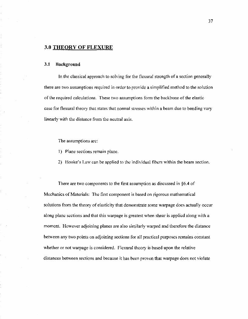
There are two components to the first assumption as discussed in §6.4 of
Mechanics of Materials: The first component is based on rigorous mathematical
solutions from the theory of elasticity that demonstrate some warpage does actually occur
along plane sections and that this warpage is greatest when shear is applied along with a
moment. However adjoining planes are also similarly warped and therefore the distance
between any two points on adjoining sections for all practical purposes remains constant
whether or not warpage is considered. Flexural theory is based upon the relative
distances between sections and because it has been proven that warpage does not violate

38
this relationship between plane sections and the assumption that plane sections remain
plane remains valid.
The second part of this assumption is that when a beam is subjected to pure
bending the positive strains on the outermost tensile surface are accompanied by negative
transverse strains, this curvature is classified as anticlastic curvature. Likewise the
negative strains along the outermost compressive surface are accompanied by positive
transverse strains; this type of curvature is classified as anti-synclastic curvature. See
Figure 3-1. The classical approach to solutions of reinforced concrete sections ignore this
behavior.
Remain Straight
Figure 3-1 Beam in flexure with saddling effect
39
The second assumption, based on Hooke's law, Equation 3-1, states that
individual fiber strains can be used to calculate individual fiber stresses and visa-versa.
e = - (3-1) E
Where the variables are defined as follows:
s = strain
E = modulus of elasticity of the material, commonly referred to as
Young's Modulus
a= stress
3.2 Theory of Flexure in Shallow Reinforced Concrete Sections
In the study of reinforced concrete additional assumptions are made in series with
the first two presented; assumptions 4, 6 and 7 are generally attributed to Charles S.
Whitney but they were obtained from "Design of Reinforced Concrete ACI 318-08 Code
Edition" for this thesis.
3) The strain in the reinforcing steel is the same as the surrounding concrete prior
to cracking of the concrete or yielding of the steel - this is a continuation of
the second assumption
4) The tensile strength of concrete is negligible and assumed to be zero
5) The stress-strain curve of the steel is elastically perfectly plastic
6) The total force in the compression zone can be approximated by a uniform
stress block with magnitude equivalent to 0.85/'c multiplied by a depth of a
7) The maximum allowable strain of concrete is 0.003
40
The general arguments that form the basis of Hooke's Law remain as valid for
reinforced concrete sections as they do for isotropic homogenous material sections when
subjected to small strains.
In general the tensile strength of concrete is around 10% of the compressive
strength. When loaded the tension zone of a concrete section will begin to crack under
very light loads destroying the continuity of the section and any tensile reinforcement
will be forced to carry the tensile load in its entirety.
The assumption that the stress-strain curve of steel is elastically perfectly plastic
implies that the ultimate strength of steel is equivalent to its yield strength. In effect, this
results in an underestimation of the overall ultimate strength of a given section due to the
reinforcing steel but it produces a more predictable mode of member failure.
The stress distribution in the compressive region does not maintain a linear
relationship with respect to distance from the neutral axis due to the nature of the
constituent materials used to manufacture concrete. Rather the stress distribution is in the
form of a parabola as shown in Figure 3-2 c.
Whitney developed an equivalent rectangular stress block that provides results of
equal accuracy for the compressive strength of a concrete section that avoids the rigorous
mathematical calculations required to compute the area of a parabola. This block has
41
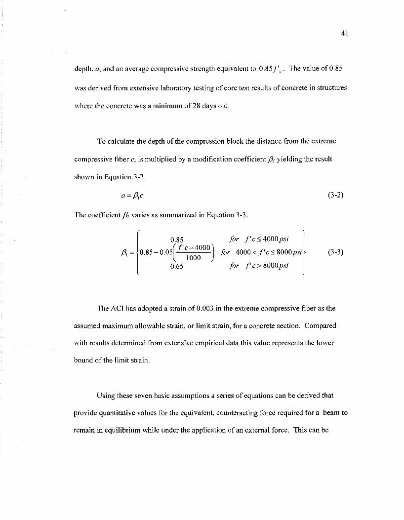
depth, a, and an average compressive strength equivalent to 0.85/'c. The value of 0.85
was derived from extensive laboratory testing of core test results of concrete in structures
where the concrete was a minimum of 28 days old.
To calculate the depth of the compression block the distance from the extreme
compressive fiber c, is multiplied by a modification coefficient Pi yielding the result
shown in Equation 3-2.
a = pxc (3-2)
The coefficient /?/ varies as summarized in Equation 3-3.
A 0.85-0.05
0.85 far f'c<4000psi
/ ' c - 4 0 0 0 j 4000 < / ' c < 8000 mz 1000 J
0.65 for fc> &000psi
(3-3)
The ACI has adopted a strain of 0.003 in the extreme compressive fiber as the
assumed maximum allowable strain, or limit strain, for a concrete section. Compared
with results determined from extensive empirical data this value represents the lower
bound of the limit strain.
Using these seven basic assumptions a series of equations can be derived that
provide quantitative values for the equivalent, counteracting force required for a beam to
remain in equilibrium while under the application of an external force. This can be

42
explained by visualizing the two forces as vectors, equal in magnitude and opposite in
direction, acting at any two locations along the centerline of the cross section. Summing
the forces in the axial direction T = C, i.e. the tensile forces provided by the
reinforcement present in a section are opposite and equal to the sum of the compressive
force provided by the concrete; reference Equations 3-4 through 3-8.
T = A,fy (3-4)
where
C = 0.85/'c/?,c6
a = (5xc
:.c-al[5x
T = C=zAtfy=0.Z5fcab
(3-5)
(3-6)
(3-7)
(3-8)
o
•C=0.85fcab a-PlC
T=Afy
(a) (b) (c) (d)
Figure 3-2 Graphic representation of forces within a reinforced concrete section

43
Variables are defined as:
a = effective depth of the compressive block
As = area of non-prestressed steel
fy = yield strength of non-prestressed steel
f'c = compressive strength of the concrete
b = the width of the section
c = distance from extreme compressive fiber to neutral axis
Using the relationships show in Equations 3-4 through 3-8 and solving for a
yields the result shown in Equation 3-9.
A f a = '-^— (3-9)
0.85 fcb
Solving for the internal resisting couple between the tensile and compressive
forces yields the nominal strength or moment resistance of the section M„, shown in
Equation 3-10.
Mn -AJ^d-^j = 0.85/>Z>(V£) (3-10)
3.3 Theory of Flexure in Deep Beams
Deep beams are a common structural member for which an accurate solution
cannot be reached using the aforementioned techniques. Deep beams are structural
members defined by the relationship between beam width bw, beam depth h and clear

44
span /„. Per ACI 318-08 §10.7.1, deep beams are members loaded on one face and
supported on the opposite face so that compression struts can develop between the loads
and the supports and have either:
a) clear spans /„, equal to or less than four time the overall member depth; or,
b) regions with concentrated loads within twice the member depth from the face
of the support
Deep beams or deep beam regions begin to show crack propagation at loads in the
range of xhPu to xliPu, where Pu represents the concentrated load, and plane sections are
no longer assumed to remain plane. This invalidates the first and most fundamental
assumption discussed in this paper for the solution of reinforced sections. Therefore
other more advanced methods must be employed. One of these is the method of Strut-
and-Tie Model (STM) an inherently conservative method for solving the forces within
these member's sections. The overarching motivation of STM is weighted toward
conservatism in the solutions it provides and to transfer as much of the applied loading as
possible into compression using the fewest number of members.
The foundations of STM are attributed to the truss method work done by Ritter in
1899 developed as a means to explain the dowel action of stirrup reinforcement.
However it was not until the 1980s that the truss method transformed into STM and was
used to find solutions for the discontinuous regions within deep beams.

The method of strut and tie models is not exclusively limited to deep beams, it
also has valid applications in corbels, dapped-end beams and the discontinuous regions,
or D-regions, within shear spans. Mathematically a D-region is defined as a region
located within a distance equal to the member depth h, from the beam/support interface
or a region located a distance h from each side of a concentrated load; reference Figure 3-
3 for examples.
•KH 4)1*, h, h.
h h
(HE Ay?
\>>t
'TO -4 ~A~
JJ ttmmtmt
(a) Geometric discontinuities
O
(tf
1)1'
lt)l" 2h
fW Loading and geometric discontinuities
Figure 3-3 ACI318-08 Fig. RA.1.1 (a and b) - D-regions and discontinuities (Reprinted with permission from the American Concrete Institute)
A D-region within a beam is defined as an inter-beam span where traditional
moment and shear strength theory no longer applies as based on the assumption that
plane sections remain plane, and loads are not reacted by beam action but rather they are
reacted primarily by arch action, as such these D-regions can be isolated and viewed as a

46
deep beam. In these regions the ratio of shear deformations to flexural deformations can
no longer be considered negligible.
At its core STM disregards kinematic restraints, only gives an estimation of
member strength, and it conforms to the lower boundary of theory of plasticity, i.e. only
equilibrium and yield conditions need be satisfied. The solutions for the capacity of
members found using the application of this lower bound theory are estimates that will
provide member capacities which will be less than or equal to the load required to fail the
member; thus the inherently conservative nature of STM solutions.
The two greatest similarities between the ACI 318-08 and AASHTO LRFD code
provisions are the basic set up of the solution, and how the truss members are chosen.
After the global forces have been determined for a particular member, a truss model is
chosen to represent the flow of forces within that member. The goal for development of
any truss model is to use the lowest number of members required to satisfy equilibrium
and safely transmit the forces into the supports. After a truss model has been developed
the forces within that truss are analyzed by using the method of joints, the method of
sections, a combination of both or using a CAD program.
Members in compression are designated struts and members in tension are
designated ties. The intersection of any two or more members is designated a node, as
shown in Figure 3-4.

47
T-c,r—
(a) CCC Node (bJCCTNode
Figure 3-4 ACI318-08 Fig. RA.1.5 (a and b) - Hydrostatic nodes (Reprinted with permission from the American Concrete Institute)
There are few similarities that exist between the ACI 318-08 and AASHTO
LRFD codes with respect to STM efficiency factors. The basic premise for the
implementation of the method using either code is the same but the way that these forces
are resolved within the individual strut and nodal members is the area of greatest
divergence between the two codes. § 4.2 provides a comprehensive explanation of the
differences in the STM between the ACI 318-08 and the AASHTO LRFD 2nd Ed. and §
5.2 discusses the differences in the results obtained from each code.

48
4.0 ANALYTICAL PROCEDURE
4.1 Shallow Beams
In order to simplify the programming phase of the project, an analytical approach
was used rather than a design approach. Doing so reduced the required number of IF
logic statements, shortened the overall length of the EXCEL program, simplified the
program used and focused the project on the analysis of results rather than programming.
All spreadsheets used in the shallow beam analysis were vetted via direct comparison
against example problems 7.4 and 7.5 from the Notes on ACI 318-08 Building code
Requirements for Structural Concrete. Results from the spreadsheets matched those in
the example problems exactly.
Each series of analytical calculations were performed using sections having
similar geometric and identical material properties. The yield strength of the reinforcing
steely, was set at 60ksi and the crushing strength of the concrete f'C) was set at 4ksi. Ten
different geometries were analyzed in a series of four different calculations with each
calculation using three different values for the following variables; flange width b, web
width bw, flange depth tf, and the depth of reinforcement d. Ten arbitrary sections with
the following geometries, graphically described in Figure 4-1, were chosen for analysis.

49
tf
ik
-» b
d
1 bw — * •
-fig w
• » •
* i
f h
"!
Figure 4-1 Section geometry
The values used for each variable's analytical case are listed below in Table 4-1.
Table 4-1 Values for variable and fixed geometry for each case
VARIABLE VALUES
b
bw
d
tf
36in. 42in. 54in. 14in. 18in. 21 in. 24in. 30in. 36in. 2in. 6in. 10in.
FIXED GEOMETRY
tf
bw
d b tf d b bw
tf
b bw
d
4in. 14in. 24in. 36in. 4in. 24in. 36in. 14in. 4in. 36in. 14in. 24in.
For each case the assumed area of provided reinforcing steel was varied from zero
to an arbitrary value of 20 square inches. This was accomplished in incremental steps of
0.50 square inches. However only data within and inclusive of the boundaries
determined by Asmi„ and Asmax would be considered for final analysis.

50
Because each code specifies a unique analytical procedure, the focal crux of this
paper, separate programming approaches were required for both the ACI 318-08 and the
AASHTO LRFD in order to reach solutions. Each procedure is described in detail in the
following sections.
4.1.1 Stress Block Depth Factor fit
The sole quantity that was independent of the code provision used and could be
calculated simultaneously was the stress block depth factor, /?/. Used in computation of
the location of the neutral axis the method for computing the value of /?/, is identical for
both ACI 318-08 and AASHTO LRFD codes and was computed using a simple nested IF
statement as described in Figure 4-2 below.
5 fc < 4.0fc/ Yes Pl = 0.85
No
4.0 < f\ < 8Msi Yes A=0.85-(0.05*(/ 'c-4))
No
f\ > 8.0*5/ > Y e s » px = 0.65
Figure 4-2 IF logic statement for computation of stress block depth factor /?/

51
4.1.2 ACI318-08
4.1.2.1 Limits of Reinforcement
As defined by ACI 318-08 the minimum area of reinforcement Asmin, is the
maximum value of the following two equations; both of which are functions of section
geometry, the yield strength of reinforcement and the crushing strength of concrete.
A, . = Maximum] s mm
3V/'C1000
V ->y Aiooo Kd
(( 200 v/,1000
hd j
(4-2)
ACI 318-08 defines the maximum area of reinforcement Asmax, as a fraction of the
balanced area of steel for a section.
A, =0.63375 A . . smax. sbal
(4-3)
Where the balanced area of reinforcement ASM, is computed as shown in Equation 4-4.
Asbai is also a function of section geometry, yield strength of reinforcement fy, stress block
depth factor ft, and the crushing strength of concrete f'c.
4„=0.85 i f , \ J y J
( (6 -0 /+0 .375 A M ) (4-4)

52
4.1.2.2 Location of Neutral Axis c and Depth of Compressive Block a
The ACI 318-08 utilizes a variable called the reinforcement index zu, based on the
ratio of reinforcement and computed as shown in Equation 4-5.
A f f m = - ^ = p^>- (4-5)
bdfc Ffc
crwas used to evaluate the preliminary value for the depth of the compressive section,
denoted in this paper as a' for clarity, as shown in Equation 4-6.
a'=1.18fflr/ (4-6)
This preliminary value a' was used in the calculation of the preliminary depth of
the neutral axis which has been denoted in this paper for clarity as c' shown in Equation
4-7.
a' c'=— (4-7)
A
Both of these preliminary values were used only for the evaluation of section
behavior via comparison to the flange depth tf, i.e. the determination as to whether the
section was in rectangular action or flanged action and therefore if the web carried any
compressive load.
These preliminary results for a' and c' determined the method used to calculate
the working value for the depth of the compressive section a, and the working value for

53
the depth of the neutral axis c, by means of IF logic statements. The grayed out cells on
the left hand side of the flow chart in Figure 4-6 offers a comprehensive view of this
procedure.
After a value for the depth of the compressive section a, had been obtained and
the depth of the neutral axis c, had been established, an IF statement was used to
determine whether the section behaved under T-section or rectangular action, i.e. if the
depth of the compressive section was greater than or equal to the flange depth a < t/. This
in turn provided the appropriate formula to solve for the factored moment capacity for the
section. See Figure 4-6.

54
4.1.2.3 Strength Reduction Factor (j>
The depth of the neutral axis was also used in the determination of the strength
reduction factor <f> based on ACI 318-08 reproduced below in Figure 4-3.
<p = 0.7 + (£, - 0.002) (2QQ
0.90
0.70 0.65 Other
Compression! controlled
<p = 0.65 + (£,- 0.002) (22S)
Transition Tension controlled
e, = 0.002
§ = 0.600
€, = 0.005
i = 0.375
Figure 4-3 ACI 318-08 Fig. R9.3.2 - Strength reduction factor (Reprinted with permission from the American Concrete Institute)
Another nested IF statement was used within the Excel program to determine this
value as shown in Figure 4-4.
The moment capacity could then be computed using the given values for A ,
section geometry, fy,fc, and the calculated values for c, /?/, and if required the web and
flange moment capacities, Mnl and Mn2 respectively. A sample Excel worksheet is shown
in Figure 4-5.

55
Figure 4-6 shows the preliminary calculations which were contained in hidden
cells, these cells are represented by lightly shaded columns. This procedure is illustrated
by the flowchart in Figure 4-7.
Figure 4-4 ACI318-08 calculation of strength reduction factor ^

3 oro"
B
"1
ffi
4-5 «3
65 3 •a
* o « *—
t»
•o readsh » « t analy: 33"
* 3 01
X p^
s
12486
go
o
_1
_»
.
©
b en
o
o>
o
*?5
Bo
o B
ib
g&S
lil —
*•
H-
vJ
gte-
f
-J
-4
b»
en
Ol
00
o o
go
BB
b H
~>
m
i to
m
©
o (O
C
O
o o
o o
12034 CO
o I.500 00 L».
-s
|
O)
O)
CO
en
o o C
O
-fc.
-*•
o CO
o o
1566 '->.
o OOOl
-vl
4*.
CO
en
en
00 .^
CD
O
GO
—
A.
O o CO
o o
0801
Ko
CO
en
o o en
b CO
co
en
b 00
CO
o k>
-4
CO
o CO
o o
10577 CO
CO
b o o en
CO
en
N
J en
b en
CO
o Ko
4*
oo
o CO
o o
m
s>
Wsl
'
A
L
10057 o> ^
r^
fcrr
. ..
*•£"
y*
*>¥
P°
^SB
* us
jSlte
c>
sip
^ i,
^ r CJ
l JlM
N
>1
&
_».
wB
k C
D 4
s@pV
-jT
fj
*y
^ ii •">
• ^
F
|\2
W$t
$ 10
flfif
'*'
"•-
o ©
-»•
S
"«J
0»
o e
co *
£ o
©
o ©
CO
en
o b 0
0 b o o *.
b —i.
4*.
CO
b N)
N3
O
CO
N
>
O b o o
00
CO
-
J en
en
-j en
o o 4*.
CO
N
J en
CO
b -vi
en
p 00 o o b o o
00
j>.
eo
en
-j b o o -N
b eo
-N
|
eo
4*.
eo
-*
p O)
00 o b o o
o V u
-S*
00 w
Ol
JO
o>
9*
<0 w
o>
4*.
© o o «* *.
o o p o>
«*
© <o
o o
-vj
00
C7>
4*
. bo
en
en
o o eo
^ 4*.
eo
eo
1*.
00
O)
p en
CD
o b o o
-vl
N)
CO
C
O
en
en
b o o eo
4*.
O)
o K>
b 4*.
-*
p 4*.
-&.
O b o o
en
-4
b pi
en
o o CO
-4
N3
NJ b CO
en
p eo
M o b o o
en
—i. 4*.
-*
en
b o o NJ b 00
ji.
N>
Ji". en
-*
p N>
O
O b o o
en
en
en
b 4*.
en
o o ro
en
CO
en
Ni
Ko
o en
p o 00 o b o o
4*.
CO
--
j
Ko
JV
b o o NJ
CO
o -v
l
-i
.
b en
-*
o b CO
en
o b o o
4*.
eo
CO
b eo
en
o o N>
b —X
0
0 _>.
^ __i, en
o b 00 4*.
o b o o
eo
-N
|
en
00 b eo
b o o _x
^v
l
eo
o _».
ji.
->i
-*
o b •vi
Ni
o b o o
to
—X
en
-vl
b N)
en
o o _&.
Ji.
4*.
N>
_x k>
IO
en
o b en
o o b o o
N>
en
C
O
CO
-
»•
N3 b O
O k
Li. en
eo
o b 00 o o b 4*.
00 o b o o
"
J»
a- §sr
_x
^?~*
»
CO
%
^^
£p
KJ
>»
. ; *~
-
jji
; .-
: _»
. .'
a*:
on ^
Sl
eo S
^^
•^
^f
o p
03
0>
en
-*
en
w
—
Ki'
t
o^
kj
j®fe
eo
iH
H
01
^^
sr>l
O
|f
ti
o ^
§*
eo
^@
^^
P f^
'* *
°fes
b ^f
t ^^
p^^
o
^p
^.
o
_A
w
00
N3
CO
_!.
b o o o en
-v|
-j o 4>.
CO
o o b N
) 4^
o b o o
644.7 o en
o o o Ko
00
00 o Ko
4
. en
o b —X
NJ
O b o o
0.0 o b o o o b o o o b o o o b o o o b o o
5
^ °
5*
3 3
>
(/)
o S) £>_
a «- Bendi 3 E
Q
> o •"
•"
CO
00 1 o en
as

lO
o 1 0
0
co ^ o
<
o (S
3
(M
C
S c
S
<
o o o o o o o d o o o d o •<*
CM
00
in
to
o oo d 0
0
~ t
h-
00
O)
•^
a> 0
0
CM
d CO
•sr C
M
d o>
o o d o •*
CM
0
0
lO
CO
,-00
t^
CM
•
^"
CO
r--00
O)
•*-'
00
f-
in
d CM
o>
d N-—
o d o •sl-C
M
00
in
CO
1^. t—
C
M
00
CO
in
1
N-
00
o>
•ST m
*> fw
b °^
^S—
jSjg oo
^M
^ 0
0
lis H
J|C
O
*Ss|i; C
M
sill ^ p
g^
'-'i-i^
$©
&
O
•T
»
^*
4m c4
-'JflKs C
O
^U&
j' L
O
55*° t*J^ oo |jg
p cd ;ijgO
^" ^
:j3BB^^ 0
5
3fT
- ' r~ rljlh
t h~
"«
8g
C0
WO
>
W;-"*
' 'JE?
M
r*-in
T
—
V"
OO
0
0
d in
0
0
o d o T
CM
C
O
in
co
CO
C
O
CM
•
""
CM
N-
00
CO
•s
f
CO
•
<*
•
•^
T~
CO
C
M
CM
CO
M
" O
d o
•sr C
M
oo lO
C
O
00
00
CO
0
0
^1" 0
0
1
r*~
00
CO
•
^
m
CO
N
; T
_
w
r-CM
in
o d o •
*
CM
0
0
m
CO
m
T™
CO
N
-h
-<M
h-
00
O)
•*•'
W
CM
O
C
M
T-
CM
1
^
,_ C
O
o d o *•
CM
0
0
lO
CD
OO
C
M
Tf
co o CM i
h-
00
o>
•tf
•* C
O
CM"
1^-
co °> O
) C
D
O
d o •*
•
CM
0
0
in
CO
CO
f>
C
M
CO
C
O
1
r
00
G)
•<r
CO
o CO
CM*
CO
^ CM
CM
00
f^.
O
d o •"
*
CM
oo to
C
O
o>
ID
00
to
CD
t
N-
00
o>
•*
CM
o>
OO
C
M
00
LO
CM
h-
00
o d o •<r
CM
C
O
m
co
CM
C
M
CO
T
~*
P--
oo o>
•*r ,_
00
T—
co"
s t--
CM
in
o>
o d o •sf
CM
0
0
m
CO
89Z69 N-
CO
o>
•Si"
T—
N-
M"
CO
O
in
o>
CM
•sr
o
T—
d o •<a-C
M
00
in
CO
a> t*-
ai C
O
CO
N-
00
at
•<r
o <o h
-
co"
CO
o>
CO
CO
T
—
T—
d o •r
CM"
oo m
co
•*
•
in
•^
;
CO
o CM
N-
00
CO
<*"
CM
«
"•
o * <? T
"
s ^-
o o *t
c<i C
O
to
to
T-
o» C
O
o to
CM
Is.
OO
C
O
"*
•s-
It A
u
CO
"* o •
*'
CM
CO
CM
C
M
T—
d o T
CM" oo in
C
O
m
o>
^ o>
CO
C
M
N-
00
O)
•*
"
OO
o
CO
"*'
oo 0
0
CO
CO
o CO
T
—
d o •*
CM
0
0
m
CO
o>
o>
T—
•St
CO
C
O
1^.
oo o>
•
r
N.
CM
C
O
•^:
CO
C
O
CO
CO
CO
C
O
T-
d o •<*
CM
oo in
C
O
o>
CO
•
f C
O
O)
CO
h-
00
o>
-*' #•
-.tvo
>
,*f-
•"* f
'
•"«S
B"O
>
E?
.l^
3"
> .:
*f
00
'*^
r •T
W
t-
•<S
*-0
O'
O
ftt C
M
m- oo
*» ">
«e>. co
O.
CO
C
O
"^
0
O
CM
m
o»
v m
<
* -51-
l*- r^
. to
oo
A-
O
•*
-r
*s-R
A
to
o <M
in
"
m
CM
CO
in
x—
O
o •^
•
c\i 0
0
in
CO
CM
T
—
d r-T~
m
i^-
00
a> •<
t m
CO
•
*
in*
T—
t^
C
O
•*
"
m
CO
T
-
o
o
•sr C
M
oo in
C
O
o O)
oo" C
M
r--m
h-
00
CO
•sT
•f
oo t^
-
iri
r
T™
CO
M1
•^J" N
-T
~
o o •"
*•
CM
0
0
in
CO
r
r-ca co C
M
<6
N-
co o>
^'
•sf N
-O
C
D
CO
C
D
to"
CM
0
0
T—
o o ,^-C
M
oo m
C
D
-f
N-
CO
oo r«-co
r-00
o>
•^
CO
C
O
CO
to
00
o in"
T—
CO
T
—
o o •<t
CM
0
0
in
to
o oo ,_' a> C
M
i-^
N-
00
O)
•*
IO
o>
CO
to
im
siM
H
m
Hi
CM
o>
T-
O
IM
9 9 ^n ii^
jMS
iifeif
CM
lf>
to
^,
CO
IX
.
W
||Sn
iS
'M X
(0 E
z
a
00
o
00
ro
u c
r V
V
J3
t» •O
OS
I. a. 13 w
V
J* "a. S
3
&0

58
Given b,bw,d,tf,f'c,fyand As
' * ^ - • * * •
fcftSI
&:*
•W».',ttfoji'iAKJ
1 Is ^ < a' .Yes.
,No
o = -(4/,)
<0.S5feb)
c = -a
Is a>t Yes
0«pdi««
^*Mmm i-iSA-'^Jj^A^ffl
^^^MS'i •i.%Mtaa.inittri
Is ^ < c' Yes tf = ((4-A/)/,) (0.85/ 'e6J
No
/ M„=^(M„1+M„2)
•No
M . = ^ / , | r f - -a
Figure 4-7 ACI318-08 excel program logic flowchart

59
4.1.3 AASHTO LRFD
4.1.3.1 Limits of Reinforcement
The procedure for determining Asmin as specified by AASHTO LRFD Equation
5.7.3.3.2-1 did not require the use of any IF logic statements and was determined as
shown in Equation 4-8.
A, . = 0.7bd s mm w f ,
(4-8)
However, determination of the AASHTO LRFD value for Asmax did require an IF
statement that was dependent on the value calculated for the maximum depth of neutral
axis c. AASHTO LRFD § 5.7.3.3.1 defines the limitation for maximum reinforcement as
follows:
5.7.3.3.1 Maximum Reinforcement The maximum amount of prestressed and nonprestressed reinforcement shall be such that:
c
in which:
<0.42 (5.7.3.3.1-1) d„
A fd +A f d d^=_sJ_y^ PsJps P (5.7.3.3.1-2)
Afy + dps fpi sJ y psJ ps
where: c = the distance from the extreme compressive fiber to the neutral axis (in.)
de = the corresponding effective depth from the extreme compressive fiber to the centroid of the tensile force in the tensile reinforcement (in.)
If Equation 1 is not satisfied the section shall be considered to be overreinforced.

60
The final statement leads to the conclusion that is summed up mathematically in
Equation 4-9, also reference Figure 4-9.
c — > 0.42 -> Overreinforced (4-9) d
Setting AASHTO LRFD Equation 5.7.3.3.1-1 equivalent to Equation 4-9 and
using the known depth for the centroid of reinforcement the maximum value for the depth
of the neutral axis for a section while remaining underreinforced can be found simply, as
shown in Equation 4-10. For clarity within this paper this preliminary value for c will be
denoted maxc.
maxc = 0.42(i (4-10)
Using one of the two approaches described in detail in §4.1.3.2 and solving for c
one can readily determine the limiting area of reinforcement allowed.
4.1.3.2 Location of Neutral Axis c, and Depth of Compressive Block a
The AASHTO LRFD code provides two methods of determining the depth of the
neutral axis; the conservative approach and the refined approach.

61
When using the refined approach the method used to determine the depth of the
neutral axis is based on the action experienced by the section, i.e. whether or not the
beam is under rectangular action or T-section action.
If the beam is under T-section action then c is computed as shown in Equation 4-
11.
AJy-As\fy\-0.S5f'cft(b-bw)hf
c = l-n (4-11) 0.85 /cM,
Otherwise c is computed by the method described as the conservative approach
which is identical to the method used by ACI 318-08, reference Equation 4-12. The gray
box in Figure 4-11 highlights this process within the overall AASHTO LRFD analytical
procedure.
c=Afy-A\fy\
All AASHTO LRFD analysis performed and discussed in this paper utilized the
refined approach during the calculation of the depth of the neutral axis and an EXCEL IF
statement was programmed using the value for maxc from Equation 4-10 as shown in
Figure 4-8.

62
Yes Is maxc>tf } p. 4max=maxc0.85/'c/?,£>„ +
0.85fcj3l(b-bjtf
fy
Figure 4-8 Determination of AASHTO LRFD.4,
4.1.3.3 Strength Reduction Factor ^
The strength reduction factor </), as defined by AASHTO LRFD also uses the limit
of Asmax to determine its value. If the area of reinforcement is less than Asmax then ^ = 0.9,
otherwise ^ = 0.7. See Figure 4-9.

63
0.005 0.002 1 1 ste
1 1 # Factor < ^ for bending I J » <* for compression
ACI318-05 Minimum Transition I (c/djmi„ 0.375 0.60 1 - ' — J *r. i Tension controlled t Transition • Compression controlled ue
\ (under-reinforced) | f " *f (over-reinforced)
A . „ ,„ Minimum 0.42 AASHTO I I ^i£_
L R F D i-- Under-reinforced j ^ , - „nmMmaBiMS /„„ tm,BuinT,\ * - * j — * • f for compression (no transition)
(f> for bending I i j—+• Over-reinforced
Figure 4-9 AASHTO LRFD and ACI 318-08 limits of reinforcement
The AASHTO LRFD moment capacity was computed using the identical values forAs,
section geometry, reinforcement yield strength^, and concrete crushing strength/ 'c , as
for the ACI 318-08 test cases along with the AASHTO LRFD specific calculated values
for depth of neutral axis c, and strength reduction factor 0. A sample EXCEL worksheet
is shown in Figure 4-10 and Figure 4-11 illustrates this procedure by means of a
flowchart.

64
* &*«m !
c>=t,
fc a > a t f •
Moment k*in.
0.0 644.7
^hflSBiSc.'; 1282.8 1914.2 2539.1 3157.3 3768.9 4373.9 4972.2 5564.0 6149.1 6727.6 7299.5 7864.8 8283.7 8354.7
- ^ w l f l 8900.2 9428.7 9940.2 10434.7 10912.1 11372.5 11816.0 12242.4
Mi
As 0.000 0.500
:14M: i 1.000 1.500 2.000 2.500 3.000 3.500 4.000 4.500 5.000 5.500 6.000 6.500 6.936 7.000
* JMPMr'-i 7.500 8.000 8.500 9.000 9.500 10.000 10.500 11.000 11.036
AASHTO - LRFD C
kip 0.0
30.0
60.0 90.0 120.0 150.0 180.0 210.0 240.0 270.0 300.0 330.0 360.0 390.0 416.2 420.0
*• ••MMSht'-450.0 480.0 510.0 540.0 570.0 600.0 630.0 660.0
c 0.000 0.288
a 0.000 0.245
c/de
0.000 0.012
4>, Bending 0.9 0.9
{. filly l JflHB b jHH^S^H^i 0.577 0.865 1.153 1.442 1.730 2.018 2.307 2.595 2.884 3.172 3.460 3.749 4.000 4.095
""i'^roWksa 4.836 5.578 6.319 7.061 7.802 8.544 9.285 10.027 10.080
0.490 0.735 0.980 1.225 1.471 1.716 1.961 2.206 2.451 2.696 2.941 3.186 3.400 3.481
• 'lfflWHIrvi 4.111 4.741 5.371 6.002 6.632 7.262 7.892 8.523 a.568
0.024 0.036 0.048 0.060 0.072 0.084 0.096 0.108 0.120 0.132 0.144 0.156 0.167 0.171
•««3^Wtes 0.202 0.232 0.263 0.294 0.325 0.356 0.387 0.418 0.420
0.9 0.9 0.9 0.9 0.9 0.9 0.9 0.9 0.9 0.9 0.9 0.9
0.9 0.9
£;4feUws 0.9 0.9 0.9 0.9 0.9 0.9 0.9 0.9 0.0
Figure 4-10 Sample excel spreadsheet for AASHTO LRFD analysis

65
Given b,bw,d,tf,fc,fvm& As
Is tf> AA sJ y
0.85/'cfl&J (0.S5 feftbw)
No
c = -(4/,-0.85/'cfl(ft-ft i r)f /)
(0.85/VA^)
a = /^c
J
Is c<^ Yes
/ Mu=tAsffy\d--} a
No
Mu =Msffy(d~yO.S5PJ'c(b-bw)tJ v a- —
Figure 4-11 AASHTO LRFD flowchart

66
4.2 STM
4.2.1 Introduction
Each series of deep beams was analyzed using the STM method as described by
both the ACI 318-08 and AASHTO LRFD 2nd Ed. code provisions. Results were then
compared to the work performed by Ha on identical sections and compared as a
percentage of the maximum allowable load to the test load.
The solutions for this series of beams were worked in three phases; first a
graphical STM solution was solved to determine the maximum allowable strut and tie
member sizes, then the truss geometries from the first step were solved for using a unit
load and classical hand calculations; finally an EXCEL spreadsheet created specifically
to solve for the STM model element capacities (struts and ties) based on the previously
defined geometry from step 1 was utilized. This spreadsheet then converted the unit load
into an equivalently proportioned maximum allowable service load which led to the final
solution to the problem.
Concrete strength was assumed to be 7ksi, the lowest value used by Ha, and
reinforcing steel strength was assumed to be 60ksi. Geometric section properties were
matched to those used by Ha with identical beam sections measuring 44in. x 36in. x 4in.
The location of the openings was specific to each series and constituted the only variable
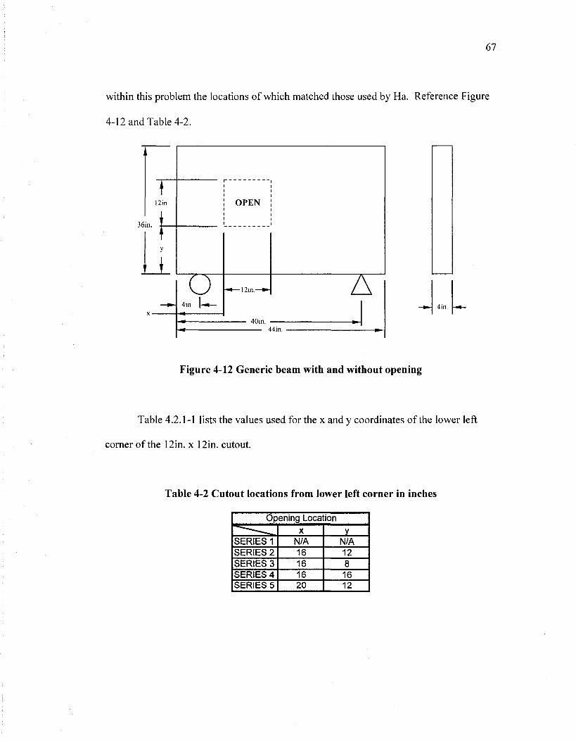
67
within this problem the locations of which matched those used by Ha. Reference Figure
4-12 and Table 4-2.
36in.
12in.
i
TJ 4in.
OPEN
-12in- 7\ 40in.
44in.
4in.
Figure 4-12 Generic beam with and without opening
Table 4.2.1-1 lists the values used for the x and y coordinates of the lower left
corner of the 12in. x 12in. cutout.
Table 4-2 Cutout locations from lower left corner in inches
Opening Location " " • „ ^ _
SERIES 1 SERIES 2 SERIES 3 SERIES 4 SERIES 5
X
N/A 16 16 16 20
y N/A 12 8 16 12

68
The method of STM analysis as employed for purposes of this thesis were for all
intents and purposes identical.
Use was made of Naaman's proposal regarding the compressive strength of
concrete that "...the value oifcu recommended by ACI in Equation (15.7) and Table 15.1
is appropriate enough, given the uncertainty on the evaluation of the state of strain in the
struts."
For completeness Equation 15.7 from the Naaman text reads:
fa, = smaller of 0.85/yc or 0.85/?/'c (4-13)
This upper limit of the effective strength as defined by the AAHTO LRFD of
0.85/yc was used for all AASHTO LRFD based STM calculations performed in this
paper.
This assumptions greatly reduced the complexity of many of the iterative steps
required during the analytical process; when these assumptions were used the method of
STM as described by both ACI 318-08 and AASHTO LRFD 2nd Ed. outside of the values
for strength reduction factors was identical; the strength reduction factors remained
unique to each code.

69
4.2.1.1 Graphical Solution
Pro/E 3-D design software was utilized to provide true scale models and drawings
of each deep beam section to ensure that the largest possible strut and tie members had
been placed in the section. Geometric model constraints were used to ensure that no strut
possessed cross sectional area greater than that of any adjacent node and that all STM
members remained prismatic. See Appendix A - Deep Beam STM Models, Figures A-l
through A-5.
It should be noted that Figures A-2 through A-5 are unstable trusses; that is they
do not satisfy all of the necessary requirements for a stable and determinate structure.
The convention for calculating the determinacy and stability of a structure is shown
below.
r + b = 2n Stable and Determinate (4-14)
r + b > 2n Stable and Indeterminate (4-15)
D -r + b -2n Degree of Indeterminacy (4-16)
r + b<2n Unstable (4-17)
With variables defined as:
r = number of reactions
b = number of beams/truss members
n = number of nodes

70
Using Figure A-2 as an example one can see that the number of members is 9, the
number of reactions is 3 and the number of nodes is 7. Therefore r + b = 3 + 9< 2*7
demonstrating that the structure is unstable. Due to the symmetry of the truss models
unique solutions for each member were possible. A thorough examination of "Examples
for the Design of Structural Concrete with Strut and Tie Models" reveals that many
effective STM models are not considered stable truss structures when evaluated using
Equation 4-17; but they are symmetric trusses and provide satisfactory support because
the members are confined by the surrounding concrete. However, for the asymmetric
truss model shown in Figure B-6 this is not the case and unique solutions for each
member were not found.
4.2.1.2 Hand Calculations
After the truss geometry had been determined as shown in Appendix B - Deep
Beam STM Truss Models Figures B-l through B-5, the individual truss member forces
were solved for using a unit load, basic equations of equilibrium and the method of joints.
Results from these calculations were used as the input into the EXCEL Spreadsheets.
See Appendix C - STM Truss Free Body Diagrams & Solutions Series 1 through Series
5.
4.2.1.3 Excel Spreadsheets
A series of Excel spreadsheets was developed that used concrete strength/'c,
strength reduction factor(s) ^, reinforcement yield strength^, and beam member
71
geometry as inputs to calculate the maximum concentrated load that could be applied.
An iterative process that determined STM applicability was used, i.e. after all maximum
equivalent forces had been determined and converted into a single point load placed at
the midsection of the beam the validity of Vu < </>V„ was checked. If the criteria of Vu <
<f>Vn was met then the magnitude of the maximum point load was considered acceptable.
Spreadsheet logic flow followed the procedure shown in Figure 4-12 and
verification of the strut capacity at midlength and nodal interface was computed using the
code specific relationship details described in Table 4-3.
For all cases documented for this thesis all struts were treated as bottle shaped
with the cross sectional area at strut midlength assumed to be greater than the maximum
area available at the strut-node interface.
Unit load values found during the hand analysis portion were input into the
spreadsheet and the minimum required member width was determined using Pr = 0Pn and
Pn = fcuAcs, where Pr is the calculated force within the strut member, Acs represents the
cross sectional area of the strut and/CM = 0.&5f'cmin(fln,/3s). Since member depth was
held constant at 4.0 inches to remain consistent with Ha's experimental beams the
specific version of the equation used was,
w . = £ (4-18) 4.0/«.0.85/'cmin(/fr,/fo)

72
The minimum required "unit width" calculated from Equation 4-18 was then
divided into the maximum attainable widths as determined using Pro/E to obtain the
percentage increase available. The limiting case was selected and used to calculate the
individual member forces. This value was then used with the previously worked hand
solutions and converted into the maximum applied concentrated load, to be compared
against the test loads used by Ha in his work. These comparisons formed the basis of this
portion of this thesis.
4.2.2 ACI318-08 vs. AASHTO LRFD
As shown in Table 4-3 the effective concrete compressive strength^, is
calculated the same regardless of which code is used; however the member effectiveness
factors and strength reduction factors used by the two codes were very different.
4.2.3 Strength Reduction Factor ^
ACI 318-08 provision used 0.75 for all STM cases whereas the AASHTO LRFD
provided two distinct strength reduction factors based on the member type; <f> = 0.7 for
struts and <j> = 0.9 for ties. Reference Table 4-3 for application.

73
4.2.4 Strut Effectiveness Factors fis
ACI 318-08 contained five distinct strut effectiveness factors J3S, based on strut
geometry, provided strut reinforcement and weight of concrete used. In cases where the
provided strut reinforcement does not meet the requirements of ACI 318-08 section A.3.3
the weight of concrete is used to determine the strut effectiveness factor via the
modification factor X which was related to the unit weight of concrete; X = 1.0 for
normal-weight concrete, X = 0.85 for sand-lightweight concrete and X = 0.75 for all-
lightweight concrete. However for purposes of simplicity the requirements of ACI 318-
08 A.3.3 were always assumed satisfied and therefore fis = 0.75. The AASHTO LRFD
2n Ed. code only provided two strut effectiveness factors based solely on strut geometry,
i.e. if they were prismatic or bottle shaped struts.
4.2.5 Node Effectiveness Factors /&
The number of node effectiveness factors /%, defined by each code was equal at
three; however the two values provided by the AASHTO LRFD 2nd Ed. for C-C-C and C-
C-T nodes were conservative when compared against their counterparts in the ACI 318-
08. See Table 4-3 for exact values.

74
Table 4-3 ACI 318-08/AASHTO LRFD effective strength coefficients
Strength Reduction Factor (p
Strength of Struts
Uniform Cross Section ps
w/Reinforcement Satisfying A.3.3 ps (ACI 318-08 Only)
w/o Reinforcement Satisfying A.3.3 ps (ACI 318-08 Only)
Struts in Tension ps (ACI 318-08 Only)
All other Cases ps (ACI 318-08 only)
Strength of Nodes
C-C-C Nodes pn
C-C-T Nodes pn
C-T-T, T-T-T Nodes Pn
Strength of Ties
ACI 318-08
0.75
f =f A
fcu=0.85psf'c
1.0
0,75 0 60' 0.40
0.60
' n—' cu"n
fcu=0.85psfc
1.0
0.8
0.6 fT=fyAS
AASHTO - LRFD 0.7 Compression
0.9 Tension f =f A ' s ' cu"s
fcu=0.85psf'c
1.0
' ! • ,-.., : - r . ' ' i
' n= 'cu"n
for0.85p.fc
0.85
0.75
0.65 / :
T=fA

75
bVuz<pV„=t(ioJfcbM
Yes
No
Select Strut & Tie Truss Model to Carry Loads/Reactions
Model Truss Member Dimensions Using Maximum Available Area
Solve Truss Model Using Unit Load
Determine Equivalent Maximum Member Forces
Verify Capacity of Struts at Midlength and Nodal
Interface
Detail D-Region Verifying Minimum Reinforcement Requirements have been Met
Figure 4-13 Strut and tie modeling procedure
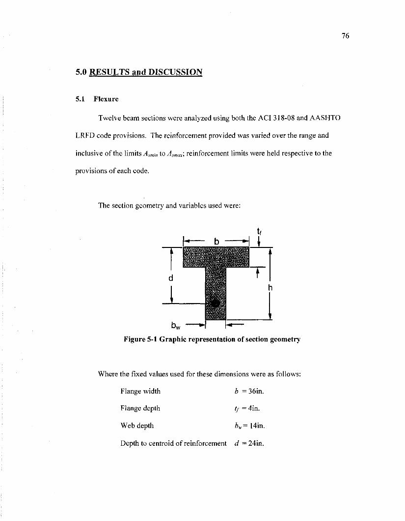
76
5.0 RESULTS and DISCUSSION
5.1 Flexure
Twelve beam sections were analyzed using both the ACI 318-08 and AASHTO
LRFD code provisions. The reinforcement provided was varied over the range and
inclusive of the limits Asmi„ to Asmax; reinforcement limits were held respective to the
provisions of each code.
The section geometry and variables used were:
'W
Figure 5-1 Graphic representation of section geometry
Where the fixed values used for these dimensions were as follows:
Flange width b = 36in.
Flange depth tf = 4in.
Web depth bw= 14in.
Depth to centroid of reinforcement d = 24in.
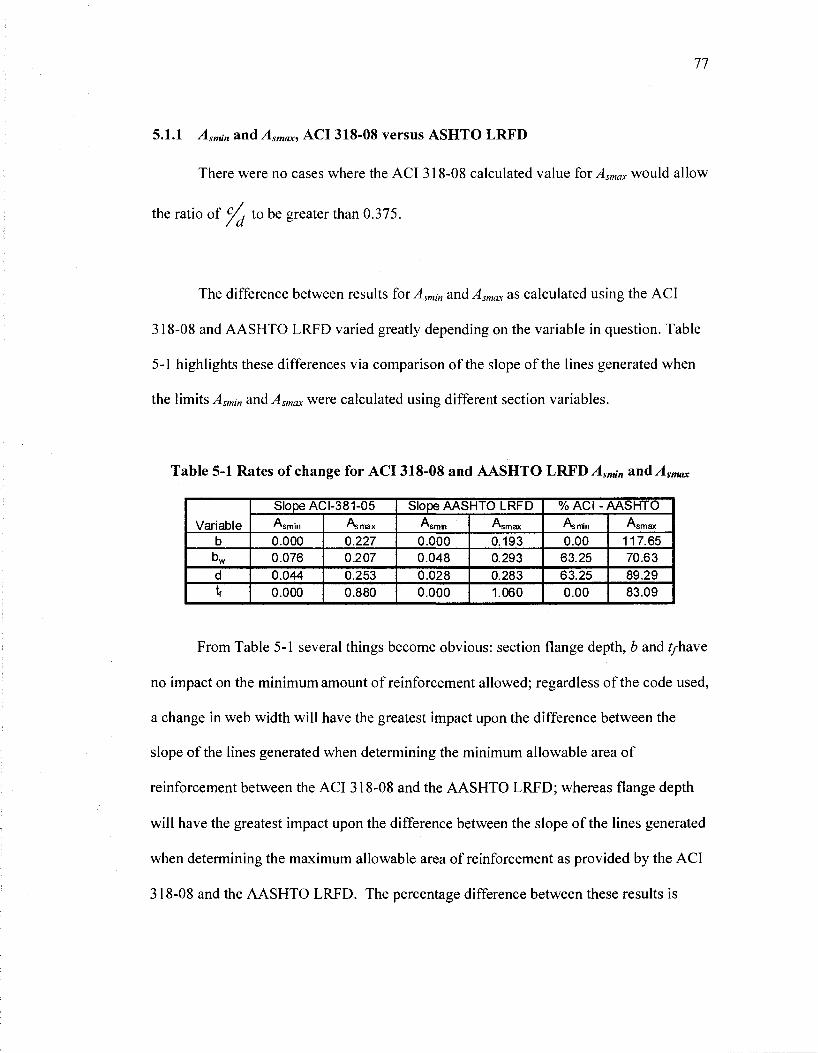
77
5.1.1 Asmin and Asmax, ACI318-08 versus ASHTO LRFD
There were no cases where the ACI 318-08 calculated value forAsmax would allow
the ratio of y, to be greater than 0.375.
The difference between results for Asmin and Asmax as calculated using the ACI
318-08 and AASHTO LRFD varied greatly depending on the variable in question. Table
5-1 highlights these differences via comparison of the slope of the lines generated when
the limits Asmin and Asmax were calculated using different section variables.
Table 5-1 Rates of change for ACI 318-08 and AASHTO LRFD Asmin and A.
Variable b bw
d tf
Slope ACI-381-05 A
0.000 0.076 0.044 0.000
"smax
0.227 0.207 0.253 0.880
Slope AASHTO LRFD A
0.000 0.048 0.028 0.000
A "smax 0.193 0.293 0.283 1.060
% ACI-AASHTO "smin
0.00 63.25 63.25 0.00
"smax
117.65 70.63 89.29 83.09
From Table 5-1 several things become obvious: section flange depth, b and //-have
no impact on the minimum amount of reinforcement allowed; regardless of the code used,
a change in web width will have the greatest impact upon the difference between the
slope of the lines generated when determining the minimum allowable area of
reinforcement between the ACI 318-08 and the AASHTO LRFD; whereas flange depth
will have the greatest impact upon the difference between the slope of the lines generated
when determining the maximum allowable area of reinforcement as provided by the ACI
318-08 and the AASHTO LRFD. The percentage difference between these results is

78
tabulated in the far right columns of Table 5-1. These percentages were calculated by
dividing the values for the slopes of the results found using the ACI 318-08 by the slopes
of the results found using the AASHTO LRFD.
It is of interest to note that the difference between the codes for minimum
reinforcement when based on section flange width and section flange depth, b and tf
respectively, was consistent between the codes while the difference between the codes for
maximum reinforcement was always less when using the ACI 318-08 than the AASHTO
LRFD except when comparing results found using the flange width b as the variable. In
this case the slope of the results found using ACI 318-08 increased by a rate of 17.65%
faster than for those produced when using the AASHTO LRFD provisions.
The slopes of the results found using ACI 318-08 for all other variables were an
average 81% less than the corresponding values calculated using the AASHTO LRFD.
Reference Figures 5-2 through 5-5.

36
38
40
42
44
46
48
Fla
ng
e W
idth
, b
(in
.)
-AC
I31
8-0
8 A
smin
-AA
SH
TO
-LR
FD
Asm
in
-AC
I31
8-0
8 A
sma
x
-•-A
AS
HT
O -
LR
FD
Asm
ax
t 24
in. I
—
b
14
in.
—
*BB
> H
H>
4in
.
,L
f 2
6in
•t
Fig
ure
5-2
A sm
ax
and
Asm
i n a
s a
func
tion
of b

80
c £ < oo
18-0
CO
<
*
c
E <n < Q 14-
. o I CO
s {
X
E < oo
18-0
CO
<
+
X (0 E U) < Q LL 01 _ J
o I CO
s I
4in.
*
i
36in
.-
''
_, r l
26i
i
c _ _ ~ r-
1
«fK>
*o o CM
U4 J2
1 1
o a o
• MM
u a
, 3
,a I
a
s W)
-SO
<b6-4?
('Uj) 'xeuusv ^ ujuisv

16
14
12
c ••=-
10
><
re
E
jj
8 08
c 1 6
v>
<
?—
--
6—1
•—-~
i
. -i
r i-A
o
^
A S
24
26
28
30
3
2
Ste
el D
epth
, d
(in.
)
34
-AC
I 31
8-08
Asm
in
•AA
SH
TO
-LR
FD
Asm
in
•AC
I 318
-08
Asm
ax
-AA
SH
TO
-LR
FD
Asm
ax
14in
36
Fig
ure
5-4
Asm
ax
and
Asm
in a
s a
fun
ctio
n o
f d

18
16
14
~.
12
_c
X g 1
0 < eg
8
c 1 O
ft
<
6
?—
[==t
?—
t=jf ?
— ^
=*
^_
A
5 6
7
Flan
ge D
epth
, t, (
in.)
-AC
I318
-08A
smin
-AA
SH
TO
-LR
FD
Asm
in
•AC
I 318
-08
Asm
ax
-AA
SH
TO
- L
RFD
Asm
ax
36in
.
24in
. 14in
.-
10
tf
zd_L
26in
.
Fig
ure
5-5
4 jm
ax a
nd A
snun
as
a fu
nctio
n of
tf
oo
to

83
5.1.2 As versus Mu
During the determination of the flexural strength of a section based on the area of
reinforcing steel by either ACI 318-08 or AASHTO LRFD code, the difference in
corresponding moment capacity was never greater than 1.4%; the average difference was
0.93%. It was observed that sections analyzed using AASHTO LRFD code consistently
required a larger area of steel to support the same moment than that required for an
otherwise equivalent ACI 318-08 section. All results presented in this section in the form
of tables or percentages represent a ratio between the results found for the ACI 318-08
and AASHTO LRFD code requirements for determining flexural capacity, reference
Equations 5-1 through 5-3.
For all cases analyzed, certain geometric dimensions were found to have greater
influence than others on the amount of reinforcement required to resist a given moment;
results are summarized in Table 5-2 and Figures 5-6 through 5-9.
Table 5-2 Ratio of AASHTO LRFD to ACI 318-08 for M„ per unit ,4,
VARIABLE
b
bw
d
tf
VALUE 36 42 54 14 18 21 24 30 36 2 6 10
ACI 318-05 1189.10 1196.27 1201.20 1189.11 1185.04 1176.01 1189.11 1495.58 1798.78 1197.49 1167.61 1152.80
AASHTO LRFD 1178.79 1186.56 1193.30 1178.79 1171.39 1163.34 1178.79 1481.67 1782.43 1186.04 1164.05 1133.17
% 99.13 99.19 99.34 99.13 98.85 98.92 99.13 99.07 99.09 99.04 99.69 98.30
AAVG
9.31
12.22
13.53
11.54
%AVG
99.22
98.97
99.10
99.01
A MAX
10.31
13.66
16.35
19.63
% MAX
99.34
99.13
99.13
99.69

84
The percentage difference ratio as shown in Table 5-2 is the sum of the applied
factored moments divided by the sum of the areas of reinforcement required for a section
analyzed using the AAASHTO LRFD to carry that moment over the entire viable range
of reinforcement, divided by the area of reinforcement required for the ACI section, i.e.
the range Asmin to Asmax as defined by each code. Equations 5-1 through 5-3 describe the
formulae used in the calculation of this percentage more concisely. This was considered
a convenient method of quantifying the difference in results produced by each code for
the area of reinforcement required to resist an applied moment on a per unit basis, i.e.
applied moment per unit area of reinforcement. The applied moment is a representation
of the applied loads only however it is used in the determination of required
reinforcement during design or analysis of a section via the calculated resistive moment
of the section, M„ = 0MU. Therefore in essence this percentage represents a comparison
between the ACI 318-08 and the AASHTO LRFD of the allowable applied load as
defined by each code for based on each cross section's geometry.
A% = (AASHTO)Mu:As
(ACI)MU:A 100 (5-1)
•* J
where
Asmax
AASHTO- MU:AS=^^- (5-2)
Asmin
and

85
As max
« s As max
IK •smin
is max
1 - 4 ,
v4C/- M • yl = ^sas— (5-3)
/f^min
Examination of the data in Table 1 highlights two consistent traits between the
codes: a) a section designed using the AASHTO LRFD code will always require a larger
area of reinforcing steel than an equivalent section designed using the ACI 318-08 code,
i.e. the AASHTO LRFD will provide a more conservative solution for the resistive
moment per unit of reinforcing steel; b) web width bw, has the greatest effect on the ratio
of steel to flexural strength for any arbitrary T or L flanged section, although this amount
averaged only 1.40% for the section geometries studied.

Resistive Moment, Mu (k*in.) M O O O
-N O O o
CD o o o
00 o o o
o o o o
to o o o
-N o o o
o> o o o
00 o o o
=
• OS
n s
o 1 < 65 »' cr
(D
n> o CO
o b
to b
CO
b
b
b
b
oo b
g
to b E | P |
* •
?
• > > S
HT
<) > W
3 o
CT II
<n •b-
p
a
> o CO
1
00
> V)
X
o
CT
en A. p'
•
> > SH
T
<) > (A
X
o
c-II
en •c
3
O
> o CO
1
co > </> X
o
" cr
-fc. to 3"
•
> >
1HS
() > w
X
o
o-II
<o a> p
>
> O 318
•
00
> (/> X
o —t
cr
CO a> 5 '
HUH > > > > > > > > > o o o m » M j . a a
q q q II n u O O O ui j ^ co a- cr cr * • M <" it II II en * . co i M O)
98

14
00
0 -
0)
-AC
I bw
=14
-AC
I bw
=18
-AC
I bw
=21
-AA
SH
TO
bw=
14
-AA
SH
TO
bw=
18
-AA
SH
TO
bw
=21
AC
I 318
-08
Asm
ax fo
r bw
= 1
4 in
.
AA
SH
TO
Asm
ax fo
r bw
= 1
4 in
.
AC
I 318
-08
Asm
ax fo
r bw
= 1
8 in
.
AA
SH
TO A
smax
for
bw=
18
in.
AC
I 318
-08
Asm
ax fo
r bw
= 2
1 in
.
AA
SH
TO
Asm
ax fo
r bw
= 2
1 in
.
4in.
0.0
1.0
2.0
3.0
4.0
5.0
6.0
7.0
8.0
9.0
10.0
11
.0
12.0
13
.0
14.0
Are
a o
f S
teel
, As
(in
.2 )
Fig
ure
5-7
As
vers
us M
„ f
or v
aria
ble
Z»,

c 3 £ o > (A
1500
0 -
0)
A • O
• • •
-AC
I d=
24in
.
-AC
I d=
30in
.
-AC
I d=
36in
.
-AA
SH
TO
d=2
4in.
-AA
SH
TO
d=3
0in.
-AA
SH
TO
d=3
6in.
AC
I 31
8-08
Asm
ax fo
r d=
24
in.
AA
SH
TO
Asm
ax fo
r d=
24
in.
AC
I 31
8-08
Asm
ax fo
r d=
30
in.
AA
SH
TO
Asm
ax fo
r d=
30
in.
AC
I 31
8-08
Asm
ax fo
r d=
36
in.
AA
SH
TO
Asm
ax fo
r d=
36
in.
4in.
0.0
1.0
2.0
3.0
4.0
5.0
6.0
7.0
8.0
9.0
10.0
11
.0
12.0
13
.0
14.0
15
.0
Are
a o
f S
teel
, As
(in.2)
i d
•*m
—
I 14in
.
36in
.
-®
\ ,i
t 26in
''
Fig
ure
5-8
As v
ersu
s M
„ fo
r va
riab
le d
oo
oo

1000
0 -
80
00
-
6000
- 01
, ' A
• 0 • D •
-AC
I tf=
2
-AC
I tf=
6
-AC
I tf=
10
-AA
SH
TO
tf=
2
-AA
SH
TO
tf=
6
-AA
SH
TO
tf=
10
AC
I 31
8-08
Asm
ax fo
r tf=
2 in
.
AA
SH
TO
Asm
ax fo
r tf=
2 in
.
AC
I 31
8-08
Asm
ax fo
r tf=
6 in
.
AA
SH
TO
Asm
ax fo
r tf=
6 in
.
AC
I 31
8-08
Asm
ax fo
r tf=
10
in.
AA
SH
TO
Asm
ax fo
r tf=
10
in.
24in
.
36in
.
14in
."
T 26
in.
0.0
2.0
4.0
6.0
8.0
10.0
12
.0
Are
a o
f S
teel
, As
(in
.2)
14.0
16
.0
18.0
Fig
ure
5-9
As
vers
us M
u fo
r va
riab
le t
f
00

90
5.1.3 Location of Neutral Axis c, and Depth of Compressive Block a
The depth of the neutral axis has been conventionally defined as described by
Equation 5-4 which is used by both the ACI 318-08 and AASHTO LRFD. This equation
applies regardless of section geometry, that is rectangular or flanged, or whether the
section is in rectangular or T-section behavior when using ACI or AASHTO LRFD
Simplified Conservative Approach.
4Jy-A'sfy
0 . 8 5 / ^ 6 (5-4)
The AASHTO LRFD refined approach, which was the method used for all
AASHTO LRFD based calculations in this paper, differs when sections exhibit flanged
behavior as described earlier in §4.1.3.2. The formulae are repeated below for
convenience.
c=A,fy-A,fy
0.85/'cfl6
c AJy-A\fy-^5fcP,{b-bJhf
0.85/'e/?A,
The results for the depth of the neutral axis using Equation 5-6 were computed for
every 0.250 square inches increase in the area of reinforcement provided; this range was
inclusive of the lower limit of Asmin and the upper limit of Asmax as found by the ACI 318-
08. Because the value for Asmax that was produced by the ACI 318-08 was always less

91
than that found by using the AASHTO LRFD it was used as the limiting value for this
comparison. From these values the arithmetic mean was calculated. The results are
listed in Table 5-3.
This option to choose the level of fidelity in the calculation of the depth of the
neutral axis was a significant difference between the two codes; both in the approach
used in and the results obtained. The AASHTO LRFD provided the option to neglect any
additional compressive strength contributions that the flanged area, minus the web width,
would provide. When the option to use the AASHTO LRFD refined approach was not
taken both codes would produce identical values for the depth of the neutral axis.
Table 5-3 Results for location of neutral axis
Depth of Neutral Axis ACI vs. AASHTO
VARIABLE
b
bw
d
tf
VALUE 36 42 54 14 18 21 24 30 36 2 6 10
AVE
ACI
2.540 2.224 2.181 2.539 2.681 2.827 2.539 2.695 3.234 2.130 2.874 3.745
[RAGEc
AASHTO
2.409 2.102 2.014 2.409 2.580 2.839 2.409 2.750 3.141 2.158 2.732 3.602
A AVG
0.140
0.073
0.056
0.086
A %AVG
93.95
97.27
98.02
97.06
Amax
0.167
0.130
0.130
0.143
A %max
94.83
100.43
102.04
101.31

92
As shown in Table 5-3 the results using the refined approach of Equations 5-5 and
5-6 produced a greater depth for the location of the neutral axis; this provided a larger
compressive area and hence required a larger area of tensile reinforcement to obtain force
equilibrium, i.e. a balanced section, T = C . Web width bw, had the greatest impact on the
difference between results obtained from ACI 318-08 and AASHTO LRFD codes. This
effect was maximized when bw was equal to one-half the value of flange width b, or 18
inches for the sections analyzed. Reference Figures 5-10 through 5-13. Notice should be
made of the abrupt change in slope that is attributable to the effect of provided
reinforcement in the calculation of the location of the neutral axis. This abrupt change in
slope is due to the direct proportionality of the tensile force Tto the compressive force C,
i.e. T = C, and the role the location of the neutral axis has in the calculation of the
compressive force as shown in Equation 3-5, C = 0.85 f'c f5xcb . The point at which the
slope change occurs is when the depth of the neutral axis exceeds the flange depth tf, of
the section; that is when the section is no longer in rectangular action and the refined
approach described by Equation 5-6 was utilized.
5.1.4 Strength Reduction Factor <f>
Due to limits placed on the sections analyzed in this paper on the allowable
amount of reinforcement, artificial or otherwise, the strength reduction factor </>, was
equal to 0.9 for every test point. Indirectly this states that the ratio y, was always less
than or equal to 0.375 for all ACI 318-08 analyses and y, was always less than or equal

93
to 0.42 for all AASHTO LRFD analyses. Because the value of <f> never differed between
the ACI 318-08 and the AASHTO LRFD for the shallow beam flexural analyses
performed in this paper no additional comparisons on this particular code provision were
made.

12.0
10.0
O
8.(
< £ 6.(
3 0)
£ 4.
I &
Q
2.0
0.0
^ 1
—A
— A
CI
b =
36
—o
-AC
I b
= 5
4
—*-
AA
SH
TO
b =
—•—
AA
SH
TO
b =
-*—
AA
SH
TO
b =
= 3
6 in
.
= 4
2 in
.
= 5
4 in
.
4in
.
0.0
2.0
4.0
6.0
8.0
10.0
12
.0
14.0
16
.0
Are
a of
Rei
nfor
cem
ent
Ste
el, A
s (i
n.)
Fig
ure
5-10
As
vers
us c
for
vari
able
b

12.0
00
10.0
00
o 8.
000
in
'5
< 2
6.00
0 3 <u
z a
. « Q
4.00
0
2.00
0
0.00
0
-*—
AC
I bw
=14
-*—
AC
I bw
=18
-o—
AC
I bw
=21
-*—
AA
SH
TO
bw
=14
-+—
AA
SH
TO
bw
=18
-I—
AA
SH
TO
bw
=21
24 in
.
36 in
.
4ia
26
in
0.0
2.0
4.0
6.0
8.0
10.0
12
.0
14.0
Are
a o
f R
ein
forc
em
en
t S
tee
l, A
s (
in.
)
Fig
ure
5-11
As v
ersu
s c
for v
aria
ble
£„

14 n
-
—-.
to n
_
>,c (in.
3 C
ral Axis
» c 3 C
>f Neut
3 C
w
o.u
0.0
3 0.0
2.0
4.0
6.0
8.0
10.0
12
.0
Are
a of
Rei
nfor
cem
ent S
teel
, As
(in.2)
14.0
16
.0
-4—
AC
I d=
24in
.
-»—
AC
I d=
30in
.
-*—
AC
I d=
36in
.
-*—
AA
SH
TO
d=
24in
.
-I—
AA
SH
TO
d=
30
in.
-K—
AA
SH
TO
d=36
in.
Fig
ure
5-12
As
vers
us c
for
vari
able
d
0\
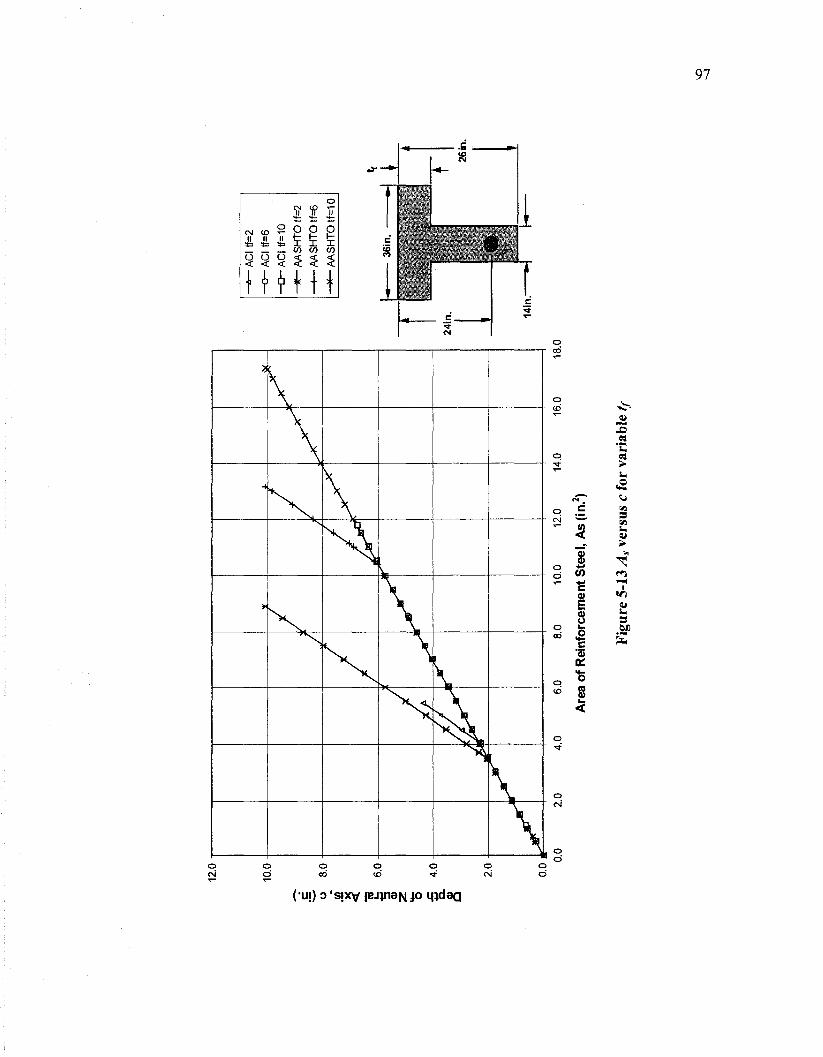
12.0
AC
I tf=
2
AC
I tf=
6
AC
I tf=
10
AA
SH
TO
tf=2
MS
HT
Otf
=6
AA
SH
TO
tf=10
Are
a of
Rei
nfor
cem
ent
Ste
el, A
s (i
n.)
Fig
ure
5-13
As
vers
us c
for
vari
able
tf
•O

98
5.2 STM
Five deep beams previously tested by Ha were reevaluated using the Strut and Tie
Method (STM) as described by both the ACI 318-08 and AASHTO LRFD code
provisions.
Section geometry and variables are shown in Figure 5-14 and Table 5.4.
12in.
36in.
OPEN
4in. l-^—
-12ia-
40in.
A 44in.
4in.
Figure 5-14 Generic beam with and without opening
Table 5-4 Cutout locations from lower left corner in inches
12in. x 12in. Cutout Location ^ - ^ ^
SERIES 1 SERIES 2 SERIES 3 SERIES 4 SERIES 5
X N/A 16 16 16 20
y N/A 12 8 16 12

99
5.2.1 Maximum Allowable Concentrated Load - STM versus FEA
In the work performed by Ha the maximum test loads applied to the sections
varied from 70kips to 175kip depending on the beam geometry. All design loads and
their corresponding ACI 318-08 and AASHTO LRFD counterparts are summarized in
Table 5-5 and are shown graphically in Figure 5-15. The gray columns in Table 5-5
represent the STM method predicted loads as a percentage of Ha's test loads.
Table 5-5 Predicted load versus maximum test load comparisons
SERIES 1 2 3 4 5
Ha 175.00 125.00 150.00 70.00 100.00
ACI 318-08 127.96 85.68 106.35 73.53 86.67
% 73.12 68.54 70.90
105.04 86.67
AASHTO - LRFD 119.43 79.97 99.26 68.63 80.89
% 68.25 63.98 66.17 98.04 80.89
A% 4.87 4.57 4.73 7.00 5.78
Of the five comparisons made only series 4 produced predicted load values that
exceeded the test load used by Ha; this was only true when the ACI 318-08 code
provisions were utilized and this exceedance was 5.04%. The magnitude of the predicted
loads calculated using the AASHTO LRFD in series 4 were 98.04% of the actual test
load value used by Ha of 70 ksi. The predicted values for all other cases analyzed were
well below the experimental test loads used by Ha; this was consistent with expectations
given the conservative nature of the STM model process.
In the instance of series 4 several factors can explain the fact that the predicted
safe design load inclusive of safety factors was greater than the load actually reached

100
during Ha's laboratory testing. Analytical and predictive calculations make several
assumptions any of which can be the source of this discrepancy:
• compressive strength of concrete is consistent throughout the section
• placement of the concrete is without voids or inconsistencies
• area and depth of reinforcement are exact
• cross section geometry and member length are exact
In every series the maximum load the beam was predicted to be capable of
carrying was greater when the ACI 318-08 code was used. The load predicted as
analyzed using AASHTO LRFD was always 93.3% of that analyzed using ACI 318-08.
When a comparison was made between the area of reinforcing steel required by each
code the AAHSTO-LRFD code requirement was 77.8% of that of the ACI 318-08
sections. Reference Equations 5-7 and 5-8. These percentages were directly attributable
to the different values specified for the strength reduction factors by each code.
%Load Mcnn-m </>AASHTO-LRFD
0 / . J ^ C / 3 1 8 - 0 8 _ „ , , - , 0.75 ___ %Loaa— =>93.3 = 77.8 (5-8)
0AASHTO-LRFD 0.9
5.2.2 Maximum Allowable Concentrated Load without </> - STM versus FEA
A second comparison was made between the experimental design loads used by
Ha and the analytical results derived in this paper without application of the strength
reduction factor ^. All design loads and their corresponding ACI 318-08 and AASHTO

101
LRFD counterparts without the application of </> are summarized in Table 5-6 and are
shown graphically in Figure 5-16. Again the gray columns in Table 5-5 represent the
STM method predicted loads as a percentage of Ha's test loads.
Table 5-6 Predicted load without # versus maximum test load comparisons
SERIES
1 2 3 4 5
T.H.
175.00 125.00 150.00 70.00 100.00
ACI 318-08
170.62 114.24 141.79 98.04 115.56
%
97.50 91.39 S4<53
140.06 118.56
AASHTO -LRFD
170.62 114.24 141.79 98.04 115.56
,l
m ' mmi
A%
0.00 0.00 0.00 0.00 0.00
In the cases of both series 4 and 5 it can be observed that the predicted strengths
have exceeded the actual test loads as determined by Ha. This finding clearly
demonstrates the importance of using the strength reduction factor to account for any
imperfections during the mixing and placement of concrete as well as the location of
reinforcing steel.
The removal of the strength reduction factors also illustrated the significance of
largest difference between the ACI 318-08 and AASHTO LRFD when using the method
of strut and tie models as shown in Table 5-6. The strength reduction factors assigned by
the ACI 318-08 and AASHTO LRFD codes are very different from each other and
therefore would never produce identical results for the same section same regardless of
truss or member geometry; only by ignoring the contribution of the strength reduction
factors altogether could identical results be achieved for each code.

Load Comparison
140.00
120.00
Load Values
80.00
0.00
IT. Ha's Loads IACI 318-08 Loads IAASHTO-LRFD Loads
Figure 5-15 Predicted load vs. maximum test load comparisons
Load Comparison Without 4
T. Ha's Loads ACI 318-08 Loads AASHTO - LRFO Loads
Figure 5-16 Predicted load without i vs. maximum test load comparisons

103
6.0 SUMMARY and CONCLUSIONS
6.1 Summary
Twelve different flanged shallow beam sections were designed and analyzed for
flexural resistance by applying both the ACI 318-08 and the AASHTO LRFD code
provisions using hand calculations and analytical software developed by the author. An
additional five rectangular deep beam sections were analyzed using the method of strut
and tie models by applying both the ACI 318-08 and AASHTO LRFD code guidelines,
utilizing Pro/E CAD software, hand calculations and analytical software developed by the
author. Flexural shallow beam sections were divided into four categories; each category
represented a geometric feature to be varied; flange width b, flange depth t/, web width
bw, and the depth of the centroid of reinforcement dt. Factored moment capacity M,„ for
each section was calculated for reinforcing steel amounts that were increased by
increments of 0.50 square inches. The deep beam sections investigated were identical,
apart from the inclusion and location of a 12in. x 12in. opening. Maximum load capacity
was predicted for a concentrated load located at the center on the top face of the beam.
Differences found between the code provisions included but were not limited to
the method prescribed for finding the allowable limits of reinforcement or the method
used for determining the location of the neutral axis. Many other differences existed but
would only be noticed if prestressed reinforcement was incorporated into the design; this
fell beyond the scope of this study. The methods employed to reach solutions for both

104
sets of problems could vary greatly between the two codes however there were no
significant differences in the end results derived from using either set of provisions.
6.2 Conclusion
6.2.1 Asmin and Asmax for Flexure
Web width bw, had the greatest impact upon the minimum allowable
reinforcement for a given section; whereas the minimum allowable reinforcement Asmin,
and the flange depth t/, had the greatest influence upon the maximum allowable
reinforcement Asmax for a section.
6.2.2 As versus Mu for Flexure
Web width bw, had the greatest effect on a given section's moment capacity
regardless of what code was utilized. Significant differences were encountered between
the ACI 318-08 and AASHTO LRFD provisions when analyzing or designing sections
for moment capacity in regards to the method prescribed for finding the allowable limits
of reinforcement. In spite of these differences the results obtained from both codes for all
cases analyzed within this paper were always within 1.4% of each other.
6.2.3 Depth of Neutral Axis c for Flexure
The method for calculating the depth of the neutral axis c, was the most
noticeable difference between the ACI 318-08 and AASHTO LRFD code provisions.
However the results calculated for sections from either code discussed in this paper were

105
never more than 9% apart. This was attributed to the fact that only non-prestressed, plain
reinforced sections were analyzed. Results using non-reinforced sections were never
considered for this thesis.
6.2.4 Strength Reduction Factor $ for Flexure
Due to the limits of reinforcement placed each section by both codes, the strength
reduction factor, <f>, was always equal to 0.9 and therefore <j) did not have a differing affect
on the results obtained from either code.
6.2.5 Maximum Load Capacityfor STM
Maximum predicted load capacity for any of the beam series studied was always
greater when analyzed using the ACI 318-08 Appendix A STM method provisions than
when using the AASHTO LRFD provisions. These differences in maximum predicted
load capacity ranged from 4.57% to 7.00%. Inherent differences in member effectiveness
factors and the strength reduction factors were the source of this variance.

106
Works Cited
ACI Committee 318. Building Code Requirements for Structural Concrete 318-02, and Commentary (318R-02). Farmington Hills. American Concrete Institute. 2002.
I ACI Committee 318. Building Code Requirements for Structural Concrete 318-08, and
Commentary (318R-08). Farmington Hills. American Concrete Institute. 2005.
American Association of State Highways and Transportation Officials, AASHTO LRFD. AASHTO LRFD Bridge Design Specifications. 3rd ed. Washington DC. 2004.
Beres, Attila. Notes on ACI 318-02 Building Code Requirements for Structural Concrete with Design Applications. 8th ed. Portland Cement Association. Skokie, IL. 2002.
Brown, Michael D., Sankovich et al. "Behavior and Efficiency of Bottle Shaped Struts." ACI Structural Journal 103.3 (2006): 348-55.
Foster, Stephen J., and Adrian R. Malik. "Evaluation of Efficiency Factor Models used in Strut-and-Tie Modeling of Nonflexural Members." Journal of Structural Engineering 128.5 (2002): 569-77.
Gupta, Pawan R., and Michael P. Collins. "Evaluation of Shear Design Procedures for Reinforced Concrete Members under Axial Compression." ACI Structural Journal 100.4 (2001): 537-47.
Ha, Sun Thuc. Design of Concrete Deep Beams with Openings and Repair Using Carbon Fiber Laminates. San Jose State University. San Jose, CA. 2002.
Hibbeler, R.C. Mechanics of Materials. 6th ed. Upper Saddle River, NJ. Pearson; Prentice Hall. 2005.
Hsu, Thomas T. C, "Toward a Unified Nomenclature for Reinforced-Concrete Theory." Journal of Structural Engineering 122.3 (1996): 275-83.
Kamara, Mahmoud E., and Basile G. Rabbat. Notes on ACI 318-05 Building Code Requirements for Structural Concrete with Design Applications 9th ed. Portland Cement Association. Skokie, IL. 2005.
Leet, Kenneth M., and Chia-Ming Uang. Fundamentals of Structural Analysis. 1st ed. New York. McGraw-Hill. 2002.
107
Leu, Liang-Jeng, Huang, et al. "Strut-and-Tie Design Methodology for Three-Dimensional Reinforced Concrete Structures." Journal of Structural Engineering 132.6 (2006): 929-38.
MacGregor, James G. Reinforced Concrete - Mechanics and Design. 3rd ed. Englewood Cliffs, NJ. Pretence Hall. 1997.
McCormac, Jack C, and James K. Nelson. Design of Reinforced Concrete ACI 318-05 Code Edition. 7th ed. Hoboken, NJ. Wiley. 2006.
Naaman, Antoine E. Prestressed Concrete Analysis and Design Fundamentals. 2" ed. Ann Arbor, MI. Techno Press 3000. 2004.
Naaman, Antoine E. Limits of Reinforcement in 2002 ACI Code: Transition, Flaws, and Solution. ACI Structural Journal 101.2 (2004): 209-18.
Rahal, Khaldoun N., and Khaled S. Al-Shaleh. "Minimum Transverse Reinforcement in MPa Concrete Beams." ACI Structural Journal 101.6 (2004): 872-78.
Rahal, Khaldoun N., and Michael P. Collins. "Experimental Evaluation of ACI and AASHTO LRFD Design Provisions for Combined Shear and Torsion." ACI Structural Journal 98.4 (2003): 277-82.
Reineck, Karl-Heinz. Examples for the Design of Structural Concrete with Strut and Tie Models. American Concrete Institute. Farmington Hills, MI. 2002.
Tan K. H., and G.H. Cheng. "Size Effect on Shear Strength of Deep Beams: Investigating with Strut-and-Tie Model." Journal of Structural Engineering 132.5 (2006): 673-85.
Wright, James T., and Gustavo J. Parra-Montesinos. Strut and Tie Model for Deep Beam Design - A Practical Exercise using Appendix A of the 2002 ACI Building Code. Concrete International. 2003.
Zwicky, Daia, and Thomas Vogel. "Critical Inclination of Compression Struts in Concrete Beams." Journal of Structural Engineering 132.5 (2006): 686-93.

App
endi
x A
- D
eep
Bea
m S
TM
Mod
els
SE
RIE
S 1
MEM
BER
1 2 i
MIN
IMU
M
WID
TH
4.01
1
5.41
5.4
1
Fig
ure
A -
1 D
eep
beam
ser
ies
1 ST
M m
odel
o

Loa
d P
SERI
ES 2
MEMBER
1
2
3
4
5
6
7 «
9
MINIMUM
UNIH
H 5 62
4.00
5.62
4,00
5.64
5.64
4.00
4.00
4.00
Fig
ure
A -
2 D
eep
beam
ser
ies
2 ST
M m
odel
o
v©
I

SE
RIE
S J
MEM
BER
1 Z 3 4 5 6 7 9 i
MIN
IMU
M
WID
TH
5.&
0
4.00
5. so
4.00
5.84
5.64
4.00
4.00
4.00
Fig
ure
A -
3 D
eep
beam
ser
ies
3 S
TM
mod
el

SERI
ES 4
MEMBER
1
Z
3
4
5
6
7
9 $
MINI
MUM
KIHT
H
5.63
4.00
5.53
4.00
5. U
5.24
4.00
4.00
3.59
Fig
ure
A -
4 D
eep
beam
ser
ies
4 ST
M m
odel

Lo
ad
SERI
ES 5
MEMB
ER
1
2
3
4
5
6
1 e
3
MINIMUM
WIDT
H
5.62
4.O0
5.62
3.63
5.38
5.38
3,S3
4.47
4.00
Fig
ure
A -
5 D
eep
beam
ser
ies
5 ST
M m
odel
K>

App
endi
x B
- D
eep
Bea
m S
TM
Tru
ss M
odel
s
Loa
d P
36. C
O
O
T
Fig
ure
B -
1 D
eep
beam
ser
ies
1 S
TM
tru
ss m
odel

12.C
O-
IO.D
O-
2.0
5-
Lo
ad
P 5
OPE
N
Fig
ure
B -
2 D
eep
beam
ser
ies
2 S
TM
tru
ss m
odel

OPE
N
Fig
ure
B -
3 D
eep
beam
ser
ies
3 ST
M t
russ
mod
el

Lo
ad
P s
16. 0
0 -
14. 0
0 -
2.0
0-
.go
-
OPE
N
Fig
ure
B -
4 D
eep
beam
ser
ies
4 ST
M t
russ
mod
el
CT
s
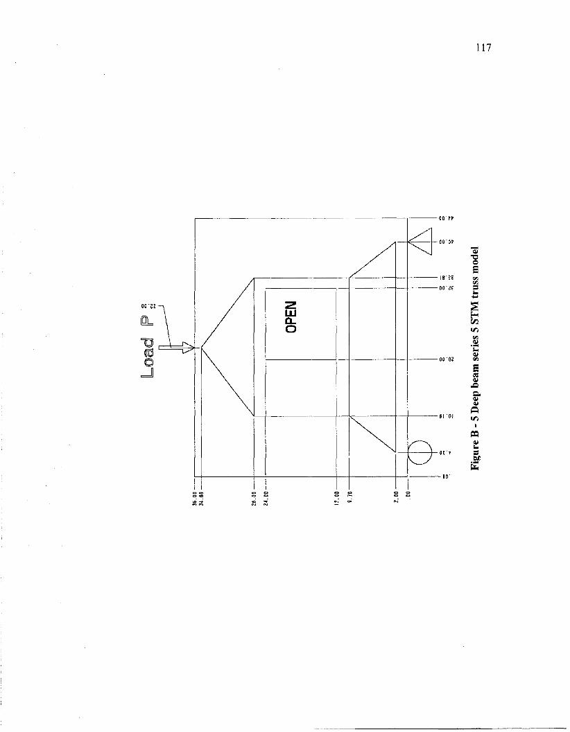
Load
34
.89
-
26
.00
-
24
.00
-
12
.00
-
8.7
6-
.00
-
OPE
N
Fig
ure
B -
5 D
eep
beam
ser
ies
5 S
TM
tru
ss m
odel
-~
j

36.
CO
26
.83 F
igur
e B
- 6
Dee
p be
am s
erie
s 5a
Alt
erna
te S
TM
tru
ss m
odel

Appendix C - STM Truss Free Body Diagrams & Solutions
Deep beam series 1 free body diagram and solution
34.0
Truss Element 1 2 3
Element Force 0.566 C 0.464 T 0.566 C
^ + IMA =0=>RB* 36m.-1 = 0 RR= 0.500
t +IFr = 0 => RA + 0.500 - 1 = 0
RA =0.500
9a
a JL
0.500
F2
34 0= tan"1 — =>0 =62.10°
18 t +2Fr = 0 => 0.500 - Fx sin 62.10° = 0
Fl = 0.566 -> +SFX = 0 => F2 -0.566 cos 62.10° = 0
F2 = 0.468
From symmetry Ft = F3.". F3 = 0.566

Deep beam series 2 free body diagram and solution
24.0
33.14
0.0 10.0 18.0 26.0 36.0
£+2MA = 0 => RB*36in.-l = 0
RB= 0.500
t+LF r = 0 => +0.500-1 = 0 RA = 0.500
Truss Element 1 2 3 4 5 6 7 8 9
Element Force 0.800 C 0.625 T 0.800 C 0.500 C 0.664 C 0.664 C 0.500 C 0.625 C 0.437 T

6 = tan"1 — z*9 =38.66° 10
t+SF r = 0=> 0.500-F, sin 38.66° = 0 Fx = 0.800
-> +EFX = 0 => F2 -0.800cos38.66° = 0 F2 = 0.625
t +SF7 = 0 => 0.800sin38.66°- F7 = 0
F1 = 0.500
-> +1LFX = 0 => 0.800 cos 38.66° - F8 = 0
FQ = 0.625
0, = tan-1 — =>0f =48.81° 7 8.0 f
t +2Fr = 0=> 0.500 -F6 sin 48.81° = 0
F6 = 0.664
-> +HFX = 0 => F9 -0.664 cos 48.81° = 0
F9 = 0.437
From symmetry F, = F3, F4 = F1 & F5 = F6
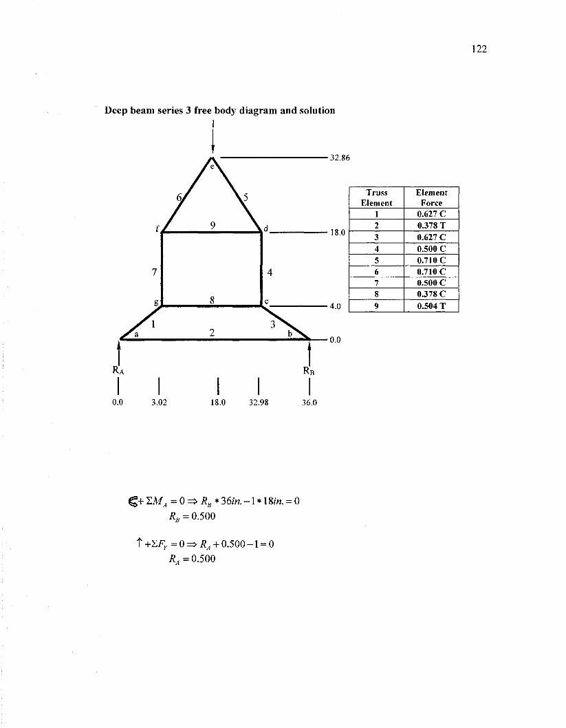
Deep beam series 3 free body diagram and solution
32.86
Truss Element
1 2 3 4 5 6 7 8 9
Element Force
0.627 C 0.378 T 0.627 C 0.500 C 0.710 C 0.710 C 0.500 C 0.378 C 0.504 T
RA
•0.0
RB
0.0 3.02 18.0 32.98 36.0
^ + TMA = 0 => RB * 36m. - 1 * 18w. = 0
RB = 0.500
t +ZFY = 0 => RA + 0.500 -1 = 0 ^ = 0 . 5 0 0
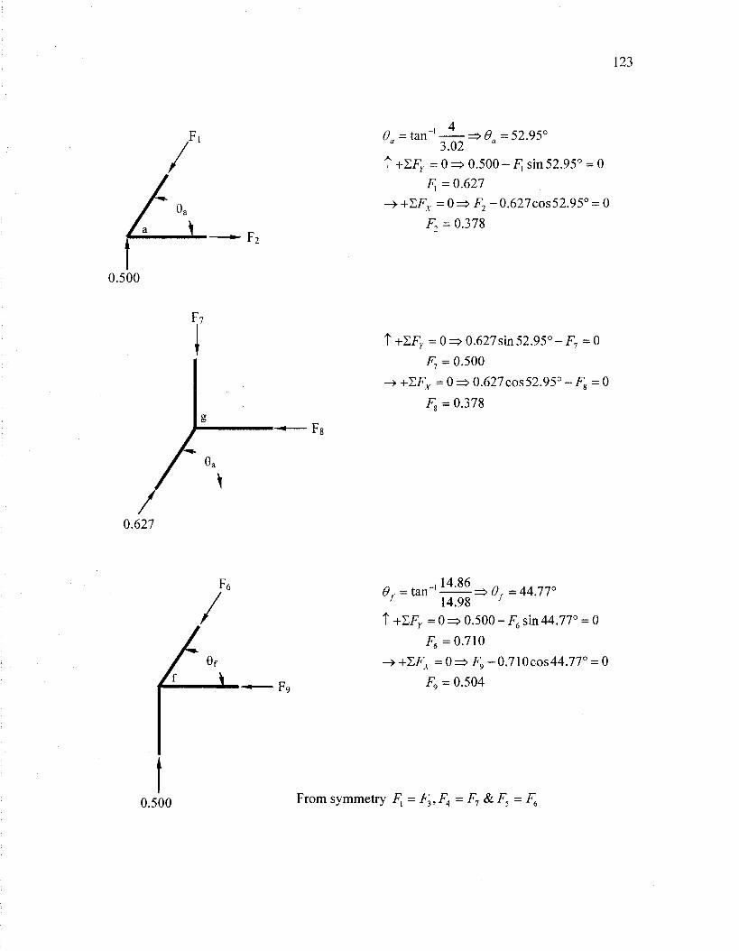
F8
6n = tan-1 — =>0a- 52.95° 3.02
t +ZFr = 0 => 0.500 - F sin 52.95° = 0 Y
Fx = 0.627
-» +SFX = 0 => F2 - 0.627cos52.95° = 0
F2 = 0.378
t +EFr = 0 => 0.627 sin 52.95° - Fn = 0
F7 - 0.500
->+EFx = 0^0.627 cos 52.95° - F 8 = 0
Fa = 0.378
ef = tan-1 ^ ^ =* 0, = 44.77° f 14.98 r
t +Siv = 0 => 0.500 - F6 sin 44.77° = 0
F6= 0.710
-» +EFX = 0 => F9 -0.710cos44.77° = 0
Fg = 0.504
From symmetry Fl = F3, F4 = F1 & F5 = F6

Deep beam series 4 free body diagram and solution
124
32.77
27.85
12.0
Truss Element
1 2 3 4 5 6 7 8 9
Element Force
0.651 C 0.417 T 0.651 C 0.500 C 0.954 C 0.954 C 0.500 C 0.417 C 0.813 T
26.0 36.0
^ + T,MA =0=>RB* 36m.-1 = 0
RB = 0.500
t +ZFr = 0 => + 0.500-1 = 0 RA = 0.500

0= tan-1 — =$0= 50.19° 10
t +EF r=0=> 0.500- F, sin 50.19° = 0
F, =0.651 ->+LFy = 0 ^ F 2 - 0 . 6 5 lcos50.19° = 0
F2= 0.417
t+SF r =0^0.651s in50.19°-F 7 =0
F7 = 0.500
->+EFA.=0=>0.651cos50.19°-Fg=0
F, =0.417
, 4 92 0t= tan-1 - ^ = > 0 , =31.59° 7 8.0 7
t +SFK = 0 z=> 0.500 - F6 sin 31.59° = 0
F6 = 0.954
-> +SFX = 0 => F9 - 0.954 cos 31.59° = 0
F9 = 0.813
From symmetry Ft = F3, F4 = F7 & F5 = F6

Deep beam series 5 free body diagram and solution
Truss Element
1 2 3 4 5 6 7 8 9
Element Force
0.640 C 0.399 T 0.640 C 0.500 C 0.831 C 0.831 C 0.500 C 0.399 C 0.664 T
18.0 29.81 36.0
^ + ZMA = 0=>RB* 36/n.-1 = 0
RB = 0.500
t + S F r =0=>RA +0.500-1 = 0 R, = 0.500

e = tan"1 — ^0= 51.42° 6.19
t+SF r =0=>.500-F,sin51.42° = 0 F, = 0.640
-> +EFy = 0 => F2 - 0.640 cos 51.42° = 0 F2 = 0.399
f +SFr = 0 => 0.640 sin 51.42° - F7 = 0
F7 = 0.500
-> +IF , = 0 => 0.640 cos 51.42° - Fg = 0
Fa = 0.399
o on 0, = tan"1 - ^ - => 0, = 36.97° f 11.81 y
t +ZFr = 0 => 0.500 - F6 sin 36.97° = 0
F6 =0.831
-> +1FX = 0 => F9 - 0.831 cos 36.97° = 0
F9 = 0.664
From symmetry F, = F3,F4 = F7 & F5 = F6