5.5 multiple moving average

Noise Reduction using Moving average Multiple moving average

5.5 Multiple moving average

In the case of applying two times,

gi =∑

m

wmfi−m

hi =∑

m′

wm′gi−m′

(gi−m′ =∑

m

wmfi−m′−m)

=

N∑

m′=−N

N∑

m=−N

wm′wmfi−m′−m

When Nm = 3(N = 1), wm = w′m = 1/3

gi =fi−2 + 2fi−1 + 3fi−1 + 2fi+1 + fi+2

9

0

x′

w(x′)

∆x

N∆x−N∆x

(2N + 1)∆x = Nm∆x

w

Applying multiple moving aver-age is equivalent to moving av-erage with which central weightis larger than neighboring points.

82 / 197

Noise Reduction using Moving average

Spectral Gain of Multiple Moving Average

In the case of two times,

g(x) =

∫ ∞

−∞w(x′)f(x− x′) dx′ → G(k) = W (k)F (k)

h(x) =

∫ ∞

−∞w(x′)g(x − x′) dx′ → H(k) = W (k)G(k)

= W 2(k)F (k)

1 sinc(θ)

sinc2(θ)

θ

(θ = kXm)

0 π 2π 3π−π−2π−3π

Further reduction of higherfrequency components is applied.

No spurious resolution.

83 / 197

Noise Reduction using Moving average Higher order Moving average (Savitzky-Golay filter)

5.6 Higher order Moving average (Savitzky-Golay filter)

For each i,

Represent the smoothed function gi(xj)by a power series expansion.

(j ∈ {i−N, · · · , i+N})(In the case of second order expansion,)

gi(xj) = ai(xj − xi)2 + bi(xj − xi) + ci

= ai∆x2j,i + bi∆xj,i + ci x

gi

fi

fi+1

fi+2

fi−1

fi−2

xi xi+1xi+2xi−1xi−2

Using by the least square method, determin the parameter ai, bi,and ci which are the parameter of the fitting function gi(xj).

The moving average at the point i corresponds to the value of thefitting function at the xj = xi; i.e gi(xi) = ci.

84 / 197


Least square fitting to the parabolic function

Fitting functiongj = a∆x2j + b∆xj + c ((omit i))

Minimize Average of square residual, E:

E(a, b, c) =1

Nm

i+N∑

j=i−N

(gj − fj)2 ≡ (gj − fj)2

minimize E(a, b, c) ⇐⇒ ∂E∂ξ = 0 (ξ ∈ {a, b, c})

(∂E∂ξ = ∂

∂ξ (gj(ξ)− fj)2 = 2(gj(ξ)− fj)∂gj(ξ)∂ξ

∂gj∂a = ∆x2j ,

∂gj∂b = ∆xj,

∂gj∂c = 1

)

∆x4j ∆x3j ∆x2j∆x3j ∆x2j ∆xj

∆x2j ∆xj 1

abc

=

fj∆x2jfj∆xjfj

85 / 197


Least square fitting to the power series

Fitting function

f̃(x;a) =

Nl∑

l=0

alxl,

a = (a0, a1, · · · , aNl)

Sampling points (known)(xi, fi), i ∈ {1, · · · , N}

Minimize Average ofsquare residual, E

E(a) =1

Ni

Ni∑

i=1

(f̃(xi;a)− fi)2

≡ (f̃(xi;a)− fi)2

minimize E(a) ⇔ ∂E

∂al= 0

(∂E∂al

= ∂∂al

(f̃i − fi)2 = 2(f̃i − fi)∂f̃i∂al

= 2(f̃ixli − fixli

)= 0

(∵

∂f̃i∂al

= xl)

)

∴

Nl∑

l=0

xl+mi al = fix

mi

x0 x1 · · · xNl

x1 x2 · · · xNl+1

......

. . ....

xNl xNl+1 · · · xN2l

a0a1...

aNl

=

fix0i

fix1i...

fixNl

i

The parameter of the least square fittingto power series function (non-linear func-tion) can be obtained by solving a set oflinear equations.

86 / 197


Moving average by parabolic fitting

∆x4j ∆x3j ∆x2j∆x3j ∆x2j ∆xj

∆x2j ∆xj 1

abc

=

fj∆x2jfj∆xjfj

In the case of Nm = 5(N = 2)

∆xj = 0, ∆x3j = 0,

∆x2j/∆2 = (−2)2+(−1)2+02+(+1)2+(+2)2

5 = 2(12+22)5 = 2,

∆x4j/∆4 = 2(14+24)

5 = 345

c =

∣∣∣∣∣∣

345 ∆

4 0 fj∆x2j0 2∆2 fj∆xj

2∆2 0 fj

∣∣∣∣∣∣

/∣∣∣∣∣∣

345 ∆

4 0 2∆2

0 2∆2 02∆2 0 1

∣∣∣∣∣∣

=685 ∆

6fj − 4∆4fj∆x2j285 ∆

6

Num. =68[f−2 + f−1 + f0 + f1 + f2]

5∆6

− 4[(−2)2f−2 + (−1)2f−1 + 02f0 + 12f1 + 22f2]∆2

5∆4

= ∆6((

6825 − 16

5

)(f−2 + f+2) +

(6825 − 4

5

)(f−1 + f+1) +

6825f0

)

gi = c

=1

35( −3 12 17 12 −3 )

fi−2

fi−1

fifi+1

fi+2

The weight at point i ismaximum.

The weights at both ends arenegative.

W (k)

k

W (k)

0

1

kmin kmax

W (k) is flat in low frequency.

87 / 197

Noise Reduction using Moving average Gaussian Filter

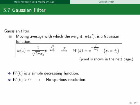
5.7 Gaussian Filter

Gaussian filter:≡ Moving average with which the weight, w(x′), is a Gaussian

function.

w(x) =1√2πσx

e− x2

2σ2x

F=⇒ W (k) = e

− k2

2σ2k

(σk = 1

σx

)

(proof is shown in the next page.)

W (k) is a simple decreasing function.

W (k) > 0 → No spurious resolution.

88 / 197

Noise Reduction using Moving average Gaussian Filter

Fourier Transform of Gaussian function

W (k) = F {w(x)}

=1√2πσx

∫ ∞

−∞e− x2

2σ2x e−ikx dx

(X = x√2σx

)

=1√πe−

σ2x2k2∫ ∞

−∞e−(X+i kσx√

2)2dX

︸︷︷︸=∫e−X2 dX=

√π (∗)

= e−σ2x2k2 = e

− 1

2σ2k

k2

(σk = 1σx)

F{e− x2

2σ2x

}∝ e−

σ2xk2

2

(∗)

I =

∫ ∞

−∞e−(x+ib)2 dx

=

∫ ∞−ib

−∞−ibe−z2 dz

Z

x

y

−R +R

−ibc(R → ∞)

(No poles)∫

ce−z2 dz = 0 → I =

∫ ∞

−∞e−x2

dx

I2 =

∫ ∞

−∞

∫ ∞

−∞e−(x2+y2) dx dy

=

∫ 2π

0

∫ ∞

0e−r2r dθ dr (t = r2)

= −π[e−t]∞0

= π

∴ I =√π

89 / 197

Noise Reduction using Moving average Cummulative Average of muliple measurement

5.8 Cummulative Average of muliple measurement

Nk sets of measurement.f(k)i = f̃i + n

(k)i

(k ∈ {1, · · · , Nk})

Cummulative Ave.

〈〈yi〉〉 ≡1

Nk

Nk∑

k=1

y(k)i

Cummul. Ave. of figi = 〈〈fi〉〉 = f̃i + 〈〈ni〉〉

Expected value : E [gi]

E [gi] = f̃i + E [〈〈ni〉〉]︸︷︷︸=〈〈E[ni]〉〉=0= f̃i

Variance of gi : σ2gi (※ 6= Var. of fi)

σ2gi = E

[(gi − E [gi])

2]= E

[{(f̃i + 〈〈ni〉〉)− f̃i

}2]

= E[〈〈ni〉〉2

]= E

[1

N2k

∑

k

∑

k′

n(k)i n

(k′)i

]

= E

[1

N2k

∑

k

((n(k)i

)2+∑

k′ 6=k

n(k)i n

(k′)i

)]

=

∑

k

σ2n︷︸︸︷

E

[(n(k)i

)2]

N2k

+

∑

k

∑

k′ 6=k

0︷︸︸︷E[n(k)i n

(k′)i

]

N2k

=1

N2k

Nk∑

k=1

σ2n =

σ2n

Nk

√σ2gi is called standard error.

90 / 197

Noise Reduction using Moving average Cummulative Average of muliple measurement

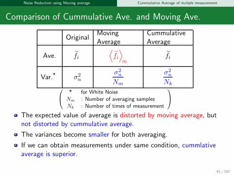
Comparison of Cummulative Ave. and Moving Ave.

OriginalMovingAverage

CummulativeAverage

Ave. f̃i

⟨f̃i

⟩m

f̃i

Var.* σ2n

σ2n

Nm

σ2n

Nk

* for White NoiseNm : Number of averaging samplesNk : Number of times of measurement

The expected value of average is distorted by moving average, butnot distorted by cummulative average.

The variances become smaller for both averaging.

If we can obtain measurements under same condition, cummlativeaverage is superior.

91 / 197

Noise Reduction using Moving average Propagation of Error

5.9 Propagation of Error

Two independent measurements, f and g (|df | ≪ |f̃ |, |dg| ≪ |g̃|) :

f = f̃ + df, E [f ] = f̃ , E [df ] = 0, E[(df)2

]= σ2

f

g = g̃ + dg, E [g] = g̃, E [dg] = 0, E[(dg)2

]= σ2

g

Consider evaluetion of a new result : h ≡ h(f, g) = h̃(f, g) + dh(f, g)

Average:

dh =∂h

∂f

∣∣∣∣(f̃ ,g̃)

df +∂h

∂g

∣∣∣∣(f̃ ,g̃)

dg

= h′fdf + h′gdg

E [dh] = h′fE [df ] + h′gE [dg]

= 0

E [h] = E[h̃+ dh

]= h̃(f̃ , g̃)

Variance:σ2h = E

[(dh)2

]= E

[(h′fdf + h′gdg

)2]

= h′f2E[df2]

︸︷︷︸σ2f

+h′g2E[dg2]

︸︷︷︸σ2g

+2h′fh′g E [df · dg]︸︷︷︸

=0

=

(∂h

∂f

∣∣∣∣h̃

)2

σ2f +

(∂h

∂g

∣∣∣∣h̃

)2

σ2g

92 / 197

Noise Reduction using Moving average Propagation of Error

Example of Error Propagation

h ≡ h(f, g)

σ2h =

(∂h∂f

∣∣∣h̃

)2σ2f +

(∂h∂g

∣∣∣h̃

)2σ2g

Add. and Sub.◮ h = f + g

σ2h = σ2

f+g = σ2f + σ2

g◮ h = f − g

σ2h = σ2

f−g = σ2f + σ2

g

Sum of each Variance.

Mul. and Div.◮ h = f · g

σ2h = σ2

f ·g = g2σ2f + f2σ2

g

σ2h

h2=

σ2f

f2+

σ2g

g2◮ h = f/g

σ2h = σ2

f/g = 1

g2 σ2f + f2

g4 σ2g

σ2h

h2=

σ2f

f2+

σ2g

g2

Sum of each normalized Variance.

93 / 197

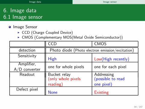
Image data Image sensor

6. Image data6.1 Image sensor

Image Sensor◮ CCD (Charge Coupled Device)◮ CMOS (Complementary MOS(Metal Oxide Semiconductor))

CCD CMOS

detection Photo diode (Photo electron emission/excitation)

SensitivityHigh Low(High recently)

Amplifier,A/D converter

one for whole pixels one for each pixel

Readout Bucket relay Addressing(only whole pixelsreading)

(possible to readone pixel)

Defect pixelNone Existing

94 / 197


CCD

Circuit Bucket Relay

V (t0)

V (t1)

V (t2)

V (t3)

V (t4)

Photo diode

95 / 197


CMOS

Circuit

96 / 197


Color Camera

three chips (high quality)

Separating color by using prisms,each of which can reflect acertain color. Separated beamsare detected each sensor.

R

G

B

one chip (small size)

Color filter is placed in front ofsensor.

97 / 197

Image data Signal to Noise ratio and Resolution

6.2 Signal to Noise ratio and Resolution

Charge accumuration by photodiode

iin(t)

vout(t)

I(t)

C SW

PD

Incident Light I(t) ∝ iin(t)◮ SW=ON(close) : vout(t) = 0◮ SW=OFF(Open) (t = [0, T ])

vout(T ) =1

C

∫ T

0iin(t) dt

If I(t) = I (const.),vout(T ) = kIT .

Signal is proportional to T .

I includes fluctuation :I(t) = I + δI(t) → I ± σδIδvout(T ) = k

∫ T0 δI(t) dt

1T

∫ T0 δI(t) dt = 〈〈δI〉〉≡ Cummul. ave. of δI(t)

σ〈〈δI〉〉 ∝ σδI/√T (δI is white)

σvout(T ) = Tσ〈〈δI〉〉 = k′σδI√T

Noise is proportional to√T .

Signal to Noise Ratio S/N :S/N ∝

√T

The quality of signal increaseswith increasing T .

98 / 197

Image data Signal to Noise ratio and Resolution

Area of Pixel A

iin(t) ∝∫

AI(t, x, y) dA

◮ I(t, x, y) = I :vout(A) = kIA

vout is proportional to A.

◮ I(t, x, y) = I + δI(t, x, y) :δvout = k

∫A δI(t, x, y) dA

σ〈〈δI〉〉 ∝ σδI/√A

σvout(A) = k′σδI

√A

vout is proportional to√A.

Signal to Noise Ratio S/N :S/N ∝

√A

The quality of signal increaseswith increasing pixel size A.

Resolution

◮ Temporal resolution ⇔Exposuretime

◮ Spatial resolution ⇔Pixel Size

S/N ResolutionLargeris better

Smalleris better

time ∝√T T

space ∝√A

√A

99 / 197

Image data Discretization and Quantization

6.3 Discretization and Quantization

Discretization and QuantizationContinuous functionf(x)

(x ∈ R, f(x) ∈ R)

◮ Discretization:(Digitizing Domain)xn = n∆x, n ∈ Z

◮ Quantization:(Digitizing Range of f)fm = m∆f , m ∈ Z

Image Data◮ Pixel : Discrete point

⇔ i, j ∈ Z

(e.g. 640×400, 1024×768)

◮ Intensity : Quantized ofbrightness

⇔ Ii,j ∈ Z

A/D (Analog to Digital) converter

e.g.8bits (0,· · · , 255)

10bits (0,· · · , 1023)12bits (0,· · · , 4095)

100 / 197

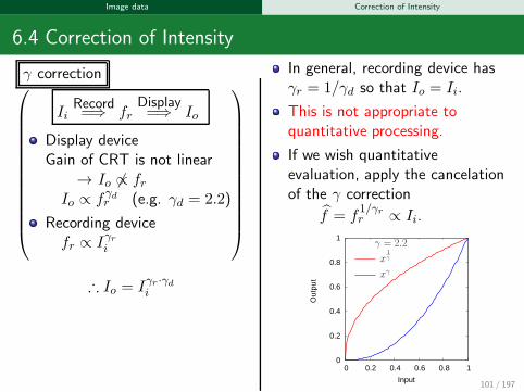
Image data Correction of Intensity

6.4 Correction of Intensity

γ correction

IiRecord=⇒ fr

Display=⇒ Io

Display deviceGain of CRT is not linear

→ Io 6∝ frIo ∝ fγd

r (e.g. γd = 2.2)

Recording devicefr ∝ Iγri

∴ Io = Iγr ·γdi

In general, recording device hasγr = 1/γd so that Io = Ii.

This is not appropriate toquantitative processing.

If we wish quantitativeevaluation, apply the cancelationof the γ correction

f̂ = f1/γrr ∝ Ii.

0

0.2

0.4

0.6

0.8

1

0 0.2 0.4 0.6 0.8 1

Out

put

Input

γ = 2.2

xγx

1γ

101 / 197

Image data Image format

6.5 Image format

Single format

Format Name Color bit Compres. Revers. Multi-image

PBM Portable Bit Map White/Black 1 × ○ ×PGM Portable Gray Map Gray 8 × ○ ×PPM Portable Pixel Map RGB 3×8 × ○ ×GIF Graphics Interchange

FormatRGB 3×8 ○ ○ ○

JPEG Joint PhotographicExperts Group

RGB 3×8 ○ × ×

PNG Portable NetworkGraphics

RGB-alpha∗ 4×16 ○ ○ ×

* : alpha is a channel for transparency

Integrated Multiple formatsFormat Name

PNM Portable aNy Map (PBM, PGM, PPM)

TIFF Tagged Image File Format

BMP Microsoft windows BitMaP

102 / 197

5.5 multiple moving average

Documents