559

Fish 559; Lecture 5

Non-linear Minimization

559

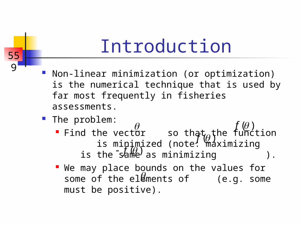
Introduction Non-linear minimization (or optimization) is

the numerical technique that is used by far most frequently in fisheries assessments.

The problem: Find the vector so that the function

is minimized (note: maximizing is the same as minimizing ).

We may place bounds on the values for some of the elements of (e.g. some must be positive).

( )f ( )f

( )f

559

Minimizing a Function-I By definition, for a minimum:

This problem statement is deceptively simple. There is no perfect algorithm. The art of non-linear minimization is to know which method to use and how to determine whether your chosen method has converged to the correct solution.

( )0

opt

f

559

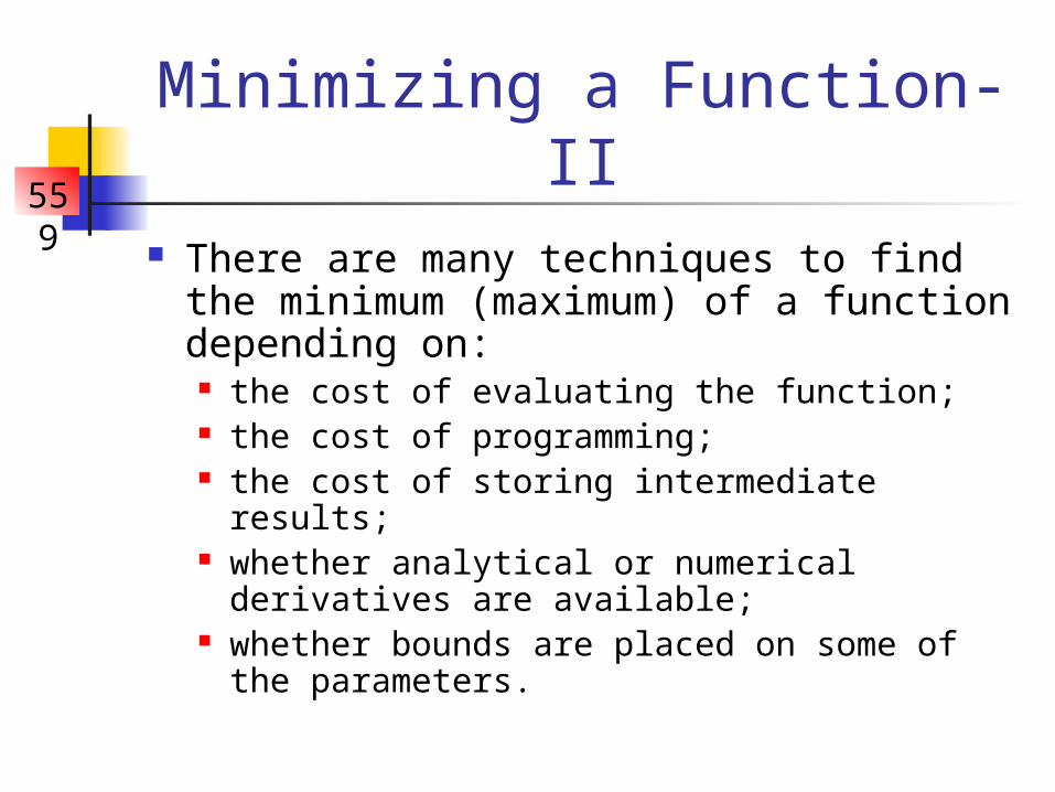
Minimizing a Function-II There are many techniques to find the

minimum (maximum) of a function depending on: the cost of evaluating the function; the cost of programming; the cost of storing intermediate results; whether analytical or numerical derivatives

are available; whether bounds are placed on some of the

parameters.

559

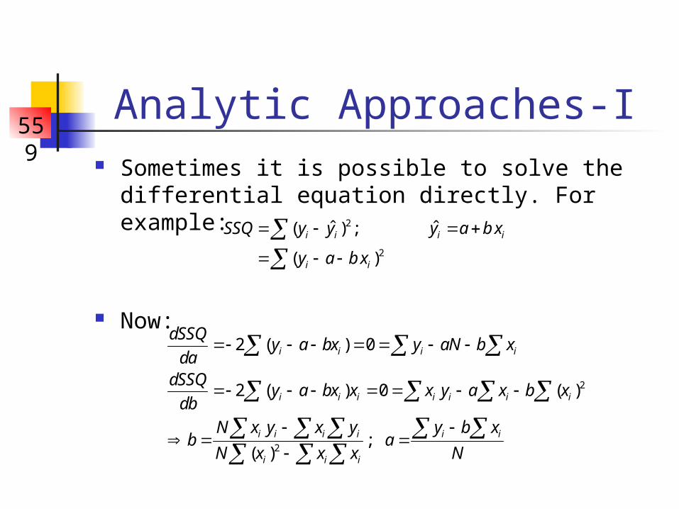
Analytic Approaches-I Sometimes it is possible to solve the

differential equation directly. For example:

Now:

2

2

ˆ ˆ( ) ;

( )

i i i i

i i

SSQ y y y a b x

y a b x

2

2

2 ( ) 0

2 ( ) 0 ( )

;( )

i i i i

i i i i i i i

i i i i i i

i i i

dSSQy a bx y aN b x

dadSSQ

y a bx x x y a x b xdb

N x y x y y b xb a

N x x x N

559

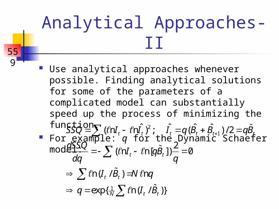
Analytical Approaches-II Use analytical approaches whenever possible.

Finding analytical solutions for some of the parameters of a complicated model can substantially speed up the process of minimizing the function.

For example: q for the Dynamic Schaefer model:

21

1

ˆ ˆ ˆ ˆ( n n ) ; ( ) / 2

2( n n[ ]) 0

n( / ) n

exp{ n( / )}

t t t t t t

t t

t t

t tN

SSQ I I I q B B qB

dSSQI qB

dq q

I B N q

q I B

559

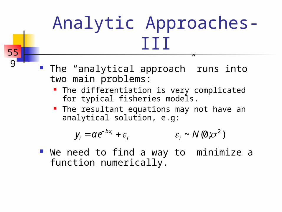
Analytic Approaches-III The “analytical approach” runs into two

main problems: The differentiation is very complicated for

typical fisheries models. The resultant equations may not have an

analytical solution, e.g:

We need to find a way to minimize a function numerically.

2~ (0; )ib xi i iy a e N

559

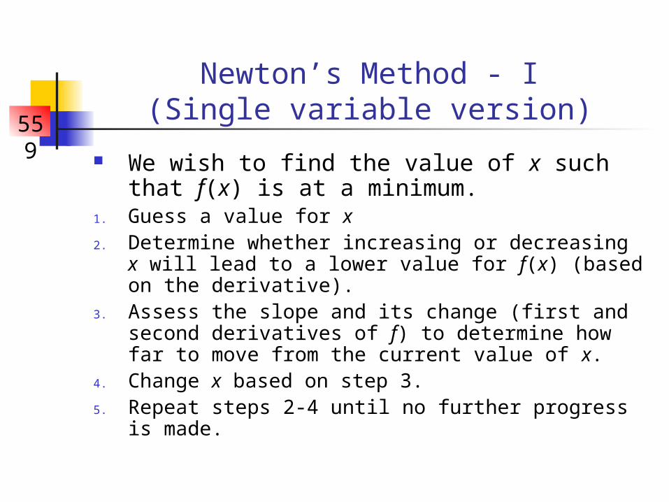
Newton’s Method - I(Single variable version)

We wish to find the value of x such that f(x) is at a minimum.

1. Guess a value for x2. Determine whether increasing or decreasing x

will lead to a lower value for f(x) (based on the derivative).

3. Assess the slope and its change (first and second derivatives of f) to determine how far to move from the current value of x.

4. Change x based on step 3.5. Repeat steps 2-4 until no further progress is

made.

559

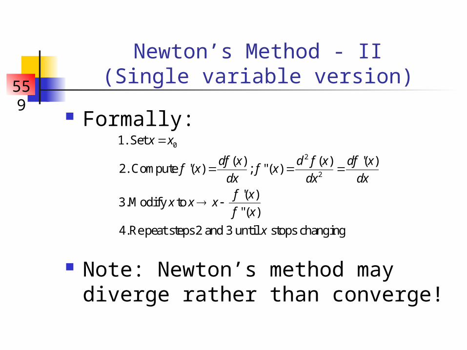
Newton’s Method - II(Single variable version)

Formally:

Note: Newton’s method may diverge rather than converge!

0

2

2

1. Set

( ) ( ) '( )2. Compute '( ) ; "( )

'( )3.Modify to

"( )

4.Re peat steps 2 and 3 until stops changing

x x

df x d f x df xf x f x

dx dx dxf x

x x xf x

x

559

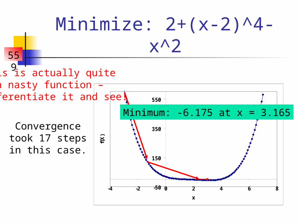
Minimize: 2+(x-2)^4-x^2

-50

150

350

550

-4 -2 0 2 4 6 8

x

f(X

)

This is actually quite a nasty function –

differentiate it and see!

Convergence took 17 steps in this case.

Minimum: -6.175 at x = 3.165

559

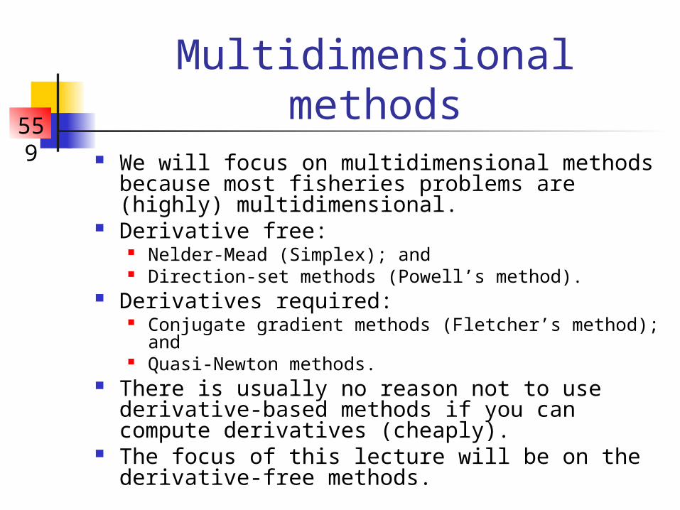
Multidimensional methods We will focus on multidimensional methods

because most fisheries problems are (highly) multidimensional.

Derivative free: Nelder-Mead (Simplex); and Direction-set methods (Powell’s method).

Derivatives required: Conjugate gradient methods (Fletcher’s method);

and Quasi-Newton methods.

There is usually no reason not to use derivative-based methods if you can compute derivatives (cheaply).

The focus of this lecture will be on the derivative-free methods.

559

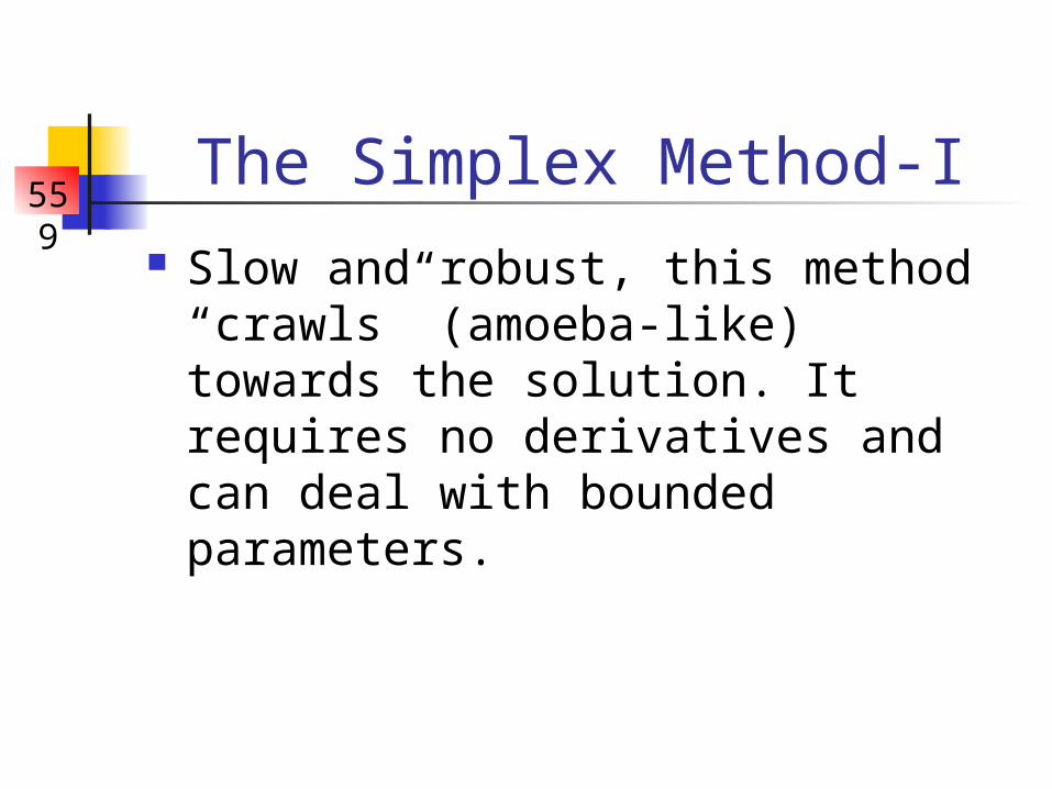
The Simplex Method-I Slow and robust, this method

“crawls” (amoeba-like) towards the solution. It requires no derivatives and can deal with bounded parameters.

559

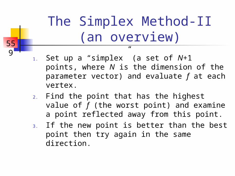
The Simplex Method-II(an overview)

1. Set up a “simplex” (a set of N+1 points, where N is the dimension of the parameter vector) and evaluate f at each vertex.

2. Find the point that has the highest value of f (the worst point) and examine a point reflected away from this point.

3. If the new point is better than the best point then try again in the same direction.

559

The Simplex Method-III(an overview)

4. If the reflected point is worse than the second worst point:

1. replace the worst point if the reflected point is better than the worst point;

2. contract back away from the reflected point;3. if the contracted point is better than the

highest point replace the highest point; and4. if the contracted point is worse that the worst

point contract towards the best point.5. Replace the worst point by the reflected

point.6. Repeat steps 2-5 until the algorithm

converges.

559

parameter 1

pa

ram

ete

r 2

-2 -1 0 1 2 3

-10

12

34

5

parameter 1

pa

ram

ete

r 2

-2 -1 0 1 2 3-1

01

23

45

parameter 1

pa

ram

ete

r 2

-2 -1 0 1 2 3

-10

12

34

5

parameter 1

pa

ram

ete

r 2

-2 -1 0 1 2 3

-10

12

34

5

parameter 1

pa

ram

ete

r 2

-2 -1 0 1 2 3

-10

12

34

5

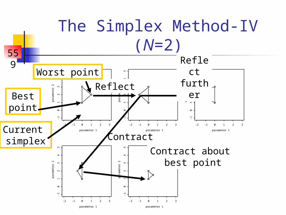
The Simplex Method-IV(N=2)

Current simplex

Reflect

Worst point

Bestpoint

Reflect

further

Contract

Contract about best point

559

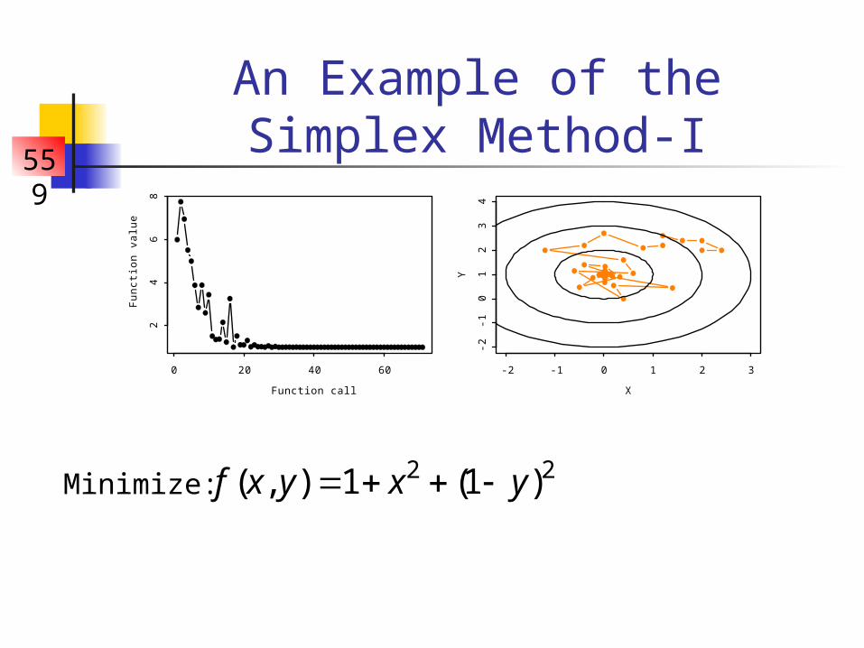
An Example of the Simplex Method-I

Function call

Fu

nct

ion

va

lue

0 20 40 60

24

68

X

Y

-2 -1 0 1 2 3

-2-1

01

23

4Minimize: 2 2( , ) 1 (1 )f x y x y

559

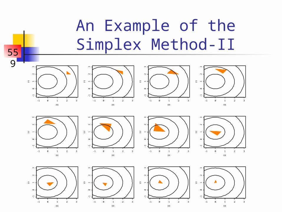
An Example of the Simplex Method-II

XX

YY

-1 0 1 2 3

-10

12

3

XX

YY

-1 0 1 2 3

-10

12

3

XX

YY

-1 0 1 2 3

-10

12

3

XX

YY

-1 0 1 2 3

-10

12

3

XX

YY

-1 0 1 2 3

-10

12

3

XX

YY

-1 0 1 2 3

-10

12

3

XX

YY

-1 0 1 2 3

-10

12

3

XX

YY

-1 0 1 2 3

-10

12

3

XX

YY

-1 0 1 2 3

-10

12

3

XX

YY

-1 0 1 2 3

-10

12

3

XX

YY

-1 0 1 2 3

-10

12

3

XX

YY

-1 0 1 2 3-1

01

23

559

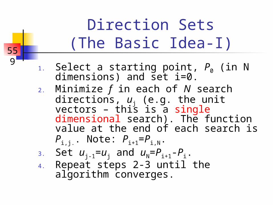
Direction Sets(The Basic Idea-I)

1. Select a starting point, P0 (in N dimensions) and set i=0.

2. Minimize f in each of N search directions, uj (e.g. the unit vectors – this is a single dimensional search). The function value at the end of each search is Pi,j.. Note: Pi+1=Pi,N.

3. Set uj-1=uj and uN=Pi+1-Pi.4. Repeat steps 2-3 until the algorithm

converges.

559

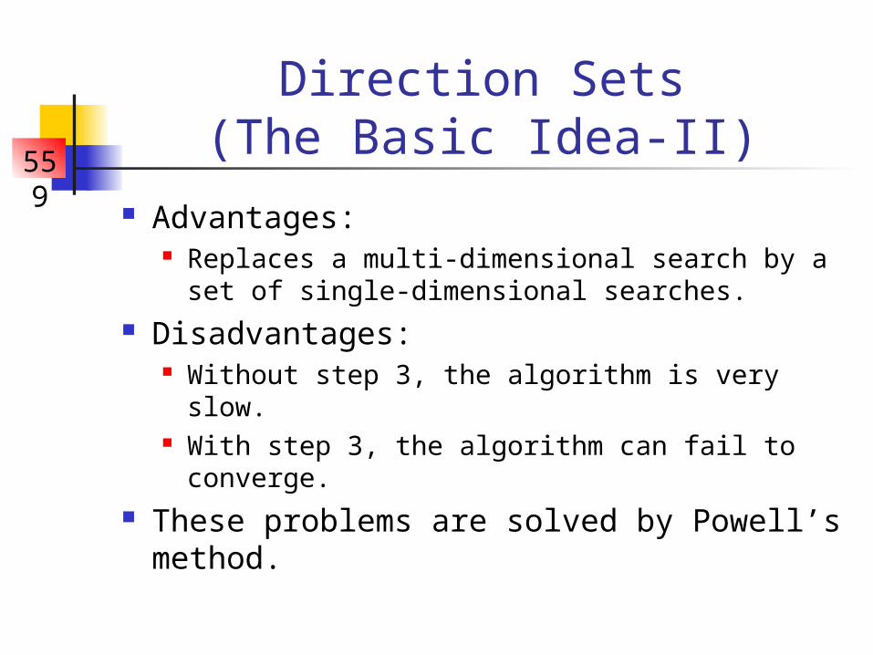
Direction Sets(The Basic Idea-II)

Advantages: Replaces a multi-dimensional search by a

set of single-dimensional searches. Disadvantages:

Without step 3, the algorithm is very slow. With step 3, the algorithm can fail to

converge. These problems are solved by Powell’s

method.

559

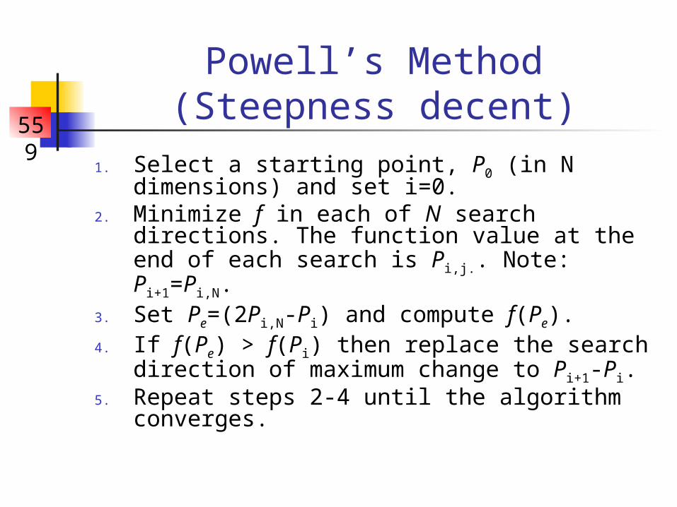
Powell’s Method(Steepness decent)

1. Select a starting point, P0 (in N dimensions) and set i=0.

2. Minimize f in each of N search directions. The function value at the end of each search is Pi,j.. Note: Pi+1=Pi,N.

3. Set Pe=(2Pi,N-Pi) and compute f(Pe).4. If f(Pe) > f(Pi) then replace the search

direction of maximum change to Pi+1-Pi.5. Repeat steps 2-4 until the algorithm

converges.

559

Function call

Fu

nct

ion

va

lue

0 20 40 60 80 100 120

24

68

10

X

Y

-2 -1 0 1 2 3

-2-1

01

23

4

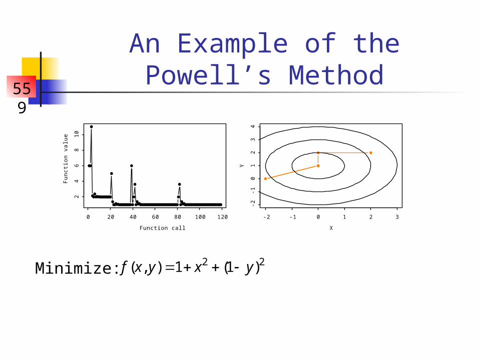
An Example of the Powell’s Method

2 2( , ) 1 (1 )f x y x y Minimize:

559

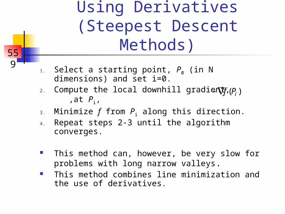
Using Derivatives(Steepest Descent Methods)

1. Select a starting point, P0 (in N dimensions) and set i=0.

2. Compute the local downhill gradient, ,at Pi,

3. Minimize f from Pi along this direction.4. Repeat steps 2-3 until the algorithm converges.

This method can, however, be very slow for problems with long narrow valleys.

This method combines line minimization and the use of derivatives.

( )if P

559

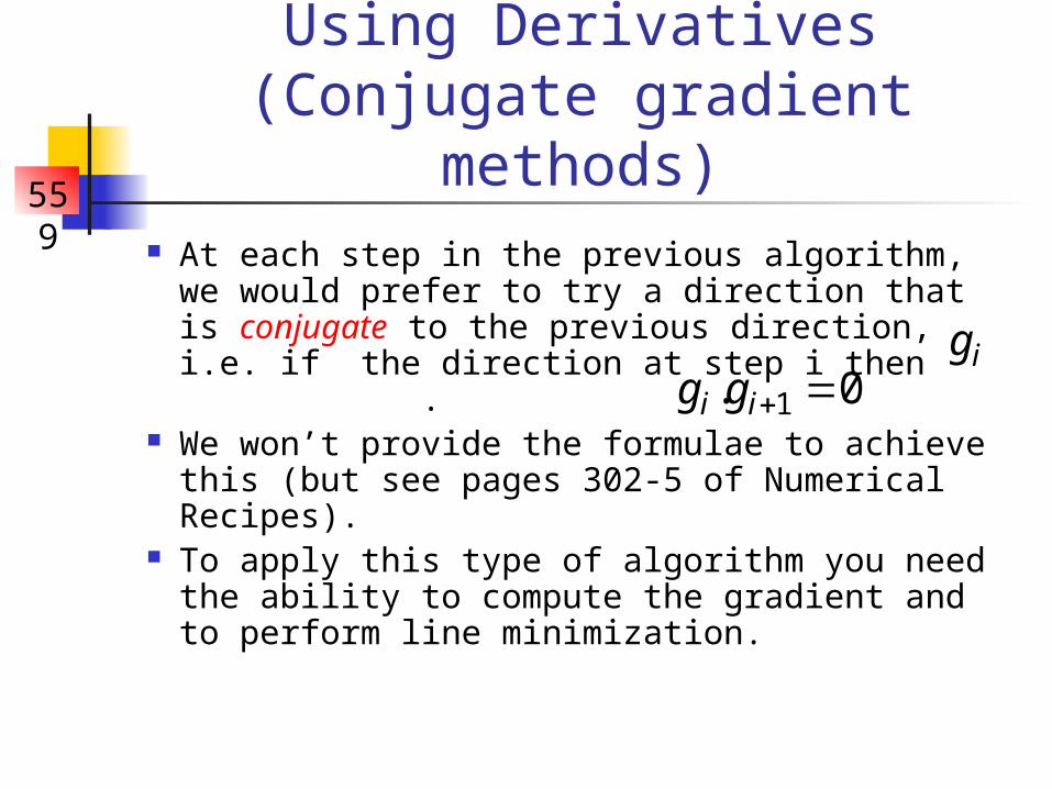
Using Derivatives(Conjugate gradient

methods) At each step in the previous algorithm,

we would prefer to try a direction that is conjugate to the previous direction, i.e. if the direction at step i then .

We won’t provide the formulae to achieve this (but see pages 302-5 of Numerical Recipes).

To apply this type of algorithm you need the ability to compute the gradient and to perform line minimization.

ig1. 0i ig g

559

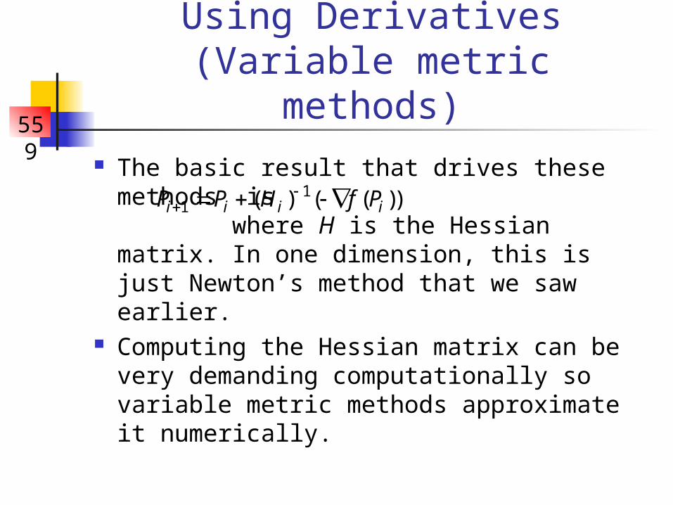
Using Derivatives(Variable metric methods)

The basic result that drives these methods is where H is the Hessian matrix. In one dimension, this is just Newton’s method that we saw earlier.

Computing the Hessian matrix can be very demanding computationally so variable metric methods approximate it numerically.

11 ( ) ( ( ))i i i iP P H f P