MIT OpenCourseWare http://ocw.mit.edu

5.72 Statistical MechanicsSpring 2008

For information about citing these materials or our Terms of Use, visit: http://ocw.mit.edu/terms.

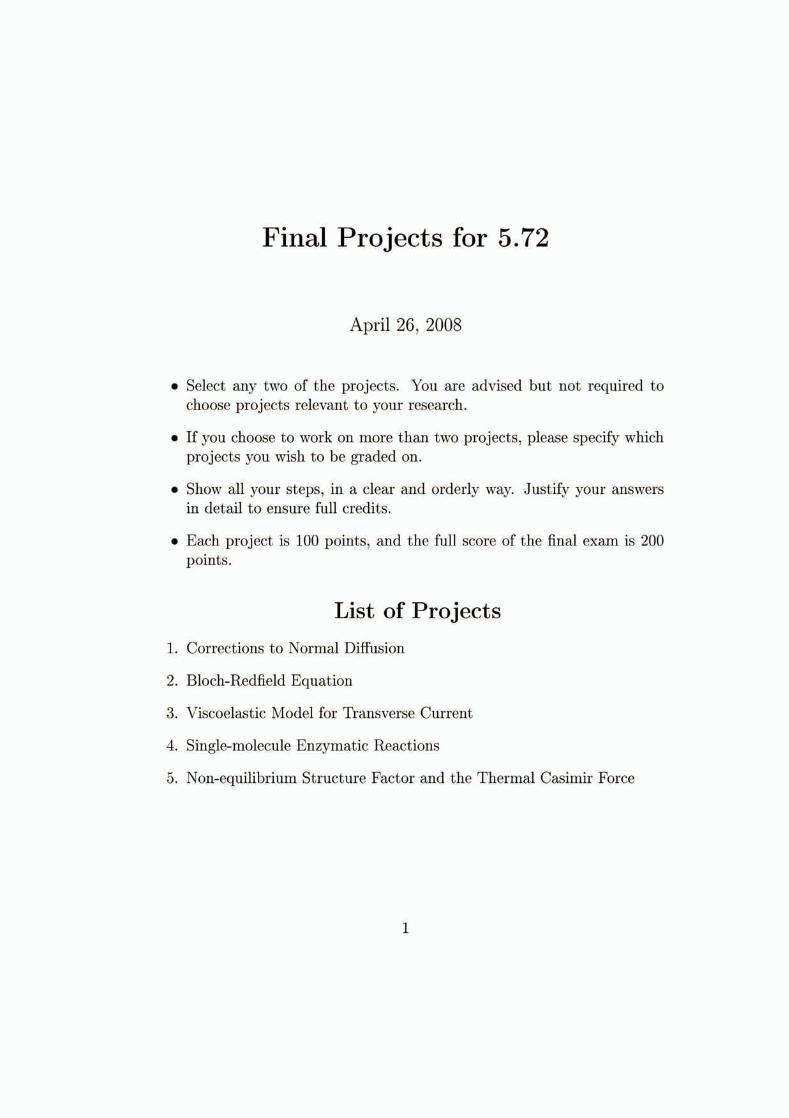
Final Projects for 5.72

April 26, 2008

Select any two of the projects. You are advised but not required to choose projects relevant to your research.

If you choose to work on more than two projects, please specify which projects you wish to be graded on.

Show all your steps, in a clear and orderly way. Justify your answers in detail to ensure full credits.

Each project is 100 points, and the full score of the final exam is 200 points.

List of Projects 1. Corrections to Normal Diffusion

2. Bloch-Redfield Equation

3. Viscoelastic Model for Transverse Current

4. Single-molecule Enzymatic Reactions

5 . Non-equilibrium Structure Factor and the Thermal Casimir Force

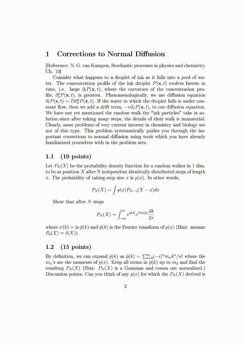
Corrections to Normal Diffusion

[Reference: N. G. van Kampen, Stochastic processes in physics and chemistry, Ch. 101

Consider what happens to a droplet of ink as it falls into a pool of wa- ter. The concentration profile of the ink droplet P(x, t) evolves fastest in time, i.e. large dtP(x,t) , where the curvature of the concentration pro- file, d:P(x, t), is greatest. Phenomenologically, we use diffusion equation dtP(x, t) Dd:P(x, t). If the water in which the droplet falls is under con- stant flow, then we add a drift term, -vd,P(x, t ) ,to our diffusion equation. We have not yet mentioned the random walk the "ink particles" take in so- lution since after taking many steps, the details of their walk is immaterial. Clearly, most problems of very current interest in chemistry and biology are not of this type. This problem systematically guides you through the im- portant corrections to normal diffusion using tools which you have already familiarized yourselves with in the problem sets.

1.1 (10 points)

Let PN(X) be the probability density function for a random walker in 1dim. to be at position X after N independent identically distributed steps of length x. The probability of taking step size x is p(x). In other words,

Show that after N steps

where $(k) = ln$(k) and $(k) is the Fourier transform of p(x) (Hint: assume Po(X) = W ) ) .

1.2 (15 points)

By definition, we can expand @(k) as $(k) = Cr=,(-i)"mnkn/n! where the mn's are the moments of p(x). Keep all terms in p(k) up to mz and find the resulting PN(X) (Hint: PN(X) is a Gaussian and comes out normalized.) Discussion points: Can you think of any p(x) for which the PN(X) derived is

exact? Explain physically what happens if p(x) is, for example, the Lorentz distribution. What does this say about being able to construct P N ( X )for such distributions?

1.3 (5 points)

In continuous time, we can imagine setting time t = N r , where r is the timestep, and define P N ( X )as f i I , (X) = P ( X , t ) . Verify that this P ( X , t ) satisfies the diffusion equation with drift (ml # 0). What diffusion coefficient, Dl and drift coefficients, v, did you use?

1.4 (15 points)

So far, this problem has been a review: we have seen how a delta function initial condition evolves into a Gaussian in free space and that this is indeed consistent with the picture of normal diffusion.

Now let's go back to 1.1where, we had noted, that PN ( X ) = eikXeN$@)@Jrw 2 ~ -

Show that pN(x)= 1 ...)-dke & ~ e ~ ( - i c f i - f c ~ k 2 + $ c ~ ~ +

27r where the c,'s are cumulants of p(x).

Re-scale by letting w = a o l c and z = (X - where the ~ c ~ ) / ( a f l ) standard deviation a = 6.Call this new function #N(z). Show

where Aj = cj/crs',

1.5 (15 points)

Show that

where H, are the Hermite polynomials. The expansion above is called the Gram-Charlier expansion. Discussion point: Why is this approx. only valid for small z? Qualitatively, how does this correction affect the spread of our ink droplet in continuous time?

1.6 (10 points)

Clearly the approximate q5N (2) just derived no longer satisfies the normal diffusion equation. It must satisfy another diffusion-type equation, maybe not exactly, but at least to the right order. By finding this equation, we derive the Kramers-Moyall expansion.

Recall that (X) = J p(x)PN(X - x)dx. Expand the right hand side of this equation around x and show

Show that in continuous time we can expand the left hand side to obtain

1.7 (10 points)

From 1.6 we have

Taking a time derivative of the above returns

We can substitute the first equation of 1.7 into the above in order to ex- press a;P(X,t) in terms of x derivatives of P(X, t) only plus corrections 0 (~ ,3P(X,t) , a,3P(X, t)).

Use this result to verify that, to leading order, we obtain the normal diffusion equation

1.8 (20 points)

Repeat 1.7 by keeping O(a2 P(X,t), @P(X, t)) . Find the leading corrections to normal diffusion equation. This equation should be one where dtP(X, t) is set equal to x derivatives of P(X, t). Physically interpret the effect of this term on normal diffusion. (Hint: The result is very simple and should be obvious from 1.5 once com- puted).

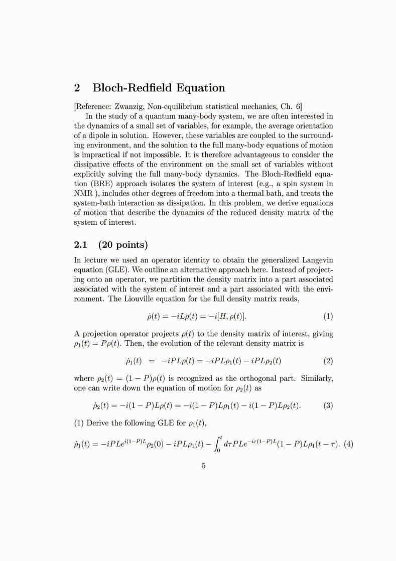
Bloch-Redfield Equation [Reference: Zwanzig, Non-equilibrium statistical mechanics, Ch. 61

In the study of a quantum many-body system, we are often interested in the dynamics of a small set of variables, for example, the average orientation of a dipole in solution. However, these variables are coupled to the surround- ing environment, and the solution to the full many-body equations of motion is impractical if not impossible. It is therefore advantageous to consider the dissipative effects of the environment on the small set of variables without explicitly solving the full many-body dynamics. The Bloch-Redfield equa- tion (BRE) approach isolates the system of interest (e.g., a spin system in NMR ), includes other degrees of freedom into a thermal bath, and treats the system-bath interaction as dissipation. In this problem, we derive equations of motion that describe the dynamics of the reduced density matrix of the system of interest.

2.1 (20 points)

In lecture we used an operator identity to obtain the generalized Langevin equation (GLE). We outline an alternative approach here. Instead of project- ing onto an operator, we partition the density matrix into a part associated associated with the system of interest and a part associated with the envi- ronment. The Liouville equation for the full density matrix reads,

A projection operator projects p(t) to the density matrix of interest, giving pl(t) = Pp(t). Then, the evolution of the relevant density matrix is

pl(t) = -iPLp(t) = -iPLpl (t) - iPLp2(t)

where p2(t) = (1 - P)p(t) is recognized as the orthogonal part. Similarly, one can write down the equation of motion for p2(t) as

(1)Derive the following GLE for pl (t) ,

[Hint: Use equation (3) to solve pz(t) in terms of pl (t) and pz (0), and then substitute the expression for pz(t)into equation (2).]

(2) Identify the frequency, the dissipation, and the fluctuation t e r n . When will the noise be identically zero?

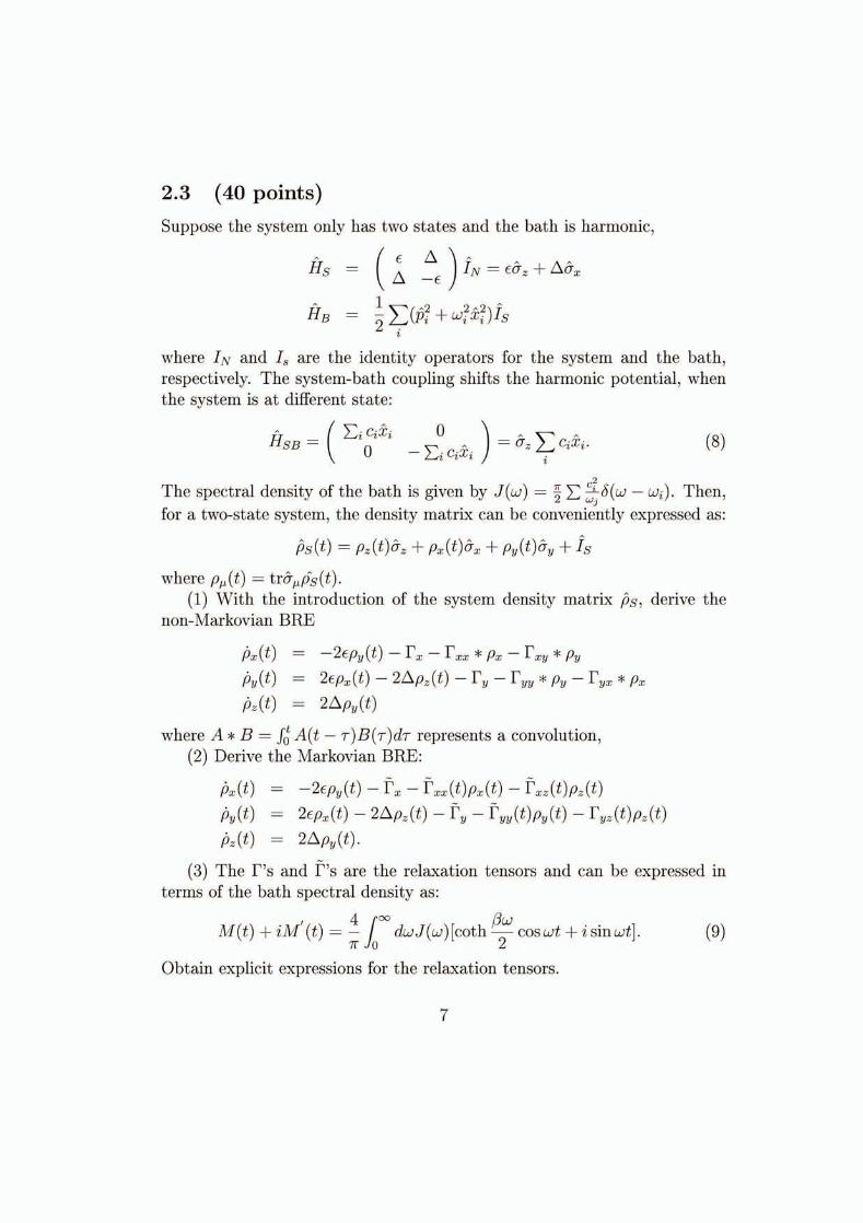
2.2 (40 points)

The Bloch-Redfield equation (BRB) describes the dynamics of the reduced density matrix, and can be obtained from the GLE. Suppose the total Hamil- tonian is written as:

H = H s + H g + H s ~

where Hs and Hg operate on the system and bath degrees of freedom, re- spectively, and HSB operates on both system and bath. For simplicity, we assume that the initial density is in a product state, p(0) = p~ (8r ps(0), and trBHsBp~= 0. TO use the GLE derived above, we define the projection o p

-ORBerator as P = p~ @ trg, where p~ = +is the equilibrium distribution of the bath and trB denotes a trace over the bath degrees of freedom. The projection operator defmes the reduced density matrix,

(1)Show that the noise in the GLE is zero. (2) Derive the explicit form of the GLE

and obtain the memory kernel in the form of K(t )= trB{~sBe-iL(l-P)t~SBPB).

Here, the Liouville operator is written as L = Ls + LB + LSB. (3) Under the approximation K(t) = trs{~sBe-i(Ls'LB)t~SBPB1, derive

the non-Markovian BRE,

(4) Applying an additional approximation in equation (7), ps(t - T ) = eZs7ps(t), derive a Markovian BRE. Is the Markovian B W correct to second order in HSB?

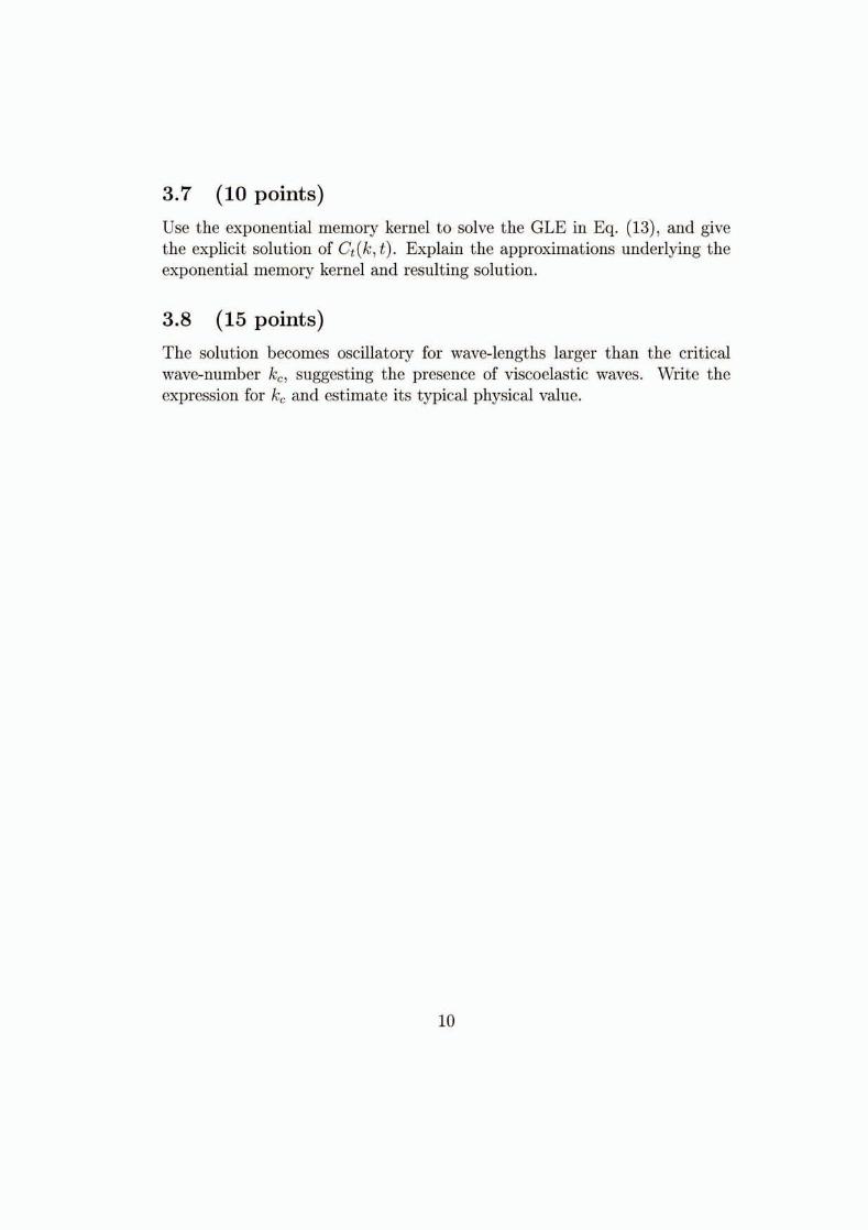
2.3 (40 points)

Suppose the system only has two states and the bath is harmonic,

where IN and I, are the identity operators for the system and the bath, respectively. The system-bath coupling shifts the harmonic potential, when the system is at different state:

The spectral density of the bath is given by J ( w ) = C $(w -w,). Then, for a two-state system, the density matrix can be conveniently expressed as:

6s(t)= + fspz ( t ) k z +px (t)+x + P Y ( ~ ) ~ Y

where p,(t) = tr6,Fs(t). (1)With the introduction of the system density matrix bs, derive the

non-Markovian BRE

where A * B = $A(t r )B ( T ) ~ T- represents a convolution, (2 ) Derive the Markovian BRE:

(3) The r 's and f ' s are the relaxation tensors and can be expressed in terms of the bath spectral density as:

4 O 0 PwM ( t ) + i ~ ( t) -1 dw J ( w ) [coth1cos wt + i sin wt] .' =

7T 0

Obtain explicit expressions for the relaxation tensors.

Viscoelastic Model for Transverse Current

[Reference: U. Balucani and M. Zoppi, Dynamics of the liquid state, Sec. 3.4.2 and Sec. 6.2.21

Molecular hydrodynamics provides a bridge between long-time hydro- dynamics and short-time molecule dynamics. As an example, we use the transverse current Jt(k, t ) = xg,xj exp(ikzj) to illustrate the viscoelastic approximation in molecule hydrodynamics. In the long-time long-wavelengt h hydrodynamics limit, the transverse current dissipates through diffusion with a coefficient proportional to shear viscosity q~.In the opposite limit, liquids behave like solids, which support mechanical waves characterized by high- frequency shear modulus G(k). Viscoelastic theory interpolates between the two limits and predicts the dynamic slow-down of transverse current fluctu- ations as a function of wave-number k.

3.1 (15 points)

The transverse current correlation function is defined as Ct(k, t) = 5(Jt(k,t )1 Jt(k,0)), where N is the particle number. The short-time expansion of Ct(k, t) reads

Show v; = kT/m and w: = k2cz(k) with the speed of sound

Here, g ( r ) is the pairwise correlation function and U(r) is the pairwise inter- action potential.

3.2 (15 points)

For an ideal gas sample, the transverse current correlation function reads

Ct (k, t )= (vieihzt)= ui exp[- ( ~ o t ) ~ / 2 ]

with WE = uik2. Verify that the free particle expression is consistent with short-time expansion in Eq. (10) and estimate the length-scale when collisions become relevant.

3.3 (15points)

Use the generalized Langevin equation (GLE) derived in class to obtain

where v(k, t) is the shear viscosity function or the memory function. In writing Eq. (13), you need to justify that the memory kernel in GLE is proportional to k2, i.e., M(k, t) = k2v(k, t), and give an formal expression for v(k, t ) .

3.4 (10points)

At short time, the GLE in Eq. (13) takes the form of

which supports a propagating shear elastic wave. Write the functional form of the propagating waves and show that the speed of the elastic wave is v(k, 0) = <(k) = G(k)/pm

3.5 (10points)

At long time, the GLE is simplified with the Markovian approximation and takes the hydrodynamic solution,

G(k , t) +k2vCt(k, t) = 0

Show the long-wavelength limit of the shear viscosity function J,OO v(0, t)dt =

v = qlpm and write the fluctuation spectrum of the transverse current.

3.6 (10points)

The viscoelastic model assumes an exponential memory kernel v(k7 t) =

v(k, o ) ~ - ~ ' ~ M ,where the Maxwell relaxation time TM defines the time-scale separating the short-time and long-time behavior. Use the short-time and long-time limits to obtain the value of the Maxwell time

and explain its physical meaning.

3.7 (10 points)

Use the exponential memory kernel to solve the GLE in Eq. (13), and give the explicit solution of Ct( k ,t ) . Explain the approximations underlying the exponential memory kernel and resulting solution.

3.8 (15 points)

The solution becomes oscillatory for wave-lengths larger than the critical wave-number Ic,, suggesting the presence of viscoelastic waves. Write the expression for kc and estimate its typical physical value.

Single-molecule Enzymatic Reactions [Reference: See manuscript 'Generic schemes of single molecule kinetics: Self- consistent pathway solutions to renew processes']

In class, we introduced a simple method, 'pathway summation', to cal- culate the evolution of probability in a discrete Markov chain . We will now generalize the method to single-molecule reaction processes and predict the first-passage time distribution function of enzymatic turnover reactions. The basic idea is to calculate the joint probability of transitions along each path- way leading to the product state and sum up the probabilities of all possible pathways. The pathway summation method is intuitive and has recently been applied to single molecule reactions, molecular motors, and photon statistics.

4.1 (10 points)

A fundamental chemical reaction follows single exponential decay, Q(t) =

ke-", where Q(t) is the probability distribution function (PDF) of decay. Evaluate the 1-th moment of the first passage time (tm) = JQ(t)tmdt and confirm

where Q(s) = J e-stQ(t)dt is the Laplace transform and s is the Laplace variable.

4.2 (10 points)

Consider a two-step sequential reaction, A1 +A2 -+ A3, with rate constants k12 and k23, respectively. The distribution of the first passage time from Al to A3 is

or, in Laplace space, QI3(s) = Q12(~)Q23(~) .Write an explicit expression for QI3(t) and calculate the mean first passage time (t). Explain the initial value of the calculated QI3(t) is zero, QI3(0) = 0.

4.3 (10 points)

We now generalize the above argument to a chain reaction with multiple steps, Al +A2.- +An-1 +A,. The PDF of the first passage time reads

where n is the final state. Use the above expression to obtain an expression for the mean first passage time (t).

4.4 (15 points)

A sequence of chemical reactions can achieve remarkable timing, giving rise to the notion of 'biological clock'. To demonstrate this effect, consider a sequence of n reactions with identical rate constant kl = k l . . . = k, =

nlc. Calculate the distribution Ql,,(t),mean first passage time ( t ) ,and the variance (6t2)= ( ( t- ( t ) )2) .Plot Ql,,(t) as a function of time for n=l, 2, and 10, respectively, and explain the change in Q(t)as n increases.

4.5 (10 points)

Consider decay from state 0 to state 1with rate kol and to state 2 with rate kO2.We assign the transition PDF7s of the branching reaction as Qol(t)=

lcO1e-ht and Q02(t)= h2e-lcot with ko = kol + kO2the depletion rate from state 0. Explain the above result and generalize it to decay from state 0 to n different states.

4.6 (15 points)

The Michaelis-Menten mechanism of enzymatic reactions is given by

which consists of three states: state 1,free substrates and enzyme; state 2, substrate-enzyme complex; and state 3, product. With the constant sub- strate concentration [S], the stationary-state population of state 2 can be determined from

where kl = ky[S] is the substrate binding rate, k-1 is the dissociation rate, and k2 is the catalytic rate. For a single enzyme, its probability is conserved, giving [E]+[ES]=l. Derive the stationary-state population

kl[ES]= kl +k-1 + k2

and the Michaelis-Menten rate

with the Michaelis constant kM = (k-1 + k2)/ky.

4.7 (20 points)

We now apply the pathway summation technique to the Michaelis-Menten scheme in Eq. (20). Starting from state 1, a substrate [S] binds with the enzyme [El to form a substrate-enzyme complex [ES], i.e., state 2, which can branch to form a product [PI or return to the state 1. Following the pathway, we obtain the PDF of the turnover time by solving self-consistently

where the two terms in the bracket represents the two decay channels from state 2. Solution to the self-consistent equation in Eq. (24) yields

Expand the denominator in the above expression, draw the pathway associ- ated with each term in the expansion, and explain the self-consistent solution in Eq. (25).

4.8 (10 points)

The PDF7s associated with the three reaction steps are specified by rate con- stants as Q12(t)= kle-klt, Q21(t) = k-le-(k-lSkz)t, and Q23(t) = k2e-(k-1Skz)t, with kl = ky [S]. Use Eq. (25) to derive the mean first passage time and con- firm the Michaelis-Menten expression in Eq. (23), derived earlier using the st ationary-state approach.

Non-equilibrium Structure Factor and the Ther-mal Casimir Force

[Problem is self-contained. If interested in learning more, see R. Brito et al., PRE 76, 011113(2007)].

Consider a fluid at equilibrium: the structure factor for such a fluid re- veals that density fluctuations are delta correlated in space and time. Many relevant systems currently under study, especially in biology, are not at equi- librium. In non-equilibrium(non-eq.) systems, long-range correlations in the density fluctuations may arise. Suppose two solid parallel planes are placed in the non-equilibrium fluid with fluid both between and outside these planes. The planes can be thought of as cell membranes through which no fluid passes. The fluid exerts a force onto those planes by virtue of not being at equilibrium! This amazing force, the so-called thermal Casimir force which is under current intense investigation, arises because the planes break the non-equilibrium. fluid's long-range correlations. This problem systemati- cally guides you through a simple calculation of the thermal Casimir force using notions which you have already been familiarized with in your problem sets.

Suppose the fluid density fluctuations satisfy

where 4 = n - no is the deviation from the homogeneous fluid denisty, no, D the diffusion coeff., X the relaxation rate and the multi-component t1and single component J2 are the fluctuations in the diffusive flux and the reaction rate, respectively.

Take d) ) = r16,6(r - r')6(t -d)

5.1 (15 points)

We begin with the problem in free space(no boundaries) and define the Fourier transform &(t) = J dVe-""4(r, t) and similarly for &(r, t) and G(r ,t).

(;, (h i ( r , t ) h j

Show

and

(in,Z(t)i,.t(t')) = v4,-nr26(t - t))

5.2 (15points)

Using part 5.1, show that the static(t -+ m) structure factor S(k) = % + r 2 0& where ko = and I'= I'2-rlX/D.Compute the Fourier trans- form of S(k) to find G(r). Physically interpret the form for G(r). (Hint 1: ( 4 k 4 q ) = VS(k)&,-,.) (Hint 2: You may compute G(r) on Mathemtica if you prefer.)

5.3 (10points)

The static structure factor from part 5.2 can be re-written as S(k) = 2 + S*(k) where S*(k) is the non-eq. part. At equilibrium, when the fluctuation- dissipation theorem is satisfied, (Ad,) = VQ,-,kT. F'rom this, find the equilibrium I'I and r2. Discussion point: What is difference between the non-equ. S(k) and the equilibrium S(k)? Repeat discussion for G(r).

5.4 (20points)

Now that we have seen how long-range correlations arise when the fluc.- diss. theorem is not satisfied, let's change the fluctuation spectrum, S(k), by introducing boundaries in the medium containing our fluid.

Consider adding a plate in the x = 0 plane and another in the x = L plane with nonflux boundary conditions across them. The volume between the plates is V = L x L, x L, where L,, L, + m since the y and x directions remain completely free. The volume between the plates is called Region I. The volume outside the plates is called Region 11. There are therefore 2 Regions 11,one to the left and another to the right of Region I. The volume of each Region I1 is V = X x L, x L, where X = L, -L and L,, L,, L, -+ m.

For these boundary conditions, the density fluctuations are expanded as follows

+(r,t) = V-' C Jk (t)cos(k,x)e"~Y eikzz ks,ky ,k*

where kx = =nx/X, Icy = nny/Ly, k, = nnz/Lz and n, = 0,1,2... while ny l nz = .. - 1,0, 1,...

Show that (ik,l(t)i,l(t '))= yksV$,-,r,s(t - t')

where ykx = 1/2 if IC,^=O and 7 k X = 1otherwise. Also, show that (#k#,) = VykzS(k)Gk,-, and that the real-space non-eq.

density fluctuations satisfy

where the prime means that the kz = 0 term has a factor 112 and q = k/ko.

5.5 (15points)

Technically, the (#(r,t)2) as written at the end of 5.4 diverges as q + m. However, we are only interested in looking at the difference between the fluc- tuations (+(r, t)2) in Region I and Region 11. While both quantities diverge, the difference between these fluctuations is finite and tells us something about the applied force on the plate.

These divergences are typical of ALL Casirnir force calculations and ex- plaining their existence is beyond the scope of this problem, e.g. in quantum Casimir force calculations they arise because of the infinite vacuum zero-point energy.

For now, we "patch-up" our problem by introducing a regularizing func- tion 1/(1+ e2q2) which tends to 1as e +O+. In other words,

We will be interested in (+(r,t ) 2 )near x = L or x = 0 where the cosine term in the above is 1.

Show that in Region I, where the q, and q, sums can be turned into integrals,

and that in region I1

(HINT: you can use Mathematica).

5.6 (25 points)

Suppose that the average pressure in regions I and I1 is a function of n alone, (p) = (p(n)). Expand the pressure around the uniform density to second order. Express the difference in pressure evaluated to second order in region I and I1 in terms of ($(r ,t)2)I I and ($(r ,t)2)1. This net differential force per unit area FIA, i.e. the difference in pressure, is the thermal Casimir force.

Finally, show that

where Fo = rko(aip(no))ll67rD and I = koL,. Discussion points: How does the force, FIA, scale in the short distance regime? How does it scale in the long distance regime? Can you physically interpret the scalings and the sign of the force? Should the force really diverge at short distances as the theory predicts?