5960 ieee transactions on information...

5960 IEEE TRANSACTIONS ON INFORMATION THEORY, VOL. 57, NO. 9, SEPTEMBER 2011

Efficient Implementation of LinearProgramming Decoding

Mohammad H. Taghavi, Member, IEEE, Amin Shokrollahi, Fellow, IEEE, and Paul H. Siegel, Fellow, IEEE

Abstract—While linear programming (LP) decoding providesmore flexibility for finite-length performance analysis than it-erative message-passing (IMP) decoding, it is computationallymore complex to implement in its original form, due to boththe large size of the relaxed LP problem and the inefficiency ofusing general-purpose LP solvers. This paper explores ideas forfast LP decoding of low-density parity-check (LDPC) codes. Bymodifying the previously reported Adaptive LP decoding schemeto allow removal of unnecessary constraints, we first prove that LPdecoding can be performed by solving a number of LP problemsthat each contains at most one linear constraint derived fromeach of the parity-check constraints. By exploiting this property,we study a sparse interior-point implementation for solving thissequence of linear programs. Since the most complex part ofeach iteration of the interior-point algorithm is the solution of a(usually ill-conditioned) system of linear equations for finding thestep direction, we propose a preconditioning algorithm to facilitatesolving such systems iteratively. The proposed preconditioningalgorithm is similar to the encoding procedure of LDPC codes,and we demonstrate its effectiveness via both analytical methodsand computer simulation results.

Index Terms—Adaptive linear programming (LP) decoding,conjugate-gradient method, interior-point methods, low-densityparity-check (LDPC) codes, preconditioning.

I. INTRODUCTION

L OW-DENSITY parity-check (LDPC) codes [1] arebecoming one of the dominant means of error-control

coding in the transmission and storage of digital information.By combining randomness and sparsity, LDPC codes with largeblock lengths can correct errors using iterative message-passing(IMP) algorithms at coding rates that are closer to the capacitythan any other class of practical codes [2]. While the perfor-mance of IMP decoders for the asymptotic case of infinitelengths is studied extensively using probabilistic methods

Manuscript received December 12, 2008; revised March 09, 2011; acceptedApril 12, 2011. Date of current version August 31, 2011. Part of the researchon this paper was done when M. H. Taghavi was visiting EPFL in the summerof 2007. The material in this paper was presented in part at the 3rd AnnualInformation Theory and Applications Workshop (ITA’08), La Jolla, CA, January2008, and in part at the 46th Annual Allerton Conference on Communication,Control, and Computing, Monticello, IL, September 2008.

M. H. Taghavi was with the Electrical and Computer Engineering Depart-ment, University of California, San Diego, La Jolla, CA 92093-0407 USA. He isnow with Qualcomm, Inc., San Diego, CA 92121 USA (e-mail: [email protected]).

A. Shokrollahi is with the School of Basic Sciences and School of Com-puter Science and Communications, Ecole Polytechnique Fédérale de Lausanne(EPFL), 1015 Lausanne, Switzerland (e-mail: [email protected]).

P. H. Siegel is with the Electrical and Computer Engineering Departmentand the Center for Magnetic Recording Research, University of California, SanDiego, La Jolla, CA 92093-0401 USA (e-mail: [email protected]).

Communicated by I. Sason, Associate Editor for Coding Theory.Digital Object Identifier 10.1109/TIT.2011.2161920

such as density evolution [3], the finite-length behavior ofthese algorithms, especially their error floors, are still not wellcharacterized.

Linear programming (LP) decoding was proposed byFeldman et al. [4] as an alternative to IMP decoding ofLDPC and turbo-like codes. LP decoding approximates themaximum-likelihood (ML) decoding problem by a linear op-timization problem via a relaxation of each of the finite-fieldparity-check constraints of the ML decoding into a numberof linear constraints. Many observations suggest similaritiesbetween the performance of LP and IMP decoding methods[4]–[6]. In fact, the sum-product message-passing algorithmcan be interpreted as a minimization of a nonlinear function,known as Bethe free energy, over the same feasible region asLP decoding [7], [8].

Due to its geometric structure, LP decoding seems to be moreamenable than IMP decoding to finite-length analysis. In par-ticular, the finite-length behavior of LP decoding can be com-pletely characterized in terms of pseudocodewords, which arethe vertices of the feasible space of the corresponding linearprogram. Another characteristic of LP decoding—the ML cer-tificate property—is that its failure to find an ML codeword isalways detectable. More specifically, the decoder always giveseither an ML codeword or a nonintegral pseudocodeword as thesolution. On the other hand, the main disadvantage of LP de-coding is its higher complexity compared to IMP decoding.

In order to make linear programming (LP) decoding practical,it is necessary to find efficient implementations that make itstime-complexity comparable to those of the message-passingalgorithms. A conventional implementation of LP decoding ishighly complex due to two main factors: (1) the large size ofthe LP problem formed by relaxation, and (2) the inability ofgeneral-purpose LP solvers to solve the LP efficiently by takingadvantage of the properties of the decoding problem.

The standard formulation of LP decoding [4] has a size thatgrows very rapidly with the density of the Tanner graph repre-sentation of the code. Adaptive LP (ALP) decoding was pro-posed in [9] to address this problem, reducing LP decoding tosolving a sequence of much smaller LP problems. The size ofthese LP problems has been observed in practice to be indepen-dent of the degree distribution, and more specifically, a smallfactor (less than two) times the number of parity checks. How-ever, this observation has not been analytically explained.

More recently, an equivalent formulation of the LP decodingproblem was proposed in [11] and [12], with a problem sizegrowing linearly with both the code length and the maximumcheck node degrees. While this formulation requires solvingonly one LP, the overall complexity of this method in practiceremains substantially higher than that of ALP decoding.

0018-9448/$26.00 © 2011 IEEE

TAGHAVI et al.: EFFICIENT IMPLEMENTATION OF LINEAR PROGRAMMING DECODING 5961

In this paper, we take some steps toward designing efficientLP solvers for LP decoding that exploit the inherent sparsity andstructure of this particular class of problems. Our approach isbased on a sparse implementation of interior-point algorithms.In an independent work, Vontobel studied the implementationand convergence of interior-point methods for LP decoding andmentioned a number of potential approaches to reduce its com-plexity [13]. It is also worth noting that a different line of workin this direction has been to apply iterative methods based onmessage-passing, instead of general LP solvers, to perform theoptimization for LP decoding; e.g., see [8] and [14].

The contributions of this paper are divided into two mainparts; the results given in the first part lay the foundation andprovide motivation for the techniques proposed in the secondpart. In the first part of our contributions, we first propose twomodified versions of ALP decoding. The main idea behindthese modifications is to adaptively remove a number of con-straints at each iteration of ALP decoding, while adding newconstraints to the problem. We prove a number of propertiesof these algorithms, which facilitate the design of a low-com-plexity LP solver. In particular, we show that the modified ALPdecoders have the single-constraint property, which meansthat they perform LP decoding by solving a series of linearprograms that each contain at most one linear constraint fromeach parity check. An important consequence of this propertyis that the constraint matrices of the linear programs that aresolved have a structure similar, in terms of the locations of theirnonzero entries, to that of the parity-check matrix. This andother analytical results presented in the first part are exploitedlater in the paper to develop a more efficient interior-point LPsolver.

In the second part, we focus on the most complex part ofeach iteration of the interior-point algorithm, which is solvinga system of linear equations to compute the Newton step. Sincethese linear systems become ill-conditioned as the interior-pointalgorithm approaches the solution, iterative methods that areoften used for solving sparse systems, such as the conjugate-gra-dient (CG) method, perform poorly in the later iterations of theoptimization. To address this problem, we propose a criterionfor designing preconditioners that take advantage of the prop-erties of LP decoding, along with a number of greedy algo-rithms to search for such preconditioners. The proposed pre-conditioning algorithms have similarities to the encoding pro-cedure of LDPC codes, and we demonstrate their effectivenessvia both analytical methods and computer simulation results. Itis important to note that, while the preconditioning techniquesproposed are motivated by the structure of the (modified) ALPdecoders, the applications of these techniques are not limited tosolving LPs given by ALP decoders, and they can be applied tovarious classes of sparse LP problems, including nonadaptiveLP decoding.

The rest of this paper is organized as follows. In Section II,we review linear codes, LP decoding, and ALP decoding. InSection III, we propose some modifications to ALP decoding,and demonstrate a number of properties of ALP decoding and itsvariations. In Section IV, we review a class of the interior-pointlinear programming methods, as well as the preconditioned con-jugate gradient (PCG) method for solving linear systems, with

an emphasis on sparse implementation. In Section V, we intro-duce the proposed preconditioning algorithms to improve thePCG method for LP decoding. Some theoretical analysis andcomputer simulation results are presented in Section VI, andsome concluding remarks are given in Section VII.

II. LP DECODING

A. Notation

Throughout the paper, we denote scalars and column vectorsby lower-case letters , matrices by upper-case letters ,and sets by calligraphic upper-case letters . We write theth element of a vector and the th element of a matrix

as and , respectively. Furthermore, whenever one sideof an equation or inequality is a vector and the other side is aconstant such as 0, the latter is interpreted as a vector of thecorresponding length with all its elements equal to that constant.The cardinality (size) of a finite set is shown by . Thesupport set (or briefly, support) of a vector of length is theset of locations such that . Similarly,the fractional support of a vector is the set of locations

such that .A binary linear code of block length is a subspace of

. This subspace can be defined as the null space (kernel)of a parity-check matrix . In other words

(1)

Hence, each row of corresponds to a binary parity-check con-straint. The design rate of this code is defined as . Inthis paper, we assume that has full row rank, in which casethe design rate is the same as the rate of the code.

Given the parity-check matrix, , the code can alsobe described by a Tanner graph. The Tanner graph is a bi-partite graph containing variable nodes (corresponding to thecolumns of ) and check nodes (corresponding to the rowsof ). We denote by the set of (indices of) vari-able nodes, and by the set of (indices of) checknodes. Variable node is connected to check node via an edgein the Tanner graph iff .

The neighborhood of a check (variable) node is theset of variable (check) nodes it is directly connected to via anedge, i.e., the support set of the th row (column) of . Thedegree of a node is the cardinality of its neighborhood. Let

be a subset of the variable nodes. We call a stoppingset if there is no check node in the graph that has exactly oneneighbor in . Stopping sets characterize the termination of abelief propagation erasure decoder.

Each code can be equivalently represented by many differentparity-check matrices and Tanner graphs. However, it is impor-tant to note that the performance of suboptimal decoders, such asmessage-passing or LP decoding, may depend on the particularchoice of and . A low-density parity-check (LDPC) codeis a linear code which has at least one sparse Tanner graph rep-resentation, where, roughly speaking, the average variable nodeand check node degrees are “small” with respect to or .


A linear program (LP)1 of dimension is an optimiza-tion problem with a linear objective function and a feasible set(space) described by a number of linear constraints (inequalitiesor equations) in terms of real-valued variables. Each linearconstraint in the LP defines a hyperplane in -dimensionalspace. If the solution to an LP is bounded and unique, then it isat a vertex of the feasible space, on the intersection of at least

such hyperplanes. Conversely, for any vertex of the feasiblespace of an LP, there exists a choice of the coefficients of theobjective function such that is the unique solution to the LP.

B. LP Relaxation of Maximum-Likelihood Decoding

Consider a binary linear code of length . If a codewordis transmitted through a memoryless binary-input output-

symmetric (MBIOS) channel, the ML codeword given thereceived vector is the codeword that maximizes thelikelihood of observing , i.e.,

(2)

For binary codes, this problem can be rewritten as the equivalentoptimization problem

(3)

where is the vector of log-likelihood ratios (LLR) defined as

(4)

The ML decoding problem (3) is an optimization with a linearobjective function in the real domain, but with constraints thatare nonlinear in the real space (although, linear in ). It isdesirable to replace these constraints by a number of linear con-straints, such that decoding can be performed using linear pro-gramming. The feasible space of the desired LP would be theconvex hull of all the codewords in , which is called the code-word polytope. Since a global minimum occurs at one of the ver-tices of the polytope, using this feasible space makes the set ofpotential (unique) solutions to the LP identical to the set of code-words in . Unfortunately, the number of constraints needed forthis LP representation grows exponentially with the code length,therefore making this approach impractical. As an approxima-tion to ML decoding, Feldman et al. proposed a relaxed versionof this problem by first considering the convex hull of the localcodewords defined by each row of the parity-check matrix, andthen intersecting them to obtain what is known as the funda-mental polytope, [6].

To describe the (projected) fundamental polytope, linear con-straints are derived from a parity-check matrix as follows. Foreach row of the parity-check matrix, i.e., eachcheck node, the LP formulation includes the constraints

(5)

1Throughout the paper, we abbreviate the terms “linear program” and “linearprogramming” both as “LP.”

which can be written in the equivalent form

(6)

We refer to the constraints of this form as parity inequalities.If the variables are zeroes and ones, these constraints willbe equivalent to the original binary parity-check constraints. Tosee this, note that if is a subset of , with odd, and thecorresponding parity inequality fails to hold, then all variablenodes in must have the value 1, while those in musthave the value 0. This implies that the corresponding vectordoes not satisfy parity check . Conversely, if parity check failsto hold, there must be a subset of variable nodes ofodd size such that all nodes in have the value 1 and all thosein have the value 0. Clearly, the corresponding parityinequality would be violated. Now, given this equivalence, werelax the LP problem by replacing each binary constraint,

, by a box constraint, . LP decoding can thenbe written as

(7)

Lemma 1 ([4], Originally by [17]): For any check node , theset of parity inequalities (5) defines the convex hull of allassignments of the variables with indices in that satisfythe th binary parity-check constraint.

Since the convex hull of a set of vectors in is a subsetof , the set of parity inequalities for each check node au-tomatically restrict all the involved variables to the interval [0,1]. Hence, we obtain the following corollary:

Corollary 1: In the formulation of LP decoding above, thebox constraints for variables that are involved in at least oneparity-check constraint are redundant.

The fundamental polytope has a number of integral (bi-nary-valued) and nonintegral (fractional-valued) vertices. Theintegral vertices, which satisfy all the parity-check equationsas shown before, exactly correspond to the codewords of .Therefore, the LP relaxation has the ML certificate property,i.e., whenever LP decoding gives an integral solution, it isguaranteed to be an ML codeword. On the other hand, if LPdecoding gives as the solution one of the nonintegral vertices,which are known as pseudocodewords, the decoder declares afailure.

C. Adaptive Linear Programming Decoding

In the original formulation of Feldman et al. for LP decoding[4], the number of parity inequalities for each check node of de-gree is equal to the number of odd-sized subsets of its neigh-borhood, which is equal to . In the same article, anotherformulation of the problem is presented with constraintsfor dense parity-check matrices. Even for parity-check matricesof moderate row weights and code lengths, the number of con-straints given by both formulations can be very large. In [9], acutting-plane algorithm was proposed as an alternative to the


direct implementation of LP decoding (7). In this method, re-ferred to as “adaptive LP decoding” (ALP decoding), a hier-archy of linear programs with the same objective function as in(7) are solved, with the solution to the last program being iden-tical to that of LP decoding. The first linear program in this hi-erarchy is made up of only box constraints, such that for each

, we include the constraint

(8)

The solution to this initial problem corresponds to the resultof an (uncoded) bit-wise hard decision based on the receivedvector.

Algorithm 1 ALP Decoding

1: Setup the initial LP problem with constraints from (8),and ;

2: Find the solution to the initial LP problem by bit-wisehard decision;

3: repeat4: ;5: Find the set of all parity inequalities and box

constraints that are violated at ;6: If , add the constraints in to the LP problem

and solve it to obtain ;7: until8: Output as the solution to LP decoding.

The adaptive LP decoding algorithm is presented hereas Algorithm 1 (ALP decoding). In Step 5 of this al-gorithm, the search for all the violated parity inequal-ities can be performed using Algorithm 1 of [9] in

time, withouthaving to examine all the parity inequalities givenby the original LP decoding formulation. Furthermore, basedon observations, it was conjectured in [10] that there is noneed to check for violated box constraints in Step 5, since theycannot be violated at any of the intermediate solutions ofALP decoding. In the next section, we present a proof of thisconjecture.

In [9], the number of iterations of ALP decoding was upper-bounded by the code length . However, it was observed in thesimulations that the typical number of iterations is much smallerin practice (less than for all ). Moreover, one canconclude from the following theorem that, at each iteration ofALP decoding, the number of violated parity inequalities addedto the problem is at most , where is the number of checknodes.

Theorem 1 ([10]): If at any given point , one of theparity inequalities introduced by a check node is violated, therest of the parity inequalities from this check node are satisfiedwith strict inequality.

III. PROPERTIES AND VARIATIONS OF ALP DECODING

In this section, we prove some properties of LP and ALP de-coding, and propose some modifications to the ALP algorithm.

As we will see, many of the elegant properties of these algo-rithms are consequences of Theorem 1.

First, we present an alternative to using Algorithm 1 of [9]for finding all the violated parity inequalities at any given point

. Consider the general form of parity inequalities in(6) for a given check node , and note that at most one of theseinequalities can be violated at . To find this inequality, if itexists, we need to find an odd-sized that minimizesthe left-hand side of (6). If there were no requirement thatbe odd, the left-hand side expression would be minimized byputting any with in . However, if suchhas an even cardinality, we need to select one element of

to add to or remove from , such that the increase onthe left-hand side of (6) is minimal. This means that is theelement whose corresponding value is closest to . Thisresults in Algorithm 2, which has complexity for checknode , thus reducing the complexity of finding all the parityinequalities from with Algorithm 1 of [9] to

, where is the total number of edges inthe Tanner graph.2 In [18], the reader can find a more detaileddiscussion of this Algorithm.

Algorithm 2 Find the Violated Parity Inequality fromCheck Node at

1: ;2: if is odd then3: ;4: else5: ;6: if ; otherwise ;7: end if8: if (6) is satisfied at for this and then9: Check node does not introduce a violated parity

inequality at ;10: else11: We have found the violated parity inequality from check

node ;12: end if

A. Modified ALP Decoding

Definition 1: A linear inequality constraint of the formis called active at point if it holds with equality;

i.e., , and is called inactive if it holds with strictinequality; i.e., .

The following is a corollary of Theorem 1.

Corollary 2: If one of the parity inequalities introduced by acheck node is active at a point , all parity inequalitiesfrom this check node must be satisfied at .

Corollary 2 can be used to simplify Step 5 of ALP decoding(Algorithm 1) as follows. We first find the parity inequalitiescurrently in the problem that are active at the current solution,

. This can be done simply by checking if the slack variablecorresponding to a constraint is zero. Then, in the search for

2During the peer-review process, we learned that an equivalent algorithm wasindependently proposed by Wadayama [15] for determining if a given vector isin the feasible space of the LP decoding problem.


violated constraints, we exclude the check nodes that introducethese active inequalities.

Now consider the linear program at an iteration ofALP decoding, with an optimum point . This point is thevertex (apex) of the -dimensional cone formed by all hyper-planes corresponding to the active constraints. It is easy to seethat among the constraints in this linear program, the inactiveones are nonbinding, meaning that, if we remove the inactiveconstraints from the problem, remains an optimum point ofthe feasible space. This fact motivates a modification in the ALPdecoding algorithm, where, after solving each LP, a subset of theconstraints that are inactive at the solution are removed.

By combining the two ideas proposed above, we obtain themodified ALP decoding algorithm A (MALP-A decoding),stated in Algorithm 3. It was conjectured in [10] that no boxconstraint can be violated at any intermediate solution of ALPdecoding. We will prove this conjecture for both ALP andMALP decoding in this section. Hence, we do not search forviolated box constraints in the intermediate iterations of theproposed algorithms.

Algorithm 3 MALP-A Decoding

1: Setup the initial LP problem with constraints from (8),and ;

2: Find the solution to the initial LP problem by bit-wisehard decision;

3: repeat4:5: for to do6: if there is no active parity inequality from check node

in the problem then7: if check node introduces a parity inequality that is

violated at then8: Remove the parity inequalities of check node (if any)

from the current problem;9: Add the new (violated) constraint to the LP problem;

;10: end if11: end if12: end for13: If , solve the LP problem to obtain ;14: until15: Output as the solution to LP decoding.

In line 7 of Algorithm 3, checking if check node introducesa violated parity inequality can be done using Algorithm 2 in

time, where is the degree of check node , and the roleof the if-then structure of line 6 is to limit this processing to onlycheck nodes that are not currently represented in the problemby an active constraint. In line 8, before adding a new constraintfrom check node to the problem, any existing (inactive) con-straint is removed from the problem.

In each iteration of MALP-A algorithm, not all inactiveconstraints are removed; in line 8, we only remove inactiveconstraints that come from the check nodes that introduceviolated constraints in the current iteration. An alternativeapproach would be to move this command to line 6; i.e., to

remove all the inactive constraints that exist in the LP problem,irrespective of which check node they come from. This resultsin a slightly different algorithm, which we call MALP-B de-coding. Although for any given decoding problem MALP-Aand MALP-B algorithms generally solve different series of LPsubproblems, we will see later in this section that these twoalgorithms have very similar properties and complexities.

The LP problems solved in the ALP and modified ALP de-coding algorithms can be written in the “standard” matrix formas

(9)

where matrix is called the constraint matrix.

B. Properties

In Theorem 2 of [9], it has been shown that the sequence ofsolutions to the intermediate LP problems in ALP decoding con-verges to that of LP decoding in at most iterations. In the fol-lowing theorem, in addition to proving that this property holdsfor the two modified ALP decoding algorithms, we show threeadditional properties shared by all three variations of adaptiveLP decoding.

We assume that the optimum solutions to all the LP prob-lems in the intermediate iterations of either ALP, MALP-A, orMALP-B decoding are unique. However, one can see that thisuniqueness assumption is not very restrictive, since it holds withhigh probability if the channel output has a finite probabilitydensity function (pdf). Moreover, channels that do not satisfythis property, such as the binary symmetric channel (BSC), canbe modified to do so by adding a very small continuous-domainnoise to their output (or LLR vector).

Theorem 2 (Properties of Adaptive LP Decoding): Letbe the unique solutions to the sequence of

LP problems, , solved in either ALP,MALP-A, or MALP-B decoding algorithms. Then, the fol-lowing properties hold for all three algorithms:

a) The sequence of solutions satisfy all the boxconstraints .

b) The costs of these solutions monotonically increase withthe iteration number; i.e.,

(10)

c) converge to the solution of LP decoding, , inat most iterations.

d) Consider the set of parity inequalities included inwhich are active at its optimum solution, . Let

be the set of indices of check nodesthat generate these inequalities. Then, is the solutionto an LP decoding problem with the LLR vector

and the Tanner graph corresponding to the check nodesin .

The proof of this theorem is given in Appendix A.


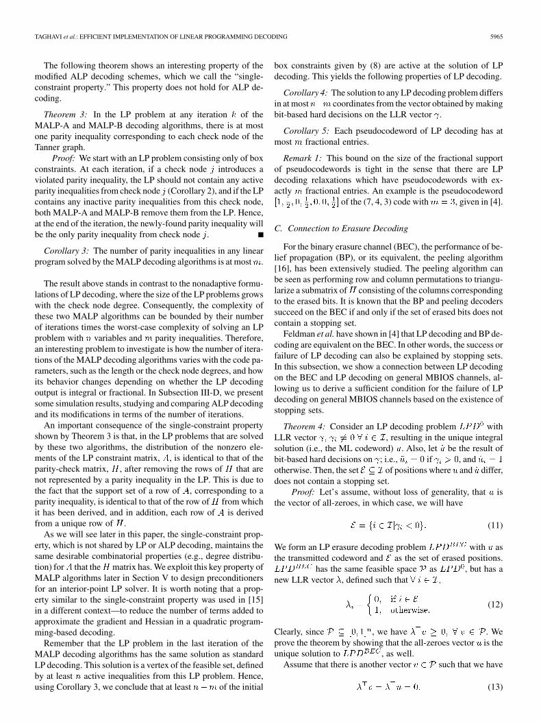
The following theorem shows an interesting property of themodified ALP decoding schemes, which we call the “single-constraint property.” This property does not hold for ALP de-coding.

Theorem 3: In the LP problem at any iteration of theMALP-A and MALP-B decoding algorithms, there is at mostone parity inequality corresponding to each check node of theTanner graph.

Proof: We start with an LP problem consisting only of boxconstraints. At each iteration, if a check node introduces aviolated parity inequality, the LP should not contain any activeparity inequalities from check node (Corollary 2), and if the LPcontains any inactive parity inequalities from this check node,both MALP-A and MALP-B remove them from the LP. Hence,at the end of the iteration, the newly-found parity inequality willbe the only parity inequality from check node .

Corollary 3: The number of parity inequalities in any linearprogram solved by the MALP decoding algorithms is at most .

The result above stands in contrast to the nonadaptive formu-lations of LP decoding, where the size of the LP problems growswith the check node degree. Consequently, the complexity ofthese two MALP algorithms can be bounded by their numberof iterations times the worst-case complexity of solving an LPproblem with variables and parity inequalities. Therefore,an interesting problem to investigate is how the number of itera-tions of the MALP decoding algorithms varies with the code pa-rameters, such as the length or the check node degrees, and howits behavior changes depending on whether the LP decodingoutput is integral or fractional. In Subsection III-D, we presentsome simulation results, studying and comparing ALP decodingand its modifications in terms of the number of iterations.

An important consequence of the single-constraint propertyshown by Theorem 3 is that, in the LP problems that are solvedby these two algorithms, the distribution of the nonzero ele-ments of the LP constraint matrix, , is identical to that of theparity-check matrix, , after removing the rows of that arenot represented by a parity inequality in the LP. This is due tothe fact that the support set of a row of , corresponding to aparity inequality, is identical to that of the row of from whichit has been derived, and in addition, each row of is derivedfrom a unique row of .

As we will see later in this paper, the single-constraint prop-erty, which is not shared by LP or ALP decoding, maintains thesame desirable combinatorial properties (e.g., degree distribu-tion) for that the matrix has. We exploit this key property ofMALP algorithms later in Section V to design preconditionersfor an interior-point LP solver. It is worth noting that a prop-erty similar to the single-constraint property was used in [15]in a different context—to reduce the number of terms added toapproximate the gradient and Hessian in a quadratic program-ming-based decoding.

Remember that the LP problem in the last iteration of theMALP decoding algorithms has the same solution as standardLP decoding. This solution is a vertex of the feasible set, definedby at least active inequalities from this LP problem. Hence,using Corollary 3, we conclude that at least of the initial

box constraints given by (8) are active at the solution of LPdecoding. This yields the following properties of LP decoding.

Corollary 4: The solution to any LP decoding problem differsin at most coordinates from the vector obtained by makingbit-based hard decisions on the LLR vector .

Corollary 5: Each pseudocodeword of LP decoding has atmost fractional entries.

Remark 1: This bound on the size of the fractional supportof pseudocodewords is tight in the sense that there are LPdecoding relaxations which have pseudocodewords with ex-actly fractional entries. An example is the pseudocodeword

of the (7, 4, 3) code with , given in [4].

C. Connection to Erasure Decoding

For the binary erasure channel (BEC), the performance of be-lief propagation (BP), or its equivalent, the peeling algorithm[16], has been extensively studied. The peeling algorithm canbe seen as performing row and column permutations to triangu-larize a submatrix of consisting of the columns correspondingto the erased bits. It is known that the BP and peeling decoderssucceed on the BEC if and only if the set of erased bits does notcontain a stopping set.

Feldman et al. have shown in [4] that LP decoding and BP de-coding are equivalent on the BEC. In other words, the success orfailure of LP decoding can also be explained by stopping sets.In this subsection, we show a connection between LP decodingon the BEC and LP decoding on general MBIOS channels, al-lowing us to derive a sufficient condition for the failure of LPdecoding on general MBIOS channels based on the existence ofstopping sets.

Theorem 4: Consider an LP decoding problem withLLR vector , resulting in the unique integralsolution (i.e., the ML codeword) . Also, let be the result ofbit-based hard decisions on ; i.e., if , andotherwise. Then, the set of positions where and differ,does not contain a stopping set.

Proof: Let’s assume, without loss of generality, that isthe vector of all-zeroes, in which case, we will have

(11)

We form an LP erasure decoding problem with asthe transmitted codeword and as the set of erased positions.

has the same feasible space as , but has anew LLR vector , defined such that

(12)

Clearly, since , we have . Weprove the theorem by showing that the all-zeroes vector is theunique solution to , as well.

Assume that there is another vector such that we have

(13)


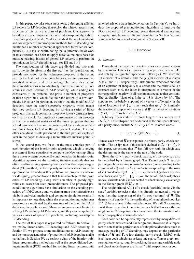
Fig. 1. Histograms of the number of iterations for ALP, MALP-A, and MALP-B decoding for a random (3,6)-regular LDPC code of length 480 at �� dB.The left, middle, and right columns respectively correspond to the results of all decoding instances, decodings with integral outputs, and decodings with fractionaloutput.

Combining (12) and (13) yields

(14)

implying that . Therefore, using (11), the costof the vector for will be

(15)

with equality if and only if . Since, by as-sumption, is the unique solution to , we must have

. Hence, is also the unique solution to. Finally, due to the equivalence of LP and BP decod-

ings on the BEC, we conclude that does not contain a stoppingset.

Theorem 4 will be used later in the paper to design an efficientway to solve the systems of linear equations we encounter in LPdecoding.

D. Simulation Results

We present simulation results for ALP, MALP-A, andMALP-B decoding of random (3,6)-regular LDPC codes,where the cycles of length four are removed from the Tannergraphs of the codes. The simulations are performed in anAWGN channel with the SNR of 2 dB (the threshold of be-lief-propagation decoding for the ensemble of (3,6)-regularcodes is 1.11 dB), and include 8 different lengths, with 1000trials at each length.

In Fig. 1, we have plotted the histograms of the number of it-erations using the three algorithms for length . The first

column of histograms includes the results of all the decodinginstances, while the second and third columns only include thedecoding instances with integral and fractional outputs, respec-tively. From this figure, we can see that when the output is in-tegral (second column), the three algorithms have a similar be-havior, and they all converge in less that 15 iterations. On theother hand, when the output is fractional (third column), thetypical numbers of iterations are 2–3 times higher for all algo-rithms, so that we observe two almost nonoverlapping peaks inthe histograms of the first column.

In Fig. 2, the average numbers of iterations of the three al-gorithms are plotted for both integral and fractional decodingoutputs versus the code length. We can observe that the numberof iterations for MALP-A and MALP-B decoding are signifi-cantly higher than that of ALP when the output is fractional.On the other hand, for decoding instances with integral outputs,where the LP decoder is successful in finding the ML codeword,the increase in the number of iterations for the modified ALPdecoders relative to the ALP decoder is very small. Hence, theMALP decoders pay a small price in terms of the number of iter-ations in exchange for obtaining the single-constraint property.

To measure the statistical deviation of the number of itera-tions from their mean, we computed the CDF of the numberof iterations for each scenario, and observed that for each of thedata points plotted in Fig. 2, the 95th percentile value is between2.5–6 iterations above the mean value. Moreover, our simula-tions indicate that in the scenario examined in Fig. 1, the size ofthe largest LP that is solved in each MALP-A or MALP-B de-coding problem is smaller on average than that of ALP decodingby 17% for integral outputs and 30% for fractional outputs.

The overall execution times of these decoding algorithmsheavily depend on the choice of the underlying LP solver.Using the simplex algorithm implementation in GLPK [19],we have observed that the overall execution times of the ALP


Fig. 2. Number of iterations of ALP, MALP-A, and MALP-B decoding versus code length for random (3,6)-regular LDPC codes at �� dB. The solidcurves represent the decoding instances with integral outputs, and the dashed curves represent the decoding instances with fractional outputs.

and MALP algorithms are very comparable, with MALP al-gorithms sometime performing slightly faster than ALP. For acomparison of the execution time of ALP and a number of otherLP decoding approaches, we refer the reader to the simulationresults in Section III of [10].

IV. SOLVING THE LP USING THE INTERIOR-POINT METHOD

General-purpose LP solvers do not take advantage of theparticular structure of the optimization problems arising in LPdecoding, and, therefore, using them can be highly inefficient.In this and the next sections, we investigate how LP algorithmscan be implemented efficiently for LP decoding. The two majortechniques for linear optimization used in most applicationsare Dantzig’s simplex algorithm [20] and the interior-pointmethods.

A. Simplex Versus Interior-Point Algorithms

The simplex algorithm takes advantage of the fact that thesolution to an LP is at one of the vertices of the feasible polyhe-dron. Starting from a vertex of the feasible polyhedron, it movesin each iteration (pivot) to an adjacent vertex, until an optimalvertex is reached. Each iteration involves selecting an adjacentvertex with a lower cost, and computing the size of the step totake in order to move to that edge, and these are computed by anumber of matrix and vector operations.

Interior-point methods generally move along a path within theinterior of the feasible region. Starting from an interior point,these methods approximate the feasible region in each iterationand take a Newton-type step towards the next point, until theyget to the optimum point. Computation of these steps involvessolving a linear system.

The complexity of an LP solver is determined by the numberof iterations it takes to converge and the average complexity ofeach iteration. The number of iterations of the simplex algorithmhas been observed to be polynomial (superlinear), on average,in the problem dimension , while its worst-case performancecan be exponential. An intuitive way of understanding why theaverage number of simplex pivots to successfully solve an LPdecoding problem is at least linear in is to note that each pivotmakes one basic primal variable nonbasic (i.e., sets it to zero)and makes one nonbasic variable basic (i.e., possibly increasesit from zero). Hence, starting from an initial point, it shouldgenerally take at least a constant times pivots to arrive at apoint corresponding to a binary codeword. Therefore, even ifthe computation of each simplex iteration were done in lineartime, one could not achieve a running time better that ,unless the simplex method is fundamentally revised.

In contrast to the simplex algorithm, for certain classes of in-terior-point methods, such as the path-following algorithm, theworst-case number of iterations has been shown to be ,although these algorithms typically converge in itera-tions [21]. Therefore, if the Newton step at each iteration can becomputed efficiently, taking advantage of the sparsity and struc-ture in the problem, one could obtain an algorithm that is fasterthan the simplex algorithm for large-scale problems.

Interior-point methods consist of a variety of algorithms, dif-fering in the way the optimization problem is approximated byan unconstrained problem, and how the step is calculated at eachiteration. One of the most successful classes of interior-pointmethods is the primal-dual path-following algorithm, which ismost effective for large-scale applications. In the following sub-section we present a brief review of this algorithm. For a more


comprehensive description, we refer the reader to the literatureon linear programming and interior-point methods, e.g., [21].

B. Primal-Dual Path-Following Algorithm

For simplicity, in this section we assume that the LP problemsthat we want to solve are of the form (9). However, by intro-ducing a number of additional slack variables, we can modifyall the expressions in a straighforward way to represent the casewhere both types of box constraints may be present for eachvariable.

We first write the LP problem with variables and con-straints in the “augmented” form

(16)

Here, to convert the LP problem (9) into the form above, wehave taken two steps. First, noting that each variable in (9)is subject to exactly one box constraint of the form or

, we introduce the variable vector and cost vector ,such that for any and if theformer inequality is included (i.e., ), andand , otherwise. Therefore, the box constraints willall have the form , and the coefficients of the parityinequalities will also change correspondingly. Second, for any

we convert the parity inequality in(9), where denotes the th row of , to a linear equation

by introducing nonnegative slack variables, where , with corresponding coefficients

equal to zero in the cost vector . We will sometimes refer to thefirst (nonslack) variables as the standard variables. The dualof the primal LP has the form

(17)

where and are the dual standard and slack variables,respectively.

The first step in solving the primal and dual problems is to re-move the inequality constraints by introducing logarithmic bar-rier terms into their objective functions.3 The primal and dualobjective functions will thus change to and

, respectively, for some , resulting ina family of convex nonlinear barrier problems , parameter-ized by , that approximate the original linear program4 Sincethe logarithmic term forces and to remain positive, the so-lution to the barrier problem is feasible for the primal-dual LP,and it can be shown that as , it approaches the solution tothe LP problem. The key idea of the path-following algorithmis to start with some , and reduce it at each iteration, aswe take one step to solve the barrier problem.

3Because of this step, interior-point methods are sometime referred to in theliterature as barrier methods.

4In all equations throughout the paper, we use natural logarithms.

The Karush–Kuhn–Tucker (KKT) conditions provide neces-sary and sufficient optimality conditions for , and can bewritten as [21, Chapter 9]

(18)

(19)

(20)

(21)

where and are diagonal matrices with the entries of andon their diagonal, respectively, and denotes the all-ones vector.If we define

where is the current primal-dual iterate, theproblem of solving reduces to finding the (unique) zeroof the multivariate function . In Newton’s method, isiteratively approximated by its first-order Taylor series expan-sion around

(22)

where is the Jacobian matrix of . The Newton di-rection is obtained by setting theright-hand side of (22) to zero, resulting in the following systemof linear equations:

(23)

where , andare the residuals of the KKT equations (18), and is

the value of at iteration . If we start from a primal and dualfeasible point, we will not need to compute and , as theywill remain zero throughout the algorithm. However, for sake ofgenerality, here we do not make any feasibility assumption, inorder to have the flexibility to apply the equations in the general,possibly infeasible case.

In the case where the LP in (16) represents an LP decodingproblem, the linear system (23) has vari-ables and equations, where and , as defined earlier, denotethe number of parity inequalities and the code length, respec-tively.

The solution to the linear system (23) is given by

(24)

(25)

(26)

where

(27)


To simplify the notation, we will henceforth drop the subscriptfrom , but it should be noted that is a function of the

iteration number, . Having the Newton direction, the solutionis updated as

(28)

(29)

(30)

and the primal and dual step lengths, , are chosensuch that all the entries of and remain nonnegative. In ourexperiments, we have selected these step sizes according to thefollowing equations [21]

(31)

(32)

where . Specifically, we have found that a value closeto 0.5 is often a good choice for .

Since we are interested in solving the LP and not the bar-rier program for a particular , rather than taking manyNewton steps to approach the solution to , we reduce thevalue of each time a Newton step is taken, so that the barrierprogram gives a better approximation of the LP. A reasonableupdating rule for is to make it proportional to the duality gap

(33)

that is, to update according to

(34)

The primal-dual path-following algorithm described abovewill iterate until the duality gap becomes sufficiently small; i.e.,

. It has been shown that with a proper choice of thestep lengths, this algorithm takes to reduce theduality gap from to .

In a feasible implementation of the algorithm, in order to ini-tialize the algorithm, we need some feasible , and

. Obtaining such an initial point is nontrivial, and is usu-ally done by introducing a few dummy variables, as well as afew rows and columns to the constraint matrix. This may notbe desirable for a sparse LP, since the new rows and columnswill not generally be sparse. Furthermore, if the Newton direc-tions are computed based on the feasibility assumption; i.e., that

and , round-off errors can cause instabilities dueto the gradual loss of feasibility. As an alternative, an infeasibleimplementation of the primal-dual path-following algorithm isoften used, where any , and can be usedfor initialization. This algorithm will simultaneously try to re-duce the duality gap and the primal-dual feasibility gap to zero.Consequently, the termination criterion will change: we stop thealgorithm if , and . As men-tioned earlier, the other difference between the formulation ofthe feasible and infeasible implementations is that in the formercase, the residual vectors and can be replaced by zero vec-tors in (23).

C. Computing the Newton Directions: PreconditionedConjugate Gradient Method

The most complex step at each iteration of the interior-pointalgorithm in the previous subsection is to solve the “normal”system of linear equations in (24). While these equations werederived for the primal-dual path-following algorithm, in mostother variations of interior-point methods, we encounter linearsystems of similar forms, as well.

Algorithms for solving linear systems fall into two main cat-egories of direct methods and iterative methods. While directmethods, such as Gaussian elimination, attempt to solve thesystem in a finite number of steps and are exact in the absence ofrounding errors, iterative methods start from an initial guess andderive a sequence of approximate solutions. Since the constraintmatrix in (24) is symmetric and positive definite, themost common direct method for solving this problem is basedon computing the Cholesky decomposition of this matrix. How-ever, this approach is inefficient for large-scale sparse problemsdue to the computational cost of the decomposition, as well asloss of sparsity. Hence, in many LP problems, e.g., network flowlinear programs, iterative methods such as the conjugate gra-dient (CG) method [22] are preferred.

Suppose we want to find the solution to a system of linearequations given by

(35)

where is a symmetric positive definite matrix. Equiva-lently, is the unique minimizer of the functional

(36)

We call two nonzero vectors, -conjugate if

(37)

The CG method is based on building a set of -conjugate basisvectors , and computing the solution as

(38)

where . Hence, the problem becomes that offinding a suitable set of basis vectors. In the CG method, thesevectors are found in an iterative way, such that at step , the nextbasis vector is chosen to be the closest vector to the negativegradient of at the current point , under the condition thatit is -conjugate to . For a more comprehensivedescription of this algorithm, the reader is referred to [23].

While in principle the CG algorithm requires steps to findthe exact solution , sometimes a much smaller number of it-erations provides a sufficiently accurate approximation to thesolution. The distribution of the eigenvalues of the coefficientmatrix has a crucial effect on the convergence behavior of the


Fig. 3. Parameters � � � , and � , for � � �� at four iterations of the interior-point method for an LP subproblem of MALP decoding with � � ��

� � �� . The variable indices, �, (horizontal axis) are permuted to sort � in increasing order.

CG method (as well as many other iterative algorithms). In par-ticular, it is shown that [23, Chapter 6]

(39)

where and is the spectral conditionnumber of Q, i.e., the ratio of the maximum and minimum eigen-values of Q. Using this result, the number of iterations of the CGmethod required to reduce by a certain factor from itsinitial value can be upper-bounded by a constant times .We henceforth call a matrix ill-conditioned, in loose terms, ifCG converges slowly in solving (35).

In the interior-point algorithm, the spectral behavior ofchanges as a function of the diagonal elements,

of , which are, as described in the previoussubsection, the square roots of the ratios between the primalvariables and the dual slack variables . In Fig. 3, theevolution of the distributions of , and throughthe iterations of the interior-point algorithm is illustrated foran LP subproblem of an MALP decoding instance. We canobserve in this figure that and are distributed in such a waythat the product is relatively constant over all .This means that, although the path-following algorithm doesnot completely solve the barrier problems defined in IV-B, thecondition (20) is approximately satisfied for all . A conse-quence of this, which can also be observed in Fig. 3, is that

(40)

As the iterates of the interior-point algorithm become closer tothe solution and approaches zero, many of the ’s take verysmall or very large values, depending on the value of the cor-responding in the solution. This has a negative effect on thespectral behavior of , and as a result, on the convergence ofthe CG method.

When the coefficient matrix of the system of linear equa-tions is ill-conditioned, it is common to use preconditioning. Inthis method, we use a symmetric positive-definite matrix asan approximation of , and instead of (35), we solve the equiv-alent preconditioned system

(41)

We hence obtain the preconditioned conjugate gradient (PCG)algorithm, summarized as Algorithm 4.

Algorithm 4 Preconditioned Conjugate Gradient (PCG)

1: Compute an initial guess for the solution;2: ;3: Solve ;4: ;5: for until convergence do6: ;7: ;8: ;9: ;

10: Solve ;11: ;12: ;13: end for


In order to obtain an efficient PCG algorithm, we need thepreconditioner to satisfy two requirements. First,should have a better spectral distribution than , so that thepreconditioned system can be solved faster than the originalsystem. Second, it should be inexpensive to solve ,since we need to solve a system of this form at each step of thepreconditioned algorithm. Therefore, a natural approach is todesign a preconditioner which, in addition to providing a goodapproximation of , has an underlying structure that makes itpossible to solve using a direct method in linear time.

The convergence of the PCG algorithm can be determinedbased on the relative residual error

(42)

To ensure sufficient accuracy in the calculation of the Newtonsteps, one can stop the PCG algorithm once this residual value isbelow a certain threshold. The proper value of the threshold de-pends on the properties of the LP problem (such as code lengthand SNR in LP decoding), as well as the distance of the currentinterior-point from the optimum; the closer we are to the op-timum, the higher the accuracy needed in the calculation of theNewton steps.

One important application of the PCG algorithm is in inte-rior-point implementations of LP for minimum-cost networkflow (MCNF) problems. For these problems, the constraint ma-trix in the primal LP corresponds to the node-arc adjacencymatrix of the network graph. In other words, the LP primal vari-ables represent the edges, each constraint is defined for the edgesincident to a node, and the diagonal elements, of thediagonal matrix can be interpreted as weights for the edges(variables). A common method for designing a preconditionerfor is to select a set of columns of (edges) withlarge weights, and form , where the subscript

for a matrix denotes a matrix consisting of the columns ofthe original matrix with indices in .

It is known that at a nondegenerate solution to an MCNFproblem, the nonzero variables (i.e., the basic variables) corre-spond to a spanning tree in the graph. This means that, when theinterior-point method approaches such a solution, the weights ofall the edges, except those defining this spanning tree, will go tozero. Hence, a natural selection for would be the set of in-dices of the spanning tree with the maximum total weight, whichresults in the maximum-weight spanning tree (MST) precondi-tioner. Finding the maximum-weight spanning tree in a graphcan be done efficiently in linear time, and besides, due to the treestructure of the graph represented by , the matrix can beinverted in linear time, as well.5 The MST has been observed inpractice to be very effective, especially at the later iterations ofthe interior-point method, when the operating point is close tothe final solution.

V. PRECONDITIONER DESIGN FOR LP DECODING

Our framework for designing an effective preconditioner forLP decoding, similar to the MST preconditioner for MCNF

5Throughout the paper, we refer to solving a system of linear equations withcoefficient matrix � , in loose terms, as inverting � , although we do not ex-plicitly compute � .

Fig. 4. Extended Tanner graph for an LP problem with � � �� , and� � �.

problems, is to find a preconditioning set, ,corresponding to columns of and , resulting inmatrices and , such that is botheasily invertible and a good approximation of . Tosatisfy these requirements, it is natural to select to includethe variables with the highest weights, , while keeping

and full rank and invertible in time. Then, thesolution to in the PCG algorithm can befound by sequentially solving ,and , for , and , respectively.

We are interested in having a graph representation for theconstraints and variables of a linear program of the form (16) inthe LP decoding problem, such that the selection of a desirable

can be interpreted as searching for a subgraph with certaincombinatorial structures.

Definition 2: Consider an LP of the form (16) with con-straints and variables, where are slack variables.The extended Tanner graph of this LP is a bipartite graph con-sisting of variable nodes and constraint nodes, such thatvariable node is connected to constraint node iff is in-volved in the th constraint; i.e., is nonzero.

For the linear programs in the MALP decoding algorithms,since each constraint is derived from a unique check node ofthe original Tanner graph, the extended Tanner graph will be asubgraph of the Tanner graph, with the addition of degree-1(slack) variable nodes, each connected to one of the constraintnodes. In general, for an iteration of MALP decoding of a codewith an parity-check matrix, the extended Tanner graphswould contain constraint nodes, variable nodes cor-responding to the standard variables (bit positions), and slackvariable nodes. As extended Tanner graphs are special cases ofTanner graphs, they inherit all the combinatorial concepts de-fined for Tanner graphs, such as stopping sets. A small exampleof an extended Tanner graph is given in Fig. 4.

A. Preconditioning via Triangulation

For a sparse constraint matrix, , a sufficient condition forand to be invertible in time is that can

be made upper or lower triangular, with nonzero diagonal el-ements, using column and/or row permutations. We call a pre-conditioning set that satisfies this property a triangular set.Once an upper- (lower-) triangular form of is found,we start from the last (first) row of , and, by taking advan-tage of the sparsity, solve for the variable corresponding to the


diagonal element of each row recursively in time. It is notdifficult to see that there always exists at least one triangular setfor any LP decoding problem; one example is the set of columnscorresponding to the slack variables, which results in a diagonal

.As a criterion for finding the best approximation

of , we search for the triangular setthat contains the columns with the highest weights, . Onecan consider different strategies of scoring a triangular setfrom the weights of its members, e.g., the sum of the weights,or the largest value of minimum weight. It is interesting tostudy as a future work whether given any such metric, the“maximum-weight” (or optimal) triangular set can be found inpolynomial time. However, in this work, we propose a (subop-timal) greedy approach, which is motivated by the properties ofthe LP decoding problem.

The problem of bringing a parity-check matrix into (approx-imate) triangular form has been studied by Richardson and Ur-banke [24] in the context of the encoding of LDPC codes. Theauthors proposed a series of greedy algorithms that are sim-ilar to the peeling algorithm for decoding in the binary erasurechannel: repeatedly select a nonzero entry (edge) of the matrix(graph) lying on a weight-1 (degree-1) column or row (variableor check node), and remove both the column and row of thisentry from the matrix. They showed that parity-check matricesthat are optimized for erasure decoding can be made almost tri-angular using this greedy approach. It is important to note thatthis combinatorial approach only relies on the placement of thenonzero entries of the matrix, rather than their values.

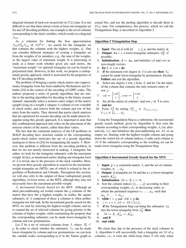
The fact that the constraint matrices of the LP problems inMALP decoding have structure similar to the correspondingparity-check matrix motivates the use of a greedy algorithmanalogous to those in [24] for triangulating the matrix . How-ever, this problem is different from the encoding problem, inthat we are not merely interested in making triangular, butrather, we look for the triangular submatrix with the maximumweight. In fact, as mentioned earlier, finding one triangular formof is trivial, due to the presence of the slack variables. Here,we present three greedy algorithms to search for the maximum-weight triangular set (MTS), one of which is related to the al-gorithms of Richardson and Urbanke. Throughout this section,we will also refer to the outputs of these (suboptimal) greedyalgorithms, in loose terms, as the MTS, although they may notnecessarily have the maximum possible weight.

1) Incremental Greedy Search for the MTS: Although anideal preconditioning set would contain the columns of thematrix that have the highest weights, in reality, the squaresubmatrix of composed of these columns is often neithertriangular nor full rank. In the incremental greedy search for theMTS, we start by selecting the highest-weight column, and tryto expand the set of selected columns by giving priority to thecolumns of higher weights, while maintaining the property thatthe corresponding submatrix can be made lower-triangular bycolumn and row permutations.

Let be a set of selected columns from , where. In order to check whether the submatrix can be made

lower-triangular by column and row permutations, we can treatthe variable nodes corresponding to in the Tanner graph as

erased bits, and use the peeling algorithm to decode them intime. For completeness, this process, which we call the

Triangulation Step, is described in Algorithm 5.

Algorithm 5 Triangulation Step

1: Input: The set with , and the matrix ;2: Output: An lower-triangular submatrix , if

possible;3: Initialization: , and initialize and as

zero-length vectors;4: for to do5: if the minimum row degree in is not one then

cannot be made lower-triangular by permutation; DeclareFailure and exit the algorithm;

6: Select any degree-1 row from , and let be the indexof the column that contains the only nonzero entry ofrow ;

7: ;

8: Set all the entries in column and row of to zero;9: end for

10: Form by setting;

Using the Triangulation Step as a subroutine, the incrementalgreedy search method, given by Algorithm 6, first sorts thecolumns according to their corresponding weights, (or, alter-natively, ), and initializes the preconditioning set, , as anempty set. Starting with the highest-weight column and goingdown the sorted list of column indices, it adds each column to

if the submatrix corresponding to the resulting set can bemade lower triangular using the Triangulation Step.

Algorithm 6 Incremental Greedy Search for the MTS

1: Input: constraint matrix , and the set of columnweights, ;

2: Output: A triangular set and the lower-triangularmatrix ;

3: Initialization: ;4: Sort the column indices according to their

corresponding weights, , in decreasing order, toobtain the permuted sequence , such that

;5: while and do6: ;7: if the Triangulation Step can bring the submatrix

into the lower-triangular form then8: ;9: end if

10: end while

We claim that, due to the presence of the slack columns in, Algorithm 6 will successfully find a triangular set of

columns; i.e., it exits the while-loop (lines 5–10) only when


. Assume, on the contrary, that the algorithm endswhile , so that the matrix is a lower-tri-angular matrix. This means that if we add any column

to , it cannot be made lower triangular, sinceotherwise, column would have already been added towhen in the while-loop.6 However, this clearly cannot bethe case, since we can produce a lower-triangular matrix

, simply by adding the columns corresponding to the slackvariables of the last rows of . Hence, we concludethat .

2) Column-Wise Greedy Search for the MTS: Algorithm 7is a column-wise greedy search for the MTS. It successivelyadds the index of the maximum-weight degree-1 column of tothe set , and eliminates this column and the row that sharesits only nonzero entry. Matrix initially contains degree-1slack columns, and at each iteration, one such column will beerased. Hence, there is always a degree-1 column in the residualmatrix, and the algorithm proceeds until columns are selected.The resulting preconditioning set will correspond to an upper-triangular submatrix .

Algorithm 7 Column-wise Greedy Search for the MTS

1: Input: constraint matrix , and the set of columnweights ;

2: Output: A triangular set and the upper-triangularmatrix ;

3: Initialization: , and initialize andas zero-length vectors;

4: Define and form as the index set of all degree-1columns in ;

5: for to do6: Let be the index of the (degree-1) column of

with the maximum weight, , and let be the index of therow that contains the only nonzero entry of this column;

7: ;

8: Set all the entries in row of (including the onlynonzero entry of column ) to zero;

9: Update from the residual matrix, ;10: end for11: Form by setting

;

3) Row-Wise Greedy Search for the MTS: Algorithm 7 usesa row-wise approach for finding the MTS. In this method, welook at the set of degree-1 rows, add to the indices of all thecolumns that intersect with these rows at nonzero entries, andeliminate these rows and columns from . Unlike the column-wise method, it is possible that, at some iteration, there is nodegree-1 row in the matrix. In this case, we repeatedly eliminatethe lowest-weight column, until there is at least one degree-1row.

6Note that if any set � of columns can be made lower triangular, any subsetof these columns can be made lower triangular, as well.

Algorithm 8 Row-wise Greedy Search for the MTS

1: Input: constraint matrix , and the set of columnweights ;

2: Output: A triangular set and the lower-triangularmatrix ;

3: Initialization: , and initialize andas zero-length vectors;

4: Define and form as the index set of all degree-1rows in ;

5: while is not all zeroes do6: if then7: Let be any degree-1 row of , and be the

index of the column that contains the only nonzero entryof this row;

8: ;

9: Set all the entries in column of (including the onlynonzero entry of row ) to zero, and update ;

10: else11: Let be the index of the nonzero column of with the

minimum weight, . Set all the entries in column tozero, and update ;

12: end if13: end while14: Diagonal Expansion: For each row of that is

not represented in , append to , and append, i.e., the index of the corresponding slack

column, to both and ;15: Form by setting

;

In addition to this difference, the number of columns in bythe end of this procedure is often slightly smaller that . Hence,we perform a “diagonal expansion” step at the end, where

columns corresponding to the slack variables are addedto , while keeping it a triangular set. A problem with thisexpansion method is that, since the algorithm does not have achoice in selecting the slack variables added in this step, it mayadd columns that have very small weights.

Let be the triangular submatrix obtained before the ex-pansion step. As an alternative to diagonally expanding byadding slack columns, we can apply a “triangular expansion.”In this method, we form a matrix consisting of the columns of

that do not share any nonzero entries with the rows in vector, and apply a column-wise or row-wise greedy search to this

matrix in order to obtain a high-weight lower-triangular sub-matrix . This requirement for forming ensures that theresulting triangular submatrices and can be concate-nated as

(43)

to form a larger triangular submatrix of . This process can becontinued, if necessary, until a square triangular matrix


is obtained, although our experiments indicate that one ex-pansion step is often sufficient to provide such a result. It is easyto see that this approach is potentially stronger than the diagonalexpansion in Algorithm 8, since it has the diagonal expansion asa special case.

B. Implementation and Complexity Considerations

To compute the running time of Algorithm 6, note that whileStep 4 has complexity, the computational complexityof the algorithm is dominated by the Triangulation Step. Thissubroutine has complexity, and is called times inAlgorithm 6, which makes the overall complexity . Aninteresting problem to investigate is whether we can simplifythe triangulation process in line 7 to have sublinear complexityby exploiting the results of the previous round of triangula-tion, as stated in the following open problem concerning erasuredecoding.

Open Problem: Consider the Tanner graph corresponding toan arbitrary LDPC code of length . Assume that a set of bitsare erased, and does not contain a stopping set in the Tannergraph. Thus, the decoder successfully recovers these erased bitsusing the peeling algorithm (i.e., the triangulation Algorithm 5).Now, we add a bit to the set of erased bits. Given , and thecomplete knowledge of the process of decoding , such as theorder in which the bits are decoded, and the check nodes used,is there an scheme to verify if can be decoded bythe peeling algorithm?

In addition to this potential simplification, it is possible tomake a number of modifications to Algorithm 6 in order to re-duce its complexity. Let be the size of the smallest stopping setin the extended Tanner graph of , which means that the subma-trix formed by any columns can be made triangular. Then,instead of initializing to be the empty set, we can immedi-ately add the highest-weight columns to , since we areguaranteed that can be made triangular. Moreover, at eachiteration of the algorithm, we can consider columns to beadded to , in order to reduce the number of calls to the trian-gulation subroutine. The value of can be adaptively selectedto make sure that the modified algorithm remains equivalent toAlgorithm 6.

To assess the complexity of Algorithm 7, we need to examineSteps 8 and 11 that involve column or row operations, as wellas Steps 4, 6, and 9 that deal with the list of degree-1 columns.Since there is an number of nonzero entries in each columnor row of , running Step 8 times (due to the for-loop) andderiving from in Step 11 each takes time. However,one should be careful in selecting a suitable data structure forstoring the set , since, in each cycle of the for-loop, weneed to extract the element with the maximum weight, and addto and remove from this set an number of elements. Byusing a binary heap data structure [25], which is implementableas an array, all these (Steps 6 and 9) can be done intime in the worst case. Also, the initial formation of the heap(Step 4) has complexity. As a result, the total complexityof Algorithm 7 becomes .

Similarly, in Algorithm 8, we need a mechanism to extractthe minimum-weight member of the set of remaining columns.

While the heap structure mentioned above works well here,since no column is added to the set of remaining columns, wecan alternatively sort the set of all columns by their weights asa preprocessing step with complexity, thus makingthe complexity of the while-loop linear. Since the complexityof Steps 15 (diagonal expansion) and 16 are linear, as well, thetotal running time of Algorithm 8 will be .

The process of finding a triangular preconditioner is per-formed at each iteration of the interior-point algorithm. Sincethe values of primal variables, , do not substantially changein one iteration, we expect the MTS at each iteration to be rel-atively close to that in the previous iteration. Consequently, aninteresting area for future work is to investigate modificationsof the proposed algorithms, where the knowledge of the MTS inthe previous iteration of the interior-point method is exploitedto improve the complexity of these algorithms.

VI. ANALYSIS OF THE MTS PRECONDITIONING ALGORITHMS

A. Performance Analysis

It is of great interest to study how the proposed algorithmsperform as the problem size goes to infinity. We expect that anumber of asymptotic results similar to those of Richardson andUrbanke in [24] can be derived, e.g., showing that the greedypreconditioner designs perform well for capacity-approachingLDPC ensembles. However, since one of the main advantagesof LP decoding over message-passing decoding is its geomet-rical structure that facilitates the analysis of its performance inthe finite-length regime, in this work we focus on studying theproposed algorithms in this regime.

We will study the behavior of the proposed preconditionerin the later iterations of the interior-point algorithm, when theiterates are close to the optimum. This is justified by the factthat, as the interior-point algorithm approaches the boundary ofthe feasible region during its later iterations, many of the primalvariables, , and the dual slack variables, , approach zero,thus deteriorating the conditioning of the matrix .This is when a precoditioner is most needed. In addition, we canobtain some information about the performance of the precon-ditioner in the later iterations by focusing on the optimal pointof the feasible set.

Consider an LP problem in the augmented form (16) as partof ALP or MALP decoding, and assume that it has a unique op-timal solution (although parts of our analysis can be extendedto the case with nonunique solutions). We denote by the triplet

the primal-dual solution to this LP, and byan intermediate iterate of the interior-point method. We can par-tition the set of the columns of into the basic set

(44)

and the nonbasic set

(45)

For brevity, we henceforth refer to the columns of the con-straint matrix corresponding to the basic variables as the“basic columns.” It is not difficult to show that, for an LPwith a unique solution, the number of basic variables, i.e.,

, is at most . To see this, assume that of the standard


variables are nonzero, which means that boxconstraints of the form are active at . Since isa vertex defined by at least active constraints in the LP, weconclude that at least parity inequalities must be active at ,thus leaving at most nonzero slack variables. We call theLP nondegenerate if , and degenerate if .

It is known that the unique solution is “strictlycomplementary” [26], meaning that for any ei-ther and , or and . Rememberingfrom (27) that , as the iterates of the interior-pointalgorithm approach the optimum, i.e., given in (34) goes tozero, we will have

(46)

Therefore, towards the end of the algorithm, the matrixwill be dominated by the columns of and cor-

responding to the basic set. Hence, it is highly desirable to se-lect a preconditioning set that includes all the basic columns,i.e., , in which case becomes a better andbetter approximation of as we approach the optimum of theLP. In the rest of this subsection, we will show that, when thesolution to the LP is integral and is sufficiently small, thisproperty can be achieved by low complexity algorithms similarto Algorithms 7 and 8.

Lemma 2: Consider the extended Tanner graph for an LPsubproblem of MALP decoding. If the primal solution to

is integral, the set of variable nodes corresponding to thebasic set, whose definition is based on the augmented form (16)of the LP, does not contain any stopping set.

Proof: Consider an erasure decoding problem on, where the basic variable nodes are erasures. We prove the

lemma by showing that the peeling (or LP) decoder can success-fully correct these erasures.

We denote by and the solutions to the primal LP in the(original) standard form (9) and in the augmented form (16).From part c) of Theorem 2, we know that is also the solutionto a full LP decoding problem with the LLR vectorand the Tanner graph comprising the standard variable nodesand the active check nodes, .

We partition the basic set into and , the sets ofbasic standard variables and basic slack variables, respectively.We also partition the set of check nodes in into and

, the sets of check nodes that generate the active and inac-tive parity inequalities of , respectively. Clearly, the neigh-bors of the slack variable nodes in are the check nodes in

, since an inactive parity inequality has, by definition, anonzero slack.

Step 1: We first show that, even if we remove the check nodesin from , the set of basic standard variable nodes, ,does not contain a stopping set.

Remembering the conversion of the LP in the standard form(9) with inequality constraints to the augmented form (16), wecan write

(47)

Using, as in Theorem 4, the notation for the result of bit-basedhard decision on , one can see that is identical to , the

set of positions where and differ. Hence, knowing thatis the solution to an LP decoding problem, and using Theorem4, we conclude that the set does not contain a stopping setin the Tanner graph that only includes the check nodes in .

Step 2: Now we return to , and consider solving ,where all the basic variables are erasures, using the peeling al-gorithm. Since the slack variables which are basic are connectedonly to the inactive check nodes, we know from Step 1 that theerased variables can be decoded by only using the activecheck nodes . Once these variable nodes are peeled off thegraph, we are left with the basic slack variable nodes, each ofwhich is connected to a distinct check node in . There-fore, the peeling algorithm can proceed by decoding all of thesevariables. This completes the proof.

Lemma 2 shows that, under proper conditions, the submatrixof formed by only including the columns corresponding

to the basic variables can be made lower triangular by columnand row permutations. This suggests that looking for a max-imum-weight triangular set is a natural approach for designinga preconditioner in MALP decoding. In particular, the followingtheorem shows that, under the conditions of Lemma 2, the in-cremental greedy Algorithm 6 indeed finds a preconditioningset that includes all such columns.

As the interior-point algorithm progresses, the basic variablesapproach 1, while the nonbasic variables approach zero. Hence,referring to (46), we see that after a large enough number ofiterations, the highest-weight columns of will correspondto the basic set . The following theorem shows that two ofthe proposed algorithms indeed find a preconditioning set thatincludes all such columns.

Theorem 5: Consider an LP subproblem of an MALPdecoding problem. If the primal solution to is integral,at the iterates of the interior-point method that are sufficientlyclose to the solution, both the Incremental Greedy Algorithmand the Row-wise Greedy Algorithm can successfully find atriangular set that includes all the columns corresponding to thebasic set.

Proof: As the interior-point algorithm progresses, theweights corresponding to the basic variables approach ,while the weights of nonbasic variables approach zero. Hence,when becomes sufficiently small, the columns correspondingto the basic set, will be the highest-weight columns of ,and according to Lemma 2, the matrix consisting of thesecolumns can be made triangular, provided that the solution to

is integral.In view of this result, the proof of the claim for the incre-

mental greedy algorithm becomes straighforward: The precon-ditioning set continues to grow by one member at each it-eration, at least until it includes all the highest-weight (i.e.,basic) columns.

To prove that the triangular set given by the row-wisegreedy algorithm includes the basic set, as well, it is sufficientto show that none of the basic columns will be erased from(i.e., become all zeroes) in line 11 of Algorithm 8. Assume that,at some iteration, a column is selected in line 11 to be erased.Column has the minimum weight among the nonzero columnscurrently in . Therefore, if is a basic column and is small


Fig. 5. Progress of the residual error for different PCG implementations, solving (24) in the �th iteration of the interior-point algorithm, in an LP with an integralsolution. The constraint matrix � has 713 rows and 2713 columns, � � ��, and �� .

enough, all the other nonzero columns are basic columns,as well, since the basic columns are the highest-weightcolumns of . This means that could be made triangular,without running out of degree-1 rows and having to erasecolumn . So, column cannot be basic.

Remark 2: The proof above suggests that Theorem 5 can bestated in more general terms. For any , let bea set consisting of the highest-weight columns of . Then, ifthe set of variable nodes corresponding to in the (extended)Tanner graph does not contain a stopping set, that is, canbe made triangular by row and column permutations, then thepreconditioning sets found by Algorithms 6 and 8 both contain

.The assumption that the solution is integral does not hold for

all LPs that we solve in adaptive LP decoding. On the otherhand, in practice, we are often interested in solving the LP ex-actly only when LP decoding finds an integral solution (i.e.,the ML codeword). This, of course, does not mean that in suchcases every LP subproblem solved in the adaptive method hasan integral solution. However, one can argue heuristically that,if the final LP subproblem has an integral solution, the interme-diate LPs are also very likely to have an integral solution. Tosee this, remember from Theorem 2 that each intermediate LPproblem that is solved in adaptive LP decoding is equivalent toa full LP decoding that uses a subset of the check nodes in theTanner graph. Now, if LP decoding with the complete Tannergraph has an integral solution, it is natural to expect that, afterremoving a subset of check nodes, which can also reduce thenumber of cycles, the LP decoder is still very likely to find anintegral solution.

B. Performance Simulation

We simulated the LP decoding of (3,6)-regular LDPCcodes on the AWGN channel using the MALP-A algorithm

and our sparse implementation of the path-following inte-rior-point method. We have shown earlier that, as interior-pointprogresses, the matrix that needs to be inverted to com-pute the Newton steps becomes more and more ill-conditioned.We have observed that this problem becomes more severe inthe later iterations of the MALP-A algorithm, where the LPproblem is larger and more degenerate due to the abundance ofactive constraints at the optimum solution of the problem.

In Figs. 5–8, we present the performance results of the PCGmethod for four different systems of linear equations in theform of (24), solved in the infeasible primal-dual path-fol-lowing interior-point algorithm, using the preconditionersdesigned by greedy Algorithms 6–8.7 In these simulations,we used a randomly-generated (3,6)-regular LDPC code oflength 2000, where the cycles of length four were removed. Wehave measured the performance of the PCG algorithm by thebehavior of the relative residual error , defined in (42)as a function of the iteration number of the PCG algorithm.In our experiments, we often start with a threshold on thiserror in the range 0.05–0.1, and in the latter iterations of theinterior-point method, we reduce this threshold to a level in therange 0.001–0.01.

In Figs. 5 and 6, we considered solving (24) in two differentiterations of the interior-point algorithm for solving an LPproblem. This LP problem was selected at the 6th iterationof an MALP decoding problem at dB, and thesolution to the LP was integral. The constraint matrix forthis LP had 713 rows and 2713 columns, and we used the PCGalgorithm to compute the Newton step. Fig. 5 corresponds tofinding the Newton step at the 8th iteration of the interior-pointalgorithm. In this scenario, the duality gap was

7In all the simulations of the Row-wise Greedy Search (Algorithm 8) thatwe present in this section, we have used a diagonal expansion, rather than atriangular expansion, as described in Subsection V-A.


Fig. 6. Progress of the residual error for different PCG implementations, solving (24) in the 18th iteration of the interior-point algorithm, in an LP with an integralsolution. The constraint matrix � has 713 rows and 2713 columns, � � ��, and �� .

Fig. 7. Progress of the residual error for different PCG implementations, solving (24) in the 8th iteration of the interior-point algorithm, in an LP with a fractionalsolution. The constraint matrix � has 830 rows and 3830 columns, � � ��, and �� .

equal to 48.6, and the condition number of the problemwas equal to . We have plotted the residual errorof the CG method without preconditioning, as well as thePCG method using the three proposed preconditioner designs.For this problem, except during the first 10-15 iterations, thebehaviors of the three preconditioned implementations are verysimilar, and all significantly outperform the CG method.

In Fig. 6, we solved (24) at the th iteration of the same LP,where the interior-point is much closer to the solution, with

and . In this problem, the convergenceof the CG method is very slow, so that in 200 iterations, theresidual error does not get below 0.07. The PCG method with

incremental greedy preconditioning, reaching a residual error ofin 40 iterations, has the fastest convergence, followed by

the column-wise greedy preconditioner.To study the performance of the algorithms when the LP solu-

tion is not integral, we considered an LP from the 6th iterationof an MALP-A decoding problem at dB, wherethe solution was fractional. The matrix had 830 rows and3830 columns. Fig. 7 corresponds to the th iteration of the in-terior-point algorithm, with and ,while Fig. 8 corresponds to the 18th (penultimate) iteration, with

and . These parameters arechosen such that the scenarios in these two figures are respec-


Fig. 8. Progress of the residual error for different PCG implementations, solving (24) in the 18th iteration of the interior-point algorithm, in an LP with a fractionalsolution. The constraint matrix � has 830 rows and 3830 columns, � � ��, and �� .

tively similar to those in Figs. 5 and 6, the main difference beingthat the decoding problem now has a fractional solution. We canobserve that, while the performance of the CG method is verysimilar in Figs. 5 and 7, as well as in Figs. 6 and 8, the precon-ditioned implementations have slower convergence when theLP solution is fractional. In particular, in Fig. 8, the row-wisegreedy preconditioner does not improve the convergence of theCG method, and is essentially ineffective.

To provide an overall perspective on the behavior of LP de-coding using the schemes proposed here, in Fig. 9 we haveplotted three different parameters as a function of the iterationindex of the interior-point method as it steps toward the solu-tion. The numbers are obtained from a single instance of LPdecoding of a (3,6)-regular LDPC code of length 1920 at SNR= 2 dB, as a representative of the typical behavior of a suc-cessful decoding scenario at a moderate SNR. The decoding wasdone using the MALP-A decoding method and the column-wisegreedy preconditioning algorithm. In this decoding instance,MALP-A took 5 iterations (i.e., solved 5 LP subproblems) tofind the correct codeword, and we have plotted the results forthe first, third, and fifth (final) iterations. The plots show thenumber of PCG iterations it took to compute the Newton step,the objective function gap (the objective function defined in (9)and (16) with its optimum value subtracted) and the currentvalue of the duality gap (as defined in (33)). We observe thatwhile the objective function and duality gaps decrease exponen-tially as the interior-point method progresses, the convergenceof the PCG method becomes faster, although the system of linearequations to obtain the Newton steps becomes more and moreill-conditioned.

C. Discussion

Overall, we have observed that in very ill-conditioned prob-lems, the incremental and the column-wise greedy algorithms

are significantly more effective than the row-wise greedy al-gorithm in speeding up the solution of the linear system. Thebetter performance of the column-wise approach relative to therow-wise approach can be explained by the fact that the former,which searches for degree-1 columns, has more choices at eachstage, since the columns of have lower degrees on averagethan its rows. Besides, while the column-wise algorithm is al-ways able to find a complete triangular preconditioning set, therow-wise algorithm needs to expand the preconditioning set atthe end by adding some slack columns that may have very lowweights. Considering both the complexity and performance, thecolumn-wise search (Algorithm 7) seems to be a suitable choicefor a practical implementation of LP decoding.

A second observation that we have made in our simulationsis that the convergence of the PCG method cannot be well char-acterized just by the condition number of the preconditionedmatrix. In fact, we have encountered several situations wherethe preconditioned matrix had a much higher condition numberthan the original matrix, yet it resulted in a much faster conver-gence. For instance, in the scenario studied in Fig. 8, the condi-tion number of the preconditioned matrix for both thecolumn-wise and the incremental algorithms was higher thanthat of by a factor of 50–100, while these preconditioners stillimproved the convergence compared to the CG method. Indeed,the literature suggests that the speed of convergence of the CGcan typically be better explained by the number of distinct clus-ters of eigenvalues.

While we studied the interior-point method in the context ofMALP decoding, the proposed algorithms can also be appliedto the LPs that may have more than one constraint from eachcheck node. For instance, we have observed that the proposedimplementation is also very effective for ALP decoding. How-ever, in the absence of the single-constraint property, some ofthe analytical results we presented may no longer be valid.


VII. SUMMARY OF THE PROPOSED LP DECODING ALGORITHM

In this paper, we have proposed and studied a number of al-gorithms that can be used either jointly or separately in dif-ferent stages of LP decoding, as well as in other applicationsinvolving optimization or systems of linear equations. To pro-vide a high-level overview of an end-to-end LP decoder basedon these algorithms, we present in Algorithm 9 a sketch of an LPdecoder employing the following techniques: adaptive LP de-coding (ALP/MALP), an interior-point method for solving LPs,a preconditioned conjugate-gradient method (PCG) to computeNewton steps, and a greedy preconditioner design algorithm.

Algorithm 9 The sketch of an end-to-end LP decoder

1: Setup the initial LP problem with box constraints from(8);

2: repeat ALP/MALP Loop; based, e.g., on Algorithm 33: Obtain the the augmented primal (16) and dual (17)

forms of the current LP problem;4: Find initial values , and for the primal

and dual standard and slack variables, and an initial valuefor the barrier coefficient (Lagrange multiplier);

5: repeat Interior-point method loop to solve the currentLP; e.g., based on the primal-dual path-followingalgorithm described in Subsection IV-B

6: Form the normal equation (24) to compute the Newtonstep for the dual standard variables, ;

7: Find a triangular set —defined inSubsection V-A—using one of the greedy searchAlgorithms 6, 7, or 8;

8: Using , obtain the preconditioner matrix;

9: Perform the PCG method—based on Algorithm 4—tosolve for in (24), using the preconditioner ;

10: Given , obtain the remaining two Newton stepsand using (25) and (26);

11: Calculate the primal and dual step sizes andusing (31)–(32), and update , and using (28)–(30);

12: Update the barrier coefficient (Lagrange multiplier)according to (34);

13: Compute the duality gap as defined in (33), andfeasibility gap with anddefined in (23);

14: until Duality gap and feasibility gap are below theircorresponding thresholds

15: Given the solution to the current LP, search the set oflinear constraints of LP decoding (7)—using Algorithm2—to find all cuts (violated constraints) at this solution;

16: If any cuts were found, add them to the LP problem,and remove all or some of the inactive constraints fromthe LP problem, according to MALP-A (Algorithm 3)or MALP-B;

17: until No cuts are found18: Output the solution of the final LP as the LP decoding

solution.

VIII. CONCLUSIONS

In this paper, we studied various elements in an efficientimplementation of LP decoding. We first studied the adaptiveLP decoding algorithm and two variations and demonstrateda number of properties of these algorithms. Specifically, weproposed modifications of the ALP decoding algorithm thatsatisfy the single-constraint property; i.e., each LP to be solvedcontains at most one parity inequality from each check node ofthe Tanner graph.

We then studied a sparse interior-point implementation oflinear programming, with the goal of exploiting the propertiesof the decoding problem in order to achieve lower complexity.The heart of the interior-point algorithm is the computation ofthe Newton step via solving an (often ill-conditioned) system oflinear equations. Since iterative algorithms for solving sparselinear systems, including the conjugate-gradient method, con-verge slowly when the system is ill-conditioned, we focused onfinding a suitable preconditioner to speed up the process.

Motivated by the properties of LP decoding, we studied anew framework for desiging a preconditioner. Our approach wasbased on finding a square submatrix of the LP constraint matrixwhich contains the columns with the highest possible weights,and at the same time, can be made lower- or upper-triangularby column and row permutations, making it invertible in lineartime. We proposed a number of greedy algorithms for designingsuch preconditioners, and proved that, when the solution to theLP is integral, two of these algorithms indeed result in effec-tive preconditioners. We demonstrated the performance of theproposed schemes via simulation, and we observed that the pre-conditioned systems are most effective when the current LP hasan integral solution.

One can imagine various modifications and alternatives to theproposed greedy algorithms for designing preconditioners. It isalso interesting to investigate the possibility of finding otheradaptive or nonadaptive formulations of LP decoding that re-sult in solving the smallest possible number of LPs, while main-taining the single-constraint property. Moreover, there are sev-eral aspects of the implementation of LP decoding that are notexplored in this work. These potential areas for future researchinclude the optimal selection of the stopping criteria and stepsizes for the interior-point algorithm and the CG method, aswell as the theoretical analysis of the effect of preconditioningon the condition number and the eigenvalue spectrum of thelinear system, similar to the study done in [27] for network flowproblems.

APPENDIX APROOF OF THEOREM 2

a) To prove the claim, we show that the solution to any linearprogram consisting of the initial (single-sided) boxinequalities given by (8) and any number of parity in-equalities of the form (6) satisfies all the double-sided boxconstraints of the form .For simplicity, we first transform each variable ,


Fig. 9. Behavior of the interior-point method using PCG with column-wise greedy preconditioner search. The results are plotted for solving 3 LP subproblems atdifferent iterations of the same MALP-A decoding problem at �� dB, with a random (3,6)-regular LDPC code of length 1920.

and its coefficient in the objective function, respec-tively, into a new variable and a new coefficient ,where

(48)

By this change of variables, we can rewrite in termsof . In this equivalent LP, all the variables will havenonnegative coefficients in the objective function, andthe box constraints (8) will all be transformed into in-equalities of the form . However, the transformedparity inequalities will still have the form

(49)

although here some of the sets may have even car-dinality. To prove the claim, it suffices to show that theunique solution to this LP satisfies .Assume, on the contrary, that for a subset of indices

, we have , and .We define a new vector as

(50)

Remembering that , we will have. Moreover, clearly satisfies all the double-sided

box constraints . We claim thatany parity inequality of the form (49) in the LP, whichis by assumption satisfied at , is also satisfied at .To see this, note that the first sum in (49) can only eitherincrease or remain constant by moving from to , andit will be nonnegative at . Moreover, the second sumwill remain constant if , or will decrease butremain greater than or equal to one if . In bothcases, inequality (49) will be satisfied at . Hence, wehave shown that there is a feasible point which has acost smaller than or equal to that of . This contradictsthe assumption that is the unique solution to the LP.Consequently, the solution to the LP should satisfy all thedouble-sided box constraints.

b) We need to show that for any. This is obvious for ALP decoding, as the feasible set

of contains the feasible set of . For MALP-Aand MALP-B, let be the problem obtained by re-moving from a subset (or all) of the parity inequal-ities that are inactive at its solution, . As discussedearlier, these inactive inequalities are nonbinding, so thesolution to must be , as well. Now, isobtained by adding some new (violated) constraints to

. Hence, the feasible set of strictly containsthat of , which yields .

c) Similar to the proof of [9, Theorem 2].


d) Similar to part b), let be the LP problem obtainedby removing from all of the parity inequalities thatare inactive at , and remember that is the solutionto , as well. Clearly, all the parity inequalities in

are from check nodes with indices in ; thus, thefeasible space of contains that of . Hence, itremains to show that , the optimum feasible point for

, is also in the feasible space of . Letbe the set of indices of variable nodes that are

involved in at least one of the parity inequalities in(or, equivalently, check nodes in ), and let be the setof the remaining indices. According to Corollary 2, all theparity inequalities from check nodes in are satisfied at

. In addition, we can conclude from Corollary 1 thatthe box constraints for variables with indices in aresatisfied, as well. Now, for any , the variablewill be decoupled from all other variables, since it is onlyconstrained by a box constraint according to (8). Hence, inthe solution , such a variable will take the valueif or if .8 Consequently, satisfiesall the parity inequalities and box constraints of ,and hence is the solution to this LP decoding problem.

ACKNOWLEDGMENT

The authors thank the anonymous reviewers for helpful tech-nical comments and pointers to the literature. This work wassupported in part by NSF Grant CCF-0829865.

REFERENCES

[1] R. G. Gallager, Low-Density Parity-Check Codes. Cambridge, MA:MIT Press, 1963.

[2] T. J. Richardson, M. A. Shokrollahi, and R. L. Urbanke, “Design ofcapacity-approaching irregular low-density parity-check codes,” IEEETrans. Inf. Theory, vol. 47, no. 2, pp. 619–637, Feb. 2001.

[3] T. J. Richardson and R. L. Urbanke, “The capacity of low-densityparity-check codes under message-passing decoding,” IEEE Trans.Inf. Theory, vol. 47, no. 2, pp. 599–618, Feb. 2001.

[4] J. Feldman, M. J. Wainwright, and D. Karger, “Using linear program-ming to decode binary linear codes,” IEEE Trans. Inf. Theory, vol. 51,no. 3, pp. 954–972, Mar. 2005.

[5] P. O. Vontobel and R. Kötter, “On the relationship between linear pro-gramming decoding and min-sum algorithm decoding,” in Proc. IEEEInt. Symp. Information Theory and Applications, Parma, Italy, Oct.2004, pp. 991–996.

[6] P. O. Vontobel and R. Kötter, “Graph-cover decoding and finite-lengthanalysis of message-passing iterative decoding of LDPC codes,” IEEETrans. Inf. Theory, to be published.

[7] J. S. Yedidia, W. T. Freeman, and Y. Weiss, Understanding Belief Prop-agation and its Generalizations, Mitsubishi Electric Research Labs.,Tech. Rep. TR2001-22, Jan. 2002.

[8] M. J. Wainwright, T. S. Jaakkola, and A. S. Willsky, “MAP estimationvia agreement on trees: Message-passing and linear programming,”IEEE Trans. Inf. Theory, vol. 51, no. 11, pp. 3697–3717, Nov. 2005.

[9] M. H. Taghavi and P. H. Siegel, “Adaptive linear programming de-coding,” in Proc. IEEE Int. Symp. Information Theory, Seattle, WA,Jul. 2006, pp. 1374–1378.

8We assume that � �� , since otherwise, � will not have a unique optimumvalue, which contradicts the uniqueness assumption on � in the theorem.

[10] M. H. Taghavi and P. H. Siegel, “Adaptive methods for linear pro-gramming decoding,” IEEE Trans. Inf. Theory, vol. 54, no. 12, pp.5396–5410, Dec. 2008.

[11] M. Chertkov and M. Stepanov, “Pseudo-codeword landscape,” inProc. IEEE Int. Symp. Information Theory, Nice, France, Jun. 2007,pp. 1546–1550.

[12] K. Yang, X. Wang, and J. Feldman, “Cascaded formulation of the fun-damental polytope of general linear block codes,” in Proc. IEEE Int.Symp. Information Theory, Nice, France, Jun. 2007, pp. 1361–1365.

[13] P. O. Vontobel, “Interior-point algorithms for linear-programmingdecoding,” presented at the Information Theory and its ApplicationsWorkshop, La Jolla, CA, Jan./Feb. 2008.

[14] P. O. Vontobel and R. Kötter, “On low-complexity linear-program-ming decoding of LDPC codes,” Europ. Trans. Telecommun., vol. 5,pp. 509–517, Aug. 2007.

[15] T. Wadayama, “Interior point decoding for linear vector channels basedon convex optimization,” IEEE Trans. Inf. Theory, vol. 56, no. 10, pp.4905–4921, Oct. 2010.

[16] M. G. Luby, M. Mitzenmacher, M. A. Shokrollahi, and D. A. Spielman,“Efficient erasure correcting codes,” IEEE Trans. Inf. Theory, vol. 47,no. 2, pp. 569–584, Feb. 2001.

[17] R. G. Jeroslow, “On defining sets of vertices of the hypercube by linearinequalities,” Discrete Math., vol. 11, pp. 119–124, 1975.

[18] X. Zhang and P. H. Siegel, “Adaptive cut generation for improvedlinear programming decoding of binary linear codes,” in Proc. IEEEInt. Symp. Information Theory, Saint Petersburg, Russia, Jul./Aug.2011, pp. 1644–1648.

[19] GNU Linear Programming Kit [Online]. Available: http://www.gnu.org/software/glpk

[20] G. Dantzig, Linear Programming and Extensions. Princeton, NJ:Princeton Univ. Press, 1963.

[21] D. Bertsimas and J. N. Tsitsiklis, Introduction to Linear Optimiza-tion. Belmont, MA: Athena Scientific, 1997.

[22] M. R. Hestenes and E. Stiefel, “Methods of conjugate gradients forsolving linear systems,” J. Res. Nat. Bureau Standards, vol. 49, no. 6,pp. 409––436, , Dec. 1952.

[23] Y. Saad, Iterative Methods for Sparse Linear Systems, 2nded. Philadelphia, PA: SIAM, 2003.

[24] T. J. Richardson and R. L. Urbanke, “Efficient encoding of low-den-sity parity-check codes,” IEEE Trans. Inf. Theory, vol. 47, no. 2, pp.638–656, Feb. 2001.

[25] D. E. Knuth, The Art of Computer Programming, Vol. 3: Sorting andSearching, 2nd ed. Reading, MA: Addison-Wesley, 1998.

[26] A. J. Goldman and A. W. Tucker, “Theory of linear programming,” inLinear Equalities and Related Systems, H. W. Kuhn and A. W. Tucker,Eds. Princeton, N. J.: Princeton Univ. Press, 1956, pp. 53–94.

[27] J. J. Júdice, J. M. Patrício, L. F. Portugal, M. G. C. Resende, and G.Veiga, “A study of preconditioners for network interior point methods,”Comput. Optim. Appl., no. 24, pp. 5–35, 2003.

Mohammad H. Taghavi (M’09) received the B.Sc. degree from Sharif Uni-versity of Technology, Tehran, Iran, in 2003 and the M.Sc. and Ph.D. degreesfrom the University of California, San Diego, La Jolla, in 2005 and 2008, re-spectively, all in electrical engineering.

Since 2008, Dr. Taghavi has been with Qualcomm, Inc. in San Diego, CA,conducting research and development on wireless cellular and local area net-works. He has contributed to the IEEE 802.11ac and 802.11ad standards on VeryHigh Throughput Wireless LAN, and has co-authored several patents in thisarea. His research interests include wireless communications, error-correctingcodes, information theory, and optimization theory.

Dr. Taghavi was a recipient of the Gold Medal of the 30th InternationalPhysics Olympiad, Padova, Italy, 1999.


Amin Shokrollahi (M’97–SM’06–F’08) was born in Tehran in 1964. He re-ceived a Diplom (equivalent of an M.Sc.) from the University of Karlsruhe in1988, and a Ph.D. in computer science from the University of Bonn in 1991.He completed a Habilitation in Basic Sciences at the University of Karlsruhe in1998. He was a lecturer at the University of Bonn between 1991 and 1995, a se-nior researcher at the International Computer Science Institute in Berkeley from1995 to 1998, Member of the Technical Staff at Bell Laboratories between 1998and 2000, Chief Scientist of Digital Fountain between 2000 and 2009, and Pro-fessor of Mathematics and Computer Science at the Ecole Polytechnique Fed-erale de Lausanne since 2003. He is a member of the Research Council of theSwiss National Science Foundation, Fellow of the IEEE, and a member of var-ious other professional organizations. Amin’s research interests include codingtheory, cryptography, computational number theory, computational algebra, al-gebraic complexity theory, and signal processing. He has over 100 publicationsin these areas, including the definitive book on algebraic complexity of whichhe is a co-author. In addition, he has over 50 granted and pending patents in theareas of coding theory and wireless communications. Within the coding com-munity he is best known for his work on iterative decoding of graph based codes.He is the co-inventor of Tornado codes, and the inventor of Raptor codes, a classof fountain codes that has been standardized by several standardization bodiesin wireless, satellite, and wired communications.

He is also the co-inventor of Kandou signaling, a new signaling method forcommunication between IC components, and one of the main technologies be-hind the company Kandou Technologies which he co-founded in 2011. Thecompany specializes in the design and implementation of energy and pin-ef-ficient high speed serial links.

He has served as a Member of Technical Program Committee of ISIT (2001,2002, 2003, 2004, 2006, 2009), ICC (2002), ITW (2006), LATIN (2006),RANDOM (2005), Turbo Coding Conference (2008), IMA Conference onCryptography and Coding (2007, 2009), ICALP (2000), and many others. Hewas the Technical Program Committee co-chair of ISIT 2007, the co-chairof the Oberwolfach Workshop on Coding Theory in 2007, the co-chair ofthe Dagstuhl Conference on Group Testing in 2008, and co-organizer of theDIMACS Special Year on Computational Information Theory in 2001. Since2008 he has been a member of the Board of Governors of the InformationTheory Society of IEEE.

Dr. Shokrollahi is the co-recipient of the IEEE IT Best Paper Award 2002, theco-recipient of the IEEE Eric E. Sumner Award 2008, the recipient of the jointIEEE ComSoc/IT Best Paper Award 2008, and the recipient of the EuropeanResearch Council Advanced Research Grant 2008.

Paul H. Siegel (M’82–SM’90–F’97) received the S.B. and Ph.D. degrees inmathematics from the Massachusetts Institute of Technology (MIT), Cam-bridge, MA, in 1975 and 1979, respectively.

He held a Chaim Weizmann Postdoctoral Fellowship at the Courant Institute,New York University. He was with the IBM Research Division in San Jose,CA, from 1980 to 1995. He joined the faculty of the School of Engineeringat the University of California, San Diego in July 1995, where he is currentlyProfessor of Electrical and Computer Engineering. He is affiliated with the Cali-fornia Institute of Telecommunications and Information Technology, the Centerfor Wireless Communications, and the Center for Magnetic Recording Researchwhere he holds an endowed chair and served as director from 2000 to 2011. Hisprimary research interests lie in the areas of information theory and commu-nications, particularly coding and modulation techniques, with applications todigital data storage and transmission.

Prof. Siegel was a member of the Board of Governors of the IEEE Informa-tion Theory Society from 1991 to 1996 and was elected to another 3-year term in2009. He served as Co-Guest Editor of the May 1991 Special Issue on “Codingfor Storage Devices” of the IEEE TRANSACTIONS ON INFORMATION THEORY.He served the same TRANSACTIONS as Associate Editor for Coding Techniquesfrom 1992 to 1995, and as Editor-in-Chief from July 2001 to July 2004. He wasalso Co-Guest Editor of the May/September 2001 two-part issue on “The TurboPrinciple: From Theory to Practice” of the IEEE JOURNAL ON SELECTED AREAS

IN COMMUNICATIONS. He was co-recipient, with R. Karabed, of the 1992 IEEEInformation Theory Society Paper Award and shared the 1993 IEEE Communi-cations Society Leonard G. Abraham Prize Paper Award with B. Marcus and J.K. Wolf. He holds several patents in the area of coding and detection, and wasnamed a Master Inventor at IBM Research in 1994. He is a member of Phi BetaKappa and the National Academy of Engineering.

5960 ieee transactions on information...

Documents