5g channel model for bands up to 100 ghz paper_r2dot3.pdf5g channel model for bands up to 100 ghz...
TRANSCRIPT
1 | P a g e
5G Channel Model for bands up to 100 GHz
Revised version
(2.3 October 2016)
Contributors:
Aalto University Nokia
AT&T NTT DOCOMO
BUPT New York University
CMCC Qualcomm
Ericsson Samsung
Huawei University of Bristol
INTEL University of Southern California
KT Corporation

2 | P a g e
Executive Summary
The future mobile communications systems are likely to be very different to those of today with new
service innovations driven by increasing data traffic demand, increasing processing power of smart
devices and new innovative applications. To meet these service demands the telecommunication
industry is converging on a common set of 5G requirements which includes network speeds as high as
10 Gbps, cell edge rate greater than 100 Mbps and latency of less than 1 ms. To be able to reach these
5G requirements the industry is looking at new spectrum bands in the range up to 100 GHz where
there is spectrum availability for wide bandwidth channels. For the development of the new 5G
systems to operate in bands up to 100 GHz there is a need for accurate radio propagation models for
these bands which are not addressed by existing channel models developed for bands below 6 GHz.
This white paper presents a preliminary overview of the 5G channel propagation phenomena and
channel models for bands up to 100 GHz. These have been derived based on extensive measurement
and ray-tracing results across a multitude of bands. The following procedure was used to derive the
channel model in this white paper.
Based on extensive measurements and ray-tracing across frequency bands from 6 GHz to 100 GHz,
the white paper describes an initial 3D channel model which includes:
a. Typical deployment scenarios for urban micro (UMi), urban macro (UMa) and indoor (InH)
environments. b. A baseline model incorporating pathloss, shadow fading, line of sight probability, penetration
and blockage models for the typical scenarios
c. Preliminary small scale fading models for the above scenarios
d. Various processing methodologies (e.g. clustering algorithm, antenna decoupling etc.)
These studies have found some extensibility of the existing 3GPP models (e.g. 3GPP TR36.873) to
the higher frequency bands up to 100 GHz. The measurements indicate that the smaller wavelengths
introduce an increased sensitivity of the propagation models to the scale of the environment and show
some frequency dependence of the path loss as well as increased occurrence of blockage. Further, the
penetration loss is highly dependent on the material and tends to increase with frequency. The shadow
fading and angular spread parameters are larger and the boundary between LOS and NLOS depends
not only on antenna heights but also on the local environment. The small-scale characteristics of the
channel such as delay spread and angular spread and the multipath richness is somewhat similar over
the frequency range, which is encouraging for extending the existing 3GPP models to the wider
frequency range.
Version 2.0 of this white paper provides significant updates to the baseline model that was disclosed
in the first version. In particular, Version 2.0 provides concrete proposals for modeling important
features, such as outdoor to indoor path loss. In addition, modeling proposals are provided for features
that were not modeled in the first version, such as dynamic blockage, and spatial consistency.
Finally, version 2.0 provides significant updates to large and small-scale parameter modeling,
Step 1:
Measurements /
simulations and data
analysis
Step 3:
Establishment of
baseline model
Step 2:
Study on
propagation
phenomena
Step 4: Initial
parameterization of
the baseline model

3 | P a g e
including a newly proposed clustering algorithm and models that capture frequency dependency of
various large and small-scale parameters.
This white paper has had a profound impact on the development of a channel model for higher
frequencies in 3GPP. The resulting 3GPP-endorsed model [3GPP TR38.900] implements most of the
scenarios and model components that are described herein, including the path loss and small scale
fading models for the Urban Macro, Urban Micro Street Canyon and Indoor Hotspot Open and Mixed
Office and the additional enhancements related to dynamic blocking and spatial consistency. As is
natural in any derivative work there are some additions and modifications based on further input in
3GPP, however the majority of the modelling ideas and parameter values for [TR38.900] come from
this white paper based on the measurements described in the Annex. Thus, the present white paper
can be seen as a companion to [3GPP TR38.900] that elaborates on the modelling ideas and the
supporting measurements.

4 | P a g e
Contents
Executive Summary .............................................................................................................................................. 2
1 Introduction .................................................................................................................................................. 6
2 Requirements for new channel model ........................................................................................................ 7
3 Typical Deployment Scenarios .................................................................................................................... 9
3.1 Urban Micro (UMi) Street Canyon and Open Square with outdoor to outdoor (O2O) and outdoor to
indoor (O2I) ....................................................................................................................................................... 9
3.2 Indoor (InH)– Open and closed Office, Shopping Malls ....................................................................... 9
3.3 Urban Macro (UMa) with O2O and O2I .............................................................................................. 10
4 Characteristics of the Channel in 6 GHz-100 GHz.................................................................................. 11
4.1 UMi Channel Characteristics ............................................................................................................... 11
4.2 UMa Channel Characteristics .............................................................................................................. 11
4.3 InH Channel Characteristics ................................................................................................................ 11
4.4 Penetration Loss in all Environments .................................................................................................. 12
4.4.1 Outdoor to indoor channel characteristics ....................................................................................... 12
4.4.2 Inside buildings ................................................................................................................................ 14
4.5 Blockage in all Environments .............................................................................................................. 15
5 Channel Modelling Considerations........................................................................................................... 19
5.1 Support for a large frequency range ..................................................................................................... 22
5.2 Support for high bandwidths ................................................................................................................ 22
5.3 Modelling of spatial consistency .......................................................................................................... 22
5.3.1 Method using Spatially consistent random variables ....................................................................... 23
5.3.2 Geometric Stochastic Approach ...................................................................................................... 26
5.3.3 Method using geometric locations of clusters (Grid-based GSCM, GGSCM) ................................ 29
5.4 Support for large arrays ....................................................................................................................... 33
5.5 Dual mobility support .......................................................................................................................... 35
5.6 Dynamic blockage modelling .............................................................................................................. 35
5.7 Foliage loss .......................................................................................................................................... 38
5.8 Atmospheric losses .............................................................................................................................. 38
6 Pathloss, Shadow Fading, LOS and Blockage Modelling ....................................................................... 41
6.1 LOS probability ................................................................................................................................... 41
6.2 Path loss models ................................................................................................................................... 44
6.3 Building penetration loss modelling .................................................................................................... 48
6.4 Blockage models .................................................................................................................................. 50
7 Small Scale Fading Modelling ................................................................................................................... 50
7.1 UMi ...................................................................................................................................................... 50
7.2 UMa ..................................................................................................................................................... 54
7.3 InH ....................................................................................................................................................... 55

5 | P a g e
7.4 O2I channel modelling ......................................................................................................................... 57
8 Step-by-step procedure for generating channels ..................................................................................... 58
9 List of contributors ..................................................................................................................................... 59
10 Acknowledgements ................................................................................................................................. 60
11 Appendix ................................................................................................................................................. 61
11.1 Overview of measurement campaigns ................................................................................................. 61
11.2 Overview of ray-tracing campaigns ..................................................................................................... 68
11.3 Small Scale Fading Model parameters from measurements and ray-tracing ....................................... 73
11.3.1 UMi ............................................................................................................................................. 73
11.3.2 UMa ............................................................................................................................................. 79
11.3.3 InH ............................................................................................................................................... 87
11.3.4 O2I ............................................................................................................................................... 94
11.4 Processing Methodologies ................................................................................................................... 97
11.4.1 Physical effects on propagation ................................................................................................... 97
11.4.2 The effects of the antenna pattern ................................................................................................ 98
11.4.3 Clustering .................................................................................................................................... 99
References ......................................................................................................................................................... 101
List of Acronyms ............................................................................................................................................... 107

6 | P a g e
1 Introduction
Next generation 5G cellular systems will encompass frequencies from around 500 MHz all the way to
around 100 GHz. For the development of the new 5G systems to operate in bands above 6 GHz, there
is a need for accurate radio propagation models for these bands that include aspects that are not fully
modelled by existing channel models below 6 GHz. Previous generations of channel models were
designed and evaluated for operation at frequencies only as high as 6 GHz. One important example is
the recently developed 3D-urban micro (UMi) and 3D-urban macro (UMa) channel models for LTE
[3GPP TR36.873]. The 3GPP 3D channel model provides additional flexibility for the elevation
dimension, thereby allowing modelling two dimensional antenna systems, such as those that are
expected in next generation system deployments. It is important for future system design to develop a
new channel model that will be validated for operation at higher frequencies (e.g., up to 100 GHz) and
that will allow accurate performance evaluation of possible future technical specifications for these
bands over a representative set of possible environments and scenarios of interest. Furthermore, the
new models should be consistent with the models below 6 GHz. In some cases, the new requirements
may call for deviations from the modelling parameters or methodology of the existing models, but
these deviations should be kept to a minimum and only introduced when necessary for supporting the
5G simulation use cases.
There are many existing and ongoing research efforts worldwide targeting 5G channel measurements
and modelling. They include METIS202 [METIS 2015], COST2100/COST[COST], IC1004 [IC],
ETSI mmWave SIG [ETSI 2015], 5G mmWave Channel Model Alliance [NIST], MiWEBA
[MiWEBA 2014], mmMagic [mmMagic], and NYU WIRELESS [Rappaport 2015, MacCartney 2015,
Rappaport 2013, Samimi 2015, Samimi MTT2016]. METIS2020, for instance, has focused on 5G
technologies and has contributed extensive studies in terms of channel modelling. Their target
requirements include a wide range of frequency bands (up to 86 GHz), very large bandwidths
(hundreds of MHz), fully three dimensional and accurate polarization modelling, spherical wave
modelling, and high spatial resolution. The METIS channel models consist of a map-based model,
stochastic model, and a hybrid model which can meet requirements for flexibility and scalability. The
COST2100 channel model is a geometry-based stochastic channel model (GSCM) that can reproduce
the stochastic properties of multiple-input/multiple output (MIMO) channels over time, frequency,
and space. Ongoing, the 5G mmWave Channel Model Alliance1 is a newly established group that will
formulate guidelines for measurement calibration and methodology, modelling methodology, as well
as parameterization in various environments and a database for channel measurement campaigns.
NYU WIRELESS has conducted and published extensive urban propagation measurements at 28, 38
and 73 GHz for both outdoor and indoor channels, and has created large-scale and small-scale channel
models and concepts of spatial lobes to model multiple multipath time clusters that are seen to arrive
in particular directions [Rappaport 2013,Rappaport 2015, Samimi GCW2015, Samimi VTC2013,
MacCartney 2015, Samimi EUCAP2016, Samimi MTT2016, Samimi GC2014, Samimi ICC2015].
In this white paper, we present a brief overview of the channel properties for bands up to 100 GHz
based on extensive measurement and ray-tracing results across a multitude of bands. In addition we
1 https://sites.google.com/a/corneralliance.com/5g-mmwave-channel-model-alliance-wiki/home

7 | P a g e
present a preliminary set of channel parameters suitable for 5G simulations that are capable of
modelling the main properties and trends.
2 Requirements for new channel model
The requirements of the new channel model that will support 5G operation across frequency bands up
to 100 GHz are outlined below:
1. The new channel model should preferably be based on the existing 3GPP 3D channel model
[3GPP TR36.873] but with extensions to cater for additional 5G modelling requirements and
scenarios, for example:
a. Antenna arrays, especially at higher-frequency millimeter-wave bands, will very
likely be 2D and dual-polarized both at the access point (AP) and the user equipment
(UE) and will hence need properly-modelled azimuth and elevation angles of
departure and arrival of multipath components.
b. Individual antenna elements will have antenna radiation patterns in azimuth and
elevation and may require separate modelling for directional performance gains.
Furthermore, polarization properties of the multipath components need to be
accurately accounted for in the model.
2. The new channel model must accommodate a wide frequency range up to 100 GHz. The
joint propagation characteristics over different frequency bands will need to be evaluated for
multi-band operation, e.g., low-band and high-band carrier aggregation configurations.
3. The new channel model must support large channel bandwidths (up to 2 GHz), where:
a. The individual channel bandwidths may be in the range of 100 MHz to 2 GHz and
may support carrier aggregation.
b. The operating channels may be spread across an assigned range of several GHz
4. The new channel model must support a range of large antenna arrays, in particular:
a. Some large antenna arrays will have very high directivity with angular resolution of
the channel down to around 1.0 degree.
b. 5G will consist of different array types, e.g., linear, planar, cylindrical and spherical
arrays, with arbitrary polarization.
c. The array manifold vector can change significantly when the bandwidth is large
relative to the carrier frequency. As such, the wideband array manifold assumption is
not valid and new modelling techniques may be required. It may be preferable, for
example, to model arrival/departure angles with delays across the array and follow a
spherical wave assumption instead of the usual plane wave assumption.
5. The new channel model must accommodate mobility, in particular:
a. The channel model structure should be suitable for mobility up to 350 km/hr.

8 | P a g e
b. The channel model structure should be suitable for small-scale mobility and rotation
of both ends of the link in order to support scenarios such as device to device (D2D)
or vehicle to vehicle (V2V).
6. The new channel model must ensure spatial/temporal/frequency consistency, in particular:
a. The model should provide spatial/temporal/frequency consistencies which may be
characterized, for example, via spatial consistence, inter-site correlation, and
correlation among frequency bands.
b. The model should also ensure that the channel states, such as Line Of Sight
(LOS)/non-LOS (NLOS) for outdoor/indoor locations, the second order statistics of
the channel, and the channel realizations change smoothly as a function of time,
antenna position, and/or frequency in all propagation scenarios.
c. The spatial/temporal/frequency consistencies should be supported for simulations
where the channel consistency impacts the results (e.g. massive MIMO, mobility and
beam tracking, etc.). Such support could possibly be optional for simpler studies.
7. The new channel model must be of practical computational complexity, in particular:
a. The model should be suitable for implementation in single-link simulation tools and
in multi-cell, multi-link radio network simulation tools. Computational complexity
and memory requirements should not be excessive. The 3GPP 3D channel model
[3GPP TR36.873] is seen, for instance, as a sufficiently accurate model for its
purposes, with an acceptable level of complexity. Accuracy may be provided by
including additional modelling details with reasonable complexity to support the
greater channel bandwidths, and spatial and temporal resolutions and
spatial/temporal/frequency consistency, required for millimeter-wave modelling.
b. The introduction of a new modelling methodology (e.g. Map based model) may
significantly complicate the channel generation mechanism and thus substantially
increase the implementation complexity of the system-level simulator. Furthermore,
if one applies a completely different modelling methodology for frequencies above 6
GHz, it would be difficult to have meaningful comparative system evaluations for
bands up to 100 GHz.

9 | P a g e
3 Typical Deployment Scenarios
The traditional modelling scenarios (UMa, UMi and indoor hotspot (InH)) have previously been
considered in 3GPP for modelling of the radio propagation in bands below about 6 GHz. The new
channel model discussed in this paper is for a selective set of 5G scenarios and encompasses the
following cases:
3.1 Urban Micro (UMi) Street Canyon and Open Square with outdoor to outdoor
(O2O) and outdoor to indoor (O2I)
Figure 1. UMi Street Canyon
Figure 2. UMi Open Square
A typical UMi scenario is shown for street canyon and open square in Figure 1 and Figure 2,
respectively. The cell radii for UMi is typically less than 100 m and the access points (APs)
are mounted below rooftops (e.g., 3-20 m). The UEs are deployed outdoor at ground level or
indoor at all floors.
3.2 Indoor (InH)– Open and closed Office, Shopping Malls
The indoor scenario includes open and closed offices, corridors within offices and shopping
malls as examples. The typical office environment has open cubicle areas, walled offices,
open areas, corridors, etc., where the partition walls are composed of a variety of materials
like sheetrock, poured concrete, glass, cinder block, etc. For the office environment, the APs
are mounted at a height of 2-3 m either on the ceilings or walls. The shopping malls are
generally 2-5 stories high and often include an open area (“atrium”). In the shopping-mall
environment, the APs are mounted at a height of approximately 3 m on the walls or ceilings

10 | P a g e
of the corridors and shops. The density of the APs may range from one per floor to one per
room, depending on the frequency band and output power The typical indoor office scenario
and shopping malls are shown in Figure 3 and Figure 4, respectively.
Figure 3. Typical Indoor Office
Figure 4. Indoor Shopping Malls
3.3 Urban Macro (UMa) with O2O and O2I
Figure 5. UMa Deployment
The cell radii for UMa is typically above 200 m and the APs are mounted on or above
rooftops (e.g. 25-35 m), an example of which is shown in Figure 5. The UEs are deployed
both outdoor at ground level and indoor at all floors.

11 | P a g e
4 Characteristics of the Channel in 6 GHz-100 GHz
Measurements over a wide range of frequencies have been performed by the co-signatories of this
white paper. However, due to the more challenging link budgets at higher frequencies there are few
measurements at larger distances, e.g. beyond 200-300 m in UMi or in severely shadowed regions at
shorter distances. In UMa measurements were able to be made at least in the Aalborg location at
distances up to 1.24 km. An overview of the measurement and ray-tracing campaigns can be found
in the Appendix. In the following sections we outline the main observations per scenario with some
comparisons to the existing 3GPP models for below 6 GHz (e.g. [3GPP TR36.873]).
4.1 UMi Channel Characteristics
The LOS path loss in the bands of interest appears to follow Friis’ free space path loss model quite
well. Just as in lower bands, a higher path loss slope (or path loss exponent) is observed in NLOS
conditions. The shadow fading in the measurements appears to be similar to lower frequency bands,
while ray-tracing results show a much higher shadow fading (>10 dB) than measurements, due to
the larger dynamic range allowed in some ray-tracing experiments.
In NLOS conditions at frequencies below 6.0 GHz, the RMS delay spread is typically modelled at
around 50-500 ns, the RMS azimuth angle spread of departure (from the AP) at around 10-30°, and
the RMS azimuth angle spread of arrival (at the UE) at around 50-80° [3GPP TR36.873]. There are
measurements of the delay spread above 6 GHz which indicate somewhat smaller ranges as the
frequency increases, and some measurements show the millimeter wave omnidirectional channel to be
highly directional in nature.
4.2 UMa Channel Characteristics
Similar to the UMi scenario, the LOS path loss behaves quite similar to free space path loss as
expected. For the NLOS path loss, the trends over frequency appear somewhat inconclusive across a
wide range of frequencies. The rate at which the loss increases with frequency does not appear to be
linear, as the rate is higher in the lower part of the spectrum. This could possibly be due to diffraction,
which is frequency dependent, being a more dominating propagation mechanism at the lower
frequencies. At higher frequencies reflections and scattering may be more predominant. Alternatively,
the trends could be biased by the lower dynamic range in the measurements at the higher frequencies.
More measurements are needed to better understand the UMa channel.
From preliminary ray-tracing studies, the channel spreads in delay and angle appear to be weakly
dependent on the frequency and are generally 2-5 times smaller than in [3GPP TR36.873].
The cross-polar scattering in the ray-tracing results tends to increase (lower XPR) with increasing
frequency due to diffuse scattering.
4.3 InH Channel Characteristics
In LOS conditions, multiple reflections from walls, floor, and ceiling give rise to a waveguide like
propagation effect. Measurements in both office and shopping mall scenarios show that path loss
exponents, based on a 1 m free space reference distance, are typically below 2, indicating a more
favourable path loss than predicted by Friis’ free space loss formula. The strength of the waveguiding

12 | P a g e
effect is variable and the path loss exponent appears to increase very slightly with increasing
frequency, possibly due to the relation between the wavelength and surface roughness.
Measurements of the small scale channel properties such as angular spread and delay spread have
shown remarkable similarities between channels over a very wide frequency range. It appears as if the
main multipath components are present at all frequencies though with some smaller variations in
amplitudes.
Recent work shows that polarization discrimination ranges between 15 and 25 dB for indoor
millimeter wave channels [Karttunen EuCAP2015], with greater polarization discrimination at 73
GHz than at 28 GHz [MacCartney 2015].
4.4 Penetration Loss in all Environments
4.4.1 Outdoor to indoor channel characteristics
In both the UMa and the UMi scenario a significant portion of UEs or devices are expected to be
indoors. These indoor UEs increase the strain on the link budget since additional losses are associated
with the penetration into buildings. The characteristics of the building penetration loss and in
particular its variation over the higher frequency range is therefore of high interest and a number of
recent measurement campaigns have been targeting the material losses and building penetration losses
at higher frequencies, see e.g. [Rodriguez VTC Fall 2014], [Zhao 2013], [Larsson EuCAP 2014], and
the measurement campaigns reported in the Annex. The current understanding based on these
measurements is briefly summarized as follows.
Different materials commonly used in building construction have very diverse penetration loss
characteristics. Common glass tends to be relatively transparent with a rather weak increase of loss
with higher frequency due to conductivity losses. "Energy-efficient" glass commonly used in modern
buildings or when renovating older buildings is typically metal-coated for better thermal insulation.
This coating introduces additional losses that can be as high as 40 dB even at lower frequencies.
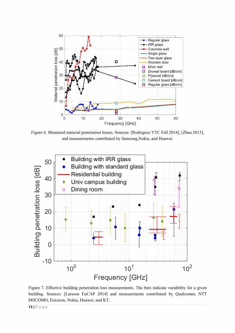
Materials such as concrete or brick have losses that increase rapidly with frequency. Figure 6
summarizes some recent measurements of material losses including those outlined in the Annex. The
loss trends with frequency are linear to a first order of approximation. Variations around the linear
trend can be understood from multiple reflections within the material or between different layers
which cause constructive or destructive interference depending on the frequency and incidence angle.
13 | P a g e
Figure 6. Measured material penetration losses. Sources: [Rodriguez VTC Fall 2014], [Zhao 2013],
and measurements contributed by Samsung,Nokia, and Huawei.
Figure 7. Effective building penetration loss measurements. The bars indicate variability for a given
building. Sources: [Larsson EuCAP 2014] and measurements contributed by Qualcomm, NTT
DOCOMO, Ericsson, Nokia, Huawei, and KT.

14 | P a g e
Typical building facades are composed of several materials, e.g. glass, concrete, metal, brick, wood,
etc. Propagation of radio waves into or out of a building will in most cases be a combination of
transmission paths through different materials, i.e. through windows and through the facade between
the windows. The exception could be when very narrow beams are used which only illuminates a
single material or when the indoor node is very close to the external wall. Thus, the effective
penetration loss can behave a bit differently than the single material loss. A number of recent
measurements of the effective penetration loss for close to perpendicular incidence angles are
summarized in Figure 7. As indicated by the error-bars available for some of the measurements, there
can be quite some variation even in a single building. The measurements can loosely be grouped into
two categories: a set of high penetration loss results for buildings constructed with IRR glass, and a
set of lower loss results for different buildings where regular glass has been used,
Increased penetration losses have been observed for more grazing incidence angles, resulting in up to
15-20 dB additional penetration loss in the worst case.
Propagation deeper into the building will also be associated with an additional loss due to internal
walls, furniture etc. This additional loss appears to be rather weakly frequency-dependent but rather
strongly dependent on the interior composition of the building. Observed losses over the 2-60 GHz
range of 0.2-2 dB/m.
4.4.2 Inside buildings
Measurements have been reported for penetration loss for various materials at 2.5, 28, and 60 GHz for
indoor scenarios [Rappaport Book2015] [Rappaport 2013] [And 2002] [Nie13] [ Zhao 2013]. For
easy comparisons, walls and drywalls were lumped into a common dataset and different types of clear
class were lumped into a common dataset with normalized penetration loss shown in Figure 8. It was
observed that clear glass has widely varying attenuation (20 dB/cm at 2.5 GHz, 3.5 dB/cm at 28 GHz,
and 11.3 dB/cm at 60 GHz). For mesh glass, penetration was observed to increase as a function of
frequency (24.1 dB/cm at 2.5 GHz and 31.9 dB/cm at 60 GHz), and a similar trend was observed with
whiteboard penetration increasing as frequency increased. At 28 GHz, indoor tinted glass resulted in a
penetration loss 24.5 dB/cm. Walls showed very little attenuation per cm of distance at 28 GHz (less
than 1 dB/cm).

15 | P a g e
Figure 8. 2.5 GHz, 28 GHz, and 60 GHz normalized material penetration losses from indoor
measurements with common types of glass and walls lumped into common datasets [Rappaport 2013]
[And2002][ Zhao 2013] [Nie 2013].
4.5 Blockage in all Environments
As the radio frequency increases, its propagation behaves more like optical propagation and may
become blocked by intervening objects. Typically, two categories of blockage are considered:
dynamic blockage and geometry-induced blockage. Dynamic blockage is caused by the moving
objects (i.e., cars, people) in the communication environment. The effect is transient additional loss on
the paths that intercept the moving object. Figure 9 shows such an example from 28 GHz
measurement done by Intel/Fraunhofer HHI in Berlin. In these experiments, time continuous
measurements were made with the transmitter and receiver on each side of the road that had on-off
traffic controlled by traffic light. Note that the time periods when the traffic light is red is clearly seen
in the figure as periods with little variation as the vehicles are static at that time. When the traffic light
is green, the blocking vehicles move through the transmission path at a rapid pace as is seen in the
figure. The variations seen when the light is red are explained by vehicles turning the corner to pass
between the transmitter and receiver. Figure 10 shows a blockage measurement at 28 GHz due to
passing by bus and lorry. The signal attenuation at LOS path is observed to be 8 dB – 30 dB. Signal
fluctuation is observed during the period of blockage perhaps due to windows in the bus and lorry.
The aggregated omni signal attenuation is observed to be around 10 dB – despite the high attenuation
on the LOS path, some of the NLOS paths can still go through. Figure 11 shows a blockage
measurement at 15 GHz by garbage truck [Ökvist 2016]. The signal was transmitted from two carriers,
each with 100 MHz bandwidth. The signal attenuation is observed to be 8 – 10 dB. A gap between
drivers compartment and trash bin can be observed, where temporal recovery of signal strength is
observed. Figure 12 shows a blockage measurement at 73.5 GHz by human movement. The
measurement setup is shown in Figure 13, where the transmitter and receiver are placed at 5 m apart

16 | P a g e
and 11 blocker bins are measured each separated by 0.5 m [MacCartney16]. The average LOS
blockage shadowing values across the blockage bins range from 22 dB to more than 40 dB. The
lowest shadowing value is achieved when the blocker is standing in the middle of the transmitter
and receiver. When the blocker moves closer to the transmitter or the receiver, the blockage
shadowing increases, This implicates that more NLOS paths are blocked when the blocker is at close
distance to the transmitter and receiver. Based on the above measurement results, we can observe that
blocking only happens in some directions, multipath from other directions probably not affected. The
effect of blockage can be modelled as additional shadow fading on the affected directions.
Figure 9 Example of dynamic blockage from a measurement snapshot at 28 GHz by Intel/Fraunhofer
HHI
Figure 10 blockage measurement at 28 GHz by distant bus + lorry by Intel/Fraunhofer HHI

17 | P a g e
Figure 11 Blockage measurement at 15GHz by garbage truck by Ericsson
Figure 12 Blockage measurement at 73.5 GHz by human being by NYU [MacCartney 2016]

18 | P a g e
Figure 13 measurement setup of human being blockage measurement in NYU [MacCartney 2016]
Geometry-induced blockage, on the other hand, is a static property of the environment. It is caused by
objects in the map environment that block the signal paths. The propagation channels in
geometry-induced blockage locations are dominated by diffraction and sometimes by diffuse
scattering. The effect is an exceptional additional loss beyond the normal path loss and shadow
fading. Figure 14 illustrates examples of diffraction-dominated and reflection-dominated regions in an
idealized scenario. As compared to shadow fading caused by reflections, diffraction-dominated
shadow fading could have different statistics (e.g., different mean, variance and coherence distance).
Tx
Diffraction Reg Reflection-
dominated Reg
LOS region
Figure 14 Example of diffraction-dominated and reflection-dominated regions (idealized scenario)

19 | P a g e
5 Channel Modelling Considerations
Table 1 summarizes a review of the 3GPP 3D channel model [3GPP TR36.873] capabilities. A plus
sign “+” means that the current 3GPP 3D channel model supports the requirement, or the necessary
changes are very simple. A minus sign “-” means that the current channel model does not support the
requirement. This evaluation is further split into two frequency ranges: below 6 GHz and above 6
GHz. Note that in the table, LSP stands for large-scale parameter.
Table 1. Channel Modelling Considerations
Attribute Requirement Below
6 GHz
Above
6 GHz
Improvement
addressed in
this white
paper
Comments
#1 Scenarios Support of new
scenarios such as
indoor office,
stadium, shopping
mall etc.
- - Current 3GPP
model supports
UMi and UMa
#2 Frequency
Range
0.5 GHz – 100 GHz
supported
+ - Current 3GPP
model 2 – 6 GHz
Consistency of
channel model
parameters
between different
frequency bands
- - E.g. shadowing,
angle of departure,
and in carrier
aggregation
#3 Bandwidth ~100 MHz BW for
below 6 GHz,
2 GHz BW for
above 6 GHz
+ -
#4 Spatial
Consistency
Spatial consistency
of LSPs with fixed
BS
+ - LSP map (2D or
3D)
Spatial consistency
of LSPs with
arbitrary Tx / Rx
locations (D2D /
V2V)
- - Complexity issue
(4D or 6D map)
Fair comparison of
different network
topologies
- -
Spatial consistency
of SSPs
- - Autocorrelation of
SSPs

20 | P a g e
UDN / MU
Consistency
- - Sharing of objects
/ clusters
Distributed
antennas and
extremely large
arrays
- -
Dynamic channel
(smooth evolution
of SSPs and LSPs)
- - Tx / Rx / scatterer
mobility
Possible methods
for modelling
varying DoDs and
DoAs are discussed
in the Appendix
#5 Large
Array Support
Spherical wave - - Also far field
spherical
High angular
resolution down to
1 degree
- - Realistic PAS?
Accurate modelling
of Laplacian PAS
- - 20 sinusoids
problem
Very large arrays
beyond
consistency
interval
- - Via spatial
consistency
modelling
#6
Dual-mobility
support (D2D,
V2V)
Dual Doppler + - Not yet done,
but should be easy
Dual angle of
arrival (AoA)
+ - Not yet done,
but should be easy
Dual Antenna
Pattern (mobile
antenna pattern at
both ends of the
link)
+ - Not yet done,
but should be easy
Arbitrary UE
height (e.g.
different floors)
- -
Spatially consistent
multi-dimensional
map
- - Complexity issue
(4D or 6D map)
#7 LOS
Probability
Spatially consistent
LOS probability /
LOS existence
- -

21 | P a g e
#8 Specular
Reflection
? - Important in mmW
#9 Path Loss Frequency
dependent path
loss model
+ -
Power scaling
(directive antennas
vs.
omnidirectional)
? -
Multiple NLOS
cases
? - Important in mmW
#10
Shadowing
Log-normal
shadowing
+ - Shadow fading
(SF) parameters
needed for high
frequency
Body shadowing - -
#11 Blockage Blockage modelling - -
#12 Cluster
definition
3GPP 3D cluster is
defined as fixed
delay and
Laplacian shape
angular spread.
+ - It is not
guaranteed that
the Laplacian
shape cluster is
valid for mmW.
#13 Drop
concept (block
stationarity)
APs and UEs are
dropped in some
manner (e.g.,
hexagonal grid for
3GPP)
+ - It is not sure if the
drop concept
works perfectly in
mmWave. Also it is
not clear how to
test beam tracking,
for instance.
#14 Accurate
LSP
Correlation
Consistent
correlation of LSPs
is needed.
- - The current 3GPP
model provides
different result
depending on the
order of
calculation
(autocorrelation,
cross-correlation)

22 | P a g e
#15 Number
of Paths
The number of
paths needs to be
accurate across
frequency.
+ - The current model
is based on low
frequency
measurements.
#16 Moving
Environment
Cars, people,
vegetation etc.
- -
#17 Diffuse
Propagation
Specular vs. diffuse
power ratio,
modelling of
diffuse scattering
+ - Most mmW
measurements
report specular
only despite the
fact that diffuse
exists
5.1 Support for a large frequency range
One of the outcomes of WRC-15 is that there will be studies of bands in the frequency range between
24.25 and 86 GHz for possible future IMT-2020 designation [ITU 238]. For the 3GPP studies, the
broader range of 6 GHz to 100 GHz should be studied for modelling purposes. Furthermore, as
mentioned in [3GPP RP-151606], possible implication of the new channel model on the existing 3D
channel model for below 6 GHz should also be considered. It is worth noting that the frequency range
of 3GPP 3D model is limited to LTE / LTE Advanced bands: “The applicable range of the 3D channel
model is at least for 2-3.5 GHz” [3GPP TR36.873]. Therefore a significant improvement is needed in
terms of frequency range for modelling tools.
In addition to the frequency range, the channel model should be frequency consistent, i.e. the
correlation of LSPs and SSPs between frequency bands should be realistically modelled, and the LOS
state and indoor state should not change randomly over frequency.
5.2 Support for high bandwidths
Many scenarios for 5G high frequency services postulate very high data rates up to several
gigabits/second for user services. Such high throughput communications will require channels of very
wide bandwidth (up to several gigahertz). The bands to be studied under the ITU-R Resolution [ITU
238] cover frequency bands up to 100 GHz (including 66 GHz – 76 GHz). The implication is that one
operator may be allocated multiple gigahertz wide channels for operation. Therefore, the channel
modelling should include support for scenarios with bandwidths up to several gigahertz. This implies
that the delay resolution of the modelled channel needs to be much improved compared to [3GPP
TR36.873] to produce realistic frequency domain characteristics over several GHz. This will likely
require modifications of the cluster distributions in delay and the sub-path distributions within
clusters.
5.3 Modelling of spatial consistency
The requirement of spatial consistency is probably the most challenging to meet with simple
extensions to the current “drop-based” models, as there are multiple aspects of the channel conditions,
including large-scale parameters and small-scale parameters, that would need to vary in a continuous
and realistic manner as a function of position. These conditions will include the LOS/NLOS state, the

23 | P a g e
indoor/outdoor state, and of course the parameters for the associated clusters of multipath components
characterized by angles, delays, and powers. Preferably the inclusion of spatial consistency should not
come at the cost of a high implementation or simulation complexity, and the channel statistics should
be maintained.
Three different approaches for introducing spatial consistency modelling will be outlined here. At this
point, no preference is given to any of the methods since they all have different benefits and
drawbacks.
5.3.1 Method using Spatially consistent random variables
In this approach, the spatial consistency of channel clusters are modelled in the 3GPP 3D channel
model [3GPP TR 36.873] by introducing spatial consistency to the channel cluster specific random
variables, LOS/NLOS and indoor/outdoor states.
1) Spatially consistent cluster specific random variables
The channel cluster specific random variables include:
a) Cluster specific random delay in step 5
b) Cluster specific shadowing in step 6
c) Cluster specific offset for AoD/AoA/ZoD/ZoA in step 7
d) Cluster specific sign for AoD/AoA/ZoD/ZoA in step 7
Among these cluster specific random variables, the first three are continuous random variables and are
made spatially consistent using the following method. The fourth variable is discrete and is generated
per drop instead of varying spatially to avoid discontinuous sign changes.
The spatially consistent random variables can be generated by interpolating i.i.d. random variables
deployed in the simulation area. this is a simulation-time-saving approximation to the
two-dimensional filtering with the autocorrelation function [Forkel et al. 2004].For example in Figure
15, one spatially consistent uniform distributed random variable can be generated by dropping four
complex normal distributed i.i.d. random variables on four vertex of one grid with dcorr (e.g. dcorr=50)
de-correlation distance and interpolated using these i.i.d. random variables. The de-correlation
distance could be a scenario specific parameter. In order to save simulation complexity, a grid may be
generated only if there are actual users dropped within the grid area.
Figure 15 Example of generating one spatially consistent random variable.
dcorr=50 Y1,1~CN(0, 0,1)
x
y
Y(x, y)
Y0,1~CN(0, 0,1)
Y0,0~CN(0, 0,1)Y1,0~CN(0, 0,1)

24 | P a g e
Assuming Y0,0, Y0,1, Y1,0, Y1,1 are the i.i.d. complex normal random numbers generated on the four
vertex of one grid, the complex normal number Yx,y at position (x, y) can be interpolated as equation
(x.1):
𝑌(𝑥,𝑦) = √1 − 𝑦/𝑑𝑐𝑜𝑟𝑟(√1 − 𝑥/𝑑𝑐𝑜𝑟𝑟𝑌0,0 +√𝑥/𝑑𝑐𝑜𝑟𝑟𝑌1,0) + √𝑦/𝑑𝑐𝑜𝑟𝑟(√1 − 𝑥/𝑑𝑐𝑜𝑟𝑟𝑌0,1 +
√𝑥/𝑑𝑐𝑜𝑟𝑟𝑌1,1) (x.1)
One uniform random number can be generated using the phase of the interpolated complex normal
random number as equation (x.2):
𝑋𝑛 = |𝑎𝑛𝑔𝑙𝑒(𝑌(𝑥,𝑦))/𝜋| (x.2)
where | | operation ensures there is no abrupt change of the interpolated random number 𝑋𝑛
between 0 and 1 along a trajectory. This will be desired when the uniform random number is used to
generate cluster specific random delay in step 5 because otherwise the delay of one cluster could
change between infinity to zero along a trajectory.
The spatially consistent normal distributed random variable can be generated by dropping normal
distributed random variables on the vertex of one grid and interpolated among the random variables.
The cluster specific random variables should be applied to one cluster before clusters are sorted based
on its random delay.
This method can be extended to additional dimensions, e.g. temporal/frequency, to generate
spatial/temporal/frequency consistent random numbers.
2) Spatially consistent LOS/NLOS state
Variant 1: The spatially consistent LOS/NLOS state can be generated by comparing a spatially
consistent uniform distributed random number with the LOS probability at a given position. Soft
LOS/NLOS state can be generated by filtering the binary LOS/NLOS state over space. Figure 16
gives one example of generating the soft LOS/NLOS state and its effect. The soft LOS/NLOS state at
a given position is calculated using the average of nine binary LOS/NLOS states at nine positions on
the square centred by the position of interests. The middle plot depicts the spatially consistent binary
LOS/NLOS state with 50 meter de-correlation distance. The right plot depicts the spatially consistent
soft LOS/NLOS state with 50 meter de-correlation distance and 1 meter transition distance.
Figure 16 Example of generating one soft LOS/NLOS state.
Variant 2: In this variant, a spatially consistent Gaussian number G with autocorrelation distance dLOS
is generated. This is combined with a threshold value F determined via
dtransition=2
LoSx,y=1dtransition/2=1
dtransition/2=1
LoSx,y-1=1 LoSx+1,y-1=1LoSx-1,y-1=1
LoSx+1,y=1LoSx-1,y=1
LoSx+1,y+1=1LoSx-1,y+1=1 LoSx,y+1=1
Soft_LoSx,y=7/9

25 | P a g e
𝐹(𝑑) = √2𝑒𝑟𝑓−1(2𝑃𝐿𝑂𝑆(𝑑) − 1)
Here 𝑑 is the distance and 𝑃𝐿𝑂𝑆(𝑑) is the LOS probability function. The soft LOS state is
determined by a function approximating knife-edge diffraction:
𝐿𝑂𝑆𝑠𝑜𝑓𝑡 =1
2+1
𝜋arctan(√
𝑑𝐿𝑂𝑆𝜆
(𝐺 + 𝐹))
An examples of the soft LOS/NLOS state using this method is given in Figure 17. Note that the
transition becomes more rapid with increasing frequency and that the transition will behave similarly
as in some of the reported blocking measurements in the Annex.
An alternative implementation for spatially consistent LOS/NLOS, based on the concept of visibility
regions, has been proposed in the COST 259 model [Molisch et al. 2006, Asplund et al. 2006] and its
successors.
Figure 17 Example of spatially consistent soft LOS state using second variant (left) and a transition from
NLOS to LOS (right)
3) Spatially consistent indoor/outdoor state
Spatially consistent indoor/outdoor state can be generated by comparing a spatially consistent uniform
distributed random number with the indoor/outdoor probability at a given position. Similarly as soft
LOS/NLOS state, soft indoor/outdoor state can be introduced by filtering binary indoor/outdoor state
over space. Alternatively, transitions between the outdoor and indoor states can be avoided through
modifications of the mobility model if this would be more desirable.
4) Spatially consistent path loss
Based on the soft LOS/NLOS and soft indoor/outdoor states, spatially consistent path loss can be
defined using the soft LOS/NLOS and indoor/outdoor states as equation (x.3).
𝑃𝐿(𝐿𝑂𝑆𝑠𝑜𝑓𝑡 , 𝐼𝑁𝐷𝑂𝑂𝑅𝑠𝑜𝑓𝑡) = 𝑃𝐿𝐿𝑂𝑆 ∗ 𝐿𝑂𝑆𝑠𝑜𝑓𝑡 + 𝑃𝐿𝑁𝐿𝑂𝑆 ∗ (1 − 𝐿𝑂𝑆𝑠𝑜𝑓𝑡) + 𝐼𝑁𝐷𝑂𝑂𝑅𝑠𝑜𝑓𝑡 ∗
𝑃𝑒𝑛𝑒𝑟𝑎𝑡𝑖𝑜𝑛𝐿𝑜𝑠𝑠 (x.3)
Since penetration loss is a function of indoor distance, we can make penetration loss to be spatially
consistent to have spatially consistent path loss for indoor state.
5) Spatially consistent small scale fading channels
Based on the soft LOS/NLOS and indoor/outdoor states, the spatially consistent small scale fading
channel matrix can be generated using equation (x.4).

26 | P a g e
𝐻(𝐿𝑂𝑆𝑠𝑜𝑓𝑡 , 𝐼𝑁𝐷𝑂𝑂𝑅𝑠𝑜𝑓𝑡) = √1 − 𝐼𝑁𝐷𝑂𝑂𝑅𝑠𝑜𝑓𝑡(𝐻𝑜𝑢𝑡𝑑𝑜𝑜𝑟_𝐿𝑂𝑆 ∗ √𝐿𝑂𝑆𝑠𝑜𝑓𝑡 +𝐻𝑜𝑢𝑡𝑑𝑜𝑜𝑟_𝑁𝐿𝑂𝑆 ∗
√1 − 𝐿𝑂𝑆𝑠𝑜𝑓𝑡) + √𝐼𝑁𝐷𝑂𝑂𝑅𝑠𝑜𝑓𝑡 ∗ 𝐻𝐼𝑛𝑑𝑜𝑜𝑟 (x.4)
To summarize, this method can be implemented with a similar complexity as the spatially consistent
large-scale parameters which are already a part of most drop-based models such as [3GPP TR36.873].
Smooth variations of angles and delays will be induced, although these will not fully resemble
variations seen in measurements. Instead, they will tend to be a bit too smooth and synthetic, and the
rate of variations can sometimes be unphysically high, This method will maintain the channel
statistics which is a very desirable characteristic.
Another important aspect of obtaining spatially consistent pathloss is to describe the fact that different
streets/areas can experience different pathloss coefficients, in particular in microcells; for further
discussion we refer to [Molisch et al. 2016].
5.3.2 Geometric Stochastic Approach
Spatial consistency means that channel realizations including large-scale parameters (LSPs) and
small-scale parameters (SSPs) would need to vary in a continuous and realistic manner as a function
of position in geometry. Two features of spatial consistency are important. Firstly, user equipments
(UEs) sharing similar locations should have correlated LSPs, and the LSPs should be crucially
dependent on UE’s position instead of random allocation in each drop as done in 3GPP SCM.
Moreover, the path loss including shadow fading should vary smoothly as UE moves in geometry,
even in a drop duration. This is particularly important to the evaluation of multiuser MIMO or
multiuser beam-forming techniques. Secondly, SSPs in a drop (e.g. angle, power, and delay) should
be dynamically changing with position. More accurately, the new model realizes time-variant angles
and cluster death and birth as UE is moving which is important to evaluate mobility and beam
tracking for 5G communications.
Geometry stochastic approach for spatial consistency might be the suitable solution to extend 3GPP
SCM with small changes in sense of backward compatibility; note that other models such as COST
273/2100 explicitly model reflection points geometrically and thus do not need the transformations
shown here.. The modified procedures for the new model based on 3GPP SCM [1] is summarized as
follows.
- 3GPP SCM step 1 and 2: Pre-compute the LSPs for each grid, grid shape can be rectangular
with side length of spatial consistent distance. See item-C.
- 3GPP SCM step 3 and 4: Every UE takes the LSPs of the grid that the UE locates. See
item-C. Calculate the path loss based on UE’s position. See item-A and item-B.
- 3GPP SCM step 5: Add the decision of cluster birth and death. If yes, take the procedure of
cluster birth and death in item-E.
- 3GPP SCM step 11: Update the angles based on item-D at the beginning of the step.
A. Geometry position
Geometry positions of UE, scatters, and BS are the fundamental information of SCM, and are fixed in
a drop. Actually the position of UE is time variant as UE is moving. Suppose the moving speed of UE

27 | P a g e
is v and moving direction is v in global coordination system (GCS), the position of UE at time t is
given by
UE
vAoDZoD
vAoDZoD
UE
h
ttvtd
ttvtd
tX )sin()()sin()sin()(
)cos()()cos()sin()(
)( 00
00
,
where 0td is the distance between BS and UE at previous time t0. Notice that the time interval
0tt can be a sub-frame duration as used in 3GPP.
B. Time-variant Path loss
The path loss is crucially depending on the position of UE or distance between BS and UE. Since
BS’s position is fixed at XBS = (0, 0, hBS)T, the distance between BS and UE at time t is
)()( tXXtd UEBS .
With the path loss model for above 6 GHz or 3GPP path model for sub-6GHz, the path loss at time t
can be updated accordingly. The correlated shadow fading in different positions are discussed in
section 7.2.1 in 3GPP TR 36.873. The correlated shadow fading is given by
2
2
1 .1.)( FFdF ,
where )/exp( cordd , dcor is the correlation distance of shadow fading, F1 and F2 are the shadow
fading allocated in two neighbouring grids.
C. Position-based Large-scale Parameters (LSPs)
3GPP SCM allocate LSPs randomly for each UE. Two UEs may have much different LSPs although
they are close in locations. The fact is the LSPs of the two UEs should be similar which leads to
channel impulse response with high correlation. In order to circulate the problem, we divide each cell
under a BS’s coverage into multiple grids. Each grid is spatial consistent in sense of large-scale fading
characteristics. Each grid is configured with a set of LSPs following the given probability density
function defined in 3GPP SCM. Grid centre is assumed as the location in calculating LSPs. In the step
to generate the LSPs for a UE channel, it firstly checks which grid the UE locates, and then take the
LSPs of the corresponding grid to the UE channel. In this way, UE sharing the same grid will have the
same LSPs.

28 | P a g e
Set scenario,
network layout and
antenna parameters
Get propagation
condition (NLOS/
LOS)Calculate pathloss
Get correlated large
scale parameters
(DS, AS, SF, K)
General parameters:
Small scale parameters:
Set scenario,
network layout and
Grid parameters
Assign propagation
condition (NLOS/
LOS) for every grid
Generate correlated
large scale
parameters (DS,
AS, SF, K) for every
grid
Save the Grid-
based LSP table
Grid-based LSPs
Fig. 1 LSPs generation procedure
Fig. 1 illustrates the procedure to generate LSPs where red texts are the new steps based on 3GPP
TR 36.873. Notice that the grid-based LSPs are calculated only once and are saved as a table. Most
LSPs of UEs are taken from the table. Thus, the computational complexity of LSPs is lower than
3GPP SCM.
D. Time-variant Angle
Variant angles are introduced for each ray including azimuth angle of departure and arrival (AoD,
AoA) and zenith angle of departure and arrival (ZoD, ZoA) in [Wang2015]. Since UE’s position at
time t is available, the angles can be updated with transmitter and receiver information in the global
coordination system (GCS). Linear approximation is an efficient way to reduce complexity with
acceptable errors. The linear method for variant angles are generally formulated as [Wang 2015]
)()()( 0,,0,,,, ttStt AnglemnAnglemnAnglemn ,
where the sub-index “Angle” represents AoA, AoD, ZoA, or ZoD in SCM. AnglemnS ,,
is the slope which
describes the changing ratio of time-varying angles. For LOS cluster, the expression of AoD and ZoD
slopes are given by [Wang2015]
))(cos(/)(
))(cos(
0
0
thh
tvSS
ZODUEBS
AODvZOAZOD
,
))(tan()(
))(sin(
0
0
thh
tvSS
ZODUEBS
AODvAOAAOD
.
For NLOS cluster with one reflection ray, the model can be simplified by introducing a virtual UE
which is the mirror image of UE based on the reflection surface. The simplified slopes in NLOS
channel are given by [Wang2015]
))(cos(/)(
))(sin(
0
0\
thh
tvSS
ZoDUEBS
RSAODvZoAZoD
,
))(tan()(
))(cos(
0
0
thh
tvSS
ZoDUEBS
RSAoDv
AoAAoD
,

29 | P a g e
where RS is the angle of the reflection surface and it can be deduced from the initial AoD and
AoA .
E. Cluster Birth and Death
Cluster birth and death are assumed to happen at the same time in order to keep a fixed number
clusters as defined in 3GPP SCM. Scatters are assumed to be independent with each other. In this
sense, cluster birth and death can be modeled with Poisson process if looking the rate of cluster
birth/death in time. Accurately, the cluster birth/death will happen at time t with the probability
))(exp(1)Pr( 0ttt c ,
where t0 is the previous time that cluster birth/death happened. The model has single parameter λc
which represents the average number of cluster birth/death per second, and hence is very simple in
channel simulations. The single parameter λc is essentially depending on the number of birth/death in
a spatial consistency distance and UE moving speed. For cluster death, the cluster selection can be
based on the cluster power from weak to strong since weak cluster is easy to change [WINNER]. For
cluster birth, new cluster can copy the cluster (power, delay, and angles) from nearest grid. The
priority of cluster selection is based on the cluster power from weak to strong. When UE is moving to
the neighbouring grid, the clusters will be replaced by the new clusters of neighbouring grid gradually
and hence keep spatial consistency in sense cluster.
5.3.3 Method using geometric locations of clusters (Grid-based GSCM, GGSCM)
According to the drop concept of the conventional GSCMs (SCM, WINNER, IMT-Advanced, 3GPP
3D, etc.), the receivers (Rx’s) are located randomly and the propagation parameters are randomly
drawn from the pre-defined probability distributions. The channel is assumed to be stationary along a
short distance (segment), but this assumption does not hold for longer distances, therefore the
parameters need to be re-calculated (new drop/segment). This approach is called as block-stationary
modelling in which large scale (LS) and small scale (SS) parameters are fixed during the segment and
fully different between the segments. The transition from a segment to another provides a rapid
change of channel model parameters thus the channel is discontinuous. To improve the reality and
time evolution, it is possible to interpolate between the segments. However, it is difficult to ensure
spatial consistency especially between nearby users in multi-user case. Therefore, a new method
(partly based on [METIS_D1.2]) is proposed and drafted in the following.
In the method, called Grid-based GSCM (GGSCM), cluster and path angles and delays are translated
into geometrical positions (x, y) of the corresponding scatterers, see Figure 18. The benefit is that the
cluster and path evolution in delay and angle can be naturally traced and will have very realistic
variations.

30 | P a g e
Figure 18 Clusters are translated into geometric positions
This method needs to be complemented with some birth/death process to maintain uniformity of
clusters during movement. An example clarifies this discussion. Let us consider a case of three users:
A, B, and C (Figure 19). Users A and C are far away from each other. They may assume independent
clusters. However, the users A and B are located nearby. The current 3GPP-3D model assumes
independent small scale parameters (SSPs), which lead to non-physical situation, and too optimistic
MU-MIMO throughput evaluations. Figure 20 illustrates the thinking of spatially consistent case in
which all or some of the clusters are shared between nearby users.
Figure 19. The problem of independent clusters of nearby users (current GSCM).
Figure 20. Shared clusters (necessary improvement).
Figure 21 depicts the situation in which a high number of users are “dropped” onto a 2-dimensional
map. Each user has a ring around, and the radius of that ring is equal to the correlation distance (or
A
C
B
A
C
B

31 | P a g e
stationarity interval). If another user is located inside that ring, the spatial consistency has to be taken
into account. Otherwise, current method of random SSPs is acceptable.
Figure 21. Dropping of users.
In the case of nearby users, the clusters should be interpolated between the users. User B takes the N
strongest clusters (N is the number of clusters defined per scenario).
Figure 22. User centric selection of clusters.
The interpolation can be done along a route of based on a pre-defined “grid” (Grid based GSCM,
GGSCM). In the GGSCM approach a discrete two-dimensional map of possible Rx locations is
defined. Instead of drawing LSPs and SSPs for the actual user locations, the cluster parameters are
drawn for every grid point. Then the cluster parameters for the actual Rx locations are interpolated
between four nearest grid points. The grid can be intuitively understood as a drop in which the
distance between two adjacent users is constant in x and y dimensions. The drops are independent
between the GPs, i.e., LSPs and SSPs are randomly drawn from the pre-defined distributions (similar
to the legacy GSCM).
Independent
User,independent clusters
Correlation distance
These users share some clusters
A
C
B

32 | P a g e
Figure 23. Grid model (GGSCM): Calculate new cluster information at each grid point. Interpolate
clusters between the four grid points.
The locations of the clusters have to be defined in (x, y) or (x, y, z) coordinates. The maximum
distance between Rx (or Tx) and the cluster location is determined from the geometry of Rx and Tx
locations, AoA, AoD, and delay. This geometry is an ellipse with focal points at Rx and Tx locations,
and the major axis equals to the delay multiplied by the speed of light. In the case of single bounce,
the cluster is located on the locus of an ellipse defined by AoA, AoD, and delay (see Figure 24, SBC,
single bounce cluster). In the case of multi-bounce, the same locus defines upper bound of the
distance of the cluster, i.e. the cluster can be anywhere in the segment between Tx (or Rx) and the
locus (see Figure 24, FBC/LBC, first/last bounce cluster). A distribution for that cluster location could
be uniform between the two ends of said segment. Because the AoA, AoD, and delay are randomly
drawn in the GSCM, most likely the geometry of these three parameters does not fit to the ellipse.
Thus the 50% of the cluster locations may be based on Rx-side cluster parameters and another 50%
based on Tx-side cluster parameters.
Figure 24. Location of a cluster.
Tx Rx
AoD AoA
d1 d2
cddd 21
FBC
LBC
SBC
33 | P a g e
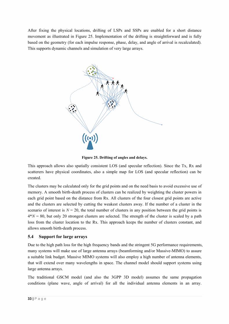
After fixing the physical locations, drifting of LSPs and SSPs are enabled for a short distance
movement as illustrated in Figure 25. Implementation of the drifting is straightforward and is fully
based on the geometry (for each impulse response, phase, delay, and angle of arrival is recalculated).
This supports dynamic channels and simulation of very large arrays.
Figure 25. Drifting of angles and delays.
This approach allows also spatially consistent LOS (and specular reflection). Since the Tx, Rx and
scatterers have physical coordinates, also a simple map for LOS (and specular reflection) can be
created.
The clusters may be calculated only for the grid points and on the need basis to avoid excessive use of
memory. A smooth birth-death process of clusters can be realized by weighting the cluster powers in
each grid point based on the distance from Rx. All clusters of the four closest grid points are active
and the clusters are selected by cutting the weakest clusters away. If the number of a cluster in the
scenario of interest is N = 20, the total number of clusters in any position between the grid points is
4*N = 80, but only 20 strongest clusters are selected. The strength of the cluster is scaled by a path
loss from the cluster location to the Rx. This approach keeps the number of clusters constant, and
allows smooth birth-death process.
5.4 Support for large arrays
Due to the high path loss for the high frequency bands and the stringent 5G performance requirements,
many systems will make use of large antenna arrays (beamforming and/or Massive-MIMO) to assure
a suitable link budget. Massive MIMO systems will also employ a high number of antenna elements,
that will extend over many wavelengths in space. The channel model should support systems using
large antenna arrays.
The traditional GSCM model (and also the 3GPP 3D model) assumes the same propagation
conditions (plane wave, angle of arrival) for all the individual antenna elements in an array.

34 | P a g e
However this approximation becomes inaccurate when the number of antenna elements is large and
may cover an area of many wavelengths.
While the far field criterion is often seen as guaranteeing plane waves, unfortunately this is not always
true for large antenna arrays. Spherical waves may need to be taken into account for larger distances
and for the short ranges expected for the millimetre wave communications links.
The phase error from the centre of the antenna array to the most distant antenna element can be easily
calculated from the geometry. With values 1λ < D < 10λ, the error is within 22.0°…22.5°. For beam
forming and interference cancellation, the modelling error should be less than, say << 5°. Therefore,
the plane wave assumption is true only if the distance is larger than 4d (to be on the safe side, 8d is
recommended). The far field distance d for a massive MIMO antenna for the millimetre wave
frequencies of interest would normally be between 5 to 10 meters, implying that the minimum
antenna to cluster distance to safely utilize planar wavefront modelling would be in the range 40 to 80
meters, which is beyond the deployment scenarios many cases. As a consequence, spherical wave
modelling may become important for 5G channel modelling with very large array manifolds.
The 3GPP 3D model assumes a Laplacian power angular spectrum (PAS) may be adequately
modelled by 20 equal amplitude sinusoids. This approximation may be sufficient for small arrays.
However, large arrays require accurate angular resolution, otherwise they will see each sinusoid as a
separate specular wave, which is non-physical. This problem was studied in the contribution [Anite
Telecoms 2014] and in the reference [W. Fan 2015].
In the 3GPP 3D channel model, the pairing between azimuth and elevation angles is done randomly,
i.e. each azimuth angle is randomly paired with an elevation angle, and the total number of sub-rays is
still 20. Different realizations provide different pairing of elevation and azimuth angles. Figure 26
shows an example of random pairing. The projection to azimuth or elevation plane provides the
Laplacian shape, but the projections to other planes do not necessarily correspond. This causes a
correlation error in the order of 0.11 … 0.15 (absolute values) [Anite Telecoms 2014].
Figure 26 Random pairing of azimuth and elevation angles.
-50 -40 -30 -20 -10 0 10 20 30 40 50-20
-10
0
10
20
Power Angle spectrum
Azimuth [unit:degree]
Ele
va
tio
n [u
nit:d
eg
ree
]
-50 0 500
0.01
0.02
0.03
0.04
0.05
Azimuth [unit:degree]
Po
we
r [u
nit:d
eg
ree
]
-20 -10 0 10 200
0.01
0.02
0.03
0.04
0.05
Elevation [unit:degree]
Po
we
r [u
nit:d
eg
ree
]
35 | P a g e
In addition to the spherical wave effect and other alignment problems, very large arrays may see
different propagation effects between the different elements of the array. While the minimum size of
an extremely large array is not well defined, one may say that an array becomes “large” when it is
larger than the consistency interval (or stationarity interval or correlation distance). The correlation
distance of large scale parameters varies significantly depending on the details of the environment.
For example, in WINNER II it varies from 0.5 to 120 m. Within these distances, all small scale
parameters such as angle of arrival, delay, Doppler, polarization, may be different across the array.
Also large scale parameters such as shadowing may affect only a sub-set of antenna elements in the
array, as has been observed in [Gao et al. 2015]. This is also likely the case with distributed antennas
and cooperative networks. The existing 3GPP 3D channel model assumes the same propagation
effects across the entire antenna array. This may not be the case for many of the future deployment
scenarios.
5.5 Dual mobility support
Dual mobility in the D2D and V2V scenarios causes different Doppler models, different spatial
correlation of large-scale and small-scale parameters than in the conventional cellular case. The
conventional cellular models presume at least one end of the radio link is fixed (usually the base
station). The corresponding Doppler spectrum and characteristic small scale fading distribution have
been modelled in particular for car-to-car communications, see, e.g., [Zajic and Stuber 1998], but
were considered outside the scope of the current work. To allow modelling for D2D and V2V 5G
scenarios, in which both ends of the link may be in motion and experience independent fading,
Doppler shift and channel conditions further additions to the channel models are required to
accommodate these parameters.
5.6 Dynamic blockage modelling
The dynamic blockage could be modelled as additional shadow fading on certain channel
directions. Assuming the distance between the blocker and transmitter is much farther away than the
distance between the blocker and receiver, the blocking effect can be applied to channel receiving
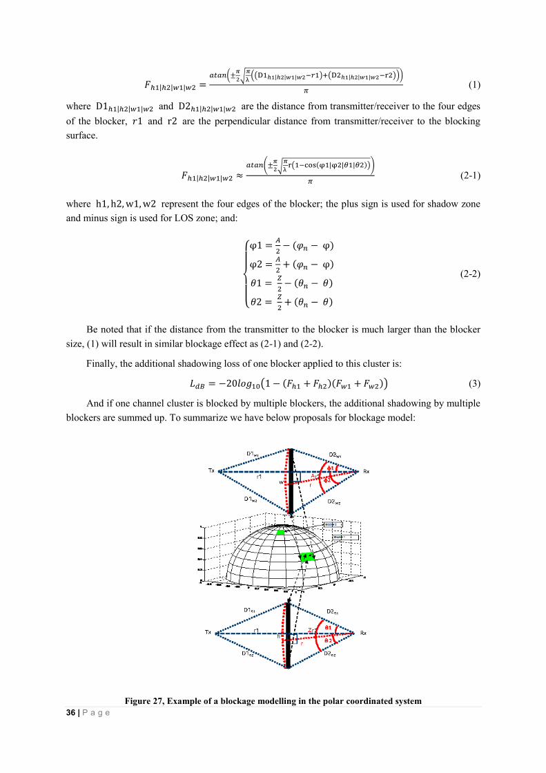
directions for simplicity. An example of two blockers is illustrated in Figure 27. Assume the position
of receiver is in the origin, we can describe one blocker in Cartesian/polar coordinate system using
below parameters:
1) Centre of the blocker (φ, θ, r), where φ, θ, r represent the azimuth angle, zenith angle, and
radius of the centre of the blocker
2) Azimuth angular span of the blocker (AoA span) A ≈ 𝑤/𝑟, where 𝑤 is the width of the
assumed rectangular blocking surface
3) Zenith angular span of the block (ZoA span) Z ≈ ℎ/𝑟, where ℎ is the height of the assumed
rectangular blocking surface
Assume the AoA/ZoA of one channel cluster is (𝜑𝑛, θ𝑛). The blockage effect for this cluster is
modelled if the |𝜑𝑛 − φ| < 𝐴 and |𝜃𝑛 − 𝜃| < 𝑍, and the blockage effect of one edge of the blocker
is modelled using a knife edge diffraction model for the four edges of the blocker as (1) in Cartesian
coordinate system or (2-1) and (2-2) in polar coordinate system:
36 | P a g e
𝐹ℎ1|ℎ2|𝑤1|𝑤2 =𝑎𝑡𝑎𝑛(±
𝜋
2√𝜋
λ ((D1ℎ1|ℎ2|𝑤1|𝑤2−𝑟1)+(D2ℎ1|ℎ2|𝑤1|𝑤2−r2)))
𝜋 (1)
where D1ℎ1|ℎ2|𝑤1|𝑤2 and D2ℎ1|ℎ2|𝑤1|𝑤2 are the distance from transmitter/receiver to the four edges
of the blocker, 𝑟1 and r2 are the perpendicular distance from transmitter/receiver to the blocking
surface.
𝐹ℎ1|ℎ2|𝑤1|𝑤2 ≈𝑎𝑡𝑎𝑛(±
𝜋
2√𝜋
λ r(1−cos(φ1|φ2|𝜃1|𝜃2)))
𝜋 (2-1)
where h1, h2,w1,w2 represent the four edges of the blocker; the plus sign is used for shadow zone
and minus sign is used for LOS zone; and:
{
φ1 =
𝐴
2− (𝜑𝑛 − φ)
φ2 =𝐴
2+ (𝜑𝑛 − φ)
𝜃1 = 𝑍
2− (𝜃𝑛 − 𝜃)
𝜃2 = 𝑍
2+ (𝜃𝑛 − 𝜃)
(2-2)
Be noted that if the distance from the transmitter to the blocker is much larger than the blocker
size, (1) will result in similar blockage effect as (2-1) and (2-2).
Finally, the additional shadowing loss of one blocker applied to this cluster is:
𝐿𝑑𝐵 = −20𝑙𝑜𝑔10(1 − (𝐹ℎ1 + 𝐹ℎ2)(𝐹𝑤1 + 𝐹𝑤2)) (3)
And if one channel cluster is blocked by multiple blockers, the additional shadowing by multiple
blockers are summed up. To summarize we have below proposals for blockage model:
Figure 27, Example of a blockage modelling in the polar coordinated system

37 | P a g e
For single link simulation, we can define blocker trajectory, size and distance based on
experiences either in Cartesian coordinate or polar coordinate systems. And the blocker size/distance
is deterministic in the simulations.
For full system level simulation, we can fix the blocker distance and randomly generate the azimuth
centre of the blocker using two uniformly distributed random variables 𝑢1, 𝑢2~𝑈(0,1), and the
centre of the blocker (φ, θ, r) = (2π𝑢1,π
2−π𝑢2
4, 2). The random variables 𝑢1 can be generated with
spatial/temporal consistency according to section 5.3.1 with correlation distance d𝑐𝑜𝑟𝑟 and
correlation time t𝑐𝑜𝑟𝑟 to model the blocker movement around the receiver in the azimuth dimension.
For example, d𝑐𝑜𝑟𝑟 = 50m and t𝑐𝑜𝑟𝑟 =𝜋
2r 𝑣⁄ . For random variable 𝑢2, it can be generated per drop
with spatial consistency. Thus the blocker does not move in the zenith dimension but two near-by
receivers still observe correlated blockege effect. Table 2 gives some configuration examples for the
blocker. The moving speed in system level is the mean moving speed of the blocker. The
instantaneous moving speed around a paticular receiver is statistically distributed.
For multiple blockers, each blocker can be configured with one blocker specific parameter sets.
Table 2 Typical configuration of blocker
Typical set of screens Screen dimensions
Indoor;
Outdoor
Human Cartesian: w=0.3m; h=1.7m; r = 2m; v=3km/h
Polar: A=0.15rad; Z = 0.85rad; r = 2m;
vp=0.42rad/s; tcorr=3.77s; dcorr=50m (outdoor);
dcorr=5m (indoor)
Outdoor Vehicle Cartesian: w=4.8m; h=1.4m; r = 10m; v =
30km/h
Polar: A=0.48rad; Z = 0.14rad; r = 10m;
vp=0.83rad/s; tcorr=1.88s; dcorr=50m
In Figure 28, this model is compared to measurement results for blocking by a passing garbage truck.
The truck has been modelled by two rectangular screens with sizes according to the sizes of the
drivers compartment and container, and the trajectory to the screens has been matched to the
trajectory of the truck. The only fitted model parameters are the speed of the truck (25 km/h) and the
K-factor in the channel (9 dB). As can be seen, the model reproduces the measured signal strength
drops and transitions exceptionally well.

38 | P a g e
Figure 28 Comparison between the proposed blocking model and measurements [Ökvist 2016]
5.7 Foliage loss
Measurements and modelling of foliage loss at higher frequencies can be found in [Schwering
1988],[Chavero 1999],[Rappaport ICC 2015],[ ITU-R P.833]. The loss increases with frequency and
penetration depth through the foliage. Modelling approaches such as [ITU-R P.833] can also account
for contributions from diffracted, ground-reflected and scattered waves. it is important not to account
for such losses twice in the channel model. In a stochastic path loss model the model is parameterized
using measurements in the scenarios of interest. In the UMa and UMi case this will include path loss
measurements in urban areas which often include trees and other vegetation. Thus, in a stochastic path
loss model the effect of the foliage is already included. It is therefore unnecessary to add an explicit
foliage loss model.
5.8 Atmospheric losses
In the UMa and UMi scenarios, the link distances could potentially be up to hundreds of meters and
interference may need to be modelled from transmitters that are up to a few kilometres distant. The
path loss model as a function of frequency will be a key component of the channel model. It is known
that atmospheric losses can become significant at higher frequencies and longer ranges. Figure 29
illustrates the measured atmospheric effects for normal and dry air compiled for the ITU. These are
expressed in terms of dB/km of path length. It can be seen that for the mmWave bands below about
100 GHz, the attenuation is dominated by the oxygen absorption peak at about 60 GHz. This peak is
about 15 dB/km or about 0.015 dB/metre. For the other frequencies below 100 GHz, the absorption is
about ten times less (or 0.001 dB/metre). In dry air the loss is much lower. For distances of tens of

39 | P a g e
meters in the InH and UMi these losses are not significant compared to other effects of the
environment (e.g. clutter and buildings). For 100+ metre ranges in the UMa scenario the 1.5 dB loss is
of small consequence compared to other effects.
Figure 29 Attenuation by atmospheric gases in the 0-1000 GHz range. Source: Rec ITU-R P.676-9
(02/2012) Attenuation by atmospheric gases
Figure 30 illustrates the measured rain attenuation for various rain-rates compiled for the ITU. These
are expressed in terms of dB/km of path length. Rainfall is not a consideration in the InH scenario
(indoors). For the outdoor scenarios, at 100 metre path lengths, the rainfall would cause less than 0.4,
0.8 or 2.0 dB loss for signals close to 100 GHz [Rappaport 2015]. As the average rain-rate is less than
the peak, the average loss would be somewhat less and also less for lower frequencies. In periods of
heavy rain the path loss may also be accompanied by scattering from the raindrops.
Figure 30 Rain attenuation for different rain intensities. Source: Rec ITU-R P.838-2 Specific attenuation
model for rain for use in prediction methods
0 100 200 300 4000
5
10
15
20
25
Frequency [GHz]
Rain
attenuation [dB
/km
]
50 mm/h
15 mm/h
5 mm/h

40 | P a g e
Overall, in most InH, UMi and UMa scenarios the effects of atmospheric loss and rainfall will be
insignificant compared to other factors of the environmental. For scenario deployments in the 100
metre range they may be worthwhile taking into account.
Since the attenuation due to water vapour will be insignificant for the typical link distances in the
considered scenarios is doesn’t seem necessary to model water vapour attenuation. While rain
attenuation could become significant for longer link distances and at higher frequencies, it will be
very rare with rain heavy enough to impact the shorter link distances that will be applicable in the
agreed scenarios. In typical 3GPP RAN1 simulations the time variability of the link quality is not
modelled, unlike the ITU sharing and coexistence studies where worst case interference conditions
have a higher importance. Therefore modelling of rain attenuation may be optional and only applied
to sharing and coexistence studies.
Oxygen absorption may become significant around the 60 GHz peak as shown in Figure 29. The
effect on the path loss can easily be accounted for using known models such as given by Rec ITU-R
P.676 [ITU-R P.676]. However, there is a secondary effect that may result in noticeable reductions of
delay and angular spread. This reduction is caused by the multipath components having longer path
length than the direct path and will suffer a slightly greater oxygen absorption. In order to have a joint
model parameterization over the full frequency range at longer ranges, it is proposed that
measurements of e.g. channel impulse responses are compensated for the oxygen absorption loss at
different delays. An example of the path loss and delay spread results before and after such
compensation is shown in [R1-160846]. By this procedure it is possible to characterize the
frequency-dependence of the channel dispersion without the notch-like effect near the oxygen peak
disrupting any smoother trends. This process means that the oxygen loss should be applied in a
separate modelling step. This can be done by attenuating each cluster (path) in the generated channel
impulse response by a loss 𝛼 ⋅ 𝑐 ⋅ 𝜏𝑛 [dB] where 𝛼 [dB/m] is the oxygen loss, c [m/s] is the speed of
light, and 𝜏𝑛 [s] is the cluster (path) delay.
41 | P a g e
6 Pathloss, Shadow Fading, LOS and Blockage Modelling
6.1 LOS probability
The definition of LOS used in this white paper is discussed in this sub-section together with other
LOS models. The LOS state is here determined by a map-based approach, i.e., by considering the
transmitter (AP) and receiver (UE) positions and whether any buildings or walls are blocking the
direct path between the AP and the UE. The impact of objects not represented in the map such as trees,
cars, furniture, etc. is modelled separately using shadowing/blocking terms. An attractive feature of
this LOS definition is that it is frequency independent, as only buildings and walls are considered in
the definition.
The first LOS probability model considered, the d1/d2 model, is the current 3GPP/ITU model [3GPP
TR36.873] [ITU M.2135-1]:
22 //1 11,min)(dddd
eed
ddp
, (1)
where d is the 2D distance in meters and d1 and d2 can both be optimized to fit a set of data (or
scenario parameters).
The next LOS probability model considered, the NYU (squared) model, is the one developed by NYU
in [Samimi 2015]:
2
//1 2211,min)(
ddddee
d
ddp , (2)
where again d1 and d2 can be optimized to fit a given set of data (or scenario parameters).
An investigation into the LOS probability for the UMa environment was conducted using all of the
UMa measured and ray-tracing data listed in the appendix. In addition to comparing the two models
considered above with optimized d1 and d2 values, the data was also compared to the current 3GPP
UMa LOS probability model (eqn (1)) for a UE height of 1.5 m with d1=18 and d2=63. A summary
of the results is given in Table 3 and the three models are compared to the data in Figure 31. In
terms of mean squared error (MSE) between the LOS probability from the data and the models, the
NYU (squared) model had the lowest MSE, but the difference was small. It is worth noting, however,
that the NYU (squared) model is conservative, as it predicts zero likelihood of LOS at closer distances
than the other models. Given that the current 3GPP UMa model was a reasonable match to the data
and included support for 3D placement of UEs, it is recommended that the current 3GPP LOS
probability model for UMa be used for frequencies above 6.0 GHz. The 3GPP Uma model
specifically is [3GPP TR36.873]:
),(111,18
min)( 63/63/UT
dd hdCeed
dp
, (3)
where hUT is the height of the UE in m and:

42 | P a g e
mhdg
h
mh
hdCUT
UT
UT
UT2313),(
10
13
13,0
),(5.1
, (4)
md
otherwise
ddedg 18,
,0
150/exp)25.1()(
26
, (5)
Note that for indoor users d is replaced by the 2D distance to the outer wall.
Table 3. Comparison of the LOS probability models for the UMa environment
d1 d2 MSE
3GPP UMa 18 63 0.020
d1/d2 model 20 66 0.017
NYU (squared) 20 160 0.015
Figure 31. UMa LOS probability for the three models considered.
For the UMi scenario, it was found that the 3GPP LOS probability formula [3GPP TR36.873] is
sufficient for frequencies above 6 GHz. The fitted d1/d2 model in (1) provides a better fitted model,
however, the errors between the data and the 3GPP LOS probability model over all distances are
small. That formula is the same as (1) with d1=18 m and d2=36 m with d being replaced by the 2D
distance to the outer wall for indoor users. Note that the 3GPP UMi LOS probability model is not a
function of UE height like the UMa LOS probability model.
0 100 200 300 400 500 6000
0.1
0.2
0.3
0.4
0.5
0.6
0.7
0.8
0.9
1
Distance (m)
LO
S p
robabili
ty
Data
3GPP UMa
d1/d2 model
NYU (squared) model

43 | P a g e
Table 4. Comparison of the LOS probability models for the UMi environment
d1 d2 MSE
3GPP UMi 18 36 0.023
d1/d2 model 20 39 0.001
NYU (squared) 22 100 0.026
Figure 32. UMi LOS probability for the three models considered.
Since the 3GPP 3D model [3GPP TR36.873] does not include an indoor scenario, and the indoor
hotspot scenario in e.g. the IMT advanced model [ITU M.2135-1] differs from the office scenario
considered in this white paper, an investigation on the LOS probability for indoor office has been
conducted based on ray-tracing simulation, e.g., [Jarvelainen 2016]. Different styles of indoor office
environment were investigated, including open-plan office with cubical area, closed-plan office with
corridor and meeting room, and also hybrid-plan office with both open and closed areas. It has been
verified that the following model fits the propagation in indoor office environment best of the four
models evaluated.
5.6 ,32.0)6.32/)5.6(exp(
5.6.21 ),7.4/)2.1(exp(
2.1 ,1
dd
dd
d
PLOS (6)
The verification results are shown in Table 5 and Figure 33. The LOS probability model used in ITU
IMT-Advanced evaluation [ITU M.2135-1] and WINNER II [WINNER II D1.1.2] are also presented
here for comparison. For the ITU and WINNER II model, parameterization results based on new data
vary a lot from the original model. The results show that the new model has a good fit to the data in an
average sense and can be used for 5G InH scenarios evaluation. However, note the high variability
between different deployments and degrees of openness in the office area.
0 50 100 150 200 250 3000
0.1
0.2
0.3
0.4
0.5
0.6
0.7
0.8
0.9
1
Distance [2D] (m)
Lo
S P
rob
ab
ility
LoS Probability / UMi
UMi Street-Canyon data (based on ray-tracing)
3GPP UMi model (d1=18, d2=36) RMSE = 0.023
Fitted (d1/d2) model (d1=20, d2=39) RMSE = 0.001
NYU squared model (d1=22, d2=100) RMSE = 0.026

44 | P a g e
Table 5. Comparison of the LOS probability models for the InH environment
Models Original Updated/New MSE
ITU model
8.9 .170
8.91.1 ),9.4/)1(exp(
1.1 ,1
d
dd
d
PLO S
0.0499
WINNER
II model
(B3)
10 ),45/)10(exp(
10 ,1
dd
dPLOS
1 ),4.9/)1(exp(
1 ,1
dd
dPLOS
0.0572
WINNER
II model
(A1)
5.2 ,)))(10log61.024.1(1(9.01
5.2 ,1
3/13 dd
dPLOS
6.2 ,)))(10log4.016.1(1(9.01
6.2 ,1
3/13 dd
dPLOS
0.0473
New model N/A
5.6 ,32.0)6.32/)5.6(exp(
5.6.21 ),7.4/)2.1(exp(
2.1 ,1
dd
dd
d
PLOS
0.0449
Figure 33. Indoor office LOS probability for three models considered
6.2 Path loss models
To adequately assess the performance of 5G systems, multi-frequency path loss (PL) models, LOS
probability, and blockage models will need to be developed across the wide range of frequency bands
and for operating scenarios. Three PL models are considered in this white paper; namely the close-in
(CI) free space reference distance PL model [Andersen 1995][Rappaport 2015][SunGCW2015], the
close-in free space reference distance model with frequency-dependent path loss exponent (CIF)
[MacCartney 2015], [Haneda 2016] and the Alpha-Beta-Gamma (ABG) PL model [Hata 1980]
[Piersanti ICC2012][ [MacCartney GC2013] [MacCartney 2015] [Haneda 2016]. These models are
described in the following text and are then applied to various scenarios. Note that the path loss
models currently used in the 3GPP 3D model is of the ABG model form but with additional
37,5.0
3718,2718exp
18,1
d
dd
d
PLOS
0 10 20 30 40 50 60 700
0.1
0.2
0.3
0.4
0.5
0.6
0.7
0.8
0.9
1
distance(m)
LO
S p
robabili
ty
Huawei hybrid office
Qualcomm hybrid office
Ericsson open office
Ericsson corridor
Ericsson room
Aalto corridor
Aalto room
Averaged LOS Prob
ITU Model
WINNER Model B3
WINNER Model A1
New model

45 | P a g e
dependencies on base station or terminal height, and with a LOS breakpoint. It may also be noted that
the intention is to have only one path loss model (per scenario and LOS/NLOS) but that the choice is
still open for discussion.
Table 6 shows the parameters of the CI, CIF, and ABG path loss models for different environments
for omni-directional antennas. It may be noted that the models presented here are multi-frequency
models, and the parameters are invariant to carrier frequency and can be applied across the 0.5-100
GHz band.
The CI PL model is given as [Rappaport 2015][MacCartney 2015] [SunGCW2015][Sun TVT2016]
CICI Xm
dnmfdBdf
1log10)1,(FSPL])[,(PL 10 , (7)
where f is the frequency in Hz, n is the PLE, d is the distance in meters, CIX is the shadow fading
(SF) term in dB, and the free space path loss (FSPL) at 1 m, and frequency f is given as:
c
fmf
4log20)1,(FSPL 10 , (8)
where c is the speed of light. A common form of the CI model is found in [3GPP TR38.900] and [Sun
TVT2016] and is given as:
CI
GHzGHz
CI XfdndBdf 1010 log20log104.32])[,(PL , (9)
Where FSPL(1 GHz, 1 m) = 32.4 dB, n is the PLE, d is the 3D distance in meters, fGHz is the
frequency in GHz, and CIX is the shadow fading (SF) term in dB.
The ABG PL model is given as :
ABG
ABG
Xf
ddBdf
10
10
log10
log10])[,(PL, (10)
where captures how the PL increase as the transmit-receive in distance (in meters) increases, is a
the floating offset value in dB, captures the PL variation over the frequency f in GHz,, and ABGX
is the SF term in dB.
The CIF PL model is an extension of the CI model, and uses a frequency-dependent path loss
exponent given by:
CIFCIF X
m
d
f
ffbnmfdBdf
1log110)1,(FSPL])[,(PL 10
0
0
(11)
where n denotes the path loss exponent (PLE), and b is an optimization parameter that captures the
slope, or linear frequency dependency of the path loss exponent that balances at the centroid of the
frequencies being modeled (e.g., path loss increases as f increases when b is positive). The term f0 is a

46 | P a g e
fixed reference frequency, the centroid of all frequencies represented by the path loss model, found as
the weighed sum of measurements from different frequencies, using the following equation:
K
k K
K
k Kk
N
Nff
1
10
(12)
where K is the number of unique frequencies, and Nk is the number of path loss data points
corresponding to the kth frequency fk. The input parameter f0 represents the weighted frequencies of
all measurement (or Ray-tracing) data applied to the model. The CIF model reverts to the CI model
when b = 0 for multiple frequencies, or when a single frequency f = f0 is modelled. For InH, a
dual-slope path loss model might provide a good fit for different distance zones of the propagation
environment. Frequency dependency is also observed in some of the indoor measurement campaigns
conducted by co-authors. For NLOS, both a dual-slope ABG and dual-slope CIF model can be
considered for 5G performance evaluation (they each require 5 modelling parameters to be optimized),
and a single-slope CIF model (that uses only 2 optimization parameters) may be considered as a
special case for InH-Office [MacCartney 2015]. The dual-slope may be best suited for InH-shopping
mall or large indoor distances (greater than 50 m). The dual slope InH large scale path loss models are
as follows:
Dual-Slope ABG model :
BP
BP
BP
BP
ABG
Dual ddd
dfd
ddfd
dPL )(log10*)(10log10*)(log10*
1 )(10log10*)(log10*
)(1021101
1101
(13)
Dual-Slope CIF model:
BP
BP
BP
BP
CIFDual
ddd
d
f
ffbn
m
d
f
ffbnmfFSPL
ddm
d
f
ffbnmfFSPL
dPL
)(log110)1
(log110)1,(
1 )1
(log110)1,(
)(
10
0
02210
0
011
10
0
011
(14)
In the CI PL model, only a single parameter, the path loss exponent (PLE), needs to be determined
through optimization to minimize the SF standard deviation over the measured PL data set
[SunGCW2015] [Sun VTCS2016] [Rappaport2015]. In the CI PL model there is an anchor point that
ties path loss to the FSPL at 1 m, which captures frequency-dependency of the path loss, and
establishes a uniform standard to which all measurements and model parameters may be referred. In
the CIF model there are 2 optimization parameters (n and b), and since it is an extension of the CI
model, it also uses a 1 m free-space close-in reference distance path loss anchor. In the ABG PL
model there are three optimization parameters which need to be optimized to minimize the standard
deviation (SF) over the data set, just like the CI and CIF PL models [MacCartney2015][Sun
VTCS2016]. Closed form expressions for optimization of the model parameters for the CI, CIF, and
ABG path loss models are given in [MacCartney 2015], where it was shown that indoor channels
experience an increase in the PLE value as the frequency increases, whereas the PLE is not very
frequency dependent in outdoor UMa or UMi scenarios [Rappaport 2015],[SunGCW2015],[Thomas
VTCS2016],[Sun VTCS2016]. The CI, CIF, and ABG models, as well as cross-polarization forms
and closed-form expressions for optimization are given for indoor channels in [MacCartney 2015].

47 | P a g e
Table 6. CI, CIF and ABG model parameters for different environments
Scenario CI/CIF Model
Parameters
ABG Model Parameters
UMa- LOS n=2.0, σSF = 4.1 dB NA
UMa- nLOS n=3.0, σSF= 6.8 dB =3.4, =19.2, =2.3, σSF = 6.5
dB
UMi-Street
Canyon-LOS
n=2.1, σSF = 3.76 dB NA
UMi-Street
Canyon-nLOS
n=3.17, σSF = 8.09 dB =3.53, =22.4, =2.13, σSF =
7.82 dB
UMi-Open Square-LOS n=1.85, σSF = 4.2 dB NA
UMi-Open
Square-nLOS
n=2.89, σSF = 7.1 dB =4.14, =3.66, =2.43, σSF =
7.0 dB
InH-Indoor Office-LOS n=1.73, σSF = 3.02 dB NA
InH-Indoor
Office-nLOS single
slope (FFS)
n=3.19, b=0.06, f0= 24.2
GHz, σSF = 8.29 dB
=3.83, =17.30, =2.49, σSF = 8.03
dB
InH-Indoor-Office nLOS
dual slope
n1=2.51, b1=0.12, f0= 24.1
GHz, n2=4.25, b2=0.04, dBP =
7.8 m, σSF=7.65 dB
=1.7, =33.0, =2.49, dBP = 6.90
m =4.17, σSF = 7.78 dB
InH-Shopping Malls-LOS n=1.73, σSF = 2.01 dB NA
InH-Shopping Malls-nLOS
single slope (FFS)
n=2.59, b=0.01, f0= 39.5
GHz, σSF = 7.40 dB
=3.21, =18.09, =2.24, σSF = 6.97
dB
InH-Shopping Malls-nLOS
dual slope
n1=2.43, b1=-0.01, f0= 39.5
GHz, n2=8.36, b2=0.39, dBP =
110 m, σSF = 6.26 dB
=2.9, =22.17, =2.24, dBP =
147.0 m =11.47, σSF = 6.36 dB
Note: the parameters of ABG model in the LOS conditions are not mentioned for the UMa and UMi
scenarios because the is almost identical to the PLE of the CI model, and also is very close to 2,
which indicates free space path loss with frequency, and this is modelled in both the CI and CIF
models within the first meter of free space propagation.
Another important issue related to pathloss is shadowing fading. For indoor hotspot, the distance
dependency and frequency dependency were investigated for both indoor office and shopping mall.
For LOS propagation condition, the frequency and distance dependency is weak. But for NLOS
propagation condition, frequency and distance dependency can be observed. The results can be found
in Table 7.

48 | P a g e
Table 7. Distance dependent shadowing for InH
Scenarios LOS/
NLOS Models Value (dB)
Frequency
Range
Distance
Range
Indoor
office
LOS CI 3
2.44~73GHz
1~73m
NLOS
Singles
lope
ABG )512),(10log38.3)(10log20.3min( . df
1~86m
CIF )612),(10log10.4)(10log59.2min( . df
Dual
slope
ABG )911),(10log88.3)(10log37.2min( . df
CIF )411),(10log64.3)(10log35.2min( . df
Shopping
mall
LOS CI 2
2.9~63GHz
0.5~149m
NLOS
Singles
lope
ABG )910),(10log62.4min( . d
2~229m
CIF )711),(10log94.4min( . d
Dual
slope
ABG )9),(10log49.241.2min( d
CIF )9),(10log15.277.2min( d
6.3 Building penetration loss modelling
The building penetration loss model according to e.g. [3GPP TR36.873] consists of the following
parts:
𝑃𝐿 = 𝑃𝐿𝑏 + 𝑃𝐿𝑡𝑤 + 𝑃𝐿𝑖𝑛 +𝑁(0, 𝜎) (15)
where PLb is the basic outdoor path loss given by the UMa or UMi path loss models, PLtw is the
building penetration loss through the external wall, PLin is the inside loss dependent on the depth into
the building, and is the standard deviation. In the first revision of this white paper and in [Haneda
VTC2016] several different frequency-dependent models were proposed. Here the recommended
model is described.
The building penetration loss through the external wall is modelled using the composite approach first
described in [Semaan Globecom 2014]. In this approach, linear loss as a function of frequency is
assumed for any specific material, see Table 8.
Table 8. Material penetration losses
Material Penetration loss [dB]
Standard multi-pane glass 𝐿𝑔𝑙𝑎𝑠𝑠 = 2 + 0.2 ⋅ 𝑓
IRR glass 𝐿𝐼𝑅𝑅𝑔𝑙𝑎𝑠𝑠 = 23 + 0.3 ⋅ 𝑓
Concrete 𝐿𝑐𝑜𝑛𝑐𝑟𝑒𝑡𝑒 = 5 + 4 ⋅ 𝑓
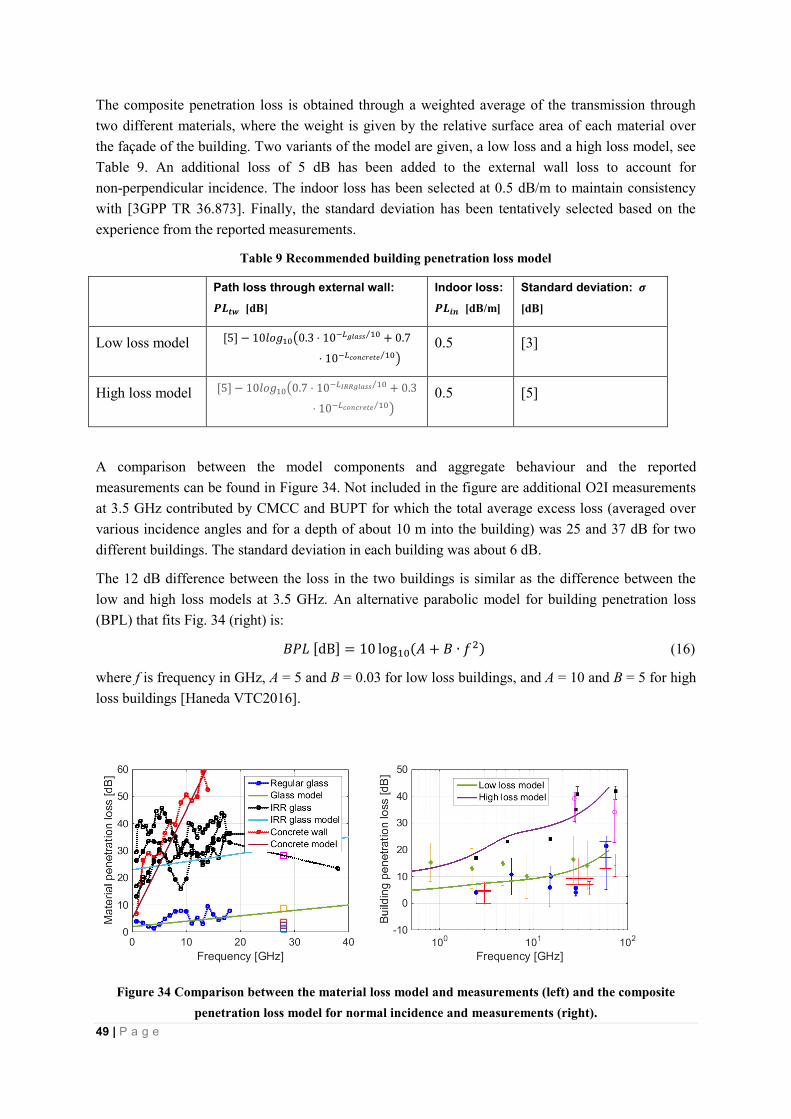
49 | P a g e
The composite penetration loss is obtained through a weighted average of the transmission through
two different materials, where the weight is given by the relative surface area of each material over
the façade of the building. Two variants of the model are given, a low loss and a high loss model, see
Table 9. An additional loss of 5 dB has been added to the external wall loss to account for
non-perpendicular incidence. The indoor loss has been selected at 0.5 dB/m to maintain consistency
with [3GPP TR 36.873]. Finally, the standard deviation has been tentatively selected based on the
experience from the reported measurements.
Table 9 Recommended building penetration loss model
Path loss through external wall:
𝑷𝑳𝒕𝒘 [dB]
Indoor loss:
𝑷𝑳𝒊𝒏 [dB/m]
Standard deviation: 𝝈
[dB]
Low loss model [5] − 10𝑙𝑜𝑔10(0.3 ⋅ 10−𝐿𝑔𝑙𝑎𝑠𝑠 10⁄ + 0.7
⋅ 10−𝐿𝑐𝑜𝑛𝑐𝑟𝑒𝑡𝑒 10⁄ ) 0.5 [3]
High loss model [5] − 10𝑙𝑜𝑔10(0.7 ⋅ 10−𝐿𝐼𝑅𝑅𝑔𝑙𝑎𝑠𝑠 10⁄ + 0.3
⋅ 10−𝐿𝑐𝑜𝑛𝑐𝑟𝑒𝑡𝑒 10⁄ ) 0.5 [5]
A comparison between the model components and aggregate behaviour and the reported
measurements can be found in Figure 34. Not included in the figure are additional O2I measurements
at 3.5 GHz contributed by CMCC and BUPT for which the total average excess loss (averaged over
various incidence angles and for a depth of about 10 m into the building) was 25 and 37 dB for two
different buildings. The standard deviation in each building was about 6 dB.
The 12 dB difference between the loss in the two buildings is similar as the difference between the
low and high loss models at 3.5 GHz. An alternative parabolic model for building penetration loss
(BPL) that fits Fig. 34 (right) is:
𝐵𝑃𝐿[dB] = 10 log10(𝐴 + 𝐵 ∙ 𝑓2) (16)
where f is frequency in GHz, A = 5 and B = 0.03 for low loss buildings, and A = 10 and B = 5 for high
loss buildings [Haneda VTC2016].
Figure 34 Comparison between the material loss model and measurements (left) and the composite
penetration loss model for normal incidence and measurements (right).

50 | P a g e
6.4 Blockage models
Dynamic blockage and geometry-induced blockage can be modelled by different modelling
approaches. The dynamic blockage could be modelled as a component of the small scale fading by
including excess shadowing on a number of paths or clusters, as has been proposed in [METIS 2015]
or [IEEE 802.11ad]. The geometry-induced blockage could be modelled as a component of the
large-scale fading as additional shadow fading with certain occurrence probability.
It is worth noting that the environment also causes transient path gains by, for example, motion of
surfaces or objects with strong reflections. The effects of transient path gains cause dynamic shadow
fading. Figure 35 illustrates the concept of static shadow fading and dynamic shadow fading. When
doing measurements in an uncontrolled environment, the measured instantaneous channel gain most
likely includes dynamic shadow fading. By taking the expectation over multiple measurements at
each Tx-Rx distance, the dynamic shadow fading can be averaged out. Path loss fitting based on the
path gain expectation values gives the static path loss and static shadow fading as described in Section
5.b .
d
PL
@t1
@tk
@t1
@tk
d
PL
Static SFDynamic blocakge
loss
Dynamic strong reflection gain
Static LS PL
Figure 35 Illustration of static shadow fading and dynamic shadow fading
7 Small Scale Fading Modelling
7.1 UMi
In the double-directional channel model, the multipath components are described by the delays and
the directions of departure and the direction of arrival. Each multipath component is scaled with a
complex amplitude gain. Then the double-directional channel impulse response is composed of the
sum of the generated double-directional multipath components. The double-directional channel model
provides a complete omni-directional statistical spatial channel model (SSCM) for both LOS and
NLOS scenarios in UMi environment. These results are analyzed based on the measurement
campaign results and mostly the ray-tracing results, which is compared with the measurement
campaign done in the same urban area.
For fast-fading modeling, ray-tracing based method is useful to extend the sparse empirical datasets
and to analyze the channel characteristics for different frequency ranges with same environments.
Ray-tracing results provide full information in spatio-temporal domain, which can be extracted to
parameterize the double-directional channel model. The large-scale parameters in SSCM are analyzed

51 | P a g e
from many measurement campaign and ray-tracing simulation, which dataset are summarized in
Appendix. As a set of example, large-scale parameters for small-scale fading model in UMi are
analyzed using the measurement campaign results and ray-tracing results on UMi street-canyon area
in Daejeon, Korea shown in Figure 36, which models the same area conducted the measurement
campaign [Hur EuCAP2015]. In the 3D ray-tracing simulation, the TX was placed 16 m above the
ground on the sixth-floor height and the RX was placed at 1.5 m above the ground. For the ray tracing
simulations, the RX was moved on a 1 m grid in a 200 m x 200 m area. The parameters for ray-tracing
simulation and environment description are similarly set to the value used in [Hur JSTSP2016].
Figure 36. Daejeon street canyon environments conducted measurement campaign and used for the
ray-tracing study. The BS location is at the sites indicated by the star and the UEs were placed outdoors
in the streets canyon areas.
The channel parameters in delay and angular domains are extracted from the detected path
information. In the SSCM approach, the channel characteristics are represented by correlated
large-scale parameters (LSPs), such as delay spread, angular spread, K-factor and shadow fading
factor, which is well described in WINNER-like channel model [WINNER]. All LSPs are modeled by
a log-normal distribution with common values of the mean μ and standard variation σ. In
[3D-SCM], the LSPs characteristics are described by these common values of log-normal
distributions, simply constant model or distance-dependent model. In this work, the new channel
model is based on the 3D-SCM approach with same assumptions, and updating the LSP parameter
tables by extending frequency up to 100 GHz. Therefore, the frequency dependency of μ and σ is
checked if the values can be modeled as a function of frequency or constant over frequency. In delay
spread, from the different dataset from measurement and ray-tracing, the linear frequency-dependency
over log10(f) is observed as shown in Figure 37. Furthermore, to avoid infinite DS values with the
frequency goes to zero, the linear regression over log10(1+f) is applied to derive the all LSP
characteristics. Also, the DS values in legacy band are close to the current channel model in 3D-SCM
parameters, which also shows the similarity of the LSP characteristics. Some parameters with weak
frequency-dependency are simply modeled as constant values by averaging the parameters over
different dataset. For further modeling purpose, other available channel parameters for extension of
LSP over frequency are described in Appendix, and those derived LPS models are summarized in
Table 10 and Table 11.

52 | P a g e
Figure 37. Delay-spread model up to 100 GHz
Table 10. Large-scale parameters for UMi Street-canyon
Scenarios UMi Street-Canyon
LOS NLOS
Delay spread (DS)
log10([s])
DS -0.2*log10(1+f) – 7.20 -0.21*log10(1+f) – 6.88
DS 0.39 0.16*log10(1+f) + 0.29
AoD spread (σASD)
log10([])
ASD -0.05*log10(1+f) + 1.21 -0.23*log10(1+f) + 1.53
ASD 0.41 0.11*log10(1+f) + 0.33
AoA spread (σASA)
log10([])
ASA -0.08*log10(1+f) + 1.73 -0.08*log10(1+f) + 1.81
ASA 0.014*log10(1+f) + 0.28 0.05*log10(1+f) + 0.3
ZoA spread (σZSA)
log10([])
ZSA -0.1*log10(1+f) + 0.73 -0.04*log10(1+f) + 0.92
ZSA -0.04*log10(1+f) + 0.34 -0.07*log10(1+f) + 0.41
Delay scaling parameter r 3 2.1
1.The trend of frequency-dependent on LSP is not observed over all measurement data
1 2 3 5 10 15 20 30 40 60 730
20
40
60
80
100
120
140
160
180
200
220
Freq [GHz]
Media
n o
f D
ela
y S
pre
ad [
ns]
LSP Analysis - RMS Delay Spread
Median DS (LoS)
Median DS (NLoS)
LinearFitted DSLoS
= -16.0 log10
(1+f) + 63.4
LinearFitted DSNLoS
= -38.0 log10
(1+f) + 126.5

53 | P a g e
Table 11. ZoD model parameters for UMi Street-canyon
Scenarios UMi Street-Canyon
LOS NLOS
ZoD spread
(σZSD)log10([])
µZSD max[-0.21, -14.8(d2D
/1000) + 0.83] max[-0.5, -3.1(d2D
/1000)+0.2]
ZSD 0.35 0.35
ZoD offset µoffset,ZOD 0 -10^{-1.5log10(max(10, d2D
))+3.3}
The channel datasets have been analyzed in the spatio-temporal domain applying Agglomerative
Algorithm [Walter 2008], for clustering such as delays, angles at the TX and RX side, and the
received powers within clusters. Based on the observed clusters in each link, large-scale parameters
such as number of clusters and intra-cluster delay spreads and angle spreads are analyzed using the
framework in [3D-SCM], and all parameters are extracted by following the methodologies in
[WINNER].
The cluster parameters are preliminary derived from some measurement and ray-tracing data, which
can be as a preliminary parameters and summarized in Appendix. The ray-tracing data predicts fewer
clusters and weak-frequency dependent characteristics. However, the clustering results based on
ray-tracing are limited due to some simulation conditions, such as small number of observed path in
simulation and the deterministic characteristic of propagation simulation. Further measurement
campaigns will be needed to verify these observations. Meanwhile, as a starting point the number of
cluster and number of rays in 3D-SCM parameters can be used. Furthermore, in some case it is also
required to modify the clustering model to support large BWs and large-sized arrays. It is
recommended to further study this through measurements with large bandwidths and/or large antenna
arrays.
Table 12. Cluster parameters for UMi Street-canyon
Scenarios 3D-UMi
LOS NLOS
Number of cluster1) 12 19
Number of rays per cluster 20 20
Cluster DS ClusterDS
-12.0*log10(1+f) + 36.6 11
Cluster ASD ClusterASD
3 10
Cluster ASA ClusterASA
17 22

54 | P a g e
Cluster ZSA ClusterZSA
7 7
Cluster SF 𝜎𝐶𝑙𝑢𝑠𝑡𝑒𝑟𝑆𝐹 5 3.09*log10(1+f) + 5.72
1. Ray-tracing results show smaller number of clusters, and recommend to study the effect of large BW and
arrays. Currently, it is suggested to use the 3GPP 3D number of clusters as a starting point.
7.2 UMa
UMa large-scale fading parameters were determined using measurements at 28 GHz in Lindholmen
and Molndal Sweden, 6 GHz data taken on the BUPT campus, and a ray-tracing study performed in
Aalborg, Denmark as shown in Figure 38. This ray tracing environment was chosen as there were
real-world measurements also made in the same area [Nguyen16]. Specifically there were two APs
used in the study which both have a height of 25 m. The UE height was 1.5 m and isotropic antennas
were employed at both the AP and UE. Note that no other objects, such as vehicles, trees, light poles,
and signs, were included in this ray-tracing study but they were present when measurements were
taken. The maximum number of rays in the simulation was 20, no transmissions through buildings
were allowed, the maximum number of reflections was four, the maximum number of diffractions
was one for frequencies above 10 GHz and was two for frequencies of 10 GHz and below. Six
frequencies were considered in this study which were 5.6, 10, 18, 28, 39.3, and 73.5 GHz.
Two philosophies were used in determining the final set of UMa parameters since there was a very
limited set of data available. The first was to make the model consistent with the 3GPP model below
6 GHz and second was to use ray tracing mostly to determine trends (e.g., how delay spread changes
with frequency) instead of absolute values of the LSPs. The large-scale parameters found for the
NLOS and LOS UMa environment are given in the Appendix (Table 23 through Table 36). The delay
and azimuth angle spreads were found to decrease in frequency and are modelled as a linear decrease
with the log of frequency. No clear frequency trend was found for the correlation of the LSPs so it
was determined to reuse the ones from the 3GPP 3D channel model. Also there was no clear
evidence to change the correlation distances of the LSPs, so again the values from the 3GPP 3D
channel model were retained.
Finally, an investigation into the clustering of the rays in this ray-tracing study was performed. To
determine clusters, the agglomerative algorithm was employed. The results showed that the average
number of clusters and the average number of rays per cluster were both fairly consistent across the
different carrier frequencies. However, the cluster delay spreads tended to decrease with increasing
frequency in both LOS and NLOS and hence it was determined to model that frequency dependency.
In interpreting these results, especially the average number of rays per cluster, it should be noted that
the number of modelled rays was limited to 20 in the simulations, Hence it was decided to still retain
the 3GPP modelling of the number of clusters and the number of rays per cluster until more study
with addition measurements or more detailed ray tracing is available.

55 | P a g e
Figure 38. Aalborg, Denmark environment used for ray-tracing study. The AP (Tx) location was at
the site indicated and UEs were placed outdoors in the streets and open areas.
7.3 InH
For InH scenarios, an investigation of small scale fading modelling has been conducted based on both
measurement and ray-tracing. Both indoor office and shopping mall environments have been
investigated at frequencies including 2.9GHz, 3.5GHz, 6GHz, 14GHz, 15GHz, 20 GHz, 28 GHz,
29GHz, 60GHz, and 73 GHz. Some preliminary analysis on large-scale channel characteristics have
been summarized from Table 37to Table 41. Some small-scale channel characteristics have been
summarized in Table 42 and Table 43. Although it is still too early to apply these results to the full
frequency range up to 100 GHz, these preliminary investigations have provided insight into the
differences across the extended frequency range.
The preliminary analysis results shown in Table 13 and Table 14 illustrate the frequency dependency
of large-scale channel characteristics across the measured frequency range. For some LSPs, frequency
dependency can be observed, but for some other LSPs, the frequency dependency observed is not
strong. Since for some cases, the number of data samples for frequencies available for analysis is
limited, it is not easy to come to conclusion yet. And also for certain measurement, frequency
dependency is not observed. These observations indicate that, for some of the LSPs, frequency
dependency could be considered for channel modelling for the frequency range up to 100 GHz.
Table 13. Analysis on frequency dependency on LSP for indoor office
Model
LOS NLOS
fitting Avg. IMT-A1 fitting Avg. IMT-A
1
DS Median [ns] -0.77*log10(1+f)+30.61 28.22 N/A -11.64*log10(1+f)+54.53 38.94 N/A
μDS -0.28*log10(1+f)-7.31 -7.71 -7.70 -0.35*log10(1+f)-7.06 -7.55 –7.41
σDS 0.04*log10(1+f)+0.18 0.24 0.18 0.10*log10(1+f)+0.04 0.19 0.14

56 | P a g e
ASA Median [°] 11.47*log10(1+f)+9.23 26.77 N/A -17.89*log10(1+f)+71.83 44.48 N/A
μASA 0.07*log10(1+f)+1.39 1.51 1.62 -0.22*log10(1+f)+1.98 1.6 1.77
σASA 1.78*log10(1+f)-2.46 0.60 0.22 1.90*log10(1+f) -2.66 0.6 0.16
ZSA Median [°] -5.90*log10(1+f)+29.77 7.13 N/A -0.56*log10(1+f)+8.14 5.97 N/A
μZSA -0.52*log10(1+f)+1.60 0.76 N/A -0.03*log10(1+f)+0.89 0.77 N/A
σZSA 0.07*log10(1+f)+0.005 0.12 N/A 0.08 0.08 N/A
K μK 0.84*log10(1+f)+2.12 3.38 7 N/A N/A N/A
σK -0.58*log10(1+f)+6.19 4.16 4 N/A N/A N/A
ASD μZSD N/A 1.08 1.60 N/A N/A 1.62
σZSD N/A 0.23 0.18 N/A N/A 0.25
ZSD μZSD N/A 0.40 N/A N/A N/A N/A
σZSD N/A 0.23 N/A N/A N/A N/A
1.The IMT-A results for InH are based on 2D channel model
Table 14. Analysis on frequency dependency on LSP for shopping mall
Model
LOS NLOS
fitting Avg. IMT-A1 fitting Avg. IMT-A
1
DS Median [ns] -13.31*log10(1+f)+60.24 41.75 N/A -23.90*log10(1+f)+89.31 56.12 N/A
μDS -0.13*log10(1+f)-7.27 -7.47 -7.70 -0.13*log10(1+f)-7.01 -7.21 –7.41
σDS 0.007*log10(1+f)+0.30 0.31 0.18 0.007*log10(1+f)+0.19 0.21 0.14
ASA Median [°] -19.01*log10(1+f)+67.41 39.06 N/A 5.43*log10(1+f)+29.02 37.13 N/A
μASA -0.21*log10(1+f)+1.83 1.51 1.62 0.10*log10(1+f)+1.54 1.7 1.77
σASA -0.08*log10(1+f)+0.38 0.25 0.22 -0.13*log10(1+f)+0.35 0.15 0.16
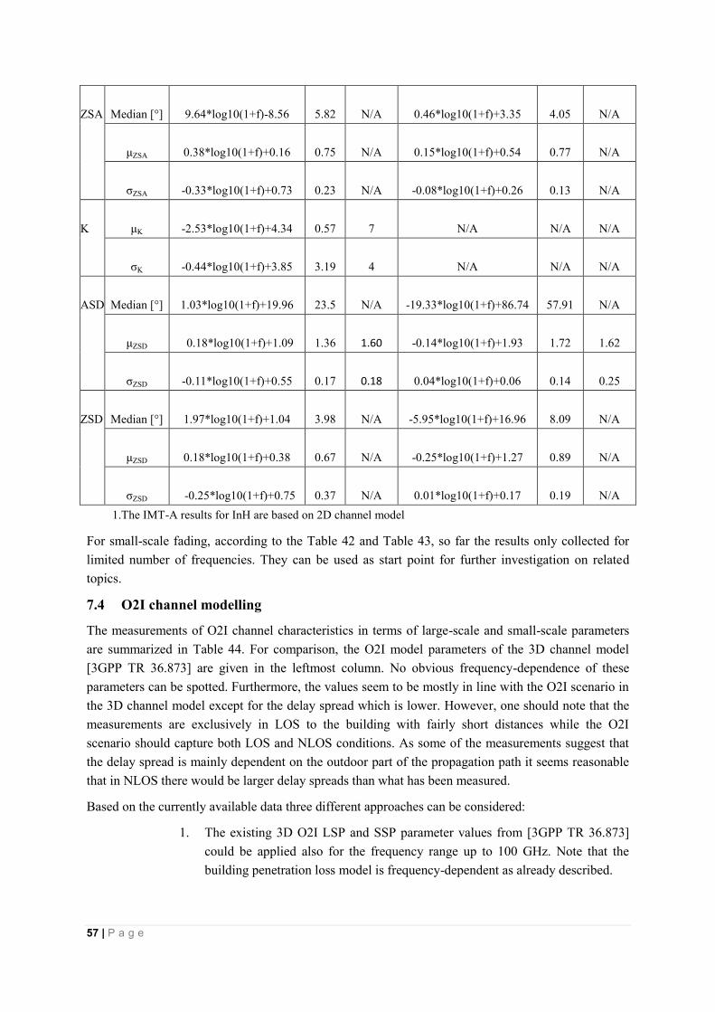
57 | P a g e
ZSA Median [°] 9.64*log10(1+f)-8.56 5.82 N/A 0.46*log10(1+f)+3.35 4.05 N/A
μZSA 0.38*log10(1+f)+0.16 0.75 N/A 0.15*log10(1+f)+0.54 0.77 N/A
σZSA -0.33*log10(1+f)+0.73 0.23 N/A -0.08*log10(1+f)+0.26 0.13 N/A
K μK -2.53*log10(1+f)+4.34 0.57 7 N/A N/A N/A
σK -0.44*log10(1+f)+3.85 3.19 4 N/A N/A N/A
ASD Median [°] 1.03*log10(1+f)+19.96 23.5 N/A -19.33*log10(1+f)+86.74 57.91 N/A
μZSD 0.18*log10(1+f)+1.09 1.36 1.60 -0.14*log10(1+f)+1.93 1.72 1.62
σZSD -0.11*log10(1+f)+0.55 0.17 0.18 0.04*log10(1+f)+0.06 0.14 0.25
ZSD Median [°] 1.97*log10(1+f)+1.04 3.98 N/A -5.95*log10(1+f)+16.96 8.09 N/A
μZSD 0.18*log10(1+f)+0.38 0.67 N/A -0.25*log10(1+f)+1.27 0.89 N/A
σZSD -0.25*log10(1+f)+0.75 0.37 N/A 0.01*log10(1+f)+0.17 0.19 N/A
1.The IMT-A results for InH are based on 2D channel model
For small-scale fading, according to the Table 42 and Table 43, so far the results only collected for
limited number of frequencies. They can be used as start point for further investigation on related
topics.
7.4 O2I channel modelling
The measurements of O2I channel characteristics in terms of large-scale and small-scale parameters
are summarized in Table 44. For comparison, the O2I model parameters of the 3D channel model
[3GPP TR 36.873] are given in the leftmost column. No obvious frequency-dependence of these
parameters can be spotted. Furthermore, the values seem to be mostly in line with the O2I scenario in
the 3D channel model except for the delay spread which is lower. However, one should note that the
measurements are exclusively in LOS to the building with fairly short distances while the O2I
scenario should capture both LOS and NLOS conditions. As some of the measurements suggest that
the delay spread is mainly dependent on the outdoor part of the propagation path it seems reasonable
that in NLOS there would be larger delay spreads than what has been measured.
Based on the currently available data three different approaches can be considered:
1. The existing 3D O2I LSP and SSP parameter values from [3GPP TR 36.873]
could be applied also for the frequency range up to 100 GHz. Note that the
building penetration loss model is frequency-dependent as already described.

58 | P a g e
2. The existing 3D O2I LSP and SSP parameter values from [3GPP TR 36.873]
could be modified to reflect the new measurements. All parameters are
modelled as frequency-independent except the building penetration loss.
3. Split the O2I scenario into a LOS variant parameterized using the new
measurements in Table 44, and a NLOS variant parameterized using possible
future NLOS O2I measurements.
8 Step-by-step procedure for generating channels
The 12-step procedure described in 36.873 should serve as a good starting point for modelling of
channels up to 100 GHz. Some modifications of existing steps or additions of new steps may be
required to comply with the modelling proposals presented in this white paper.

59 | P a g e
9 List of contributors
This paper reflects the outcome from an ad-hoc industry working group that included the following
participants.
Company Contact name Email Address
Aalto University Katsuyuki Haneda
Sinh Le Hong Nguyen
Jan Jarvelainen
Afroza Khatun
BUPT Jianhua Zhang
Lei Tian
CMCC Guangyi Liu
Hui Tong
Yi Zheng
Ericsson Henrik Asplund [email protected]
Huawei Wen Tong
Jian Li
Yi Wang
David Steer
Tommi Jamsa
Jia He
INTEL Clara Li
Tommaso Balercia
Yuan Zhu
Wenting Chang
KT Corporation Sunguk Lee
YoungSuk Kim
Nokia Amitava Ghosh
Tim Thomas
NTT DOCOMO Takehiro Nakamura
Yuichi Kakishima
Tetsuro Imai
Haralabos Papadopoulas
Koshiro Kitao
NYU Theodore (Ted) S.
Rappaport
George R. MacCartney Jr.
Mathew K. Samimi
Shu Sun
Qualcomm Ozge Koymen [email protected]
Samsung Sooyoung Hur
Jeongho Park
Charlie Zhang

60 | P a g e
Kuyeon Whang [email protected]
University of Bristol Evangelos Mellios [email protected]
University of Southern
California
Andreas F.Molisch [email protected]
10 Acknowledgements
ETRI has contributed with measurement results that have been included in the analysis and processing
performed by the contributors.
Company Contact name Email Address
ETRI Myung-Don Kim
Jae-Joon Park

61 | P a g e
11 Appendix
11.1 Overview of measurement campaigns
The basis for this white paper is the open literature in combination with recent and ongoing
propagation channel measurements performed by the cosignatories of this white paper, some of
which are as yet unpublished. These measurements along with the main observations and
conclusions are described in the accompanying Annex. The following tables give an overview of
these recent measurement activities in different frequency bands and scenarios.
11.1.1 UMi street canyon O2O
Ban
d
Party GHz Pathloss &
Shadowing Large Scale
Parameters Small Scale
Parameters
< 3
0 G
Hz
NYU 1.8 ● ● ●
CMCC/BUPT 6 ● ● Aug.
DCM 8 ●
CMCC/BUPT 10 TBD TBD
Intel 10 July. Sep. Sep.
Nokia/Aalborg 2, 10, 18 ●
CMCC 14 Sep. Sep.
Aalto 15 Sep. Sep. Sep.
Huawei 15
Ericsson 15 ● ● ●
DCM 20, 26 ● Sep. (20) Sep. (20)
Huawei 28 ● Nov. Nov.
Intel 28 Sep. Nov. Nov.
NYU 28 ● [Summer
2012]
● [Summer
2012]
● [Summer 2012]
NYU 28 Sep. Sep. Sep.
Samsung 28 ● ● ●
Ericsson 28
Nokia/Aalborg 28 ● ●
CMCC/BUPT 28 Sep. Sep.
Aalto 28 ● ● ●

62 | P a g e
Qualcomm 29 Oct. TBD TBD
Ban
d
Party GHz Pathloss &
Shadowing Large Scale
Parameters Small Scale
Parameters
30
- 6
0 G
Hz
Huawei 30-40
DCM 37 ●
NYU 38
Intel 40, 60 July (60)
Sep. (40)
Sep (60)
Nov. (40)
Sep. (60)
Nov. (40)
Ericsson 60
Huawei 60 Nov. Nov. Nov.
Qualcomm 60 Oct. TBD TBD
> 6
0 G
Hz
Aalto 63 Sep. Sep. Sep.
Huawei 73 ● Nov. Nov.
NYU 73 ● [Summer
2013 ]
● [Summer
2013 ]
● [Summer 2013
]
Intel 75, 82 Sep. Nov. Nov.
11.1.2 UMi open square O2O
Ban
d
Party GHz Pathloss &
Shadowing Large Scale
Parameters Small Scale
Parameters
< 3
0 G
Hz Nokia / AAU 10 ● Madrid-grid
CMCC/BUPT 14 Sep. Sep.
Nokia / AAU 2, 10,18 ●
Nokia/AAU 28 ●

63 | P a g e
Samsung 28 TBD
(July or Sep)
TBD (Sep) TBD (Sep)
Qualcomm 29 ● TBD TBD
30 -
60
GH
z
Qualcomm 60 Sept TBD TBD
Univ. of Bristol 60 TBD (Spring
2016)
TBD (Spring
2016)
TBD (Spring 2016)
> 6
0 G
Hz
Aalto 63 ● ● ●
NYU 73 ● [Spring
2014]
● [Spring 2014]
11.1.3 UMi O2I
Ban
d
Party GHz Pathloss &
Shadowing
Large
Scale
Parameters
Small
Scale
Parameters
< 3
0 G
Hz
NYU 1.9, 5.85 ●
DCM 8, 26 July
Nokia/Aalborg 10 ●
Ericsson 6, 15, 28 ● ● ●
Nokia/Aalborg 20 ●
Nokia/Aalborg 28 Sep.
Samsung 28 TBD (July)
NYU 28 ● [Summer
2012]
● [Summer
2012]
Ericsson 28
11.1.3.1.1.1 CMCC/BUPT 11.1.3.1.1.2 3.5 ● ●

64 | P a g e
30 -
60
GH
z
DCM 37 July
Ericsson 60 ● ● ●
> 6
0 G
Hz
11.1.4 UMa O2O
Ban
d
Party GHz Pathloss &
Shadowing Large Scale
Parameters Small Scale
Parameters
< 3
0 G
Hz
CMCC/BUPT 6 ● ● ●
Nokia/Aalborg 2, 10, 18,
28
●
CMCC/BUPT 14 TBD TBD
30 -
60
GH
z
NYU 38 ● [Summer
1998 &
Summer 2011]
● [Summer 1998
& Summer 2011]
> 6
0 G
Hz

65 | P a g e
11.1.5 InH open-plan office
Ban
d
Party GHz Pathloss &
Shadowing Large Scale
Parameters Small Scale
Parameters
< 3
0 G
Hz
NYU 1.3, 1.9,
2.5, 4.0,
5.85
● ●
CMCC/BUPT 6 Sep. Sep.
CMCC/BUPT 14 ● ●
Ericsson 15
Huawei 15 Sept. Nov. Nov.
DCM 8, 20, 26 ● Sep (20) Sep (20)
Huawei 28 ● Sept. Nov.
NYU 28 ● [Summer
2012 &
Summer 2014]
● [Summer
2012 & Summer
2014]
Samsung 28 TBD TBD TBD
Ericsson 28 TBD
CMCC 28 Sep. Sep.
30 -
60
GH
z
Huawei 30-40
DCM 37 July
Ericsson 60
NYU 60 ● [2000] ● [2000]
Univ. of Bristol 60 TBD (Spring
2016)
TBD (Spring
2016)
TBD (Spring 2016)
Huawei 60 Sept. Nov. Nov.
> 6
0
GH
z
Aalto 63, 70 ● ● ●
Huawei 72 ● Sept. Nov.

66 | P a g e
NYU 73 ● [Spring &
Summer 2014]
● [Spring &
Summer 2014]
11.1.6 InH closed-plan office
Ban
d
Party GHz Pathloss &
Shadowing Large Scale
Parameters Small Scale
Parameters
< 3
0 G
Hz
NYU 1.3, 1.9,
2.5, 4.0,
5.85
● ●
Intel 10, 28 Sep Nov Nov
Ericsson 2, 4, 6, 15 ● ● ●
NYU 28 ● [Summer
2012 &
Summer 2014]
● [Summer
2012 & Summer
2014]
Samsung 28 TBD TBD TBD
Ericsson 28 TBD
Qualcomm 29 ● TBD TBD
30 -
60
GH
z
Intel 40 Sep Nov Nov
Ericsson 60 ● ● ●
NYU 60 ● [2000] ● [2000]
Qualcomm 60 July TBD TBD
>
60
GH z
Aalto 63, 70 ● ● ●

67 | P a g e
NYU 73 ● [Spring &
Summer 2014]
● [Spring &
Summer 2014]
Intel 75, 82 Sep. Nov Nov
11.1.7 InH shopping mall
Ban
d
Party GHz Pathloss &
Shadowing Large Scale
Parameters Small Scale
Parameters
< 3
0 G
Hz
CMCC/BUPT 6 TBD TBD
Nokia/Aalborg 2, 10, 18 ●
Intel 10, 28 Sep. Nov Nov
CMCC/BUPT 14 Jul. Jul.
Aalto 15 ● ● ●
Aalto 28 ● ● ●
Samsung 28 ● ● ●
Nokia/Aalborg 28 Sep.
Qualcomm 29 June TBD
30 -
60
GH
z
Intel 40 Sep. Nov Nov
Qualcomm 60 June TBD
Univ. of Bristol 60 TBD (Spring
2016)
TBD (Spring
2016)
TBD (Spring 2016)
> 6
0 G
Hz Aalto 63, 70 ● ● ●
Intel 75, 82 Sep. Nov Nov

68 | P a g e
11.2 Overview of ray-tracing campaigns
11.2.1 UMi street canyon O2O
Ban
d
Party GHz Pathloss &
Shadowing Large Scale
Parameters Small Scale
Parameters Location Details
< 3
0 G
Hz
Aalto 15 Nov. Nov. Nov. Greater Helsinki area
Aalto 28 Nov. Nov. Nov. Greater Helsinki area
Samsung 28 ● ● ● Daejeon, Korea
/ Same location for
measurement
campaign
Samsung 28 ● ● ● Ottawa
Samsung 28 ● ● ● NYU Campus
/ Same location for
NYU measurement
campaign
USC 28 ● ● ●
Nokia 5.6,10.25,
28.5
● ● ● Madrid-grid
30 -
60
GH
z
Nokia 39.3 ● ● ● Madrid-grid
> 6
0 G
Hz
Aalto 63 Nov. Nov. Nov. Greater Helsinki area
Nokia 73 ● ● ● NYU Campus plus
Madrid-grid

69 | P a g e
11.2.2 UMi open square O2O B
an
d
Party GHz Pathloss &
Shadowing Large Scale
Parameters Small Scale
Parameters Location
Details
< 3
0 G
Hz
Nokia 5.6,10.25,
28.5
● ● ● Madrid-grid
Univ. of Bristol 28 TBD (Spring
2016)
TBD (Spring
2016)
TBD (Spring 2016) Bristol / London
30 -
60
GH
z
Nokia 39.3 ● ● ● Madrid-grid
Univ. of Bristol 40 / 60 TBD (Spring
2016)
TBD (Spring
2016)
TBD (Spring 2016) Bristol / London
> 6
0 G
Hz
Aalto 63 ● ● ● Helsinki city
center
Nokia 73.5 ● ● ● Madrid-grid
11.2.3 UMa O2O
Ban
d
Party GHz Pathloss &
Shadowing Large Scale
Parameters Small Scale
Parameters Location
Details
< 3
0 G
Hz
Nokia 5.6,10.25,
28.5
● ● ● Madrid-grid
Nokia/Aalborg 10, 18, 28 Sep. Sep. Oct. Aalborg (same
location as
measurement
campaigns)

70 | P a g e
Samsung 28 ● ● ● Ottawa
Samsung 28 ● ● ● NYU Campus
Univ. of Bristol 28 TBD (Spring
2016)
TBD (Spring
2016)
TBD (Spring 2016) Bristol / London
30 -
60
GH
z
Univ. of Bristol 40 / 60 TBD (Spring
2016)
TBD (Spring
2016)
TBD (Spring 2016) Bristol / London
Nokia/Aalborg 39.3 Sep. Sep. Oct. Aalborg (same
location as
measurement
campaigns)
Nokia 39.3 ● ● ● Madrid-grid
> 6
0 G
Hz
Nokia/Aalborg 73.5 Sep. Sep. Oct. Aalborg (same
location as
measurement
campaigns)
Nokia 73.5 ● ● ● Madrid-grid
11.2.4 InH open-plan office
Ban
d
Party GHz Pathloss &
Shadowing Large Scale
Parameters Small Scale
Parameters Location Details
< 3
0 G
Hz
Samsung 28 TBD TBD TBD (Sep) Open-Office
30 -
60
GH
z

71 | P a g e
> 6
0 G
Hz
Nokia 73 ● ● ● Open-office at
NYU campus
11.2.5 InH closed-plan office
Ban
d
Party GHz Pathloss &
Shadowing Large Scale
Parameters Small Scale
Parameters Location Details
< 3
0 G
Hz
30 -
60
GH
z
> 6
0 G
Hz
Aalto 63, 70 ● ● ● Large office,
meeting room,
cafeteria

72 | P a g e
11.2.6 InH shopping mall B
an
d
Party GHz Pathloss &
Shadowing Large Scale
Parameters Small Scale
Parameters Location Details
< 3
0 G
Hz
Samsung 28 TBD TBD TBD (Sep) Shopping-mall like
environment
/ Same location for
measurement
campaign
30 -
60
GH
z
> 6
0 G
Hz
Aalto 63, 70 ● ● ● A shopping mall in
Helsinki area

73 | P a g e
11.3 Small Scale Fading Model parameters from measurements and ray-tracing
11.3.1 UMi
Table 15. Delay spread datasets of UMi street canyon
Table 16. Angle spread ASD datasets of UMi street canyon

74 | P a g e
Table 17. Angle spread ASA datasets of UMi street-canyon
Table 18. Angle spread ZSA datasets of UMi street-canyon.
Table 19. Angle spread ZSD datasets of UMi street-canyon.

75 | P a g e
Table 20. Cluster Parameters of UMi street-canyon.
UMi Street-Canyon Ray-tracing 3GPP
3D-SCM
UMi
Samsung - Ottawa Frequency [GHz] 2.0 5.0 8.0 10.0 15.0 20.0 25.0 28.0 60.0
Number
of Cluster,
N
LoS median 6 6 6 6 6 6 5 5 5 12
NLoS median 5 6 6 5 5 5 5 5 5 19
Number of
rays per
cluster, M
LoS median 4 4 4 4 4 4 4 4 4
20 Mean 4.22 3.90 4.03 4.13 4.22 4.16 4.32 4.40 4.33
NLoS Median 2 2 2 2 3 3 3 3 3
20 Mean 4.48 4.53 4.48 4.59 4.62 4.64 4.72 4.71 4.82
Cluster DS
LoS median 31.17 25.43 24.96 24.59 23.29 21.44 21.59 17.83 13.87
NLoS median 10 13.58 13.76 13.93 11.48 10.56 10.64 11 8.04
Cluster ASD
LoS median 3.70 3.88 3.28 3.34 3.50 3.01 2.92 2.89 2.70 3
NLoS median 1.87 2.13 1.58 1.79 1.62 1.54 1.76 1.54 1.87 10
Cluster ZSA
LoS median 2.64 2.58 2.47 2.47 2.62 2.59 2.51 2.51 2.89 7
NLoS median 1.55 1.54 1.46 1.54 1.52 1.53 1.48 1.54 1.54 7
Cluster SF
LoS std 5.25 5.74 6.03 6.30 6.58 5.66 3.96 5.69 3.76 3
NLoS std 6.72 8.36 8.53 8.83 10.03 9.97 10.30 10.47 10.52 3

76 | P a g e
Figure 39. Delay Spread modeling for parameters of log-normal distributions over frequency
Figure 40. Angle Spread/ASD modeling for parameters of log-normal distributions over frequency
Figure 41. Angle Spread/ASA modeling for parameters of log-normal distributions over frequency
1 2 3 5 10 15 20 30 40 60 73 1000
0.5
1
1.5
Freq [GHz]
o
f D
ela
y S
pre
ad [
log10(s
ec)]
LSP Analysis - RMS Delay Spread
DS
(LoS)
DS
(NLoS)
LoS
= 0.39
LinearFitted NLoS
= 0.16 log10
(1+f) + 0.29
1 2 3 5 10 15 20 30 40 60 73 1000
0.2
0.4
0.6
0.8
1
Freq [GHz]
o
f A
ngle
Spre
ad-D
epart
ure
(A
SD
) [log10(d
eg)]
)
LSP Analysis - Angle Spread-Departure (ASD/Az)
ASD
(LoS)
ASD
(NLoS)
LoS
= 0.41
LinearFitted NLoS
= 0.11 log10
(1+f) + 0.33
1 2 3 5 10 15 20 30 40 60 73 1000.2
0.25
0.3
0.35
0.4
0.45
0.5
0.55
Freq [GHz]
o
f A
ngle
Spre
ad-A
rriv
al (A
SA
) [log10(d
eg)]
)
LSP Analysis - Angle Spread-Arrival (ASA/Az)
ASA
(LoS)
ASA
(NLoS)
LinearFitted LoS
= 0.014 log10
(1+f) + 0.28
LinearFitted NLoS
= 0.048 log10
(1+f) + 0.30
1 2 3 5 10 15 20 30 40 60 73 100-8
-7.8
-7.6
-7.4
-7.2
-7
-6.8
-6.6
-6.4
-6.2
Freq [GHz]
o
f D
ela
y S
pre
ad [
log10(s
ec)]
)
LSP Analysis - RMS Delay Spread
DS
(LoS)
DS
(NLoS)
LinearFitted LoS
= -0.204 log10
(1+f) + -7.20
LinearFitted NLoS
= -0.207 log10
(1+f) + -6.88
1 2 3 5 10 15 20 30 40 60 73 1000.5
1
1.5
2
Freq [GHz]
o
f A
ngle
Spre
ad-D
epart
ure
(A
SD
) [log10(d
eg)]
)
LSP Analysis - Angle Spread-Departure (ASD/Az)
ASD
(LoS)
ASD
(NLoS)
LinearFitted LoS
= -0.053 log10
(1+f) + 1.21
LinearFitted NLoS
= -0.226 log10
(1+f) + 1.53
1 2 3 5 10 15 20 30 40 60 73 1001
1.5
2
2.5
Freq [GHz]
o
f A
ngle
Spre
ad-A
rriv
al (A
SA
) [log10(d
eg)]
)
LSP Analysis - Angle Spread-Arrival (ASA/Az)
ASA
(LoS)
ASA
(NLoS)
LinearFitted LoS
= -0.080 log10
(1+f) + 1.73
LinearFitted NLoS
= -0.079 log10
(1+f) + 1.81

77 | P a g e
Figure 42. Angle Spread/ZSA modeling for parameters of log-normal distributions over frequency
Table 21. Preliminary UMi cluster parameters
28 GHz1 73 GHz2
LoS
NLoS LoS
(28-73 Combined) NLoS
Clustering Algorithm K-Means algorithm K-Means algorithm
Ave. number of clusters 6 6 5.0 4.6
Ave. number of rays per cluster 10 10 12.4 13.2
Cluster DS (nsec) TBD TBD TBD TBD
Cluster ASA (degrees) 3.3 6.7 6.7 5.2
Cluster ASD (degrees) 2.7 5.7 1.5 2.1
Cluster ZSA (degrees) 3.9 4.9 1.8 1.5
Cluster ZSD (degrees) 1.2 1.6 N/A 0.8
Per-cluster shadow fading (dB) 5 5 13.6 17.4
1 2 3 5 10 15 20 30 40 60 73 1000
0.1
0.2
0.3
0.4
0.5
0.6
0.7
0.8
0.9
1
Freq [GHz]
o
f A
ngle
Spre
ad-A
rriv
al (Z
SA
) [log10(d
eg)]
)
LSP Analysis - Angle Spread-Arrival (ZSA/Az)
ZSA
(LoS)
ZSA
(NLoS)
LinearFitted LoS
= -0.035 log10
(1+f) + 0.34
LinearFitted NLoS
= -0.071 log10
(1+f) + 0.41
1 2 3 5 10 15 20 30 40 60 73 1000.2
0.4
0.6
0.8
1
1.2
1.4
1.6
Freq [GHz]
o
f A
ngle
Spre
ad-A
rriv
al (Z
SA
) [log10(d
eg)]
)
LSP Analysis - Angle Spread-Arrival (ZSA/Az)
ZSA
(LoS)
ZSA
(NLoS)
LinearFitted LoS
= -0.096 log10
(1+f) + 0.73
LinearFitted NLoS
= -0.040 log10
(1+f) + 0.92
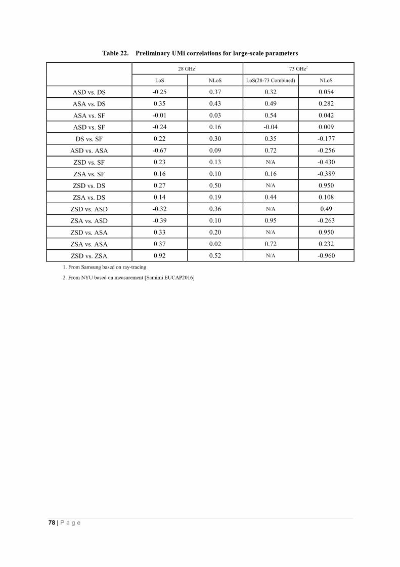
78 | P a g e
Table 22. Preliminary UMi correlations for large-scale parameters
28 GHz1 73 GHz2
LoS
NLoS LoS(28-73 Combined) NLoS
ASD vs. DS -0.25 0.37 0.32 0.054
ASA vs. DS 0.35 0.43 0.49 0.282
ASA vs. SF -0.01 0.03 0.54 0.042
ASD vs. SF -0.24 0.16 -0.04 0.009
DS vs. SF 0.22 0.30 0.35 -0.177
ASD vs. ASA -0.67 0.09 0.72 -0.256
ZSD vs. SF 0.23 0.13 N/A -0.430
ZSA vs. SF 0.16 0.10 0.16 -0.389
ZSD vs. DS 0.27 0.50 N/A 0.950
ZSA vs. DS 0.14 0.19 0.44 0.108
ZSD vs. ASD -0.32 0.36 N/A 0.49
ZSA vs. ASD -0.39 0.10 0.95 -0.263
ZSD vs. ASA 0.33 0.20 N/A 0.950
ZSA vs. ASA 0.37 0.02 0.72 0.232
ZSD vs. ZSA 0.92 0.52 N/A -0.960
1. From Samsung based on ray-tracing
2. From NYU based on measurement [Samimi EUCAP2016]

79 | P a g e
11.3.2 UMa
Table 23. UMa NLOS channel model parameters (part 1)
Table 24. UMa NLOS channel model parameters (part 2)

80 | P a g e
Table 25. UMa NLOS channel model parameters (part 3)
Table 26. UMa NLOS channel model parameters (part 4)

81 | P a g e
Table 27. UMa NLOS channel model parameters (part 5)
Table 28. UMa NLOS channel model parameters (part 6)

82 | P a g e
Table 29. UMa NLOS channel model parameters (part 7)

83 | P a g e
Table 30. UMa LOS channel model parameters (part 1)
Table 31. UMa LOS channel model parameters (part 2)

84 | P a g e
Table 32. UMa LOS channel model parameters (part 3)
Table 33. UMa LOS channel model parameters (part 4)

85 | P a g e
Table 34. UMa LOS channel model parameters (part 5)
Table 35. UMa LOS channel model parameters (part 6)

86 | P a g e
Table 36. UMa LOS channel model parameters (part 7)

87 | P a g e
11.3.3 InH
Table 37. Preliminary Indoor office large-scale channel characteristics (part 1)
3.5GHz1 6GHz1 20 GHz2 28GHz3 73GHz4 73GHz5 28GHz5
Scenarios LOS NLOS LOS NLOS LOS LOS Hybrid LOS NLOS LOS NLOS
Delay spread ()
log10
(seconds)
Median(ns) TBD TBD TBD TBD TBD TBD TBD 14.53 23.06 10.58 23.28
DS
TBD TBD TBD TBD -7.33 -7.75 -8.1 -7.85 -7.67 -7.97 -7.7
DS
TBD TBD TBD TBD 0.1 0.13 0.4 0.18 0.2 0.25 0.2
Delay distribution TBD TBD TBD TBD TBD Exponential Exponential Exponential
AoA spread (ASA
) log
10(degrees)
Median(deg) TBD TBD TBD TBD TBD TBD TBD 30.48 37.46 28.24 47.51
ASA
3GPP 3GPP 1.72 1.49 TBD 1.57 1.6 1.46 1.54 1.43 1.66
ASA
3GPP 3GPP 0.14 0.23 TBD 0.22 0.37 0.13 0.19 0.14 0.12
AoD spread (ASD
) log
10(degrees)
Median(deg) TBD TBD TBD TBD TBD TBD TBD TBD TBD TBD TBD
ASD
3GPP 3GPP 1.34 1.49 1.8 1.08 1.5 TBD TBD TBD TBD
ASD
3GPP 3GPP 0.15 0.08 0.09 0.23 0.26 TBD TBD TBD TBD
ZoA spread (ZSA
)
log10
(degrees)
Median(deg) TBD TBD TBD TBD TBD TBD TBD 4.37 5.71 9.9 6.24
ZSA
1.02 1.08 1.33 0.95 TBD 0.67 -0.025d+1.18 0.62 0.76 1 0.79
ZSA
0.41 0.36 0.07 0.28 TBD 0.17 0.30 0.14 0.08 0.05 0.08
ZoD spread (ZSD
)
log10
(degrees)
Median(deg) TBD TBD TBD TBD TBD TBD TBD TBD TBD TBD TBD
ZSD
1.22 1.26 1.25 1.48 0 0.40 -0.040d+1.45 TBD TBD TBD TBD
ZSD
0.23 0.67 0.25 0.09 0.48 0.23 0.33 TBD TBD TBD TBD
AoD and AoA distribution TBD TBD TBD TBD TBD Laplacian Uniform Wrapped Gaussian
ZoD and ZoA distribution Gaussian TBD TBD TBD Laplacian Laplacian Laplacian
Delay scaling parameter r TBD TBD TBD TBD TBD 1.95 2.4 2.03 1.35 2.23 1.78
XPR (dB)
XPR TBD TBD TBD TBD TBD TBD 15 10 6 TBD TBD
XPR
TBD TBD TBD TBD TBD TBD 2 7.5 10 TBD TBD

88 | P a g e
LOS Ricean K factor
(dB) *
K TBD TBD TBD TBD TBD TBD 8 TBD N/A TBD N/A
K TBD TBD TBD TBD TBD TBD 3 TBD N/A TBD N/A
1. From BUPT based on measurement
2. From DOCOMO based on measurement
3. From KT based on measurement
4. From Nokia/NYU based on ray-tracing
5. From Huawei based on measurement
Table 38. Preliminary Indoor office large-scale channel characteristics (part 2)
14GHz1 28GHz1 15GHz2 2.9GHz3 29GHz3 28GHz4 73GHz4
Scenarios LOS NLOS LOS NLOS LOS NLOS LOS NLOS LOS NLOS LOS NLOS LOS NLOS
Delay spread ()
log10
(seconds)
Median(ns) 27.78 36.92 29.35 43.16 22.9 42.4 24 45 25 36 TBD TBD TBD TBD
DS
-7.60 -7.47 -7.55 -7.41 -7.65 -7.43 -7.7 -7.4 -7.6 -7.5 TBD TBD TBD TBD
DS
0.27 0.22 0.15 0.17 0.2 0.17 0.29 0.14 0.37 0.18 TBD TBD TBD TBD
Delay distribution TBD TBD TBD TBD TBD TBD Exponential TBD TBD TBD TBD
XPR (dB)
XPR TBD TBD TBD TBD TBD TBD TBD TBD TBD TBD 14 10.4 22.8 15.4
XPR
TBD TBD TBD TBD TBD TBD TBD TBD TBD TBD 1.5 9.7 2.4 8
1. From CMCC&BUPT based on measurement
2. From Ericsson based on measurement
3. From Qualcomm based on measurement
4. From NYU based on measurement
Table 39. Preliminary Indoor office large-scale channel characteristics (part 3)
Parameters 3.5GHz1 20GHz2 28GHz3 73GHz4 28GHz5 73GHz5
LOS NLOS LOS LOS Hybrid LOS NLOS LOS NLOS
Correlation
distance (m)
DS [ns] TBD TBD TBD TBD 2.26 2.47 1.85 1.69
ASD [deg] TBD TBD TBD TBD 2.01 1.83 1.96 0.67

89 | P a g e
ASA [deg] TBD TBD TBD TBD 2.07 2.61 2.06 1.62
ZSD [deg] 4 4 TBD TBD 3.01 2/23 3.03 2.02
ZSA [deg] 4 4 TBD TBD 2.65 2.54 2.09 0.83
SF [dB] TBD TBD TBD TBD 1.64 1.14 0.28 2.45
K [dB] TBD TBD TBD TBD 1.62 1.13 0.28 2.41
Cross Correlation
ASD [deg] vs DS [s] 3GPP 3GPP 0.26 0.481 0.47 TBD TBD TBD TBD
ASA [deg] vs DS [s] 3GPP 3GPP TBD 0.5433 0.28 0.83 -0.03 0.69 -0.1
ASA [deg] vs SF [dB] TBD TBD TBD 0.0454 TBD 0.07 -0.55 -0.41 -0.13
ASD [deg] vs SF [dB] TBD TBD -0.68 0.3111 TBD TBD TBD TBD TBD
DS[s] vs SF[dB] TBD TBD -0.33 0.3318 TBD 0.44 0.35 -0.24 0.6
ASD [deg] vs ASA [deg] 3GPP 3GPP TBD 0.6236 0.15 TBD TBD TBD TBD
ASD [deg] vs K [dB] TBD TBD TBD TBD TBD TBD TBD TBD
ASA [deg] vs K [dB] TBD TBD TBD TBD TBD TBD TBD TBD
DS [s] vs K [dB] TBD TBD TBD TBD TBD TBD TBD TBD
SF [dB] vs K [dB] TBD TBD TBD TBD TBD TBD TBD TBD
ZSD [deg] vs SF [dB] 0.18 0 0.02 0.3749 TBD TBD TBD TBD TBD
ZSA [deg] vs SF [dB] 0.34 0 TBD 0.3313 TBD -0.52 -0.01 -0.68 -0.27
ZSD [deg] vs K [dB] 0 N/A TBD TBD TBD TBD TBD TBD
ZSA [deg] vs K [dB] 0.1 N/A TBD TBD TBD TBD TBD TBD
ZSD [deg] vs DS [s] 0 -0.27 0.24 0.1752 0.07 TBD TBD TBD TBD
ZSA [deg] vs DS [s] 0 -0.06 TBD 0.4963 -0.01 -0.2 -0.12 0.41 -0.24
ZSD [deg] vs ASD [deg] 0.65 0.35 0.1 -0.3449 0.21 TBD TBD TBD TBD
ZSA [deg] vs ASD [deg] 0 0.23 TBD 0.5116 0.1 TBD TBD TBD TBD
ZSD [deg] vs ASA [deg] 0 -0.08 TBD -0.0418 0.22 TBD TBD TBD TBD
ZSA [deg] vs ASA [deg] 0.62 0.43 TBD 0.6429 0.06 -0.03 -0.28 0.61 -0.37
ZSD [deg] vs ZSA [deg] 0.05 0.42 TBD 0.0975 0.44 TBD TBD TBD TBD

90 | P a g e
1. From BUPT based on measurement
2. From DOCOMO based on measurement
3. From KT based on measurement
4. From Nokia/NYU based on ray-tracing
5. From Huawei based on measurement
Table 40. Preliminary Indoor shopping mall large-scale channel characteristics (part 1)
15GHz1 28GHz1 63 GHz1 2.9GHz2 29GHz2 61GHz2 28GHz3 38GHz3 28GHz4 38GHz4
Scenario LOS NLOS LOS NLOS LOS NLOS LOS NLOS LOS NLOS LOS NLOS LOS NLOS LOS NLOS LOS NLOS LOS NLOS
Delay spread ()
log10
(seconds)
Median(ns) 45.88 49.69 33.91 39.65 25.68 38.4 49 80 57 71 39 58 TBD TBD TBD TBD TBD TBD TBD TBD
DS
-7.45 -7.31 -7.49 -7.45 -7.62 -7.46 -7.4 -7.1 -7.3 -7.2 -7.5 -7.3 -7.48 -7.28 -7.53 -7.24 -7.38 -6.88 -7.59 -6.9
DS
0.31 0.24 0.16 0.25 0.2 0.22 0.3 0.2 0.3 0.23 0.34 0.26 0.37 0.18 0.34 0.13 0.3 0.2 0.49 0.19
Delay distribution Exponential Exponential TBD TBD TBD TBD TBD TBD TBD TBD
AoA spread (ASA
) log
10(degrees)
Median(deg) 47.42 34.94 34.52 38.08 35.25 38.37 TBD TBD TBD TBD TBD TBD TBD TBD TBD TBD TBD TBD TBD TBD
ASA
1.62 1.54 1.52 1.56 1.5 1.56 TBD TBD TBD TBD TBD TBD 1.59 1.79 1.53 1.78 1.42 1.84 1.46 1.84
ASA
0.26 0.23 0.15 0.2 0.16 0.17 TBD TBD TBD TBD TBD TBD 0.31 0.08 0.27 0.11 0.26 0.18 0.37 0.09
AoD spread (ASD
) log
10(degrees)
Median(deg) 24.06 65.3 21.31 55.24 25.19 53.2 TBD TBD TBD TBD TBD TBD TBD TBD TBD TBD TBD TBD TBD TBD
ASD
1.32 1.77 1.35 1.71 1.43 1.68 TBD TBD TBD TBD TBD TBD TBD TBD TBD TBD TBD TBD TBD TBD
ASD
0.26 0.12 0.15 0.15 0.1 0.15 TBD TBD TBD TBD TBD TBD TBD TBD TBD TBD TBD TBD TBD TBD
ZoA spread (ZSA
)
log10
(degrees)
Median(deg) 3.69 3.92 4.43 4.04 9.34 4.2 TBD TBD TBD TBD TBD TBD TBD TBD TBD TBD TBD TBD TBD TBD
ZSA
0.63 0.62 0.64 0.62 0.86 0.63 TBD TBD TBD TBD TBD TBD 0.77 0.85 0.80 0.91 0.8 0.82 0.79 0.94
ZSA
0.52 0.25 0.44 0.29 0.4 0.24 TBD TBD TBD TBD TBD TBD 0.09 0.05 0.03 0.05 0.09 0.02 0.03 0.03

91 | P a g e
ZoD spread (ZSD
)
log10
(degrees)
Median(deg) 3.36 10.26 4.02 7.45 4.56 6.56 TBD TBD TBD TBD TBD TBD TBD TBD TBD TBD TBD TBD TBD TBD
ZSD
0.63 0.98 0.64 0.87 0.74 0.82 TBD TBD TBD TBD TBD TBD TBD TBD TBD TBD TBD TBD TBD TBD
ZSD
0.46 0.19 0.35 0.2 0.3 0.2 TBD TBD TBD TBD TBD TBD TBD TBD TBD TBD TBD TBD TBD TBD
AoD and AoA distribution Wrapped Gaussian TBD TBD TBD TBD TBD TBD TBD TBD TBD TBD TBD TBD TBD TBD
ZoD and ZoA distribution Laplacian TBD TBD TBD TBD TBD TBD TBD TBD TBD TBD TBD TBD TBD TBD
Delay scaling parameter r 6.79 7.17 10.23 8.62 8.7 8.31 TBD TBD TBD TBD TBD TBD TBD TBD TBD TBD TBD TBD TBD TBD
XPR (dB)
XPR 17.12 17.71 16.12 14.48 16.85 16.06 TBD TBD TBD TBD TBD TBD TBD TBD TBD TBD TBD TBD TBD TBD
XPR
5.85 6.74 6.22 6.25 6.62 5.34 TBD TBD TBD TBD TBD TBD TBD TBD TBD TBD TBD TBD TBD TBD
LOS Ricean K
factor (dB) *
K 1.36 N/A 0.54 N/A -0.18 N/A TBD N/A TBD N/A TBD N/A TBD N/A TBD N/A TBD N/A TBD N/A
K 3.49 N/A 2.91 N/A 3.18 N/A TBD N/A TBD N/A TBD N/A TBD N/A TBD N/A TBD N/A TBD N/A
1. From Aalto University based on measurement
2. From Qualcomm based on measurement
3. From ETRI based on measurement in Railway station
4. From ETRI based on measurement in Airport
Table 41. Preliminary Indoor shopping mall large-scale channel characteristics (part 2)
Parameters 15GHz1 28GHz1 63GHz1
LOS NLOS LOS NLOS LOS NLOS
Correlation
distance (m)
DS [ns] 8 2.5 8.5 2 8 0.5
ASD [deg] 7 6.5 5.5 1 2 1
ASA [deg] 17.5 7.5 6.5 6 8.5 4.5
ZSD [deg] 8.5 4.5 7.5 1.5 7.5 0.5
ZSA [deg] 12.5 3 10 1.5 14.5 2
SF [dB] 3 7.5 6.5 7.5 15 2
K [dB] 2 N/A 12.5 N/A 16 N/A

92 | P a g e
Cross Correlation
ASD [deg] vs DS [s] 0.44 0.16 -0.16 0.32 -0.1 0.54
ASA [deg] vs DS [s] 0.31 0.51 0.46 0.36 0.62 0.21
ASA [deg] vs SF [dB] -0.09 0.08 0.13 0.44 0.31 0.27
ASD [deg] vs SF [dB] 0.29 0.16 0.38 0.33 0.3 0.33
DS[s] vs SF[dB] 0.13 0.11 -0.03 0.42 0.21 0.48
ASD [deg] vs ASA [deg] -0.37 0.46 -0.3 0.35 -0.07 0.24
ASD [deg] vs K [dB] -0.18 N/A 0.34 N/A 0.41 N/A
ASA [deg] vs K [dB] -0.13 N/A -0.28 N/A -0.07 N/A
DS [s] vs K [dB] -0.49 N/A -0.46 N/A -0.38 N/A
SF [dB] vs K [dB] 0.4 N/A 0.49 N/A 0.49 N/A
ZSD [deg] vs SF [dB] -0.08 0.01 -0.14 0.29 -0.17 0.45
ZSA [deg] vs SF [dB] -0.15 0.09 -0.17 0.29 -0.19 0.23
ZSD [deg] vs K [dB] 0.01 N/A 0.37 N/A 0.56 N/A
ZSA [deg] vs K [dB] -0.07 N/A 0.38 N/A 0.45 N/A
ZSD [deg] vs DS [s] -0.43 -0.22 -0.6 0.04 -0.58 0.37
ZSA [deg] vs DS [s] -0.35 0.3 -0.5 0.36 -0.16 0.2
ZSD [deg] vs ASD [deg] 0.28 -0.08 0.21 0.4 0.46 0.33
ZSA [deg] vs ASD [deg] 0.3 -0.2 0.27 0.03 0.34 -0.1
ZSD [deg] vs ASA [deg] -0.54 -0.5 -0.45 -0.01 -0.26 -0.2
ZSA [deg] vs ASA [deg] -0.58 0.19 -0.42 0.47 0.08 0.26
ZSD [deg] vs ZSA [deg] 0.92 0.09 0.9 0.22 0.77 0.29
1. From Aalto University based on measurement

93 | P a g e
Table 42. Preliminary Indoor office small-scale channel characteristics
Parameters 73GHz1 28GHz2 28GHz3 73GHz3
Hybrid LOS LOS NLOS LOS NLOS
Number of clusters 6 7 3.271 3.5 3.9 4.3
Number of rays per cluster 10 4 52.9 41.82 38.47 35.75
Cluster ASD [deg] 3.2 9.75 TBD TBD TBD TBD
Cluster ASA[deg] 3.7 13.22 15.27 15.35 14.05 10.44
Cluster ZSD[deg] 10^(-0.043d+0.09) 3.61 TBD TBD TBD TBD
Cluster ZSA[deg] 10^(-0.036d-0.18) 5.16 8.06 5.42 3.95 4.51
Per cluster shadowing std
[dB] 12 TBD TBD TBD TBD TBD
1. From Nokia/NYU based on ray-tracing
2. From KT based on measurement
3. From Huawei based on measurement
Table 43. Preliminary Indoor shopping mall small-scale channel characteristics
Parameters 15GHz1 28GHz1 63GHz1
LOS NLOS LOS NLOS LOS NLOS
Number of clusters 6.33 6.98 6.18 6.21 6.23 5.68
Number of rays per cluster 2.7 7.9 3.67 10 7.8 14
Cluster ASD [deg] 5.2 9.87 6.59 11.12 9.98 12.82
Cluster ASA[deg] 5.22 9.34 6.73 10.05 12.27 11.4
Cluster ZSD[deg] 2.52 4.35 2.96 4.75 5.06 4.7
Cluster ZSA[deg] 2.43 2.3 3.17 2.44 6.08 3.03
Per cluster shadowing std [dB] 14 10 16 11 11 11
1. From Aalto based on measurement

94 | P a g e
11.3.4 O2I
Table 44 Summary of measured small scale channel parameters for the O2I scenario

95 | P a g e

96 | P a g e

97 | P a g e
11.4 Processing Methodologies
11.4.1 Physical effects on propagation
As a consequence of shorter wavelengths as the carrier frequency increases, the radio propagation
must be modelled with an understanding and consideration of a number of physical effects that occur
in the real environment. A deployment scenario, perhaps involving up to a hundred meters of
propagation transmission distance with short wavelengths, will encounter multiple different physical
transmission effects. It is helpful if these physical effects are included in the overall transmission
model to accurately reflect the behavior of the radio propagation environmental conditions.
An illustration of some of the physical effects of propagation is shown in Figure 43. This illustration
may be helpful in understanding the multiple regions of physical processes that may be in the
environment and affect the radio propagation.
Zone1 (close range free space)
Propagation is dominated by the direct path with few reflections.
Zone 2 (LOS/scattered/waveguide)
Propagation is dominated by the direct path and significant close reflections.
Zone 3 (NLOS occultation scattered)
Propagation is mainly by the reflections with some direct path energy but these are attenuated
by distance.
Zone 4 (distant NLOS)
Propagation is dominated by a small number of paths that are either not occulted or are a result
of a good reflection.
Zone 5 (too distant)
The illustration also shows a fifth zone in which the signals have become too weak to be useful
either through numerous multiple reflections, distance, corners or occultation. In this zone
communications is generally impractical.
Figure 43. Illustration of multiple physical transmission effects

98 | P a g e
In each region there is always the possibility of physical blockage or occultation. Because of the small
wavelengths, many typical objects in the environment (e.g. people, furniture, machinery, office
equipment, etc.) are of a size that they completely block the direct signal, leaving the receiver with
little except whatever reflections that may be available. This is shown in the illustration as typically
in Zone 3 or 4 but it may occur anywhere. Also in some instances, there may be penetration loss for
signals into interior rooms or through walls. The zone size depends on the wavelength, the
dimensions and details of the environment, and the antenna beam widths. Not all zones may exist in
every deployment environment or signal path. Typically, the signal propagation may experience
multiple physical effects on its journey and so the “zones” may overlap in space.
11.4.2 The effects of the antenna pattern
In understanding the measurements of the new 5G channels and the associated channel model
parameters, it is helpful to know the characteristics of the antennas used to make the measurements.
Some measurement antennas are directive (e.g. horn or array antennas) and consequently may not
illuminate reflecting surfaces of the environment during measurements and thus may appear to
simplify the environment when compared with measurements made with other non-directional
antennas (e.g. omni-directional antennas). In some cases, the test antennas may have significant
sidelobes in their radiation pattern and these may make the environment seem more reflective than is
physically the case.
Traditionally, measurements in the frequency bands below 6 GHz have used omni-directional
antennas. In these bands the transmit antenna “floods” the environment with power in all directions
(i.e. sector coverage) and the receive antenna accepts power from all directions at its location. In
environments in which there are many reflections the apparent “path loss” may be reduced due to the
additional power received from the many reflections. Typically in low frequency bands, the same
antenna format (i.e. sector at base station and omni-directional at user equipment) is also used for the
operational equipment and so the total-power/omni-directional path loss measurement is appropriate
for the operating environment. Propagation studies and operation for these bands has thus been
successful because the measurements, modelling and operation are all based on similar antenna
characteristics.
In the bands above 6 GHz however, directional antennas (e.g. “horns”) are often used for
measurements to help improve the range of the measurements. Directional antenna configurations
are also expected to be used for operational equipment including mobile devices and access points as
the antenna “gain” they provide may be necessary in the operational system to achieve the needed link
budget. However, if the antenna configuration used for the path loss measurements is not the same
as used for the operating equipment, then the associated model may not be accurate for modelling link
budgets for equipment having different antenna configurations. Equipment with a narrow beam
antenna will typically see less received power than would be expected based on a path loss model
derived from measurements using omni-directional antennas.
a. Decoupling the antenna pattern
Many of the future systems will be operated using highly directional antennas for at least a portion of
their usage. To accurately model these conditions it is necessary to decouple the channel model
from the measurement antenna patterns. This is often referred to as “antenna decoupling”. The
measurements are in reality the convolution of the measurement antenna patterns and the channel

99 | P a g e
environment and recovering the channel environment from the measurements involves a
“deconvolution” of the measuring antenna patterns from the measurements. The general process for
decoupling of the antenna pattern to reconstruct the true signal angular distribution can be
summarized in the following steps.
1. Estimate the path of propagation (angular domain/delay domain/both).
2. Remove the antenna pattern (different algorithms).
3. Reconstruct the estimated measured data with antenna pattern.
4. Evaluate the effect of reconstruction and antenna decoupling.
For a typical measurement antenna with a main beam and small side-lobes, the measured angular
spectrum will appear as the actual channel “blurred” by the measurement antenna sampling pattern.
To recover the true angular distribution of the actual channel it is necessary to undo the convolution
between the measuring antenna and the channel. This is not an easy to do as practical signals and
beam patterns include zeros or low amplitude regions that may prevent a simple analytical inversion
from recovering the real channel. However, with sufficiently well behaved signals (i.e. with
well-defined angular clusters and a good ratio between beam strength and its side-lobes) often a good
approximations can be made.
Similar measurement decoupling problems are experienced in a number of other sciences and there
are several algorithms for deriving the hypothetical true angular distribution from the data. Some of
these processes are iterative, in which an initial estimate is gradually corrected based on its
comparison to the measured data. A popular practical technique in the RADAR community is the
“MUSIC” algorithm [Schmidt] while the Synthetic Aperture Imaging and radio astronomy
communities use the “CLEAN” algorithm [Clarke]. The SAGE algorithm has also been applied in
this context [Fessler].
11.4.3 Clustering
Different clustering algorithms were considered in support of the channel modelling activities herein
described. These algorithms include the Agglomerative algorithm, the k-means algorithm and the time
cluster and spatial lobe clustering algorithm.
The agglomerative algorithm is a bottom-up hierarchical clustering algorithm where multipath
components (MPCs) are iteratively merged together. It starts with each MPC belonging to a different
cluster and, at each step, the most similar clusters are combined. The process repeats until either a
stop criterion is met or only one single cluster remains.
The K-means algorithm [Czink VTCF06] groups the multipath components (MPCs) into clusters
such that the MPCs within each cluster have similar delay, elevation and azimuth angles. The
algorithm identifies each cluster by its centroid position in the parameter space. Each MPC is assigned
to the cluster centroid with smallest distance. The algorithm iteratively optimizes the positions of the
centroids in order to minimize the total distance from each MPC to its centroid.
In the time cluster and spatial lobe clustering algorithm approach [Samimi GCW2015][Samimi
ICC2015] [Samimi EUCAP2016] [Samimi VTC2013] [Samimi MTT2016], the time and space
dimensions are considered independently, by separately performing data clustering in the temporal
and spatial domains, yielding statistics for time clusters and spatial lobes in omnidirectional
millimeter wave channels. Time clusters are composed of multipath components traveling close in

100 | P a g e
time delay, and that arrive from potentially different angular directions in a short propagation time
window as seen from field measurements. Spatial lobes represent main directions of arrival (or
departure) where energy arrives over the entire time span of the multipath time delay profile. In this
modelling framework, a channel impulse response “initial condition” for a particular location or point
is generated by separately generating time cluster parameters and spatial lobe parameters
independently, and then randomly assigning the different multipath components to different spatial
lobes as has been found to occur in millimeter wave channels.

101 | P a g e
References
[3GPP TR25.996] 3GPP TR 25.996 (V.12.0.0), “Spatial channel model for Multiple Input Multiple
Output (MIMO) simulations,” Sep. 2014.
[3GPP TR36.814] 3GPP TR 36.814 (V9.0.0), “Further advancements for E-UTRA physical layer
aspects ,” Mar. 2010.
[3GPP TR36.873] 3GPP, TR 36.873 (V12.2.0), “Study on 3D channel model for LTE,” July 2015
[3GPP TR38.900] 3GPP TR 38.900 (V14.0.0), “Channel model for frequency spectrum above 6
GHz”, July 2016.
[Andersen 1995] J. Andersen, T. Rappaport, and S. Yoshida, “Propagation measurements and models
for wireless communications channels,” IEEE Communications Magazine, vol. 33, no. 1, pp. 42–49,
Jan 1995.
[And2002] C. Anderson, et al., “In-Building Wideband Multipath Characteristics at 2.5 & 60 GHz,”
2002 IEEE 56th Vehicular Technology Conference (VTC2002-Fall), pp. 97-101.
[Anite Telecoms 2014] Anite Telecoms, “Some investigations on angular sampling method for 3D
spatial cluster”, 3GPP R1-140805, Prague, Czech Republic, 10 – 14 February 2014.
[Asplund et al. 2006] Asplund, Henrik, et al. "The COST 259 directional channel model-part II:
macrocells." IEEE Transactions on Wireless Communications 5.12 (2006): 3434-3450.
[Baum2015] D. S. Baum, J. Hansen, and J. Salo, “An interim channel model for beyond-3G systems:
extending the 3GPP spatial channel model (SCM),” in Proc. 2005 IEEE 61st Vehicular Technology
Conference (VTC2005-Spring), vol. 5, pp. 3132-3136.
[Chavero 1999] M. Chavero, et al., "Impact of Vegetation on the performance of 28 GHz LMDS
Transmission," IEEE MTT-S, Vol. 3, June 1999, p. 1063-1066.
[Chen 2016] X. Chen, L. Tian, P. Tang and J. H. Zhang, "Modelling of Human Body Shadowing
Based on 28 GHz Measurement Results," in Proc. 84th Veh. Tech. Conf (VTC2016-Fall), Montreal,
Canada, Sep, 2016.
[Clark Sept. 1980] An efficient implementation of the algorithm 'CLEAN'; Clark, B. G.; Astronomy
and Astrophysics, vol. 89, no. 3, pp377-378; Sept 1980.[COST] http://www.cost2100.org/
[Czink VTCF06] N. Czink, et al., “A framework for automatic clustering of parametric MIMO
channel data including path powers,” in IEEE VTC-Fall 2006, September 2006.
[ETSI 2015] ETSI, “New ETSI Group on Millimetre Wave Transmission starts work,”
http://www.etsi.org/news-events/news/866-2015-01-press-new-etsi-group-on-millimetre-wave-transm
ission-starts-work
[Fessler VTC Fall 2014] Space-Alternating Generalized Expectation-Maximization Algorithm;
Fessler, J.A.; IEEE Transactions on Signal Processing, vol. 42, no. 10, pp2664-2677; Oct 1994.
[Forkel et al. 2004] Forkel, Ingo, Marc Schinnenburg, and Markus Ang. "Generation of

102 | P a g e
two-dimensional correlated shadowing for mobile radio network simulation."WPMC, sep 21 (2004):
43.
[Gao et al. 2015] X. Gao, O. Edfors, F. Tufvesson and E. G. Larsson, "Massive MIMO in Real
Propagation Environments: Do All Antennas Contribute Equally?," in IEEE Transactions on
Communications, vol. 63, no. 11, pp. 3917-3928, Nov. 2015.
[Gao 2016] X. Gao, L. Tian, P. Tang, T. Jiang, B. Liu, J. H. Zhang "Channel Characteristics Analysis
of Angle and Clustering in Indoor Office Environment at 28 GHz," in Proc. 84th Veh. Tech. Conf
(VTC2016-Fall), Montreal, Canada, Sep, 2016.
[Gustafson 2014] C. Gustafson, et al. , “On mm-Wave Multipath Clustering and Channel Modeling,”
IEEE Transactions on Antennas and Propagation, vol. 62, no. 3, pp. 1445-1455, Mar. 2014.
[Haneda 2016] K. Haneda, N. Omaki, T. Imai, L. Raschkowski, M. Peter and A. Roivainen,
"Frequency-Agile Pathloss Models for Urban Street Canyons," in IEEE Transactions on Antennas
and Propagation, vol. 64, no. 5, pp. 1941-1951, May 2016.
[Haneda ICC2016] K. Haneda et al., “Indoor 5G 3GPP-like channel models for office and shopping
mall environments,” 2016 IEEE International Conference on Communications Workshops (ICC),
Kuala Lumpur, 2016, pp. 694-699.
[Haneda VTC2016] K. Haneda et al., "5G 3GPP-Like Channel Models for Outdoor Urban
Microcellular and Macrocellular Environments," 2016 IEEE 83rd Vehicular Technology Conference
(VTC2016-Spring), Nanjing, 2016, pp. 1-7.
[Hata 1980] M. Hata, “Empirical formulas for propagation loss in land mobile radio service,” IEEE
Trans. Veh. Technol., vol. 29, no. 3, pp. 317–325, Aug.1980
[Huang 2016] F.S.Huang, L. Tian, Y. Zheng, J. H. Zhang,"Propagation Characteristics of Indoor
Radio Channel from 3.5 GHz to 28 GHz," in Proc. 84th Veh. Tech. Conf (VTC2016-Fall), Montreal,
Canada, Sep, 2016.
[Hur EuCAP2015] S. Hur et al., "Wideband spatial channel model in an urban cellular environments
at 28 GHz," 2015 9th European Conference on Antennas and Propagation (EuCAP), Lisbon, 2015,
pp. 1-5.
[Hur JSTSP2016] S. Hur, et al., “Proposal on Millimeter-Wave Channel Modeling for 5G Cellular
System”, IEEE Journal of Selected Topics in Signal Processing, April 2016.
[ITU M.2135-1] ITU-R Rep M.2135-1, ”Guidelines for evaluation of radio interface technologies for
IMT-Advanced.”
[ITU-R P.676] Recommendation ITU-R P.676-10 “Attenuation by atmospheric gases”
[ITU-R P.833] Recommendation ITU-R P.833-8 “Attenuation in vegetation”
[ITU-R P.838] Recommendation ITU-R P.838-3 “Specific attenuation model for rain for use in
prediction methods”
[Jarvelainen 2016] J. Järveläinen, S. L. H. Nguyen, K. Haneda, R. Naderpour and U. T. Virk,
"Evaluation of Millimeter-Wave Line-of-Sight Probability With Point Cloud Data," in IEEE Wireless
Communications Letters, vol. 5, no. 3, pp. 228-231, June 2016.

103 | P a g e
[Karttunen EuCAP2015] A. Karttunen, K. Haneda, J. Jarvelainen and J. Putkonen, “Polarisation
Characteristics of Propagation Paths in Indoor 70 GHz Channels,” in Proc. 9th
European Conf. Ant.
Prop. (EuCAP 2015), Lisbon, Portugal, Apr. 2015.
[Larsson EuCAP 2014] C. Larsson, F. Harrysson, B. E. Olsson and J. E. Berg, "An outdoor-to-indoor
propagation scenario at 28 GHz," The 8th European Conference on Antennas and Propagation
(EuCAP 2014), The Hague, 2014, pp. 3301-3304.
[Lei 2014] M. Y. Lei, J. H. Zhang, L. Tian, D. T. Du, "28-GHz indoor channel measurements and
analysis of propagation characteristics." In Proc. 25th International Symposium on Personal, Indoor,
and Mobile Radio Communications (PIMRC2014), Washington DC, USA, Sep, 2014.
[Liu2012] L. Liu, C. Oestges, J. Poutanen, K. Haneda, P. Vainikainen, F. Quitin, F. Tufvesson, P. D.
Doncker, “The COST 2100 MIMO channel model,”, IEEE Wireless Communications Magazine, Dec.,
2012, pp. 92-99.
[MacCartney GC2013] G. R. MacCartney, Jr., J. Zhang, S. Nie, and T. S. Rappaport, “Path loss
models for 5G millimeter wave propagation channels in urban microcells,” in 2013 IEEE Global
Communications Conference (GLOBECOM), Dec. 2013, pp. 3948–3953.
[MacCartney 2015] G. R. MacCartney, Jr., et al, “Indoor Office Wideband Millimeter-Wave
Propagation Measurements and Channel Models at 28 GHz and 73 GHz for Ultra-Dense 5G Wireless
Networks (Invited),” IEEE Access, vol. 3, pp. 2388-2424, Oct. 2015.
[MacCartney 2016] G. R. MacCartney, Jr., S. Deng, S. Sun, and T. S. Rappaport, “Millimeter-Wave
Human Blockage at 73 GHz with a Simple Double Knife-Edge Diffraction Model and Extension for
Directional Antennas,” 2016 IEEE 84th Vehicular Technology Conference (VTC2016-Fall), Sept.
2016.
[METIS 2013] “Simulation Guidelines,” Deliverable D6.1, METIS document number
ICT-317669-METIS/D6.1, October 31, 2013.
[METIS 2015] METIS2020, Deliverable D1.4 v3, “METIS Channel Model,” July 2015.
https://www.metis2020.com/wp-content/uploads/METIS_D1.4_v3.pdf
[Miao 2015] R. Q. Miao, L. Tian, Y. Zheng, P. Tang, F.S. Huang, J.H. Zhang, "Indoor office
channel measurements and analysis of propagation characteristics at 14 GHz." In Proc. 26th
International Symposium on Personal, Indoor, and Mobile Radio Communications (PIMRC2015),
HoKong, China, Aug, 2015.
[MiWEBA 2014] MiWEBA, Deliverable D5.1 “Channel modeling and characterization,” June,
2014, http://www.miweba.eu/wp-content/uploads/2014/07/MiWEBA_D5.1_v1.011.pdf.
[mmMagic] https://5g-ppp.eu/mmmagic/
[Molisch et al. 2006] Molisch, Andreas F., et al. "The COST259 directional channel model-part I:
Overview and methodology." IEEE Transactions on Wireless Communications 5.12 (2006):
3421-3433.
[Molisch et al. 2016] A. F. Molisch, A. Karttunen, S. Hur, J. Park and J. Zhang, "Spatially consistent
pathloss modeling for millimeter-wave channels in urban environments," 2016 10th European

104 | P a g e
Conference on Antennas and Propagation (EuCAP), Davos, 2016
[Nie13] S. Nie, G. R. MacCartney, Jr., S. Sun, T. S. Rappaport, “72 GHz Millimeter Wave Indoor
Measurements for Wireless and Backhaul Communications,” in 2013 IEEE 24th Annual International
Symposium on Personal, Indoor and Mobile Radio Communications, (PIMRC), Sept. 2013, pp. 2429.
[NIST] http://www.nist.gov/ctl/wireless-networks/5gmillimeterwavechannelmodel.cfm
[Nguyen16] H. C. Nguyen, et al., “An Empirical Study of Urban Macro Propagation at 10, 18 and 28
GHz,” 2016 IEEE 83rd Vehicular Technology Conference (VTC2016-Spring), Nanjing, 2016, pp. 1-5.
[Ökvist 2016] P. Ökvist, N. Seifi, B. Halvarsson, A. Simonsson, M. Thurfjell, H. Asplund and J.
Medbo, “15 GHz Street-Level Blocking Characteristics Assessed with 5G Radio Access Prototype,”
2016 IEEE 83rd Vehicular Technology Conference (VTC2016-Spring), Nanjing, 2016, pp. 1-5.
[Piersanti ICC2012] S. Piersanti, L. Annoni, and D. Cassioli, “Millimeter waves channel
measurements and path loss models,” in 2012 IEEE International Conference on Communications
(ICC), June 2012, pp. 4552–4556.
[R1-160846] 3GPP R1-160846, Ericsson, “Street Microcell Channel Measurements at 2.44, 14.8 &
58.68 GHz”, Feb. 2016. Online:
ftp://ftp.3gpp.org/TSG_RAN/WG1_RL1/TSGR1_84/Docs/R1-160846.zip
[Rappaport 2013] T. S. Rappaport et al., "Millimeter Wave Mobile Communications for 5G Cellular:
It Will Work!," in IEEE Access, vol.1, pp. 335-349, 2013.
[Rappaport 2015], T. S. Rappaport, G. R. MacCartney, M. K. Samimi and S. Sun, "Wideband
Millimeter-Wave Propagation Measurements and Channel Models for Future Wireless
Communication System Design," in IEEE Transactions on Communications, vol. 63, no. 9, pp.
3029-3056, Sept. 2015.
[Rappaport Book2015] T. S. Rappaport, R. W. Heath, Jr., R. C. Daniels, and J. N. Murdock,
Millimeter Wave Wireless Communications. Pearson/Prentice Hall 2015.
[Rappaport ICC 2015] T. S. Rappaport and S. Deng, "73 GHz wideband millimeter-wave foliage and
ground reflection measurements and models," 2015 IEEE International Conference on
Communication Workshop (ICCW), London, 2015, pp. 1238-1243.
[Rodriguez VTC Fall 2014] I. Rodriguez, H. C. Nguyen, N. T. K. Jorgensen, T. B. Sorensen and P.
Mogensen, "Radio Propagation into Modern Buildings: Attenuation Measurements in the Range from
800 MHz to 18 GHz," 2014 IEEE 80th Vehicular Technology Conference (VTC2014-Fall),
Vancouver, BC, 2014, pp. 1-5.
[Samimi VTC2013] M. K. Samimi et al., "28 GHz Angle of Arrival and Angle of Departure Analysis
for Outdoor Cellular Communications Using Steerable Beam Antennas in New York City," 2013
IEEE 77th Vehicular Technology Conference (VTC2016-Spring), Dresden, 2013, pp. 1-6.
[Samimi 2015] M. K. Samimi, T. S. Rappaport, and G. R. MacCartney, Jr., “Probabilistic
omnidirectional path loss models for millimeter-wave outdoor communications,” in IEEE Wireless
Communications Letters, vol. 4, no. 4, pp. 357-360, Aug. 2015.

105 | P a g e
[Samimi GCW2015] M. K. Samimi and T. S. Rappaport, "Statistical Channel Model with
Multi-Frequency and Arbitrary Antenna Beamwidth for Millimeter-Wave Outdoor Communications,"
2015 IEEE Globecom Workshops (GC Wkshps), San Diego, CA, 2015, pp. 1-7.
[Samimi ICC2015] M. K. Samimi and T. S. Rappaport, "3-D statistical channel model for
millimeter-wave outdoor mobile broadband communications," 2015 IEEE International Conference
on Communications (ICC), London, 2015, pp. 2430-2436.
[Samimi GC2014] M. K. Samimi and T. S. Rappaport, "Ultra-wideband statistical channel model for
non line of sight millimeter-wave urban channels," 2014 IEEE Global Communications Conference,
Austin, TX, 2014, pp. 3483-3489.
[Samimi EUCAP2016] M. K. Samimi and T. S. Rappaport, "Local multipath model parameters for
generating 5G millimeter-wave 3GPP-like channel impulse response," 2016 10th European
Conference on Antennas and Propagation (EuCAP), Davos, 2016, pp. 1-5.
[Samimi MTT2016] M. K. Samimi and T. S. Rappaport, "3-D Millimeter-Wave Statistical Channel
Model for 5G Wireless System Design," in IEEE Transactions on Microwave Theory and Techniques,
vol. 64, no. 7, pp. 2207-2225, July 2016.
[Schwering 1988] F. Schwering, et al., "Millimeter-Wave Propagation in Vegetation: Experiments
and Theory," IEEE Trans. Geoscience and Remote Sensing, vol. 23, no. 6, p.355-367, May 1988.
[Schmidt Mar 1986] R. Schmidt, "Multiple emitter location and signal parameter estimation," in IEEE
Transactions on Antennas and Propagation, vol. 34, no. 3, pp. 276-280, Mar 1986.
[Semaan Globecom 2014] E. Semaan, F. Harrysson, A. Furuskär and H. Asplund, "Outdoor-to-indoor
coverage in high frequency bands," 2014 IEEE Globecom Workshops (GC Wkshps), Austin, TX, 2014,
pp. 393-398.
[Sun GCW2015] S. Sun, T. A. Thomas, T. S. Rappaport, H. Nguyen, I. Z. Kovacs and I. Rodriguez,
"Path Loss, Shadow Fading, and Line-of-Sight Probability Models for 5G Urban Macro-Cellular
Scenarios," 2015 IEEE Globecom Workshops (GC Wkshps), San Diego, CA, 2015, pp. 1-7.
[Sun VTCS2016] S. Sun et al., "Propagation Path Loss Models for 5G Urban Micro- and
Macro-Cellular Scenarios," 2016 IEEE 83rd Vehicular Technology Conference (VTC2016-Spring),
Nanjing, 2016, pp. 1-6.
[Sun TVT2016] S. Sun et al., "Investigation of Prediction Accuracy, Sensitivity, and Parameter
Stability of Large-Scale Propagation Path Loss Models for 5G Wireless Communications," in IEEE
Transactions on Vehicular Technology, vol. 65, no. 5, pp. 2843-2860, May 2016.
[Tenerelli1998] P. A. Tenerelli and C. W. Bostian, “Measurement of 28 GHz diffraction loss by
building corners”, in Proc. IEEE PIMRC 1998, vol. 3, pp. 1166-1169, Sep. 1998.
[Thomas VTCS2016] T. A. Thomas et al., "A Prediction Study of Path Loss Models from 2-73.5 GHz
in an Urban-Macro Environment," 2016 IEEE 83rd Vehicular Technology Conference
(VTC2016-Spring), Nanjing, 2016, pp. 1-5.
[Tian PIMRC2016]L. Tian, J. H. Zhang, P. Tang, F.S. Huang, Y. Zheng, "Delay Characteristics for
Directional and Omni-Directional Channel in Indoor Open Office and Shopping Mall Environments
at 28 GHz," in Proc. 27th International Symposium on Personal, Indoor and Mobile Radio
Communications,Sept. 2016.

106 | P a g e
[W. Fan 2015] W. Fan, T. Jämsä, J. Ø. Nielsen, G. F. Pedersen, ”On Angular Sampling Methods for
3-D Spatial Channel Models”, IEEE Antennas and Wireless Propagation Letters, Vol. 14, 2015.
[Walter 2008] Walter, B.; Bala, K.; Kulkarni, M.; Pingali, K., "Fast agglomerative clustering for
rendering," in Interactive Ray Tracing, 2008. RT 2008. IEEE Symposium on , vol., no., pp.81-86,
9-10 Aug. 2008.
[Wang 2015] Y. Wang, L. Huang, Z. Shi, K. Liu, and X. Zou, “A millimeter wave channel model
with variant angles under 3GPP SCM framework,” in Proc. IEEE PIMRC 2015 Workshop, Hong
Kong, China, Aug. 2015.]
[Wang 2016] Y. Wang, Z. Shi, L. Huang, Z. Yu, and C. Cao, “An Extension of Spatial Channel
Model with Spatial Consistency”, in Proc. IEEE VTC-fall 2016, Montreal, Sept. 2016.
[WINNER] WINNER II Channel Models, D1.1.2 V1.2, IST-4-027756 WINNER II Deliverable, 4
February 2008.
[Zhao 2013] H. Zhao et al.,"28 GHz millimeter wave cellular communication measurements for
reflection and penetration loss in and around buildings in New York city," in 2013 IEEE International
Conference on Communications (ICC), pp. 5163-5167, 9-13 June 2013.
[Zhang TNT2016] J. H. Zhang, P. Tang, L. Tian, “The current and future of high frequency channel
modeling,” Telecommunication Network Technology, vol.2016, no.3, pp.10-17, 2016.

107 | P a g e
List of Acronyms
ABG……………………….alpha beta gamma (path loss model)
ASA………………………..angle spread of arrival in azimuth (at the UE)
ASD………………………..angle spread of departure in azimuth (from the AP)
AP………………………….access point
BW…………………………bandwidth
CI…………………………..close in (reference-distance path loss model)
CIF…………………………CI model with frequency-dependent path loss exponent
D2D………………………..device to device
DS………………………….delay spread
ESA………………………..elevation angle spread of arrival (at the UE)
ESD………………………..elevation angle spread of departure (from the AP)
GHz………………………..Giga (billion) Hertz
InH…………………………indoor hotspot
LOS………………………...line of sight
LSP…………………………large scale parameter
MIMO……………………...multiple input/multiple output
MSE………………………..mean squared error
NLOS………………………non line of sight
O2I…………………………outdoor to indoor
O2O………………………...outdoor to outdoor
PL………………….……….path loss
PLE………………………...path loss exponent
Rx………………………….receiver
SCM………………………..spatial channel model
SF…………………………..shadow fading
SSCM………………………statistical spatial channel model
Tx…………………………..transmitter
UE………………………….user equipment
UMa………………………..urban macro
UMi………………………...urban micro
V2V………………………..vehicle to vehicle
ZBA………………………..zenith (elevation) bias angle of arrival (at the UE)
ZBD………………………..zenith (elevation) bias angle of departure (from the AP)