6. grid design and accuracy in numerical …groundwater.ucdavis.edu/files/158703.pdf · grid design...
TRANSCRIPT

Harter Dissertation - 1994 - 132
6. GRID DESIGN AND ACCURACY IN NUMERICAL SIMULATIONS
OF VARIABLY SATURATED FLOW IN RANDOM MEDIA:
REVIEW AND NUMERICAL ANALYSIS
6.1 Introduction
Most numerical stochastic models are based either on the Monte Carlo technique or on
single large realizations. The numerical stochastic models technically consists of three major
parts or modules:
1.) Random fields are generated to represent realizations of the stochastic input variables
(random field variables, RFV, see section 2.5.1 and chapter 3) such as the saturated
hydraulic conductivity.
2.) Using the random field(s) as input, a standard finite difference or finite element model
(or any other numerical technique) is applied to solve the flow equation
deterministically i.e., to compute the dependent variables (head and flux) at each
location in space and time - the latter only for transient simulations (see chapter 5).
Step 1 and 2 may be repeated several times to obtain a sample of realizations that will
be large enough to represent the ensemble with only a small statistical error (Monte
Carlo simulation). By invoking the ergodicity assumption (chapter 2) a single large
simulation is sometimes used by itself to represent the ensemble (Ababou, 1988; Russo,
1991).
3.) The last step of a stochastic simulation will be to employ statistical analysis on the
deterministic results i.e., to find, for example, the histogram, mean, variance, and
covariance of the resulting random fields of output variables (see e.g. chapter 3.4).
A number of design criteria have to be considered to assure that the Monte Carlo analysis will
be accurate when analyzing unsaturated flow in heterogeneous media (numerical stochastic
approach). Discretization of the numerical grid and the time stepping have long been recognized

Harter Dissertation - 1994 - 133
as an important input parameter to assure the accuracy of numerical models for unsaturated flow
in homogeneous media (Fletcher, 1988). The grid design of Monte Carlo simulations must in
addition assure results that are also accurate in the stochastic sense. The working hypothesis
that will be tested in this chapter is that the grid design for Monte Carlo simulations (which are
evaluated for their statistical information content) is different from that required for
deterministic simulations (which are evaluated for their absolute information content). In this
chapter, grid design criteria for the stochastic simulation of unsaturated flow are developed
based on the empirical statistical analysis of single large simulations for which the ergodicity
assumption can be invoked.
From the perspective of the numerical modeler the deterministic approach is merely a
special case of the stochastic approach. As shown above, the deterministic method is embedded
in the stochastic approach as one of three major modules. Hence, the list of important design
parameters includes several critical elements that are unique to the stochastic approach:
module 1: The simulated random fields have to converge in mean square to the desired
moment and statistical distribution specifications. This restricts the choice of the minimum
relative correlation length 8' = 8/b ( 8: vector of directional correlation lengths; vectors are
indicated by lower boldface letters; b: vector of the length of a block in each dimension; a
block is a discrete, homogeneous unit within the heterogeneous domain). When using SRFFT
or TB type random field generators the convergence requirement will in general impose certain
limits on the minimum relative size of the random field d' = d/8 (d: length vector of the domain
size e.g., depth and width of a vertical 2-D simulation domain). The generated random field
should be free of any artificially introduced patterns such as the line-patterns resulting from
some versions of the turning bands random field generator (see chapter 3.4)(Gutjahr, 1989;
Tompson et al., 1989).
module 2: The general formulation of the finite difference or finite element solution
algorithm, the element size )x, and the time-stepping )t must be chosen to assure stability,
consistency, and convergence of the solution. Since the unsaturated flow problem is nonlinear,

Harter Dissertation - 1994 - 134
special demands are placed on the element size )x and the dimensionless size of the random
blocks b/)x in the simulated domain. These criteria are distinctly different from criteria used
to model saturated flow, as discussed below. In transient simulations of unsaturated flow, the
time-step )t must also be chosen with care.
module 3: For the stochastic analysis, effects from deterministic boundary conditions,
the stationarity and ergodicity of the simulation, and the degree of resolution of the heterogenous
field have to be taken into account. The limits imposed by these requirements are often mutually
dependent because computing resources are limited. The relative correlation length 8' = 8/b,
for example, is a measure of the resolution of the heterogeneous field: the larger 8', the finer
the structure of the random field i.e., more of the true variance of the continuous random field
variable will be captured by the simulation. However, the total size of the random field domain
must also be large with respect to the correlation length to assure that the spectrally generated
random fields accurately represent the desired moments (SRFFT method, chapter 3), to minimize
boundary effects, and to meet the requirements of the ergodicity assumption in a single large
realization (see chapters 2 and 3). Given a maximum domain size d/)x (dictated by the limits
of the computer), an optimal compromise choice for the two parameters d/8, 8/b, and b/)x has
to be found.
While stochastic numerical models are increasingly applied to analyze the effects of
heterogeneities in the unsaturated zone, there is little guidance in the literature regarding the
design of the numerical grid used for such simulations. Commonly, vertical discretization is
chosen on the order of a few centimeter, while horizontal discretization maybe on the order
of several tens of centimeters. Also, few analytical or empirical results are available for
determining a meaningful relative correlation length 8'. The smallest perturbation resolved by
any numerical grid has a wavelength twice the element-size (see chapter 3). Thus, the statistical
resolution requirement that b << 8. The resolution 8' is commonly chosen to be between two
and five (e.g. Ababou, 1988; Hopmans, 1989; Russo, 1991).
While such design criteria have been applied to stochastic simulations of unsaturated

Harter Dissertation - 1994 - 135
flow, most have originally been developed for solving the saturated flow equation. The
immediate application of these criteria to also solve Richards equation (4-1) seems not
warranted without a closer examination of the difficulties that may arise from the nonlinear
character of Richards equation. The purpose of this chapter is to closely examine some of the
most important numerical design criteria mentioned. Two-dimensional, heterogeneous,
unsaturated steady state flow in a single, large vertical flow domain is simulated i.e., the
stationarity and ergodicity assumptions are invoked (see also Ababou, 1988; Russo, 1991). The
difficulties encountered in deriving analytical solutions limit closed form stochastic analyses to
first or second order approximations (Yeh et al., 1985a,b; Ababou, 1988; this work, chapter 4).
This limitation renders most analytical solutions unsuitable for comparison with numerical
simulations in highly disordered media. For the same reasons, it is also difficult to develop
exact modeling criteria based on a rigorous truncation and error analysis of the nonlinear
numerical model.
A common way to empirically establish certain grid design criteria, is to vary the grid
parameters and to compare the results among themselves (Hopmans et al., 1988) and possibly
with analytical solutions, if these are available. The obvious drawback of the method is that the
criteria may only apply to a particular situation. My hope, however, is that the following
examples will establish some general guidelines regarding the design of stochastic computer
simulations. Numerical experiments are implemented to analyze the sensitivity of stochastic
solutions with respect to:
* the absolute length of the grid-elements )x
* the number b' = b/)x of elements within each homogeneous block
* the size 8' = 8/b of each block relative to the correlation length of the
stochastic input variables
* the size d' = d/8 of the simulation domain relative to the correlation length of
the stochastic input variables
Known limitations on grid-design are summarized in section 6.2. The details of the simulations

Harter Dissertation - 1994 - 136
are given in section 6.3. Results are discussed in section 6.4. Analytical solutions developed
in chapter 4 will be used to verify the numerical solutions. A comparison with simulations by
other authors is made in section 6.5. A summary is given in section 6.6.
6.2 Review of Some Theoretical Considerations Regarding Numerical Accuracy
6.2.1 Grid Size
Well known criteria to assure accurate and stable solutions are only available for
determining the maximum element-size and the time-step in some deterministic FD or FE
methods (Fletcher, 1988). Ababou (1988) derived a grid discretization or Peclet number based
on an error and truncation analysis of the particular finite difference model he developed for the
simulation of unsaturated, transient flow. For vertical flow in a soil described by Gardner's
model for K(h), the grid Peclet number was found to be:
")x2 < 2 (6-1)
If this or other similar criteria are strictly applied to the simulation of flow in heterogeneous
soils, the largest possible value of " in the random field dictates the discretization in space.
Similar arguments can be made for the discretization in time. Since " is commonly on the
order of 10-3 to 10-1 cm-1, vertical discretization in an unsaturated heterogeneous flow model is
often chosen to be between 2 cm and 10 cm (Ababou, 1988; Hopmans et al., 1988; Ünlü et al.,
1990; Russo, 1991). For horizontal grid lengths )x1, Hopmans et al. (1988) found little
difference in the stochastic results of two sets of Monte Carlo simulations with )x1 = 12.5 cm
and )x1 = 25 cm, respectively. Other authors chose similar horizontal grid-lengths without
further specifying the reasons for their choice. The vertical grid discretization in Hopmans et
al. (1988) is determined by reducing )x2 systematically until no change is observed in the
results.
However, the numerical errors resulting from any particular choice of finite difference
or finite element method are only one of a number of possible error sources in the stochastic

Harter Dissertation - 1994 - 137
simulation. An important limitation arises from the discrete, finite representation of continuous
RFVs. The finite number of nodes or elements from which the statistical output moments are
computed in a numerical simulation (single realization or Monte Carlo) introduce significant
error in the sample statistics (see chapter 8). Therefore, if only a small number of elements will
violate the discretization constraints imposed for purely numerical reasons, the statistical results
should not be altered significantly. This would allow to weaken the Peclet constraint (6-1)
imposed on the grid-design, which is otherwise determined by the largest " value in the random
field. Depending on the input parameters, the weakened constraint may allow a considerably
larger grid-size than a strict application of (6-1), particularly if " or - for that matter - any pore-
size distribution parameter is distributed log-normal, as found in field applications (e.g.
Wierenga et al., 1991; White and Sully, 1992).
6.2.2 Block Subdiscretization
Block subdiscretization is a technique applied specifically to nonlinear problems. For
the purpose of this study, blocks are defined as the largest homogeneous, discrete units in a
random field to distinguish them from the elements in a finite element or finite difference grid.
A block is either equivalent to an element or it is subdivided into several elements. The
technique of subdividing a (homogeneous) block into several elements is often used for the one-
dimensional simulation of infiltration into vertical soil columns consisting of several (random
or deterministic) layers of material with different physical properties (e.g. Hern and Melancon,
1986; Yeh and Harvey, 1990). Each layer is modeled by a small stack of cells or elements to
accurately capture the non-linear behavior of the matric potential within each layer (Figure 6.1).
Examples of using block subdiscretization in a two-dimensional, layered problem are found in
Hopmans et al. (1988). Subdiscretization has not been applied to multidimensional
heterogeneous fields, where the physical parameters vary in both the horizontal and vertical
directions. There, the common modeling rule is not to subdiscretize - in other words: each block

Harter Dissertation - 1994 - 138
is associated with one element (e.g.: Ababou, 1988; Ünlü et al., 1990; Russo, 1991).
Figure 6.1 shows a typical matric potential distribution in layered media. Layers of
coarse material exhibit a small fringe at the bottom, within which the matric potential changes
drastically, while the head in layers of fine material changes only gradually. The thickness of
the fringe is mainly determined by the slope of the unsaturated hydraulic conductivity function.
Assuming Gardner's hydraulic conductivity model (4-8), the slope of the hydraulic conductivity
curve is characterized by " (Yeh and Harvey, 1990). The thickness of the fringe )r is
approximately of the order 1/" (White and Sully, 1992). Hence, for large ", which is
characteristic for coarse textured soils, the fringe is much thinner than for small ", which is
characteristic for fine textured soils.
If n elements are chosen to be required within the hypothetical thickness of a fully
developed fringe )r . 1/", then:
)r = n )x . 1/" thus: ")x . 1/n (6-2)
This simple heuristic criterion is slightly more stringent than the one inferred from the stability
analysis by Ababou (1988, p.423; also see (6-1)) and depends on the number n chosen. In
applications with correlation lengths much larger than 1/" it may be appropriate to discretize
heterogeneity on a scale larger than that required for )x. In those cases a discretization of
blocks (which represent the scale of heterogeneity) into several elements may seem justified.
However, in the same case random fields can also be generated with a discretization equal to
the required element size and several tens of elements per correlation length. No
subdiscretization is needed if the typical block-length b (usually 15%-20% of the correlation
length) satisfies the condition "b . 1/n. Numerical examples are used to analyze the effect of
subdiscretization.
6.2.3 Correlation Length
Each block in the simulation domain represents a finite, homogeneous portion of the

Harter Dissertation - 1994 - 139
total domain, within which smaller scale variability is neglected. In geostatistics, these blocks
are referred to as "support". Although the term 'support' is closely related to the measurement
of certain data (estimation problem), it is here also used as term for the homogeneous blocks
in a simulated random field (simulation problem).
In geostatistics it is well-known that the choice of the (measurement) support is crucial
to the evaluation of the statistical properties of a RFV e.g., the mean and covariance, because
statistical properties are strongly related to the size and shape of the support. Similarly, the size
and shape of the simulation support (blocks) has significant impact on the statistical results of
the simulation e.g., the mean and covariance of the matric potential h. The simulation should
be designed such that the numerical model captures both the spatial variability of Ks and "
(input) and the spatial variability of h and q (output) with sufficient accuracy. A compromise
must be found between representing the natural spatial variability with sufficient accuracy and
keeping the computing cost at a minimum.
Geostatistical methods provide simple analytical tools to determine how close the spatial
variability of the block values is to the total spatial variability of all the points in a real soil
profile. Block values are assumed to be the arithmetic average of all point values within a block.
D.G. Krige derived a fundamental relationship that relates the variability of such block values
e.g., within a soil profile (the domain of interest), with the variability of all the points within the
same soil profile (Journel and Huijbregts, 1978):
F2 (p/d) = F2 (p/b) + F2 (b/d) (6-3)
where F2 (p/d) is the total variance (of the point values) within the domain, F2 (p/b) is the
variance of the point values within the block, and F2 (b/d) is the variance of the block values
within the domain. In applications to subsurface flow problems the arithmetic average, used
to derive (6-3), rarely gives an accurate estimate of "effective" values of conductivity on the
block scale (Yeh et al., 1985a,b; Gomez-Hernandez, 1991; Desbarats, 1992). The linear
geostatistical approach is used here only as an approximation to illustrate the importance of
sufficiently resolving heterogeneities. Journel and Huijbregts (1979) applied the variogram to

Harter Dissertation - 1994 - 140
derive the relationship between 2nd order moments of the point random variable X and the
block-averaged random variable XS. In a second order stationary random field, the variogram
( is related to the covariance by:
((>) = (F² - C(>)) (6-4)
A random function that is regularized on the support S centered around the point x is defined
as:
XS(x) = 1/S mS X(y) dy (6-5)
The variogram (S(b) of XS (x) is derived from the variogram ((p) of the point-values by
(Journel and Huijbregts (1979, p. 89)):
(S(b) . ((p) - ((p,S) (6-6)
Note the similarity of this equation with equation (6-3). ((p,S) is the mean variogram of all
points within each block (support) S. It is equivalent to the difference between a point
variogram (the spatial variability of the point values) and a variogram based on block values
(spatial variability of the blocks). ((p,S) is defined by auxiliary functions (see e.g. Journel and
Huijbregts, 1979). For rectangular blocks with sides l and L, the auxiliary function is of the
following form:

Harter Dissertation - 1994 - 141
(6-7)
F(L,l) can be evaluated using charts, numerical solutions, or analytical solutions (Zhang et al.,
1990). "( is a shape function. Equation (6-7) is used to determine how many blocks per
correlation lengths are needed to represent the point variability within a specified error. For
example, if the error should not be more than 10%, and assuming an exponential variogram,
then 8/b = 15. A maximum difference between point and block variance of 5% is obtained with
a resolution of 30 blocks per correlation length, 8/b = 30. On the other hand, a resolution of 8/b
= 4 captures only about 70% of the total variance. In such situations considerable error is
expected in the estimation of the true variances of the output variables.
Applied to soil water flow, the problem is far more complex than illustrated here, since
the above approach (6-7) is based on Bayesian estimation theory, without direct involvement of
the physical problem. Also note that point variability is neither a measurable quantity nor a
quantity of much interest. It is the upscaling from the field scales of interest to the scales of a
simulation that is of importance. The problem of upscaling data based on measurement support
to "effective" parameters for the simulation support (blocks) has been discussed elsewhere in
the literature (e.g. Rubin and Gomez-Hernandez, 1990). But the simplified analysis given here
is helpful to illustrate the principle concern.
6.3 Numerical Simulation
6.3.1 Model Parameters, Initial and Boundary Conditions
Objectives for the numerical simulations here are: (1) model verification: to
investigate whether single large field numerical solutions that use a conservative grid-design are
comparable to analytical stochastic solutions. (2) grid-design study: to implement a sensitivity
analysis by varying several design-related parameters and using field-site related values.
Harter Dissertation - 1994 - 142
The simulations are based on Gardner's exponential conductivity function (4-8) and the
assumption that " is lognormally distributed. In this chapter it is assumed that the RFVs logKs
and log" in Gardner's model are perfectly correlated. Then, Ks and " can be derived from a
single random field Z by:
X = exp(:X + FX Z) (6-8)
Z is a N(0,1) normally distributed random process with zero mean, unit variance, and with an
exponential covariance structure (2-28) defined by the integral scale 8. The correlation structure
is preserved by the transformation such that logX (log: natural logarithm) satisfies the same
correlation function as Z. X is the lognormal random process to be derived (X = Ks, "). :X
is the specified mean of the logarithm of the RFV X and FX the square root of the variance of
the logarithm of X. The mean of logKs (where Ks is in [cm/d]) and log" (" in [1/cm]) are
chosen to be 5.5 and -4, respectively. For the model verification the variances for logKs and
log" are 0.09 and 0.0009, respectively. For the grid design analysis the variances of logKs and
log" are 4 and 0.25, respectively, which is representative of field conditions.
The random fields are generated using the spectral random field generator described in
chapter 3. For the purpose of the grid-design sensitivity analysis, which is based on single large
random field realizations, differences in the sample input moments from simulation to
simulation must be avoided. To achieve a better preservation of the specified moments, the
sample mean mg and the sample standard deviation sg are computed from the generated random
field Zg. Then the following transformation is applied to obtain Z in (6-8) from Zg:
Z = (Zg - mg )/ sg (6-9)
The numerical solution of Richards equation, given the random field input of logKs and
log", is obtained using MMOC2 (chapter 5). All non-variable input parameters to the model
are listed in Table 6.1. The parameters are similar to those found for the field conditions at the
Las Cruces trench site (Wierenga et al., 1989, 1991). The finite element net in all simulations
consists of 200 by 200 quadrilateral elements (rectangles or squares). The boundary conditions
are:

Harter Dissertation - 1994 - 143
a. q2 = - 10 [cm/d] at x2 = max, i.e. constant flux at the top boundary
b. )h / )x1 = 0 at x1 = 0 and x1 = max, i.e. no flow across the vertical boundaries
c. )h / )x2 = 0 at x2 = 0, i.e. unit hydraulic gradient across the
bottom boundary.
x1 and x2 are the horizontal and vertical coordinates, respectively, x2 increasing in upward
direction. The steady-state solutions to (4-1 b) are computed by solving the transient solution
of an initial value problem (4-1 a) at sufficiently large time. A direct numerical solution of the
steady-state Richards equation is not possible due to the heterogeneity of the parameters (see
also chapter 7). In addition, near static conditions may develop far from the true steady state
(Neuman, 1972).
6.3.2 Model Verification
The model verification consists of a single Monte Carlo realization with a small
rectangular element size )x1 = 5 [cm] and )x2 = 2 [cm], a correlation length 81 = 50 [cm], 82=
20 [cm], and block-size = 1 element. This problem configuration is in conservative agreement
with simulations presented by other authors (e.g. Ababou, 1988; Hopmans et al., 1988; Ünlü et
al., 1990). To ensure that the perturbations of all RFVs are small, the variances of logKs and
log" are 0.09 and 0.0009, respectively.
6.3.3 Grid-Design Analysis
A number of parameters are varied in order to investigate the limits of numerical
stochastic models: The element-length )x, the element shape )x1/)x2, the block-size b, the
relative correlation length 8/b, and consequently the relative domain size d/8. For the grid-
design study the variance of log" was chosen such that the maximum " does not exceed 0.2
[1/cm]. Strictly applying the grid-Peclet number (6-2) limits the grid-size to less than 10 cm.

Harter Dissertation - 1994 - 144
In the experiments here the criterion is tested by varying the grid-size from 0.5 cm to 256 cm.
The block sizes chosen were 1 element, 2 by 2 elements, and 4 by 4 elements. The (relative)
correlation length 8/b varied from the standard 4 and 5 block-lengths to 40 block-lengths.
Because the total size of the finite element grid was kept constant (200 by 200 elements), the
corresponding domain length varied from 50 8 to only 5 8. A complete overview of the various
simulations is given in Figure 2. Note that up to three simulations are implemented with
different grid-size )x at approximately equal correlation length 8.
Most simulations are implemented with square blocks of 1 and 2 by 2 elements. The
simulations with 4 by 4 elements per block are limited to 8 = 5 and 10 block-lengths.
Rectangular elements are tested for )x2 = {2 [cm], 4[cm]} with )x1 = {2)x1, 4)x1, 8)x1} and
8x1 = 10 )x1, 8x2 = 10 )x2,.
All simulations use the same seed for the random field simulator. Simulations based on
the same number of blocks but different block-lengths b (i.e. different element-size )x) have an
identical random structure. The length-scale of the random structure, however, is different.
Simulations based on the same number of blocks but different (relative) correlation length 8/b
have similar pattern structures but each with the prescribed correlation length 8. In addition, a
Monte Carlo simulation with 30 realizations is implemented with )x1 = )x2 = 4 [cm], 8 = 40
[cm], and block-size = 1 element.

Harter Dissertation - 1994 - 145
6.4 Results and Discussion
6.4.1 Random Field Generator
The random field generator is known to generate random fields free of numerical
artifacts if sufficient discretization of the spectral domain is chosen (see chapter 3). The
normalization of the generated random fields (6-9) further decreases the sampling error. The
realizations do not contain any obvious artificial structures. None of the random fields exhibit
any significant trends and all satisfy the stationarity and normality assumption. The directional
sample autocorrelation functions (Yevjevich, 1972) show in more detail the quality of the
random fields given various domain sizes for the grid design study (Figure 6.3). The sample
correlation functions compare very well with the exponential correlation function, if D/8 $ 20
(Figure 6.3c,d). For D/8 # 10 the sample autocorrelation function deviates from the exponential
function and shows significantly shorter correlation lengths (Figure 6.3a,b). In this particular
realization the horizontal autocorrelation function is less affected by sampling bias than the
vertical sample autocorrelation function thus inducing a slight anisotropy. For D/8 = 5 a
significant gap exists between the two curves (Figure 3a). The limitation of the SRFFT based
random field generator to large dimensionless domain-sizes (8' $ 10) was discussed in chapter
3.
6.4.2 Comparison with Analytical Solutions (Model Verification)
The simulation runs for the model verification are evaluated with respect to the mean,
variance, and covariance, which are compared to analytically derived moments. In chapter 4,
the spectral density functions of the head, of the unsaturated hydraulic conductivity, and of the
flux components are derived. The mean of the unsaturated hydraulic conductivity and of the flux
components are also computed for given constant mean head. In the numerical simulation
no head boundaries are specified, only the mean flux is known. An analytical first order

Harter Dissertation - 1994 - 146
approximation of the mean head is obtained from the relationship for the mean unsaturated
hydraulic conductivity (4-35):
H = (Y - F) / ' (6-10)
F is the mean of logKs and ' the geometric mean of ". Y is the mean of the unsaturated log
conductivity, which can be written in terms of the mean vertical flux (4-43):
exp(Y) = Km = <qz> (6-11)
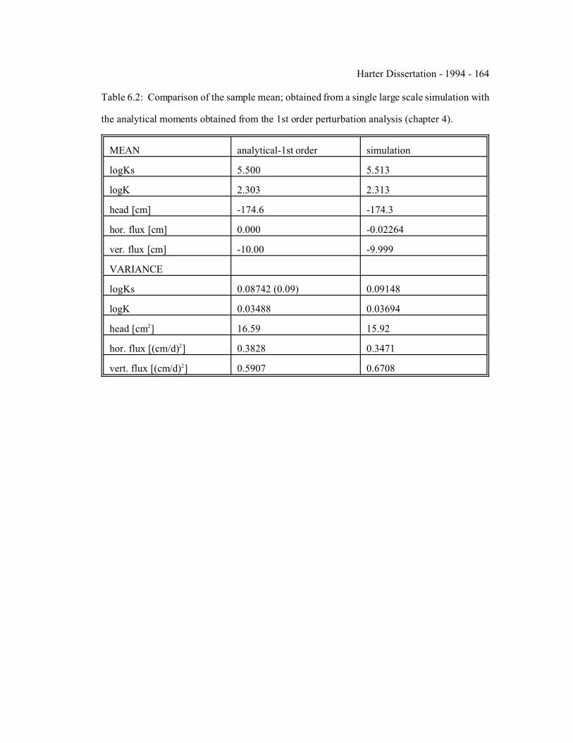
For mass continuity the mean vertical flux must be equal to the specified boundary flux (10
[cm/d]) across the top boundary since no flux occurs across the vertical boundaries. With F =
5.5 and ' = 0.018 [1/cm], the analytical mean pressure head is -174.6 cm, which compares
excellently to the mean pressure head of -174.3 cm in the numerical simulation (Table 6.2).
The mean values of the other output RFVs are also essentially identical with the first order
analytical solution.
The analytical variances are computed from their respective spectral densities by a fast
Fourier transform. For the numerical evaluation of the Fourier transforms, spectral density
functions are calculated on a 10242 grid such that its transform, the covariance function has a
resolution of 11 points per correlation length 8f and a size of 102.4 8f in each direction (see
chapter 4). The exponential input covariance function is also computed as a FFT of its
analytical spectral density function to assess the accuracy of the numerical Fourier transform.
The variance obtained for logKs through the FFT is 3% below the fully analytical equivalent,
which was specified to be 0.09. The accuracy does not improve significantly by increasing the
number of points per correlation length or by increasing the size of the FFT domain. Other
FFT-analytical solutions from the 1st order perturbation analysis for this verification case are
assumed to have a similar margin of accuracy.
Table 6.3 shows that the sample variance of logKs (from the random field generator)
is within 1% of the specified variance due to the normalization (6-9). The sample variances
of logK and the vertical flux are 6% and 14% larger than their analytical variances, respectively.
In contrast the head and horizontal flux variances are by 4% and 9% lower, respectively, than

Harter Dissertation - 1994 - 147
the analytically determined variances. Given the small error of the numerical Fourier transform
the remaining 5% to 10% variability in the sample variance must be attributed to sample error.
Recall that the 2002 samples are not mutually independent and the sample size must therefore
be considered limited.
The horizontal and vertical sample autocorrelation functions are shown in Figure 6.4
together with the analytically derived autocorrelation functions. The autocorrelation function
is obtained from the covariance function by dividing the covariance with its variance. For short
separation distances (>' < 2, where >' = >/8logKs) the sample correlation of logKs is in excellent
agreement with the analytical exponential correlation function. At larger >' the sample
correlation in this realization is weaker than expected from the ensemble (analytical) correlation
function. This is due to the proportionally smaller sample size from which the correlation is
computed as the separation distance increases (Yevjevich, 1972). The smaller sample sizes are
associated with larger sampling errors.
A similarly good agreement at shorter separation distances is seen for the correlation
functions of the unsaturated hydraulic conductivity logK and the horizontal flux qh. In contrast,
the correlation functions of the head and the vertical flux are significantly different from the
ensemble correlation functions even at short lag distances. Since the size and discretization of
the FFT domain in the evaluation of the spectral density function is sufficiently accurate, the
difference between the ensemble and sample correlation functions must be attributed to sample
errors in the simulation. The error of the numerical results is likely due to the limited size of
the simulation domain. Both the horizontal and vertical head ensemble correlation functions
and the vertical ensemble correlation of vv have very long correlation lengths relative to the
total domain length. The total domain length both vertically and horizontally is 20 8f. The
vertical and horizontal correlation lengths of the head and the horizontal correlation length of
qv are three to five times larger than for logKs. The domain length is therefore only about six
times the correlation length of the head. Since the deterministic flux boundaries increase the
variance of the head near the boundary (Rubin and Dagan, 1989) it is not surprising to see a

Harter Dissertation - 1994 - 148
generally shorter correlation length in the sample correlation functions of the head and the
vertical velocity.
Apart from the effects of the limited domain size, the simulations are in excellent
agreement with the analytical solutions. The results confirm that the numerical model gives
sufficiently accurate solutions under a conservative grid-design. Inaccuracies stem from the
limited size of the sample domain given the relatively strong and far-reaching correlation of the
head and the vertical velocity.
6.4.3. Grid-Design Sensitivity Analysis
6.4.3.1 Effects on the 1st Moment (Mean)
The analysis focuses on the sensitivity of the head, flux, and unsaturated hydraulic
conductivity moments with respect to the various design parameters. Figure 6.5 depicts the
sample means of both the input and the output random fields as a function of "g 8f. "g is given
as input parameter. 8f is directly obtained from the random field sample. This is done in an
attempt to minimize the impact of varying sample error (6.4.1) occurring due to different relative
domain lengths. The correlation length 8 of all stochastic variables is computed from the sample
covariance functions (Yevjevich, 1972) by iteratively solving the equation:
Cov(8) = F² e-1 (6-12)
This definition of the correlation length 8 coincides with the definition of the integral scale if
the sample correlation satisfies an exponential correlation function.
The mean values for the input parameters are fairly constant. They show some sample
variation due to the different sizes of the random fields generated. Of the output parameters the
horizontal mean flux <qh>, the vertical mean flux <qv>, and the mean of the unsaturated
hydraulic conductivity <logK> are constant and independent of the grid-size chosen if )x �16
cm. The mean head varies significantly depending on the grid-design but also between Monte
Carlo runs of the same grid-design. For elements larger than 162 [cm2], all sample mean values

Harter Dissertation - 1994 - 149
are decreasing. The only exception is <logKs>, the independent parameter, and <qh>, which
always is close to 0. In particular the mean vertical flux <qv> decreases significantly at large
element lengths although it shows very little sample variation at all for smaller elements. Since
the flux at the top boundary is specified as 10 [cm/d] and no flux occurs across the vertical
boundaries, the decrease in the mean vertical flux rate is an indication of significant numerical
mass balance problems. For elements with )x = 256 [cm] the decrease in mean vertical flux is
more than 20% of the specified flux rate at the top boundary. For the same element size, the
mean head decreases by 15 cm or 30% of the observed standard deviation.
The first order approximations of the head disagree even for small element sizes. The
first order mean head is 174.6 [cm] (see section 6.4.2), while the numerically obtained mean
heads range between 150 and 165 [cm] (based on computations with element lengths of 16 [cm]
and less). While the variance of the output RFVs (unsaturated hydraulic conductivity and head)
is relatively small, the large variance of the input parameters logKs and log" introduce
significant analytical error into the first order approximations of the mean head. This
demonstrates the limitations of the first order solutions derived in chapter 4 (see also chapter 8).
6.4.3.2 Variance and Covariance
HEAD: The normalized head variance F*²h as a function of "g and 8f is computed in
a form similar to the one suggested by Yeh (1985b, eqn. 26a):

Harter Dissertation - 1994 - 150
(6-13)
The normalized head variance for block-size b' = 1 (b=)x) is shown in Figure 6.6 together with
the analytical function obtained from an evaluation of the first order spectral density of the head.
The first order analytical approximation of the 2nd moments of the head and other output
parameters are computed assuming a mean head of 155 [cm], which is representative for the
mean heads of the numerical computations.
It is assumed that the numerical results for small element size and large 8/b are as
accurate in the high input variance case (grid-design analysis) as in the low input variance
simulation (model verification, Figure 6.4)). Although there are quantitative differences, the
empirical head sample variance follows a stochastic function similar to the analytical variance
function. Figure 6.6 shows that for small values of 8f the first order approximation
overestimates the normalized sample variance of the head, while it largely underestimates F*2h
for large 8f. For block-size b'=1, the choice of the relative correlation length 8' = 8/b has a
consistent influence on F*2h: The larger 8' , the lower the normalized head variance. Doubling
8' decreases the normalized variance of the head by approximately 10% with the only exception
being the case 8/b=40. In other words, the higher resolution of the spatial variability in logKs
and log" leads to a slightly lower head variance relative to the variance of the independent RFV
logKs. It is interesting to note that unlike the mean head values the normalized head variance
does not seem to be significantly altered by large element sizes.
The simulations with block size 2*2el. (b'=2)x) and 4*4el. (b'=4)x) give results very
similar to the single element block simulations (Figure 6.7) regarding the general shape of the
empirical variance function. However, here the relative correlation length 8' has the opposite
effect: The larger the resolution of perturbations (higher 8' ) the larger the normalized head
variance. For 2*2el. blocks the normalized head variance increases by 5% to 10% when
doubling the relative correlation length. For 4*4el. blocks, the same increase in relative

Harter Dissertation - 1994 - 151
correlation length causes a 30% to 40% increase in the normalized head variance. Since a
change in relative correlation length changes the number of random points generated (and hence
the sample size), it is not clear from these results whether the differences are statistically
significant and due to the change in 8' or due to the change in the relative block-size b'.
To assess the statistical significance of the results, a small Monte Carlo simulation is
implemented with b'=)x , 8' = (10, 10) to investigate the variability of the sample statistics.
Figure 6.7 indicates the range of values in the normalized head variance for 90% of the 30
Monte Carlo samples. The large range of values for the normalized head variance is the
combined effect of the variability in sample head, in sample correlation length 8f, and in sample
logKs variance (see (6-13)). The smallest and largest non-normalized sample head variances
differ by a factor of 2. In the Monte Carlo simulation the input 8f is 40 [cm]. The sample 8f
varies from 34 to 57 [cm]. The sample variance of logKs, F2
f, ranges from 3.6 to 4.5. The range
of sample mean head values obtained from each of the Monte Carlo runs is equivalent to
approximately 1/2 the head standard deviation. This shows that a single large field simulation
can only give rough estimates of the head variance. The range of the sample moments is much
larger even than the total range covered by the simulations with different element-, block-, and
correlation length. Hence, the differences for the various choices of element size, relative
correlation length 8f', and block size b' observed for element-lengths not exceeding 32 cm are
statistically of limited significance. For a high level of accuracy, the choice of the relative input
correlation length will certainly have to be considered, but then a single large field realization
even with 40,000 elements is inadequate. A greater statistical significance can only be achieved
by evaluating a large number of Monte Carlo runs and by comparing the results of entire Monte
Carlo simulations rather than those of single large realizations. This is beyond the scope of this
chapter. However, the results for different element size )x but identical resolution 8f' and
block-size b' are directly comparable, since they are based on the same set of random numbers.
For the (output) correlation length 8h of the matric suction head the results are similar:
In general, log8h is linearly proportional to log8f (Figure 6.8). For large element sizes (large 8f)

Harter Dissertation - 1994 - 152
(6-14)
only insignificant deviations from a log-linear relationship are observed. Like Fh2, 8h shows a
dependence on the choice of the relative (input) correlation length 8': As 8' increases from 5
to 40, 8h decreases, independent of the block-size chosen. Comparing the correlation structure
for various block-sizes, it seems that the results are not sensitive to the block-discretization e.g.,
for b = )x and 8 = 10b = 10)x the head correlation is the same as for b = 2)x and 8 = 5b =
10)x. The exact match is mere coincidence, given that the first simulation was based on a
random field of 40,000 numbers, while the latter simulation was based on a random sub-field
of only 10,000 numbers.
FLUX: The simulated normalized empirical flux variances Fq*²:
are approximately 30% to 50% above the theoretical 1st order analytical results if "g8f < 1. The
differences between the numerical and the analytical results increase as "g8f increases. The
normalized vertical flux variance deviates even qualitatively from the stochastic analytical
results at correlation lengths corresponding to element sizes )x > 16 cm indicating large
numerical errors with discretizations in excess of much more than 16 cm. The increase in
vertical flux variance for the larger element sizes coincides with the decrease in the mean
vertical flux, further indicating that the vertical flux moments of all output moments are the most
sensitive to the element size. The actual (non-normalized) vertical flux variance (like the
vertical flux mean) is approximately constant for )x � 16 cm (Figure 6.9).
The horizontal flux variance follows a similar stochastic form as the analytical solution
over the range of all correlation lengths/element sizes. The sensitivity of the flux variances to
element-length )x, block-size b', and relative correlation length 8' is in general slightly smaller
than the sensitivity of the head variance to these parameters. Although not explicitly shown

Harter Dissertation - 1994 - 153
in Figure 6.8, the normalized flux variance of both the vertical and the horizontal flux decreases
as the relative correlation length 8' increases. However, the range of variances obtained from
different random fields in the Monte Carlo simulation again indicates the weak statistical
significance of those results due to the sample error associated with one single large realization
when assessing uncertainty of unsaturated flow.
A plot of the vertical and horizontal correlation length 8qv vs. 8f reveals a very strong
correlation to the input correlation length over most of the range tested. Strong deviations from
a log-linear type correlation between 8qv and 8f occur for )x $ 64 cm (Figure 6.10). Figure
6.11 shows the same results for the horizontal flux qh. Unlike 8qv the numerically determined
correlation length of the horizontal flux 8qh slows rather than accelerates its growth relative to
8f for 8f > 100 cm. The analytically derived 8qv and 8qh show a similar nonlinear dependence.
These results for the correlation length of the two flux components as an integrated
measure of the covariance function are rather independent of the block-size chosen. The block-
size itself has a small influence on the results. Given the range of possible outcomes of the
normalized flux variance from a small Monte Carlo simulation, both the influence of the block-
size and of the relative correlation length are almost negligible.
UNSATURATED K: A plot of the variance of logK against "g8 and a plot of the
correlation length of the unsaturated hydraulic conductivity against the input correlation length
of logKs reveals that the unsaturated hydraulic conductivity are little sensitive to the tested grid-
design options for )x # 32 cm (Figure 6.12a-c). As for other statistical output parameters, the
variation of sample moments within a single Monte Carlo simulation exceeds the variations
observed due to different grid-design. Since the dependence of the logK moments on block size
and relative correlation length is much less than the uncertainty arising from the small sample
size and hence from the variability in the sample moments there is little further insight these
simulations can shed.
As expected, a strong linear dependence exists between 8y and 8f. The shape of the
unsaturated variance function is similar to the vertical flux variance function. Note that the

Harter Dissertation - 1994 - 154
vertical flux has a correlation length approximately equal to the input correlation length, while
the correlation length of the unsaturated hydraulic conductivity is only about half of 8f (Figure
6.12b,c). The analytically determined correlation lengths (1st order) are generally larger than
the numerical ones. Only at large 8f > 32 cm both the horizontal and the vertical correlation
length of logK are above the analytical results and also deviate from the linear correlation with
8f.
6.4.3.3 Rectangular vs. Square Elements
To investigate the numerical effect of the ratio between the horizontal and vertical
length of an element, an anisotropic field is simulated once with rectangular blocks consisting
of several square elements and once with rectangular blocks consisting of a single rectangular
element. Each block consists of only one row of elements in the vertical direction. The block-
side ratios b1/b2 in the five cases examined are 2, 4, and 8. The relative correlation length 8'
is 10 in both the vertical and horizontal directions. Table 6.3 compares several selected results
obtained with the square element solutions vs. the rectangular element solutions. For the block-
size ratios in these examples there is a remarkable agreement between both types of element
shape. The difference in output parameter variance is generally less than 5% of the respective
total variance. While the variance of the unsaturated log hydraulic conductivity is slightly
smaller for square elements than for rectangular elements, all other variances are slightly larger
for square elements than for rectangular elements. The differences in the correlation length are
on the order of 1%. The correlation length of the square elements is always slightly smaller
than for rectangular elements. Overall no particularly strong bias is found associated with
different element shapes.
6.5 Comparison with Other Heterogeneous Flow Simulation Studies
Harter Dissertation - 1994 - 155
The general framework of the numerical experiments is similar to simulations reported
by Hopmans et al. (1989), Ünlü et al.(1990), and Russo (1991). The grid-design analysis not
only allows the assessment of the effect of various design parameters but also sheds some
valuable insight into the stochastic analysis of flow in heterogeneous porous media. In the
following paragraphs the results from section 6.4 are compared with the Monte Carlo
simulation results obtained by the above authors.
Russo (1991) and Russo and Dagan (1991) (referred to here as R&D) simulate and
evaluate an infiltration event in heterogeneous, unsaturated media in two dimensions with a
single large domain simulation. Their computer simulation solves Richards equation with 2, the
water content, instead of the matric potential h as dependent variable. The input RFVs are
generated based on the similar media theory (Warrick et al., 1977), which requires one random
field from which all random input variables are derived (compare to (6-8)). Unlike the
simulations here, their simulation was based on VanGenuchten's constitutive equations for K(2)
and R(2). Their grid-discretization was within the framework tested here ()x=20 cm, )z=2
cm). The simulation was based on a grid with just over 30,000 nodes with a relative domain size
d' =(15, 80) in the horizontal and vertical direction, respectively. Since the resulting correlation
length of the water content is similar to the input correlation of the scaling factor, the simulation
results of the water content moments have less sampling error than the head moments in the
simulations implemented here. But no attempt is made to characterize the sample variance of
either the input or the output stochastic sample parameters.
In their analysis R&D suggest that
(F² 8)y = (F² 8)f (6-15)
reasoning that under unsaturated conditions the correlation length of the conductivity decreases
and the variance increases. Clearly, the simulations here demonstrate that the relationship does
not necessarily hold. R&D concluded that the unsaturated hydraulic conductivity variance
increases reciprocal to the decrease in correlation length as the soil dries out. However, the
behavior of F²y among others depends primarily on the set of unsaturated hydraulic conductivity
Harter Dissertation - 1994 - 156
functions generated and on the mean hydraulic head in the simulation. This is true for both
Gardner's and VanGenuchten's expression of K(h) and will be determined by the mean and
variance chosen for the parameters in the K(h) expression. Field evidence qualitatively supports
these findings (White and Sully, 1992). In the simulations described above F²y is smaller than
the variance for the saturated hydraulic conductivity F²f: The correlation of f and log" causes
a continuous decrease of the unsaturated conductivity variance as the mean head decreases until
it reaches a minimum near hmin = -1/("g.) (see Figure 6.13). At heads drier than hmin the
unsaturated conductivity variance increases with decreasing head. While the reduction of F²y
is an artifact of the selected model, it should be understood that parameters are generally chosen
to fit measured data with the K(h) function. In particular, if Gardner's exponential expression
is chosen, the parameter logKs should not be mistaken for the actual saturated hydraulic
conductivity. Gardner's function is known to work well only for a limited range of suction
values. If a wide range of h is expected to occur during the simulations, VanGenuchten's or
other K(h) relations may be more satisfying. In general, however, a statement like (6-15) is not
warranted given the strong dependence of F²y on the K(h) function.
As a consequence of the hypothesis (6-15), R&D also discuss the possibility that
unsaturated transport variability may be governed by similar laws as saturated transport due to
the fact that the "Lagrangian analysis [...] is of general nature and applies to saturated and
unsaturated flow as well." In particular they find for their simulation, that
Fqv2/<qv>² 8qv = F²f 8f (6-16)
The results in section 6.4 partially supports their conclusion. Indeed remarkably close
agreement with (6-16) is found if the variance and correlation length of f=logKs is replaced with
the variance and correlation length of y=logK (Figure 6.14). However, (6-16) does not hold for
logKs as suggested by R&D. This precludes an a priori determination of the longitudinal
dispersivity from F²f and 8f alone. A linear regression curve through the experimental values
also exhibits a slope slightly larger than 1, which does not seem to be caused by the larger )x
alone (see the case, where b = 1)x).

Harter Dissertation - 1994 - 157
A further hypothesis tested by R&D suggests that according to theoretical results
suggested originally for saturated flow, the unsaturated flux moments are characterized
approximately by:
CVqz² = Fqv2/<qz>² = 0.375 F²f (6-17)
In neither Russo's nor the simulations in 6.4 does this particular relationship hold. But if F²logKs
is again replaced with F²logK the agreement between the numerical results and (6-21) is quite
good: In the simulations of section 6.4 CVqz²/F²logK varies from 0.24 to 0.31 for the simulations
with single element blocks, from 0.25 to 0.40 for 2*2 element-blocks, and from 0.28 to 0.34 for
the 4*4 element blocks. This supports the hypothesis that the stochastic theory developed for
the saturated velocity field may hold for the unsaturated field, with logK replacing logKs (Figure
6.15) (see also chapter 9).
The results presented here are also in agreement with some of the findings of Hopmans
et al. (1988) (referred to here as Hopmans), who simulated 2-D infiltration into one- and two-
layered soils. In their simulations of the one-layered case, the simulated soil consists of a set
of random soil property block-columns, each of which is subdivided into homogeneous (finite
difference) elements. They find that the head values converged quickly to the ensemble
moments. Only 10 Monte Carlo simulations with 50 random soil columns (approximately
corresponding to a single realization with 500 random soil columns) were needed to achieve
convergence, a result that is in clear contrast with the findings of section 6.4. As shown
previously even a single realization of 40,000 random blocks may not be considered to give
results of the accuracy reported by Hopmans. The reason for the apparent discrepancy between
Hopmans results and those reported here are the following: (1.) The bottom boundary condition
in Hopmans simulation is fixed with respect to the head, thereby greatly reducing the head
variance in most of the simulation domain. (2.) Hopmans' random fields are random only in the
horizontal direction. The variance in Hopmans simulation varies between 80 and 400 cm2
compared to a range from less than 5 cm2 to more than 1000 cm2 in the simulations presented
here. In contrast to the strong horizontal head correlation of the simulations in this study, the

Harter Dissertation - 1994 - 158
correlation length in Hopmans' simulation was only slightly larger than the input correlation
length and did not exceed 3 )x or 1/15 of the domain size in the horizontal direction (Hopmans
et al, 1988, Figure 5).
Hopmans used correlation lengths (in the definition of (6-12)) of 2 blocks and 4 blocks.
Like in the simulations of this study, a small but discernable difference was found in the head
correlation length that might be attributed to the better resolution of the heterogeneous
properties: Their table 5 also indicates a slight decrease in the correlation length of the head as
the relative input correlation length increases.
The results in 6.4 regarding the stability of the mean head and flux confirm similar
findings of Ünlü et al. (1990) (here referred to as Ünlü). Their one-dimensional, vertical,
transient flow simulations showed a similar behavior of the head and flux variance as a function
of the input variance as Hopmans simulations and the simulations ins section 6.4. Furthermore,
the simulations in this study confirm the conclusion of Ünlü, that the flux variance in mean
flow direction increases, if the correlation length in mean flow direction increases, while the
vertical flux variance decreases, if the correlation length in the horizontal direction increases:
In the simulations with varying element-width )x2, but element-"thickness" )x1 (and
consequently a change of 8x2 but not of 8x1) the simulations with larger 8x2 have a significantly
smaller variance in qx1, while the variance of qx2 increases. In all other simulations, the
simultaneous change in width and thickness of the element (to keep the square form) and hence
in 8 caused a decrease in F²qh, but an increase in F²qv for any constant 8/b and b/)x1. Although
discernable, the increase in the vertical flux variance is by far not as drastic as observed in the
1-dimensional simulations of Ünlü. This is expected due to the higher degree of freedom in the
flow-path for the 2-D simulations (see also Yeh, 1985a).
6.6 Conclusion and Summary
The previous analysis of several dozen flow simulations with varying element-size,
Harter Dissertation - 1994 - 159
block-size, and correlation-length allows valuable insight into the accuracy of numerical
stochastic solutions and its dependence on grid-design. The simulation further sheds some light
on previous analyses by various authors.
As part of the model verification the numerical solutions for the stochastic moments of
the head and flux (mean, variance, and covariance) are found to compare well with the analytical
results for 2-D flow that were derived in chapter 4. The only disagreement found between
analytical and numerical results are the covariance functions of the head and the vertical flux.
Both the head and the vertical flux have very long correlation lengths, several times longer than
the input correlation length 8f. The size of the domain (200 by 200 elements or 20 by 20
correlation lengths) is found to be inadequate to unbiasedly sample the head and vertical flux.
As a result the numerical covariance functions are of significantly shorter correlation length than
the analytical covariances for the head and the vertical velocity.
The grid design sensitivity analysis was implemented with parameters chosen to be
representative of field conditions. The conservative grid-design simulation results served as
comparative basis for the sensitivity analysis. Since the input parameters have a large variance,
the analytical solutions derived in chapter 4 cannot serve as a direct verification tool for the grid
design sensitivity analysis. Instead it may serve as a guideline only. Indeed, the moments of
the numerical simulation significantly differ from the analytically determined moments, even
for the same conservatively chosen grid-design. But the general qualitative dependency between
stochastic input and output parameters was found to be similar.
The element-size was found to have little influence on the head solution accuracy as
long as 32 cm thickness and width was not exceeded. Numerical oscillations significantly
distort the head and unsaturated hydraulic conductivity moments only if simulations are based
on element-sizes of 64 cm and larger. The vertical flux moments are more sensitive to the grid-
design than the head moments and require an element size of 16 cm or less in the vertical
direction. A grid-Peclet number ")x < 2, derived for the quasi-linear form of Richards
equation, gives a very safe margin if it is strictly applied such that the condition is met for all

Harter Dissertation - 1994 - 160
elements. Based on the findings of section 6.4 a weaker grid-Peclet number restriction can be
formulated:
"g)x < 0.5 (6-18)
where "g is the geometric mean of ". This criterion is simple to implement, gives larger
freedom in the choice of the element-size and still provides accurate solutions. For most
practical purposes, this allows grid-sizes of up to 20 cm and more in the vertical direction. The
element size in the horizontal direction is by far not as critical, and horizontal element lengths
of e.g. 4 cm and 32 cm give identical results.
The subdiscretization into multi-element blocks for better resolution of the nonlinear
head variations gave little improvement in the accuracy of the solutions. The differences to the
simulations with single-element blocks were subtle and statistically of little significance. If
b=)x is sufficiently small to give a good resolution of the heterogeneities (i.e. b/8 # 0.1), and
if )x satisfies the grid-Peclet criterion to avoid oscillations, the error introduced by linear head
interpolation between element nodes is reduced sufficiently to be neglected.
The simulations have shown that the choice of a larger relative correlation length has
a discernable albeit small effect on the head and flux variance and covariance: With large 8/b
the stronger coherence of random input parameters reduces the discrete jumps in hydraulic
properties between neighboring blocks. Hence, the nonlinearity in the matric potential field
decreases, while its numerical approximation improves. As a result the output variance of the
head tends to increase due to a higher resolution of the perturbations and the output head
correlation length decreases. In contrast, the flux variance decreases as the perturbation
resolution increases. The differences have a weak statistical significance but are in accordance
with findings by Hopmans et al. (1988).
By comparing several single large realizations it was found that simulations, which are
based on a singe large realization, give stochastic results that are associated with considerable
sampling error. Although only results for a limited number of Monte Carlo realizations are
available, the variations of the sample correlation lengths and sample variances of head and flux

Harter Dissertation - 1994 - 161
indicate that a single realization with 104 - 105 elements and a side-length of 20 8f does give
results with a sampling error of up to a factor 2.
With respect to previously implemented research, the simulations confirm the hypothesis
by Russo and Dagan (1991), that the unsaturated velocity field may be subject to the same
stochastic processes formulated for the saturated case. By consistently replacing the moments
of logKs with the moments of logK, it was shown that the Lagrangian unsaturated flux moments
presented in Russo and Dagan (1991) are related to the unsaturated hydraulic conductivity
moments in a manner very similar to that found under saturated condition. The simulations in
this chapter are not considered a complete proof of their hypothesis because other factors, like
the infiltration rate and the geometric mean of ", may strongly influence the results as well. Here
these parameters were kept constant. It would be particularly interesting to investigate the
proposed relationships for water movement in dry soils. Most importantly, however, it is also
shown that their assumption (6-15) does not generally hold. In contrast to the suggestion by
Russo and Dagan (1991), it is therefore not possible to derive the moments of the flux field
directly from the moments of the input random field of logKs.
Further research is certainly necessary to obtain a better understanding of numerical
grid-design in stochastic simulations of unsaturated flow. This research has not addressed the
impact of the infiltration rate on grid-design or the effect of different constitutive functions and
constitutive parameters. The soil flow simulations only addressed accuracy for steady-state
conditions in a relatively moist soil. The results underline the necessity of a careful grid-design
evaluation to avoid numerical errors but also indicate that much more rigorous Monte Carlo
simulations are necessary to accurately assess the impact of grid-design. At computation times
exceeding 6 to 10 hours even on a dedicated workstation such Monte Carlo simulations are very
limited in the number of realizations. The next chapter will introduce a numerical technique that
accelerates the numerical computation time by up to two orders of magnitude. With such
improvements in the computational techniques, Monte Carlo simulations can easily be
implemented with hundreds of realizations. Chapter 8 will present the analysis of unsaturated

Harter Dissertation - 1994 - 162
flow with multiple realization Monte Carlo simulations.

Harter Dissertation - 1994 - 163
Table 6.1: Non-variable input parameters common to all simulations of the model verification
and grid design analysis.
input parameter model verification grid design analysis
mean logKs 5.5 5.5
variance logKs 0.09 4.0
mean log" -4.0 -4.0
variance log" 0.0009 0.25
saturated water content 0.3 0.3
residual water content 0.3 0.3
Harter Dissertation - 1994 - 164
Table 6.2: Comparison of the sample mean; obtained from a single large scale simulation with
the analytical moments obtained from the 1st order perturbation analysis (chapter 4).
MEAN analytical-1st order simulation
logKs 5.500 5.513
logK 2.303 2.313
head [cm] -174.6 -174.3
hor. flux [cm] 0.000 -0.02264
ver. flux [cm] -10.00 -9.999
VARIANCE
logKs 0.08742 (0.09) 0.09148
logK 0.03488 0.03694
head [cm2] 16.59 15.92
hor. flux [(cm/d)2] 0.3828 0.3471
vert. flux [(cm/d)2] 0.5907 0.6708

Harter Dissertation - 1994 - 165
Table 6.3: Comparison of the sample variance and correlation length for rectangular elements
(1st row) and square elements (2nd row). Each column represents a different block-size
indicated in the top row. All units are based on [cm] and [days].
rectang./square 4 x 2 cm2 8 x 2 cm2 16 x 2
cm2
8 x 4 cm2 16 x 4
cm2
32 x 4
cm2
F2 logK 0.440 0.410 0.388 0.387 0.353 0.339
0.439 0.406 0.385 0.385 0.350 0.338
F2 head 35.9 61.1 103 78.1 134 22.2
36.4 54.6 104 78.5 128 223 .1
F2 qh 5.20 4.85 4.07 4.61 3.95 3.08
5.38 5.12 4.46 4.78 4.19 3.39
F2 qv 8.85 6.22 3.74 8.16 5.28 2.72
8.85 6.73 4.12 8.17 5.74 3.07
8 logKs 31.8 63.6 127 .2 63.6 127 .2 254
31.8 63.6 127 .2 63.6 127 .2 254
8 logK 14.7 28.6 57.1 27.2 532 .6 110
14.7 28.5 57.3 27.2 523 .9 111
8 head 68.0 75.8 106 83.1 114 .4 183
68.7 66.3 105 83.3 111 .3 181
8 qh 14.3 23.1 37.9 26.7 42.7 73.0
14.1 23.+ 37.2 26.4 42.5 71.5
8 qv 10.0 17.4 27.1 19.0 31.3 48.8
10.2 17.8 26.1 19.3 31.9 45.4

Harter Dissertation - 1994 - 166
Figure 6.1: Matric potential distribution in a 3-layered soil column. Layer 1 is a very lowpermeable soil with small ". Permeability and ".increase with each of thesubsequent two-layers. Inversely, the nonlinear portion of the capillary fringedecreases. Layer 3 requires smaller discretization than layer 2 or layer 1 toaccurately capture the nonlinear portion of the matric potential curve.
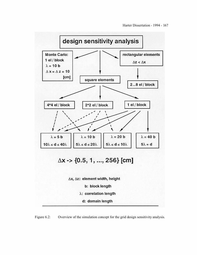
Harter Dissertation - 1994 - 167
Figure 6.2: Overview of the simulation concept for the grid design sensitivity analysis.

Harter Dissertation - 1994 - 168
Figure 6.3: Two-point autocorrelation function of the random field for various relativedomain sized D/8. The absolute domain size is 200 by 200 grid points. Theautocorrelation function is computed by spatial averaging for lag-distances upto half the length of the random field.

Fig
ure
6.4:
The
oret
ical
aut
ocor
rela
tion
fun
ctio
n in
com
pari
son
wit
h th
e nu
mer
ical
sam
ple
auto
corr
elat
ion
of t
he i
nput
and
outp
ut R
FV
s.
Harter Dissertation - 1994 - 169

Fig
ure
6.5
:
Sam
ple
mea
n o
f in
pu
t an
d o
utp
ut
RF
Gs
for
each
rea
liza
tio
n a
s a
fun
ctio
n o
f th
e sa
mp
le c
orr
elat
ion
len
gth
8 f or
f =
logK
s giv
en
" g = 0
.01
8 [
cm
-1 ].
Harter Dissertation - 1994 - 170

Harter Dissertation - 1994 - 171
F i g u r e6.6: Normalized head variance as a function of "g 8f, where 8f is the sample correlation
length of f = logKs. Only simulations with block-size b=)x are shown.

Fig
ure
6.7
:
Th
e n
orm
aliz
ed h
ead
var
ian
ce a
s sh
ow
n i
n F
igu
re 6
.6,
bu
t fo
r va
rio
us
blo
ck-s
izes
b:
b=
) x (1
elem
ent/
blo
ck),
b=
2
) x (2
*2
ele
men
ts/b
lock
), b
=4
) x (4
*4
ele
men
ts/b
lock
).
Harter Dissertation - 1994 - 172

Harter Dissertation - 1994 - 173
F igure 6.8: Vertical correlation length of the sample head values for each simulation.

Harter Dissertation - 1994 - 174
Figure 6.9: Normalized variances of the vertical (a) and horizontal (b) flux. Results fromall simulations and from 7 of the 30 Monte Carlo realizations are plotted. Thestraight line below the numerical data is a first order perturbation solution.

Harter Dissertation - 1994 - 175
Figure 6.10: Vertical (top) and horizontal (bottom) sample correlation length of the verticalvelocity. The solid line is obtained from the first-order perturbation analysis.

Harter Dissertation - 1994 - 176
Figure 6.11: Vertical (a) and horizontal (b) sample correlation length of the horizontalvelocity. The solid line indicates the first order perturbation solution.

Harter Dissertation - 1994 - 177
Figure 6 . 1 2 :Variance (a), vertical (b) and horizontal (c) sample correlation length of the unsaturatedhydraulic conductivity y = log K. The solid lines represent the first-order perturbationsolutions derived in chapter 4.

Harter Dissertation - 1994 - 178
Figure 6.13: Envelope of all possible unsaturated hydraulic conductivity curves in run 1 ofthe log"-case Monte Carlo simulation.

Harter Dissertation - 1994 - 179
Figure 6.14: The Lagrangian flux field equation (6-16) using sample parameters of thesaturated hydraulic conductivity (top) and of the unsaturated hydraulicconductivity (bottom).

Harter Dissertation - 1994 - 180
Figure 6.15: Squared coefficient of variation of the vertical flux compared to 3/8 Ff2 (top)
and to 3/8 Fy2 (bottom); see equation 6-17.