6 metropolis{hastings algorithms - .net framework

6

Metropolis–Hastings Algorithms

“How absurdly simple!”, I cried.“Quite so!”, said he, a little nettled. “Every problem becomes verychildish when once it is explained to you.”

Arthur Conan DoyleThe Adventure of the Dancing Men

Reader’s guide

This chapter is the first of a series of two on simulation methods based on Markovchains. Although the Metropolis–Hastings algorithm can be seen as one of themost general Markov chain Monte Carlo (MCMC) algorithms, it is also one of thesimplest both to understand and explain, making it an ideal algorithm to startwith.

This chapter begins with a quick refresher on Markov chains, just the ba-sics needed to understand the algorithms. Then we define the Metropolis–Hastings algorithm, focusing on the most common versions of the algorithm.We end up discussing the calibration of the algorithm via its acceptance rate inSection 6.5.

C.P. Robert, G. Casella, Introducing Monte Carlo Methods with R, Use R, DOI 10.1007/978-1-4419-1576-4_6, © Springer Science+Business Media, LLC 2010

168 6 Metropolis–Hastings Algorithms

6.1 Introduction

For reasons that will become clearer as we proceed, we now make a fundamen-tal shift in the choice of our simulation strategy. Up to now we have typicallygenerated iid variables directly from the density of interest f or indirectlyin the case of importance sampling. The Metropolis–Hastings algorithm in-troduced below instead generates correlated variables from a Markov chain.The reason why we opt for such a radical change is that Markov chains carrydifferent convergence properties that can be exploited to provide easier pro-posals in cases where generic importance sampling does not readily apply. Forone thing, the requirements on the target f are quite minimal, which allowsfor settings where very little is known about f . Another reason, as illustratedin the next chapter, is that this Markov perspective leads to efficient decom-positions of high-dimensional problems in a sequence of smaller problems thatare much easier to solve.

Thus, be warned that this is a pivotal chapter in that we now introduce atotally new perspective on the generation of random variables, one that hashad a profound effect on research and has expanded the application of statis-tical methods to solve more difficult and more relevant problems in the lasttwenty years, even though the origins of those techniques are tied with thoseof the Monte Carlo method in the remote research center of Los Alamos dur-ing the Second World War. Nonetheless, despite the recourse to Markov chainprinciples that are briefly detailed in the next section, the implementation ofthese new methods is not harder than those of earlier chapters, and there isno need to delve any further into Markov chain theory, as you will soon dis-cover. (Most of your time and energy will be spent in designing and assessingyour MCMC algorithms, just as for the earlier chapters, not in establishingconvergence theorems, so take it easy!)

6.2 A peek at Markov chain theory

� This section is intended as a minimalist refresher on Markov chains in or-der to define the vocabulary of Markov chains, nothing more. In case youhave doubts or want more details about these notions, you are stronglyadvised to check a more thorough treatment such as Robert and Casella(2004, Chapter 6) or Meyn and Tweedie (1993) since no theory of con-vergence is provided in the present book.

A Markov chain {X(t)} is a sequence of dependent random variables

X(0), X(1), X(2), . . . , X(t), . . .

such that the probability distribution of X(t) given the past variables dependsonly on X(t−1). This conditional probability distribution is called a transitionkernel or a Markov kernel K; that is,

6.2 A peek at Markov chain theory 169

X(t+1) | X(0), X(1), X(2), . . . , X(t) ∼ K(X(t), X(t+1)) .

For example, a simple random walk Markov chain satisfies

X(t+1) = X(t) + εt ,

where εt ∼ N (0, 1), independently of X(t); therefore, the Markov kernelK(X(t), X(t+1)) corresponds to a N (X(t), 1) density.

For the most part, the Markov chains encountered in Markov chain MonteCarlo (MCMC) settings enjoy a very strong stability property. Indeed, a sta-tionary probability distribution exists by construction for those chains; that is,there exists a probability distribution f such that ifX(t) ∼ f , thenX(t+1) ∼ f .Therefore, formally, the kernel and stationary distribution satisfy the equation

(6.1)∫XK(x, y)f(x)dx = f(y).

The existence of a stationary distribution (or stationarity) imposes a pre-liminary constraint on K called irreducibility in the theory of Markov chains,which is that the kernel K allows for free moves all over the stater-space,namely that, no matter the starting value X(0), the sequence {X(t)} has apositive probability of eventually reaching any region of the state-space. (Asufficient condition is that K(x, ·) > 0 everywhere.) The existence of a station-ary distribution has major consequences on the behavior of the chain {X(t)},one of which being that most of the chains involved in MCMC algorithmsare recurrent, that is, they will return to any arbitrary nonnegligible set aninfinite number of times.

Exercise 6.1 Consider the Markov chain defined by X(t+1) = %X(t) +εt, whereεt ∼ N (0, 1). Simulating X(0) ∼ N (0, 1), plot the histogram of a sample of X(t)

for t ≤ 104 and % = .9. Check the potential fit of the stationary distributionN (0, 1/(1− %2)).

In the case of recurrent chains, the stationary distribution is also a limitingdistribution in the sense that the limiting distribution of X(t) is f for almostany initial value X(0). This property is also called ergodicity, and it obviouslyhas major consequences from a simulation point of view in that, if a givenkernel K produces an ergodic Markov chain with stationary distribution f ,generating a chain from this kernel K will eventually produce simulationsfrom f . In particular, for integrable functions h, the standard average

(6.2)1T

T∑t=1

h(X(t)) −→ Ef [h(X)] ,

which means that the Law of Large Numbers that lies at the basis of MonteCarlo methods (Section 3.2) can also be applied in MCMC settings. (It is thensometimes called the Ergodic Theorem.)


We won’t dabble any further into the theory of convergence of MCMCalgorithms, relying instead on the guarantee that standard versions of thesealgorithms such as the Metropolis–Hastings algorithm or the Gibbs samplerare almost always theoretically convergent. Indeed, the real issue with MCMCalgorithms is that, despite those convergence guarantees, the practical imple-mentation of those principles may imply a very lengthy convergence time or,worse, may give an impression of convergence while missing some importantaspects of f , as discussed in Chapter 8.

There is, however, one case where convergence never occurs, namely when,in a Bayesian setting, the posterior distribution is not proper (Robert, 2001)since the chain cannot be recurrent. With the use of improper priors f(x)being quite common in complex models, there is a possibility that the prod-uct likelihood × prior, `(x) × f(x), is not integrable and that this problemgoes undetected because of the inherent complexity. In such cases, Markovchains can be simulated in conjunction with the target `(x)×f(x) but cannotconverge. In the best cases, the resulting Markov chains will quickly exhibitdivergent behavior, which signals there is a problem. Unfortunately, in theworst cases, these Markov chains present all the outer signs of stability andthus fail to indicate the difficulty. More details about this issue are discussedin Section 7.6.4 of the next chapter.

Exercise 6.2 Show that the random walk has no stationary distribution. Givethe distribution of X(t) for t = 104 and t = 106 when X(0) = 0, and deduce thatX(t) has no limiting distribution.

6.3 Basic Metropolis–Hastings algorithms

The working principle of Markov chain Monte Carlo methods is quite straight-forward to describe. Given a target density f , we build a Markov kernel Kwith stationary distribution f and then generate a Markov chain (X(t)) usingthis kernel so that the limiting distribution of (X(t)) is f and integrals can beapproximated according to the Ergodic Theorem (6.2). The difficulty shouldthus be in constructing a kernel K that is associated with an arbitrary densityf . But, quite miraculously, there exist methods for deriving such kernels thatare universal in that they are theoretically valid for any density f !

The Metropolis–Hastings algorithm is an example of those methods.(Gibbs sampling, described in Chapter 7, is another example with equally uni-versal potential.) Given the target density f , it is associated with a workingconditional density q(y|x) that, in practice, is easy to simulate. In addition, qcan be almost arbitrary in that the only theoretical requirements are that theratio f(y)/q(y|x) is known up to a constant independent of x and that q(·|x)has enough dispersion to lead to an exploration of the entire support of f . Once

6.3 Basic Metropolis–Hastings algorithms 171

again, we stress the incredible feature of the Metropolis–Hastings algorithmthat, for every given q, we can then construct a Metropolis–Hastings kernelsuch that f is its stationary distribution.

6.3.1 A generic Markov chain Monte Carlo algorithm

The Metropolis–Hastings algorithm associated with the objective (target)density f and the conditional density q produces a Markov chain (X(t))through the following transition kernel:

Algorithm 4 Metropolis–HastingsGiven x(t),

1. Generate Yt ∼ q(y|x(t)).2. Take

X(t+1) =

{Yt with probability ρ(x(t), Yt),x(t) with probability 1− ρ(x(t), Yt),

where

ρ(x, y) = min{f(y)f(x)

q(x|y)q(y|x)

, 1}.

A generic R implementation is straightforward, assuming a generator forq(y|x) is available as geneq(x). If x[t] denotes the value of X(t),

> y=geneq(x[t])> if (runif(1)<f(y)*q(y,x[t])/(f(x[t])*q(x[t],y))){+ x[t+1]=y+ }else{+ x[t+1]=x[t]+ }

since the value y is always accepted when the ratio is larger than one.The distribution q is called the instrumental (or proposal or candidate)

distribution and the probability ρ(x, y) the Metropolis–Hastings acceptanceprobability. It is to be distinguished from the acceptance rate, which is theaverage of the acceptance probability over iterations,

ρ = limT→∞

1T

T∑t=0

ρ(X(t), Yt) =∫ρ(x, y)f(x)q(y|x) dydx.

This quantity allows an evaluation of the performance of the algorithm, asdiscussed in Section 6.5.


While, at first glance, Algorithm 4 does not seem to differ from Algorithm2, except for the notation, there are two fundamental differences between thetwo algorithms. The first difference is in their use since Algorithm 2 aims atmaximizing a function h(x), while the goal of Algorithm 4 is to explore thesupport of the density f according to its probability. The second differenceis in their convergence properties. With the proper choice of a temperatureschedule Tt in Algorithm 2, the simulated annealing algorithm converges tothe maxima of the function h, while the Metropolis–Hastings algorithm isconverging to the distribution f itself. Finally, modifying the proposal q alongiterations may have drastic consequences on the convergence pattern of thisalgorithm, as discussed in Section 8.5.

Algorithm 4 satisfies the so-called detailed balance condition,

(6.3) f(x)K(y|x) = f(y)K(x|y) ,

from which we can deduce that f is the stationary distribution of the chain{X(t)} by integrating each side of the equality in x (see Exercise 6.8).

That Algorithm 4 is naturally associated with f as its stationary distribu-tion thus comes quite easily as a consequence of the detailed balance conditionfor an arbitrary choice of the pair (f, q). In practice, the performance of thealgorithm will obviously strongly depend on this choice of q, but considerfirst a straightforward example where Algorithm 4 can be compared with iidsampling.

Example 6.1. Recall Example 2.7, where we used an Accept–Reject algo-rithm to simulate a beta distribution. We can just as well use a Metropolis–Hastings algorithm, where the target density f is the Be(2.7, 6.3) density and thecandidate q is uniform over [0, 1], which means that it does not depend on theprevious value of the chain. A Metropolis–Hastings sample is then generated withthe following R code:

> a=2.7; b=6.3; c=2.669 # initial values> Nsim=5000> X=rep(runif(1),Nsim) # initialize the chain> for (i in 2:Nsim){+ Y=runif(1)+ rho=dbeta(Y,a,b)/dbeta(X[i-1],a,b)+ X[i]=X[i-1] + (Y-X[i-1])*(runif(1)<rho)+ }

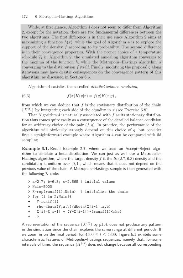
A representation of the sequence (X(t)) by plot does not produce any patternin the simulation since the chain explores the same range at different periods. Ifwe zoom in on the final period, for 4500 ≤ t ≤ 4800, Figure 6.1 exhibits somecharacteristic features of Metropolis–Hastings sequences, namely that, for someintervals of time, the sequence (X(t)) does not change because all corresponding


Fig. 6.1. Sequence X(t) for t = 4500, . . . , 4800, when simulated from theMetropolis–Hastings algorithm with uniform proposal and Be(2.7, 6.3) target.

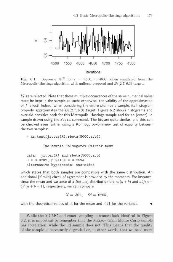
Yt’s are rejected. Note that those multiple occurrences of the same numerical valuemust be kept in the sample as such; otherwise, the validity of the approximationof f is lost! Indeed, when considering the entire chain as a sample, its histogramproperly approximates the Be(2.7, 6.3) target. Figure 6.2 shows histograms andoverlaid densities both for this Metropolis–Hastings sample and for an (exact) iidsample drawn using the rbeta command. The fits are quite similar, and this canbe checked even further using a Kolmogorov–Smirnov test of equality betweenthe two samples:

> ks.test(jitter(X),rbeta(5000,a,b))

Two-sample Kolmogorov-Smirnov test

data: jitter(X) and rbeta(5000,a,b)D = 0.0202, p-value = 0.2594alternative hypothesis: two-sided

which states that both samples are compatible with the same distribution. Anadditional (if mild) check of agreement is provided by the moments. For instance,since the mean and variance of a Be(a, b) distribution are a/(a+ b) and ab/(a+b)2(a+ b+ 1), respectively, we can compare

X̄ = .301 , S2 = .0205 ,

with the theoretical values of .3 for the mean and .021 for the variance. J

While the MCMC and exact sampling outcomes look identical in Figure6.2, it is important to remember that the Markov chain Monte Carlo samplehas correlation, while the iid sample does not. This means that the qualityof the sample is necessarily degraded or, in other words, that we need more


Fig. 6.2. Histograms of beta Be(2.7, 6.3) random variables with density func-tion overlaid. In the left panel, the variables were generated from a Metropolis–Hastings algorithm with a uniform candidate, and in the right panel the randomvariables were directly generated using rbeta(n,2.7,6.3).

simulations to achieve the same precision. This issue is formalized throughthe notion of effective sample size for Markov chains (Section 8.4.3).

In the symmetric case (that is, when q(x|y) = q(y|x)), the acceptance prob-ability ρ(xt, yt) is driven by the objective ratio f(yt)/f(x(t)) and thus even theacceptance probability is independent from q. (This special case is detailed inSection 6.4.1.) Again, Metropolis–Hastings algorithms share the same featureas the stochastic optimization Algorithm 2 (see Section 5.5), namely that theyalways accept values of yt such that the ratio f(yt)/q(yt|x(t)) is increased com-pared with the “previous” value f(x(t))/q(x(t)|yt). Some values yt such thatthe ratio is decreased may also be accepted, depending on the ratio of the


ratios, but if the decrease is too sharp, the proposed value yt will almost al-ways be rejected. This property indicates how the choice of q can impact theperformance of the Metropolis–Hastings algorithm. If the domain explored byq (its support) is too small, compared with the range of f , the Markov chainwill have difficulties in exploring this range and thus will converge very slowly(if at all for practical purposes).

Another interesting property of the Metropolis–Hastings algorithm thatadds to its appeal is that it only depends on the ratios

f(yt)/f(x(t)) and q(x(t)|yt)/q(yt|x(t)) .

It is therefore independent of normalizing constants. Moreover, since all thatmatters is the ability to (a) simulate from q and (b) compute the ratiof(yt)/q(yt|x(t)), q may be chosen in such a way that the intractable partsof f are eliminated in the ratio.

� Since q(y|x) is a conditional density, it integrates to one in y and, assuch, involves a functional term that depends on both y and x as wellas a normalizing term that depends on x, namely q(y|x) = C(x)q̃(x, y).When noting above that the Metropolis–Hastings acceptance probabilitydoes not depend on normalizing constants, terms like C(x) are obviouslyexcluded from this remark since they must appear in the acceptance prob-ability, lest it jeopardize the stationary distribution of the chain.

6.3.2 The independent Metropolis–Hastings algorithm

The Metropolis–Hastings algorithm of Section 6.3.1 allows a candidate distri-bution q that only depends on the present state of the chain. If we now requirethe candidate q to be independent of this present state of the chain (that is,q(y|x) = g(y)), we do get a special case of the original algorithm:

Algorithm 5 Independent Metropolis–HastingsGiven x(t)

1. Generate Yt ∼ g(y).2. Take

X(t+1) =

Yt with probability min{f(Yt) g(x(t))f(x(t)) g(Yt)

, 1}

x(t) otherwise.


This method then appears as a straightforward generalization of theAccept–Reject method in the sense that the instrumental distribution is thesame density g as in the Accept–Reject method. Thus, the proposed valuesYt are the same, if not the accepted ones.

Metropolis–Hastings algorithms and Accept–Reject methods (Section 2.3),both being generic simulation methods, have similarities between them thatallow comparison, even though it is rather rare to consider using a Metropolis–Hastings solution when an Accept–Reject algorithm is available. In particular,consider that

a. The Accept–Reject sample is iid, while the Metropolis–Hastings sample isnot. Although the Yt’s are generated independently, the resulting sampleis not iid, if only because the probability of acceptance of Yt depends onX(t) (except in the trivial case when f = g).

b. The Metropolis–Hastings sample will involve repeated occurrences of thesame value since rejection of Yt leads to repetition of X(t) at time t + 1.This will have an impact on tests like ks.test that do not accept ties.

c. The Accept–Reject acceptance step requires the calculation of the upperbound M ≥ supx f(x)/g(x), which is not required by the Metropolis–Hastings algorithm. This is an appealing feature of Metropolis–Hastings ifcomputing M is time-consuming or if the existing M is inaccurate andthus induces a waste of simulations.

Exercise 6.3 Compute the acceptance probability ρ(x, y) in the case q(y|x) =g(y). Deduce that, for a given value x(t), the Metropolis–Hastings algorithmassociated with the same pair (f, g) as an Accept–Reject algorithm accepts theproposed value Yt more often than the Accept–Reject algorithm.

The following exercise gives a first comparison of Metropolis–Hastings withan Accept–Reject algorithm already used in Exercise 2.20 when both algo-rithms are based on the same candidate.

Exercise 6.4 Consider the target as the G(α, β) distribution and the candidateas the gamma G([α], b) distribution (where [a] denotes the integer part of a).

a. Derive the corresponding Accept–Reject method and show that, when β = 1,the optimal choice of b is b = [α]/α.

b. Generate 5000 G(4, 4/4.85) random variables to derive a G(4.85, 1) sample(note that you will get less than 5000 random variables).

c. Use the same sample in the corresponding Metropolis–Hastings algorithm togenerate 5000 G(4.85, 1) random variables.

d. Compare the algorithms using (i) their acceptance rates and (ii) the estimatesof the mean and variance of the G(4.85, 1) along with their errors. (Hint:Examine the correlation in both samples.)


Fig. 6.3. Histograms and autocovariance functions from a gamma Accept–Reject algorithm (left panels) and a gamma Metropolis–Hastings algorithm (rightpanels). The target is a G(4.85, 1) distribution and the candidate is a G(4, 4/4.85)distribution. The autocovariance function is calculated with the R function acf.

Figure 6.3 illustrates Exercise 6.4 by comparing both Accept–Reject andMetropolis–Hastings samples. In this setting, operationally, the indepen-dent Metropolis–Hastings algorithm performs very similarly to the Accept–Reject algorithm, which in fact generates perfect and independent randomvariables.

Theoretically, it is also feasible to use a pair (f, g) such that a bound M onf/g does not exist and thus to use Metropolis–Hastings when Accept–Reject isnot possible. However, as detailed in Robert and Casella (2004) and illus-trated in the following formal example, the performance of the Metropolis–Hastings algorithm is then very poor, while it is very strong as long assup f/g = M <∞.


Example 6.2. To generate a Cauchy random variable (that is, when f corre-sponds to a C(0, 1) density), formally it is possible to use a N (0, 1) candidatewithin a Metropolis–Hastings algorithm. The following R code will do it:

> Nsim=10^4> X=c(rt(1,1)) # initialize the chain from the stationary> for (t in 2:Nsim){+ Y=rnorm(1) # candidate normal+ rho=dt(Y,1)*dnorm(X[t-1])/(dt(X[t-1],1)*dnorm(Y))+ X[t]=X[t-1] + (Y-X[t-1])*(runif(1)<rho)+ }

When executing this code, you may sometimes start with a large value for X(0),12.788 say. In this case, dnorm(X[t-1]) is equal to 0 because, while 12.788can formally be a realization from a normal N (0, 1), it induces computationalunderflow problems

> pnorm(12.78,log=T,low=F)/log(10)[1] -36.97455

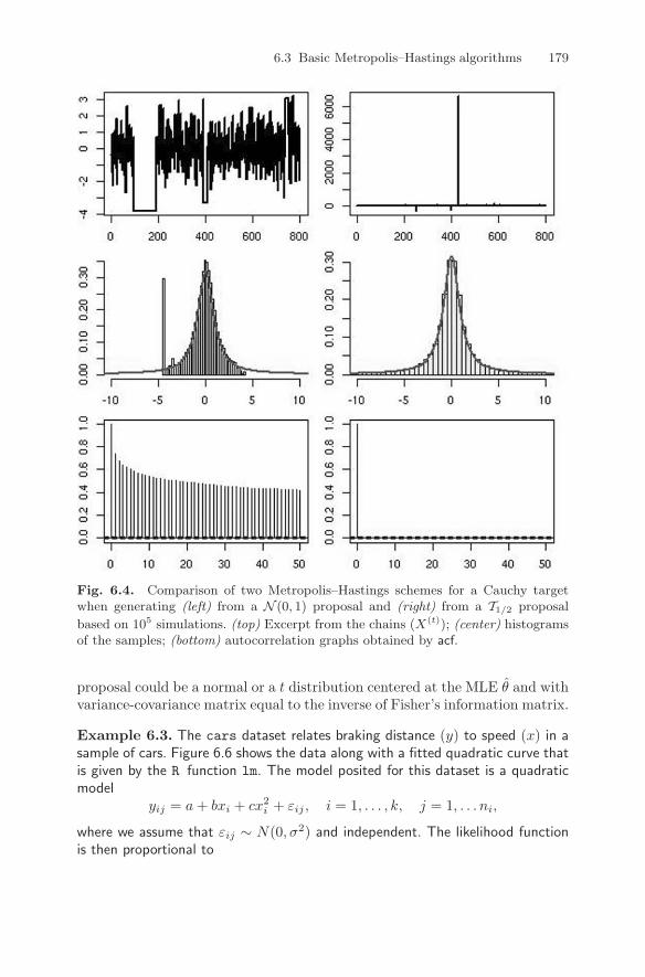
(meaning the probability of exceeding 12.78 is 10−37) and the Markov chainremains constant for the 104 iterations! If the chain starts from a more centralvalue, the outcome will resemble a normal sample much more than a Cauchysample, as shown by Figure 6.4 (center right). In addition, very large values ofthe sequence will be heavily weighted, resulting in long strings where the chainremains constant, as shown by Figure 6.4, the isolated peak in the histogrambeing representative of such an occurrence. If instead we use for the independentproposal g a Student’s t distribution with .5 degrees of freedom (that is, if wereplace Y=rnorm(1) with Y=rt(1,.5) in the code above), the behavior of thechain is quite different. Very large values of Yt may occur from time to time (asshown in Figure 6.4 (upper left)), the histogram fit is quite good (center left),and the sequence exhibits no visible correlation (lower left). If we consider theapproximation of a quantity like Pr(X < 3), for which the exact value is pt(3,1)(that is, 0.896), the difference between the two choices of g is crystal clear inFigure 6.5, obtained by

> plot(cumsum(X<3)/(1:Nsim),lwd=2,ty="l",ylim=c(.85,1)).

The chain based on the normal proposal is consistently off the true value, whilethe chain based on the t distribution with .5 degrees of freedom converges quitequickly to this value. Note that, from a theoretical point of view, the Metropolis–Hastings algorithm associated with the normal proposal still converges, but theconvergence is so slow as to be useless. J

We now look at a somewhat more realistic statistical example that corre-sponds to the general setting when an independent proposal is derived froma preliminary estimation of the parameters of the model. For instance, whensimulating from a posterior distribution π(θ|x) ∝ π(θ)f(x|θ), this independent


Fig. 6.4. Comparison of two Metropolis–Hastings schemes for a Cauchy targetwhen generating (left) from a N (0, 1) proposal and (right) from a T1/2 proposal

based on 105 simulations. (top) Excerpt from the chains (X(t)); (center) histogramsof the samples; (bottom) autocorrelation graphs obtained by acf.

proposal could be a normal or a t distribution centered at the MLE θ̂ and withvariance-covariance matrix equal to the inverse of Fisher’s information matrix.

Example 6.3. The cars dataset relates braking distance (y) to speed (x) in asample of cars. Figure 6.6 shows the data along with a fitted quadratic curve thatis given by the R function lm. The model posited for this dataset is a quadraticmodel

yij = a+ bxi + cx2i + εij , i = 1, . . . , k, j = 1, . . . ni,

where we assume that εij ∼ N(0, σ2) and independent. The likelihood functionis then proportional to


Fig. 6.5. Example 6.2: cumulative coverage plot of a Cauchy sequence generatedby a Metropolis–Hastings algorithm based on a N (0, 1) proposal (upper lines) andone generated by a Metropolis–Hastings algorithm based on a T1/2 proposal (lowerlines). After 105 iterations, the Metropolis–Hastings algorithm based on the normalproposal has not yet converged.

(1σ2

)N/2exp

−12σ2

∑ij

(yij − a− bxi − cx2i )

2

,

where N =∑i ni is the total number of observations. We can view this likelihood

function as a posterior distribution on a, b, c, and σ2 (for instance based on a flatprior), and, as a toy problem, we can try to sample from this distribution with aMetropolis–Hastings algorithm (since this standard distribution can be simulateddirectly; see Exercise 6.12). To start with, we can get a candidate by generatingcoefficients according to their fitted sampling distribution. That is, we can usethe R command

> x2=x^2> summary(lm(y∼x+x2))

to get the output


Fig. 6.6. Braking data with quadratic curve (dark) fitted with the least squaresfunction lm. The grey curves represent the Monte Carlo sample (a(i), b(i), c(i)) andshow the variability in the fitted lines based on the last 500 iterations of 4000simulations.

Coefficients:Estimate Std. Error t value Pr(> |t|)

(Intercept) 2.63328 14.80693 0.178 0.860x 0.88770 2.03282 0.437 0.664x2 0.10068 0.06592 1.527 0.133Residual standard error: 15.17 on 47 degrees of freedom

As suggested above, we can use the candidate normal distribution centered at theMLEs,

a ∼ N (2.63, (14.8)2), b ∼ N (.887, (2.03)2), c ∼ N (.100, (0.065)2),

σ−2 ∼ G(n/2, (n− 3)(15.17)2),

in a Metropolis–Hastings algorithm to generate samples (a(i), b(i), c(i)). Figure6.6 illustrates the variability of the curves associated with the outcome of thissimulation. J


6.4 A selection of candidates

The study of independent Metropolis–Hastings algorithms is certainly inter-esting, but their practical implementation is more problematic in that theyare delicate to use in complex settings because the construction of the pro-posal is complicated—if we are using simulation, it is often because derivingestimates like MLEs is difficult—and because the choice of the proposal ishighly influential on the performance of the algorithm. Rather than buildinga proposal from scratch or suggesting a non-parametric approximation basedon a preliminary run—because it is unlikely to work for moderate to highdimensions—it is therefore more realistic to gather information about thetarget stepwise, that is, by exploring the neighborhood of the current valueof the chain. If the exploration mechanism has enough energy to reach as faras the boundaries of the support of the target f , the method will eventuallyuncover the complexity of the target. (This is fundamentally the same intu-ition at work in the simulated annealing algorithm of Section 5.3.3 and thestochastic gradient method of Section 5.3.2.)

6.4.1 Random walks

A more natural approach for the practical construction of a Metropolis–Hastings proposal is thus to take into account the value previously simulatedto generate the following value; that is, to consider a local exploration of theneighborhood of the current value of the Markov chain.

The implementation of this idea is to simulate Yt according to

Yt = X(t) + εt,

where εt is a random perturbation with distribution g independent of X(t),for instance a uniform distribution or a normal distribution, meaning thatYt ∼ U(X(t) − δ,X(t) + δ) or Yt ∼ N (X(t), τ2) in unidimensional settings.In terms of the general Metropolis–Hastings algorithm, the proposal densityq(y|x) is now of the form g(y − x). The Markov chain associated with q isa random walk (as described in Section 6.2) when the density g is symmet-ric around zero; that is, satisfying g(−t) = g(t). But, due to the additionalMetropolis–Hastings acceptance step, the Metropolis–Hastings Markov chain{X(t)} is not a random walk. This approach leads to the following Metropolis–Hastings algorithm, which also happens to be the original one proposed byMetropolis et al. (1953).

Algorithm 6 Random walk Metropolis–HastingsGiven x(t),

1. Generate Yt ∼ g(y − x(t)).

6.4 A selection of candidates 183

2. Take

X(t+1) =

{Yt with probability min

{1, f(Yt)

/f(x(t))

},

x(t) otherwise.

As noted above, the acceptance probability does not depend on g. Thismeans that, for a given pair (x(t), yt), the probability of acceptance is thesame whether yt is generated from a normal or from a Cauchy distribution.Obviously, changing g will result in different ranges of values for the Yt’s anda different acceptance rate, so this is not to say that the choice of g has noimpact whatsoever on the behavior of the algorithm, but this invariance ofthe acceptance probability is worth noting. It is actually linked to the factthat, for any (symmetric) density g, the invariant measure associated withthe random walk is the Lebesgue measure on the corresponding space (seeMeyn and Tweedie, 1993).

Example 6.4. The historical example of Hastings (1970) considers the formalproblem of generating the normal distribution N (0, 1) based on a random walkproposal equal to the uniform distribution on [−δ, δ]. The probability of acceptanceis then

ρ(x(t), yt) = exp{(x(t)2 − y2t )/2} ∧ 1.

Figure 6.7 describes three samples of 5000 points produced by this method forδ = 0.1, 1, and 10 and clearly shows the difference in the produced chains: Toonarrow or too wide a candidate (that is, a smaller or a larger value of δ) resultsin higher autocovariance and slower convergence. Note the distinct patterns forδ = 0.1 and δ = 10 in the upper graphs: In the former case, the Markov chainmoves at each iteration but very slowly, while in the latter it remains constantover long periods of time. J

As noted in this formal example, calibrating the scale δ of the random walkis crucial to achieving a good approximation to the target distribution in areasonable number of iterations. In more realistic situations, this calibrationbecomes a challenging issue, partly tackled in Section 6.5 and reconsidered infurther detail in Chapter 8.

Example 6.5. The mixture example detailed in Example 5.2 from the perspec-tive of a maximum likelihood estimation can also be considered from a Bayesianpoint of view using for instance a uniform prior U(−2, 5) on both µ1 and µ2. Theposterior distribution we are interested in is then proportional to the likelihood.Implementing Algorithm 6 in this example is surprisingly easy in that we can re-cycle most of the implementation of the simulated annealing Algorithm 2, already


Fig. 6.7. Outcomes of random walk Metropolis–Hastings algorithms for Example6.4. The left panel has a U(−.1, .1) candidate, the middle panel has U(−1, 1), andthe right panel has U(−10, 10). The upper graphs represent the last 500 iterationsof the chains, the middle graphs indicate how the histograms fit the target, and thelower graphs give the respective autocovariance functions.

programmed in Example 5.2. Indeed, the core of the R code is very similar exceptfor the increase in temperature, which obviously is not necessary here:

> scale=1> the=matrix(runif(2,-2,5),ncol=2)> curlike=hval=like(x)> Niter=10^4> for (iter in (1:Niter)){+ prop=the[iter,]+rnorm(2)*scale+ if ((max(-prop)>2)||(max(prop)>5)||+ (log(runif(1))>like(prop)-curlike)) prop=the[iter,]


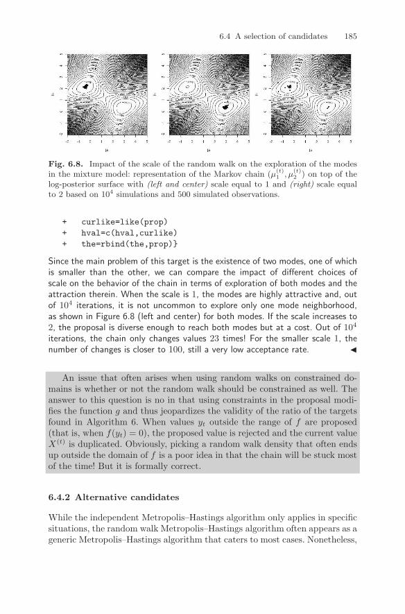
Fig. 6.8. Impact of the scale of the random walk on the exploration of the modesin the mixture model: representation of the Markov chain (µ

(t)1 , µ

(t)2 ) on top of the

log-posterior surface with (left and center) scale equal to 1 and (right) scale equalto 2 based on 104 simulations and 500 simulated observations.

+ curlike=like(prop)+ hval=c(hval,curlike)+ the=rbind(the,prop)}

Since the main problem of this target is the existence of two modes, one of whichis smaller than the other, we can compare the impact of different choices ofscale on the behavior of the chain in terms of exploration of both modes and theattraction therein. When the scale is 1, the modes are highly attractive and, outof 104 iterations, it is not uncommon to explore only one mode neighborhood,as shown in Figure 6.8 (left and center) for both modes. If the scale increases to2, the proposal is diverse enough to reach both modes but at a cost. Out of 104

iterations, the chain only changes values 23 times! For the smaller scale 1, thenumber of changes is closer to 100, still a very low acceptance rate. J

An issue that often arises when using random walks on constrained do-mains is whether or not the random walk should be constrained as well. Theanswer to this question is no in that using constraints in the proposal modi-fies the function g and thus jeopardizes the validity of the ratio of the targetsfound in Algorithm 6. When values yt outside the range of f are proposed(that is, when f(yt) = 0), the proposed value is rejected and the current valueX(t) is duplicated. Obviously, picking a random walk density that often endsup outside the domain of f is a poor idea in that the chain will be stuck mostof the time! But it is formally correct.

6.4.2 Alternative candidates

While the independent Metropolis–Hastings algorithm only applies in specificsituations, the random walk Metropolis–Hastings algorithm often appears as ageneric Metropolis–Hastings algorithm that caters to most cases. Nonetheless,


the random walk solution is not necessarily the most efficient choice in that(a) it requires many iterations to overcome difficulties such as low-probabilityregions between modal regions of f and (b) because of its symmetric features,it spends roughly half the simulation time revisiting regions it has alreadyexplored. There exist alternatives that bypass the perfect symmetry in therandom walk proposal to gain in efficiency, although they are not always easyto implement (see, for example, Robert and Casella, 2004).

One of those alternatives is the Langevin algorithm of Roberts and Rosen-thal (1998) that tries to favor moves toward higher values of the target f byincluding a gradient in the proposal,

Yt = X(t) +σ2

2∇ log f(X(t)) + σεt , εt ∼ g(ε) ,

the parameter σ being the scale factor of the proposal. When Yt is constructedthis way, the Metropolis–Hastings acceptance probability is equal to

ρ(x, y) = min{f(y)f(x)

g [(x− y)/σ − σ∇ log f(y)/2]g [(y − x)/σ − σ∇ log f(x)/2]

, 1}.

While this scheme may remind you of the stochastic gradient techniquesof Section 5.3.2, it differs from those for two reasons. One is that the scale σis fixed in the Langevin algorithm, as opposed to decreasing in the stochasticgradient method. Another is that the proposed move to Yt is not necessarilyaccepted for the Langevin algorithm, ensuring the stationarity of f for theresulting chain.

Example 6.6. Based on the same probit model of the now well-known Pima.trdataset as in Example 3.10, we can use the likelihood function like alreadydefined on page 85 and compute the gradient in closed form as

grad=function(a,b){don=pnorm(q=a+outer(X=b,Y=da[,2],FUN="*"))x1=sum((dnorm(x=a+outer(X=b,Y=da[,2],FUN="*"))/don)*da[,1]-

(dnorm(x=-a-outer(X=b,Y=da[,2],FUN="*"))/(1-don))*(1-da[,1]))

x2=sum(da[,2]*((dnorm(x=a+outer(X=b,Y=da[,2],FUN="*"))/don)*da[,1]-(dnorm(x=-a-outer(X=b,Y=da[,2],FUN="*"))/

(1-don))*(1-da[,1])))return(c(x1,x2))}

When implementing the basic iteration of the Langevin algorithm

> prop=curmean+scale*rnorm(2)> propmean=prop+0.5*scale^2*grad(prop[1],prop[2])


> if (log(runif(1))>like(prop[1],prop[2])-likecur-+ sum(dnorm(prop,mean=curmean,sd=scale,lo=T))++ sum(dnorm(the[t-1,],mean=propmean,sd=scale,lo=T))){+ prop=the[t-1,];propmean=curmean}

we need to select scale small enough because otherwise grad(prop) returns NaNgiven that pnorm(q=a+outer(X=b,Y=da[,2],FUN="*")) is then either 1 or 0.With a scale equal to 0.01, the chain correctly explores the posterior distribution,as shown in Figure 6.9, even though it moves very slowly. J

Fig. 6.9. Repartition of the Langevin sample corresponding to the probit posteriordefined in Example 3.10 based on 20 observations from Pima.tr and 5×104 iterations.

The modification of the random walk proposal may, however, further hin-der the mobility of the Markov chain by reinforcing the polarization aroundlocal modes. For instance, when the target is the posterior distribution of themixture model studied in Example 6.5, the bimodal structure of the targetis a hindrance for the implementation of the Langevin algorithm in that thelocal mode becomes even more attractive.


Example 6.7. (Continuation of Example 6.5) The modification of therandom walk Metropolis–Hastings algorithm is straightforward in that we simplyhave to add the gradient drift in the R code. Defining the gradient function

gradlike=function(mu){deno=.2*dnorm(da-mu[1])+.8*dnorm(da-mu[2])gra=sum(.2*(da-mu[1])*dnorm(da-mu[1])/deno)grb=sum(.8*(da-mu[2])*dnorm(da-mu[2])/deno)return(c(gra,grb))}

the simulation of the Markov chain involves

> prop=curmean+rnorm(2)*scale> meanprop=prop+.5*scale^2*gradlike(prop)> if ((max(-prop)>2)||(max(prop)>5)||(log(runif(1))>like(prop)+ -curlike-sum(dnorm(prop,curmean,lo=T))++ sum(dnorm(the[iter,],meanprop,lo=T)))){+ prop=the[iter,]+ meanprop=curmean+ }> curlike=like(prop)> curmean=meanprop

When running this Langevin alternative on the same dataset as in Example 6.5,the scale needs to be reduced quite a lot for the chain to move. For instance,using scale=.2 was not small enough for this purpose and we had to lowerit to scale=.1 to start seeing high enough acceptance rates. Figure 6.10 isrepresentative of the impact of the starting point on the convergence of the chainsince starting near the wrong mode leads to a sample concentrated on this verymode. The reason for this difficulty is that, with 500 observations, the likelihoodis very peaked and so is the gradient. J

Both examples above show how delicate the tuning of the Langevin al-gorithm can be. This may explain why it is not widely implemented, eventhough it is an easy enough modification of the basic random walk code.

Random walk Metropolis–Hastings algorithms also apply to discrete sup-port targets. While this sounds more like a combinatoric or an image-processing setting, since most statistical problems involve continuous parame-ter spaces, an exception is the case of model choice (see, for example, Robert,2001, Chapter 7), where the index of the model to be selected is the “param-eter” of interest.

Example 6.8. Given an ordinary linear regression with n observations,

y|β, σ2, X ∼ Nn(Xβ, σ2In) ,

where X is a (n, p) matrix, the likelihood is


Fig. 6.10. Exploration of the modes in the mixture model by a Langevin algorithm:representation of two Markov chains (µ

(t)1 , µ

(t)2 ) on top of the log-posterior surface

with a scale equal to .1 based on 104 simulations and a simulated dataset of 500observations.


`(β, σ2|y, X

)=(2πσ2

)−n/2exp

[− 1

2σ2(y −Xβ)T(y −Xβ)

]and, under the so-called g-prior of Zellner (1986),

β|σ2, X ∼ Nk+1(β̃, nσ2(XTX)−1) and π(σ2|X) ∝ σ−2

(where the constant g is chosen equal to n), the marginal distribution of y is amultivariate t distribution,

m(y|X) = (n+ 1)−(k+1)/2π−n/2Γ (n/2)[yTy − n

n+ 1yTX(XTX)−1XTy

− 1n+ 1

β̃TXTXβ̃

]−n/2.

As an illustration, we consider the swiss dataset, where the logarithm of thefertility in 47 districts of Switzerland around 1888 is the variable y to be explainedby some socioeconomic indicators,

> y=log(as.vector(swiss[,1]))> X=as.matrix(swiss[,2:6])

The covariate matrix X involves five explanatory variables

> names(swiss)[1] "Fertility" "Agriculture" "Examination" "Education"[5] "Catholic" "Infant.Mortality"

(that are explained by ?swiss) and we want to compare the 25 models corre-sponding to all possible subsets of covariates. (In this toy example, the numberof models is small enough to allow for the computation of all marginals andtherefore the true probabilities of all models under comparison.) Following Marinand Robert (2007), we index all models by vectors γ of binary indicators whereγi = 0 indicates that the corresponding column of X is used in the regression.(Note that, adopting Marin and Robert’s, 2007, convention, we always includethe intercept in a model.) Using the fast inverse matrix function

inv=function(X){EV=eigen(X)EV$vector%*%diag(1/EV$values)%*%t(EV$vector)}

we then compute the log marginal density corresponding to the model γ, nowdenoted as m(y|X, γ), as

lpostw=function(gam,y,X,beta){n=length(y)qgam=sum(gam)Xt1=cbind(rep(1,n),X[,which(gam==1)])


if (qgam!=0) P1=Xt1%*%inv(t(Xt1)%*%Xt1)%*%t(Xt1) else{P1=matrix(0,n,n)}-(qgam+1)/2*log(n+1)-n/2*log(t(y)%*%y-n/(n+1)*t(y)%*%P1%*%y-1/(n+1)*t(beta)%*%t(cbind(rep(1,n),X))%*%P1%*%cbind(rep(1,n),X)%*%beta)

}

The exploration of the space of models can result from a Metropolis–Hastings al-gorithm that moves around models by changing one model indicator at a time;that is, given the current indicator vector γ(t), the Metropolis–Hastings proposal

picks one of the p coordinates, say i, and chooses between keeping γ(t)i and

switching to 1− γ(t)i with probabilities proportional to the associated marginals.

The Metropolis–Hastings acceptance probability of the proposed model γ? is thenequal to

min{m(y|X, γ?)m(y|X, γ(t))

m(y|X, γ(t))m(y|X, γ?)

, 1}

= 1

since the normalising constants cancel. This means that we do not have to considerrejecting the proposed model γ? because it is always accepted at the Metropolis–Hastings step! Running the R function

gocho=function(niter,y,X){lga=dim(X)[2]beta=lm(y∼X)$coeffgamma=matrix(0,nrow=niter,ncol=lga)gamma[1,]=sample(c(0,1),lga,rep=T)for (t in 1:(niter-1)){j=sample(1:lga,1)gam0=gam1=gamma[t,];gam1[j]=1-gam0[j]pr=lpostw(gam0,y,X,beta)pr=c(pr,lpostw(gam1,y,X,beta))pr=exp(pr-max(pr))gamma[t+1,]=gam0if (sample(c(0,1),1,prob=pr))

gamma[t+1,]=gam1}gamma}

then produces a sample (approximately) distributed from the posterior distributionon the set of indicators; that is, on the collection of possible submodels. Basedon the outcome

> out=gocho(10^5,y,X)

the most likely model corresponds to the exclusion of the Agriculture variable(that is, γ = (1, 0, 1, 1, 1)), with estimated probability 0.4995, while the trueprobability is 0.4997. (This model is also the one indicated by lm(y∼X).) Similarly,


the second most likely model is γ = (0, 0, 1, 1, 1), with an estimated probabilityof 0.237 versus a true probability of 0.234. The probability that each variable isincluded within the model is also provided by

> apply(out,2,mean)[1] 0.66592 0.17978 0.99993 0.91664 0.94499

which, again, indicates that the last three variables of swiss are the most signif-icant in this analysis. J

The fact that the acceptance probability is always equal to 1 in Example6.8 is due to the use of the true target probability on a subset of the possiblevalues of the model indicator.

Exercise 6.5 Starting from the prior distribution

β|σ2, X ∼ Nk+1(β̃, nσ2(XTX)−1) :

a. Show thatXβ|σ2, X ∼ Nn(Xβ̃, nσ2X(XTX)−1XT)

and thaty|σ2, X ∼ Nn(Xβ̃, σ2(In + nX(XTX)−1XT)) .

b. Show that integrating in σ2 with π(σ2) = 1/σ2 yields the marginal distribu-tion of y above.

c. Compute the value of the marginal density of y for the swiss dataset.

6.5 Acceptance rates

There are infinite choices for the candidate distribution q in a Metropolis–Hastings algorithm, and here we discuss the possibility of achieving an “op-timal” choice. Most obviously, this is not a well-defined concept in that the“optimal” choice of q is to take q = f , the target distribution, when reason-ing in terms of speed of convergence. This is obviously a formal result thathas no relevance in practice! Instead, we need to adopt a practical criterionthat allows the comparison of proposal kernels in situations where (almost)nothing is known about f . One such criterion is the acceptance rate of thecorresponding Metropolis–Hastings algorithm since it can be easily computedwhen running this algorithm via the empirical frequency of acceptance. Incontrast to Chapter 2, where the calibration of an Accept–Reject algorithmwas based on the maximum acceptance rate, merely optimizing the accep-tance rate will not necessarily result in the best algorithm in terms of mixingand convergence.

6.5 Acceptance rates 193

Fig. 6.11. Cumulative mean plot (left) from a Metropolis–Hastings algorithmused to generate a N (0, 1) random variable from a double-exponential proposaldistribution L(1) (lighter) and L(3) (black). The center and left panels show theautocovariance for the L(1) and L(3) proposals, respectively.

Example 6.9. In an Accept–Reject algorithm generating a N (0, 1) sample froma double-exponential distribution L(α) with density g(x|α) = (α/2) exp(−α|x|),the choice α = 1 optimizes the acceptance rate (Exercise 2.19). We can use thisdistribution as an independent candidate q in a Metropolis–Hastings algorithm.Figure 6.11 compares the behavior of this L(1) candidate along with an L(3)distribution, which, for this simulation, produces an inferior outcome in the sensethat it has larger autocovariances and, as a result of this, slower convergence.Obviously, a deeper analysis would be necessary to validate this statement, butour point here is that the acceptance rate (estimated) for α = 1 is twice as large,0.83, as the acceptance rate (estimated) for α = 3, 0.47. J

While independent Metropolis–Hastings algorithms can indeed be opti-mized or at least compared through their acceptance rate, because this reducesthe number of replicas in the chain {X(t)} and thus the correlation level inthe chain, this is not true for other types of Metropolis–Hastings algorithms,first and foremost the random walk version.

Exercise 6.6 The inverse Gaussian distribution has the density

f(z|θ1, θ2) ∝ z−3/2 exp{−θ1z −

θ2z

+ 2√θ1θ2 + log

√2θ2

}on R+ (θ1 > 0, θ2 > 0).

a. A candidate for a Metropolis–Hastings algorithm targeting f is the G(α, β)distribution. Show that


f(x)g(x)

∝ x−α−1/2 exp{

(β − θ1)x− θ2x

}is maximized in x at

x∗β =(α+ 1/2)−

√(α+ 1/2)2 + 4θ2(θ1 − β)2(β − θ1)

.

b. After maximizing in x, the goal would be to minimize the bound on f/g over(α, β) for fixed (θ1, θ2). This is impossible analytically, but for chosen valuesof (θ1, θ2) we can plot this function of (α, β). Do so using for instance persp.Do any patterns emerge?

c. The mean of the inverse Gaussian distribution is√θ2/θ1, so taking α =

β√θ2/θ1 will make the means of the candidate and target coincide. For

θ1 = θ2, match means and find an “optimal” candidate in terms of theacceptance rate.

The random walk version of the Metropolis–Hastings algorithm, intro-duced in Section 6.4.1, does indeed require a different approach to acceptancerates, given the dependence of the candidate distribution on the current stateof the chain. In fact, as already seen in Example 6.4, a high acceptance ratedoes not necessarily indicate that the algorithm is behaving satisfactorily sinceit may instead correspond to the fact that the chain is moving too slowly onthe surface of f . When x(t) and yt are close, in the sense that f(x(t)) andf(yt) are approximately equal, the random walk Metropolis–Hastings algo-rithm leads to the acceptance of yt with probability

min(f(yt)f(x(t))

, 1)' 1.

A high acceptance rate may therefore signal a poor convergence pattern asthe moves on the support of f are more limited. Obviously, this is not al-ways the case. For instance, when f is nearly flat, high acceptance rates arenot indicative of any wrong behavior! But, unless f is completely flat (thatis, it corresponds to a uniform target), there are parts of the domain to beexplored where f takes smaller values and hence where the acceptance prob-abilities should be small. A high acceptance rate then indicates that thoseparts of the domain are not often (or not at all!) explored by the Metropolis–Hastings algorithm.

In contrast, if the average acceptance rate is low, the successive values off(yt) often are small when compared with f(x(t)), which corresponds to thescenario where the random walk moves quickly on the surface of f since itoften reaches the “borders” of the support of f (or at least when the randomwalk explores regions with low probability under f). Again, a low acceptancerate does not mean that the chain explores the entire support of f . Even with

6.6 Additional exercises 195

a small acceptance rate, it may miss an important but isolated mode of f .Nonetheless, a low acceptance rate is less of an issue, except from the com-puting time point of view, because it explicitly indicates that a larger numberof simulations are necessary. Using the effective sample size as a convergenceindicator (see Section 8.4.3) would clearly signal this requirement.

Example 6.10. (Continuation of Example 6.4) The three random walkMetropolis–Hastings algorithms of Figure 6.7 have acceptance rates equal to

[1] 0.9832[1] 0.7952[1] 0.1512

respectively. Looking at the histogram fit, we see that the medium acceptancerate does better but that the lowest acceptance rate still fares better than thehighest one. J

The question is then to decide on a golden acceptance rate against which tocalibrate random walk Metropolis–Hastings algorithms in order to avoid “toohigh” as well as “too low” acceptance rates. Roberts et al. (1997) recommendthe use of instrumental distributions with acceptance rates close to 1/4 formodels of high dimension and equal to 1/2 for the models of dimension 1 or 2.(This is the rule adopted in the adaptive amcmc package described in Section8.5.2.) While this rule is not universal (in the sense that it was primarilydesigned for a Gaussian environment), we advocate it as a default calibrationgoal whenever it can be achieved (which is not always the case). For instance,if we consider the Metropolis–Hastings algorithm in Example 6.8, there is noacceptance rate since the acceptance probability is always equal to 1. However,since the proposal includes the current value in its support, the chain {γ(t)}has identical values in a row and thus an implicit acceptance (or renewal) rate.It is equal to 0.1805, much below the 0.25 goal, and the algorithm cannot beeasily modified (for instance, by looking at more alternative moves around thecurrent model) to reach this token acceptance rate.

6.6 Additional exercises

Exercise 6.7 Referring to Example 2.7, consider a Be(2.7, 6.3) target density.

a. Generate Metropolis–Hastings samples from this density using a range of indepen-dent beta candidates from a Be(1, 1) to a beta distribution with small variance.(Note: Recall that the variance is ab/(a+ b)2(a+ b+ 1).) Compare the acceptancerates of the algorithms.

b. Suppose that we want to generate a truncated beta Be(2.7, 6.3) restricted tothe interval (c, d) with c, d ∈ (0, 1). Compare the performance of a Metropolis–Hastings algorithm based on a Be(2, 6) proposal with one based on a U(c, d) pro-posal. Take c = .1, .25 and d = .9, .75.


Exercise 6.8 While q is a Markov kernel used in Algorithm 4, it is not the Markovkernel K of the algorithm.

1. Show that the probability that X(t+1) = x(t) is

ρ(x(t)) =

Z n1− ρ(x(t), y)

oq(y|x(t)) dy .

2. Deduce that the kernel K can be written as

K(x(t), y) = ρ(x(t), y)q(y|x(t)) + ρ(x(t))δx(t)(y) .

3. Show that Algorithm 4 satisfies the detailed balance condition (6.3).

Exercise 6.9 Calculate the mean of a gamma G(4.3, 6.2) random variable using

a. Accept–Reject with a gamma G(4, 7) candidate;b. Metropolis–Hastings with a gamma G(4, 7) candidate;c. Metropolis–Hastings with a gamma G(5, 6) candidate.

In each case, monitor the convergence across iterations.

Exercise 6.10 Student’s t density with ν degrees of freedom, Tν , is given by

f(x|ν) =Γ`ν+1

2

´Γ`ν2

´ 1√νπ

`1 + x2/ν

´−(ν+1)/2.

Calculate the mean of a t distribution with ν = 4 degrees of freedom using a Metropolis–Hastings algorithm with candidate density

a. N (0, 1);b. t with ν = 2 degrees of freedom.

In each case monitor the convergence across iterations.

Exercise 6.11 Referring to Example 6.3:

1. Use the candidate given in this example to generate a sample (a(i), b(i), c(i)), i =1, . . . , 500 with a Metropolis–Hastings algorithm. The data is from the datasetcars.

2. Monitor convergence and check autocorrelations for each parameter across itera-tions.

3. Make histograms of the posterior distributions of the coefficient estimates, andprovide 95% confidence intervals.

Exercise 6.12 Still in connection with Example 6.3, show that the posterior distribu-tion on (a, b, c, σ−2) is a standard distribution made of a trivariate normal on (a, b, c)conditional on σ and the data and a gamma distribution on σ−2 given the data. (Hint:See Robert, 2001, or Marin and Robert, 2007, for details.)

Exercise 6.13 In 1986, the space shuttle Challenger exploded during takeoff, killingthe seven astronauts aboard. The explosion was the result of an O-ring failure, a splittingof a ring of rubber that seals the parts of the ship together. The accident was believed tohave been caused by the unusually cold weather (31o F or 0o C) at the time of launch,as there is reason to believe that the O-ring failure probabilities increase as temperaturedecreases. Data on previous space shuttle launches and O-ring failures is given in thedataset challenger provided with the mcsm package. The first column corresponds tothe failure indicators yi and the second column to the corresponding temperature xi(1 ≤ i ≤ 24).

6.6 Additional exercises 197

1. Fit this dataset with a logistic regression, where

P (Yi = 1|xi) = p(xi) = exp(α+ βxi)‹

1 + exp(α+ βxi) ,

using R glm function, as illustrated on page 21. Deduce the MLEs for α and β,along with standard errors.

2. Set up a Metropolis–Hastings algorithm with the likelihood as target using an expo-nential candidate for α and a Laplace (double-exponential) candidate for β. (Hint:Choose the parameters of the candidates based on the MLEs derived in a.)

3. Generate 5000 iterations of the Markov chain and construct a picture similar toFigure 6.6 to evaluate the variability of p(x) minus the observation dots.

4. Derive from this sample an estimate of the probability of failure at 60o, 50o, and40o F along with a standard error.


a. Reproduce the graphs in Figure 6.7 for difference values of δ. Explore both smalland large δ’s. Can you find an optimal choice in terms of autocovariance?

b. The random walk candidate can be based on other distributions. Consider generatinga N (0, 1) distribution using a random walk with a (i) Cauchy candidate, and a (ii)Laplace candidate. Construct these Metropolis–Hastings algorithms and comparethem with each other and with the Metropolis–Hastings random walk with a uniformcandidate.

c. For each of these three random walk candidates, examine whether or not the ac-ceptance rate can be brought close to 0.25 for the proper choice of parameters.


a. Write a Metropolis–Hastings algorithm to produce Figure 6.11. Note that n L(a)random variables can be generated at once with the R command

> ifelse(runif(n)>0.5, 1, -1) * rexp(n)/a

b. What is the acceptance rate for the Metropolis–Hastings algorithm with candidateL(3)? Plot the curve of the acceptance rates for L(α) candidates when α variesbetween 1 and 10. Comment.

c. Plot the curve of the acceptance rates for candidates L(0, ω) when ω varies between.01 and 10. Compare it with those of the L(α) candidates.

d. Plot the curve of the acceptance rates when the proposal is based on a random walk,Y = X(t) + ε, where ε ∼ L(α). Once again, compare it with the earlier proposals.

Exercise 6.16 In connection with Example 6.8, compare the current implementationwith an alternative where more values are considered at once according to the R code

> progam=matrix(gama[i,],ncol=lga,nrow=lga,byrow=T)

> probam=rep(0,lga)

> for (j in 1:lga){

+ progam[j,j]=1-gama[i,j]

+ probam[j]=lpostw(progam[j,],y,X,betatilde)}

> probam=exp(probam)

> sumam=sum(probam)

> probam=probam/sumam

> select=progam[sample(1:lga,1,prob=probam),]

a. Show that the acceptance probability is different from 1 and involves sumam.b. Study the speed of convergence of the evaluation of the posterior probability of the

most likely model in comparison with the implementation on page 191.

http://www.springer.com/978-1-4419-1575-7

6 metropolis{hastings algorithms - .net framework

Documents