6. rectification 2 hours - uacg.bg · ... master course photogrammetry 2003 b. marinov . lecture 6...

Lecture 6 - 1 - 11/2/2003 ____________________________________________________________________________________

Concept Hell/Pfeiffer February 2003 ___________________________________________________________________________________

6. Rectification 2 hours Aim: Principles for rectification Theory: Indirect rectification in digital image processing Methods of rectification and integration in programs ___________________________________________________________________________________ 6.1. The deformations of metric photograph A line map is unsatisfactory for some regions (undeveloped areas). Photo-map is a map that

shows the content of the aerial photographs and is better solution. Photo maps are significantly

less expensive and quicker for producing in comparison to conventional topographic line maps.

The deformations of images, including photographs are described in differential geometry by

means of the Tissot indicatrix. This theory is developed for analytical surfaces. Ground surface is

represented in photogrammetry by digitizing a large set of individual points on the surface

Another method is based on the closely spaced discrete points, defined by their XYZ-coordinates.

The deformation between photograph and terrain are described by co-linearity equations

11 0 21 0 31 0

13 0 23 0 33 0

12 0 22 0 32 0

13 0 23 0 33 0

.( ) .( ) .( ).

.( ) .( ) .( ).( ) .( ) .( )..( ) .( ) .( )

i i ip

i i i

i i ip

i i i

r X X r Y Y r Z Zx x cr X X r Y Y r Z Zr X X r Y Y r Z Zy y cr X X r Y Y r Z Z

− + − + −− = −

− + − + −− + − + −

− = −− + − + −

(6.1)

Geometrically this deformation is presented in the next figure

____________________________________________________________________________________ FH-KA - Master course Photogrammetry 2003 B. Marinov

Lecture 6 - 2 - 11/2/2003 ____________________________________________________________________________________

Figure 6.1. Relations between grids in object and photo

The estimation of deformation can be obtain by the deformation of square grid, shown on the

next figure


Lecture 6 - 3 - 11/2/2003 ____________________________________________________________________________________

1 2

3 4

1’ 2’

3’ 4’

ξ

η Y

X

Figure 6.2. Deformations of square grid

Deformations in length in X and Y directions are given by expressions

12 13 , x yX Yδ δλ λ=∆ ∆

= (6.2)

where 2( ) (ik i k i kδ ξ ξ η η= − + − 2) (6.3)

Deformations of grid and photos due to the projection and terrain are presented in the next figure

Figure 6.3. Deformed grid of aerial photograph

For plane object surface the deformation can be see very clearly in comparison with XY-grid of

the object


Lecture 6 - 4 - 11/2/2003 ____________________________________________________________________________________

ξ

η Y

X

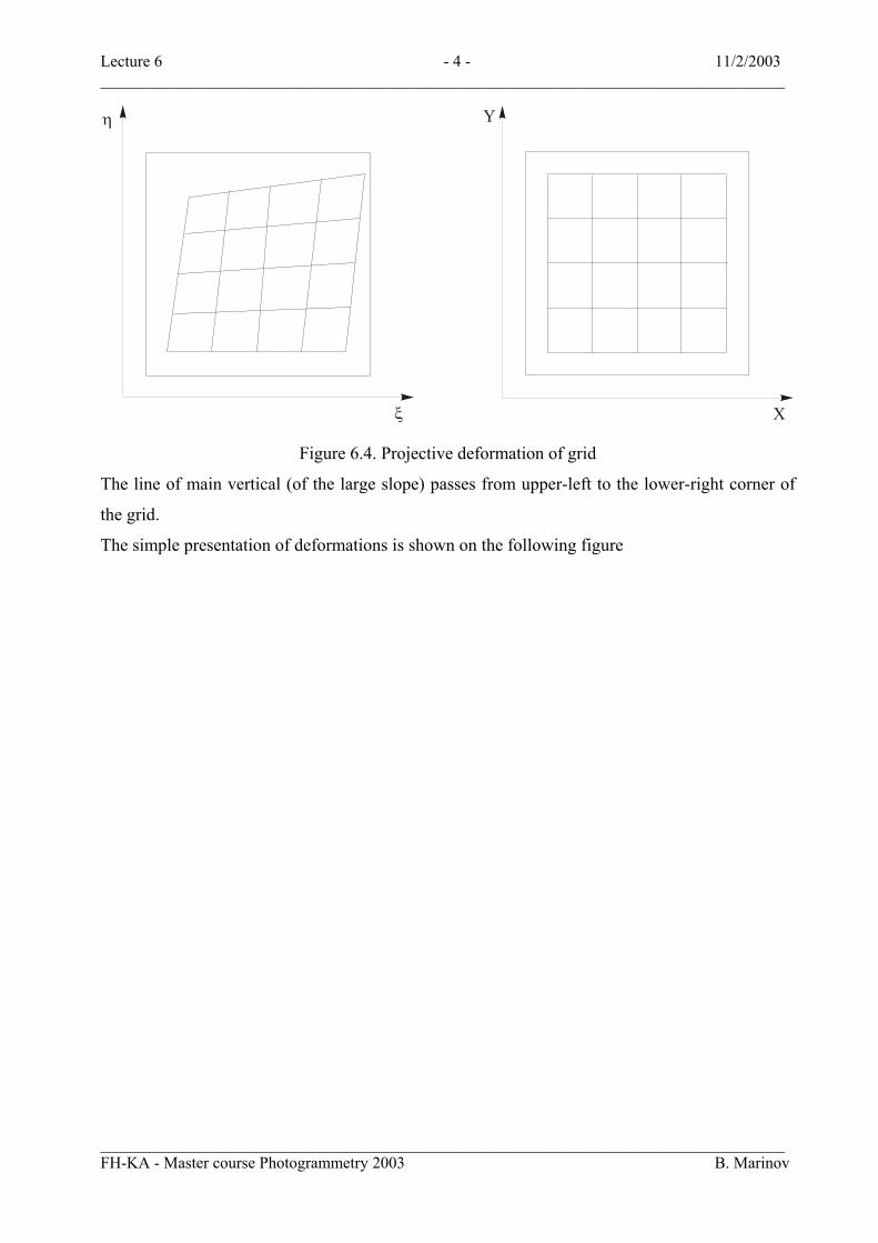
Figure 6.4. Projective deformation of grid

The line of main vertical (of the large slope) passes from upper-left to the lower-right corner of

the grid.

The simple presentation of deformations is shown on the following figure


Lecture 6 - 5 - 11/2/2003 ____________________________________________________________________________________

ντ

τ

0

ρ

ρ

0

a

a 0

A

pn p

N

0 0

n

O

Figure 6.5. Reduction of length in tilted photograph.

The radial displacement of point position with radius ρ for small angles of tilt ν is presented by

expression 2

.vc

ρρ∆ = (6.4)

where 2 2ρ ξ η= + and 2 2ρ ξ η∆ = ∆ + ∆

The increase or reduction of small lengths dρ is obtained by differentiating the previous

expression

( ) 2. . .dc

dρρ ν ρ∆ = (6.5)

The photograph is similar to the orthophoto (without geometrical distortions) if the object plane

and image plane are made parallel. The images that does not lye in this plane are displaced from

there actual position depending on the difference of distance from the projection center (that

means different height for aerial photos).


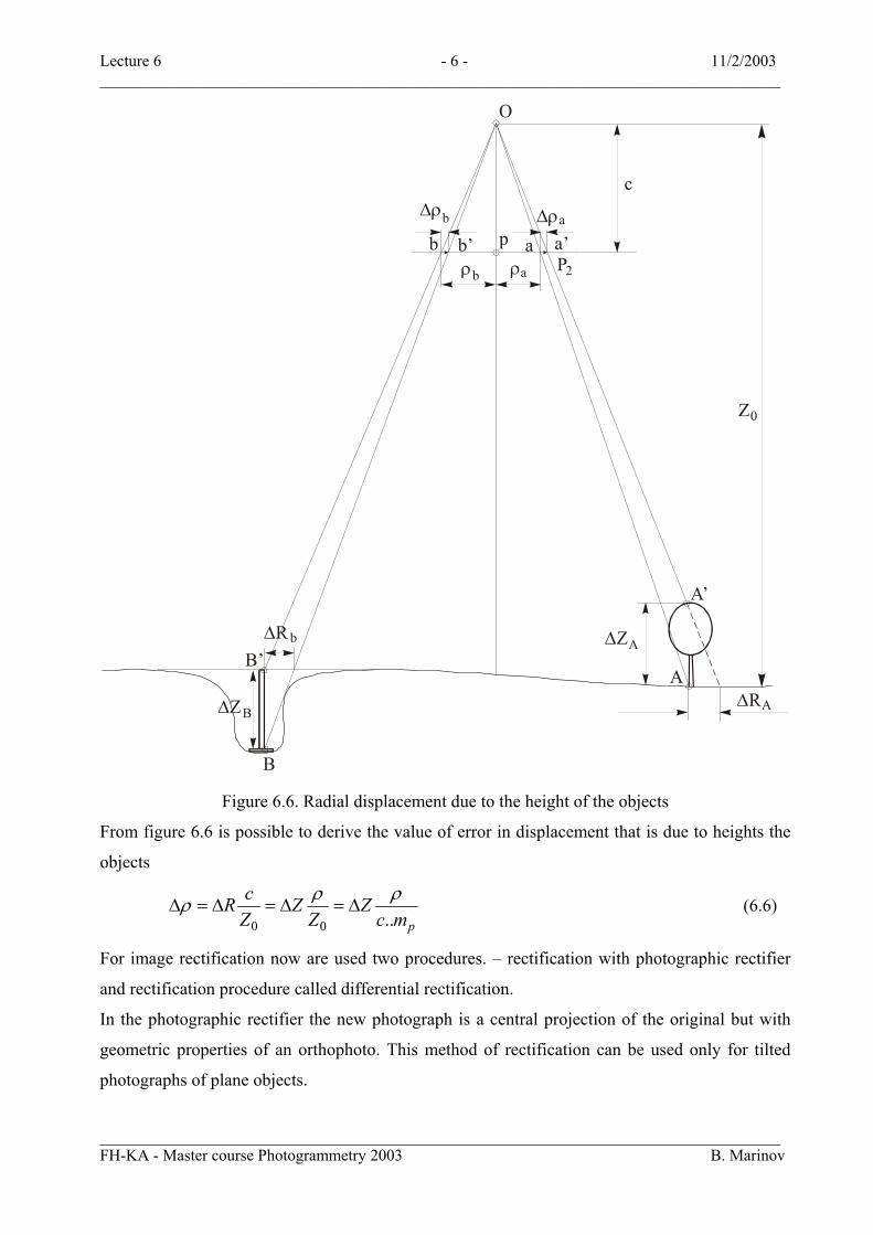
Lecture 6 - 6 - 11/2/2003 ____________________________________________________________________________________

P2

A’

A

B

O

∆R b

B’

∆ρa∆ρb

a’ab b’bρ ρa

p

∆ZA

∆RA∆ZB

Z0

c

Figure 6.6. Radial displacement due to the height of the objects

From figure 6.6 is possible to derive the value of error in displacement that is due to heights the

objects

0 0 .. p

cR Z ZZ Z c m

ρ ρρ∆ = ∆ = ∆ = ∆ (6.6)

For image rectification now are used two procedures. – rectification with photographic rectifier

and rectification procedure called differential rectification.

In the photographic rectifier the new photograph is a central projection of the original but with

geometric properties of an orthophoto. This method of rectification can be used only for tilted

photographs of plane objects.


Lecture 6 - 7 - 11/2/2003 ____________________________________________________________________________________

6.2. Rectification by central perspective transformation There are two possible methods for perspective rectification – with and without establishment of

inner orientation parameters in the rectifier.

6.2.1. Perspective rectification with establishment of inner orientation The inner and outer orientation of original photograph must reestablished for the solution of

rectification task.

Figure 6.7. Rectifier with reestablished inner and outer orientation

The projector has fiducial marks for reestablishements of the inner orientation. Three elements of

outer orientation can be set: z0 of the projector, rotations ω and φ.

00

0

Zzm

= (6.7)

where m0 is the scale factor of the orthophoto ____________________________________________________________________________________ FH-KA - Master course Photogrammetry 2003 B. Marinov

Lecture 6 - 8 - 11/2/2003 ____________________________________________________________________________________

The focal length of the projector lens must be different from the focal length of the original

camera lens. This rectifier requires three control points from which the six elements of outer

orientation can be determined (from them only three are important for rectification).

6.2.2. Perspective rectification with reestablishment of inner orientation. It is necessary to satisfy two optical condition to achieve a sharp projected image over the full

format.

Optical conditions

The plane of the photograph in the rectifier must be tilted relative to the optical axis. This

condition however is not satisfied in metric cameras where the plane of photograph is

perpendicular to the optical axis of the camera.

First optical condition is called Scheimpflug condition, because T.Sheimpflug first developed it.

importance. It says that plane of the photograph IP, the principle plane of the objective He

and the plane of the projection stage PS must intersect in the same straight line S. This is

shown at the figure 6.8.


Lecture 6 - 9 - 11/2/2003 ____________________________________________________________________________________

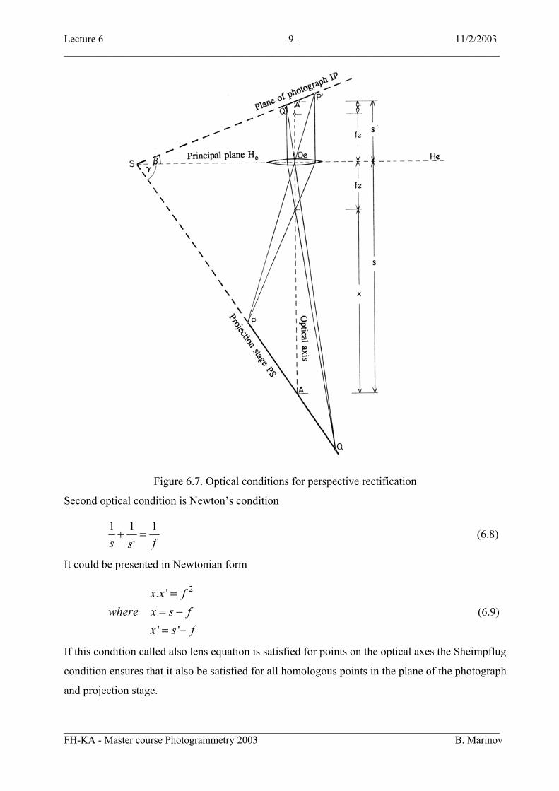
Figure 6.7. Optical conditions for perspective rectification

Second optical condition is Newton’s condition

,1 1 1s fs

+ = (6.8)

It could be presented in Newtonian form

2 . '

' '

x x fwhere x s f

x s f

== −= −

(6.9)

If this condition called also lens equation is satisfied for points on the optical axes the Sheimpflug

condition ensures that it also be satisfied for all homologous points in the plane of the photograph

and projection stage.


Lecture 6 - 10 - 11/2/2003 ____________________________________________________________________________________

The lens equation and Scheimpflug condition are satisfied by mechanical devices, so-called

inversors and by electronic control systems in newer instruments.

Geometric conditions

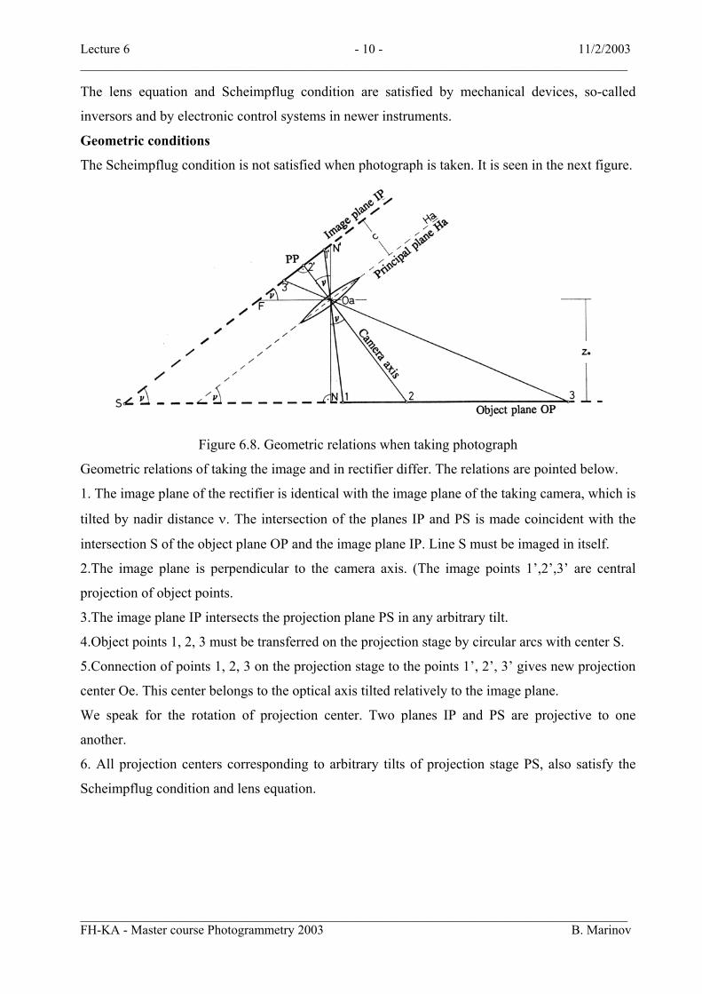
The Scheimpflug condition is not satisfied when photograph is taken. It is seen in the next figure.

Figure 6.8. Geometric relations when taking photograph

Geometric relations of taking the image and in rectifier differ. The relations are pointed below.

1. The image plane of the rectifier is identical with the image plane of the taking camera, which is

tilted by nadir distance ν. The intersection of the planes IP and PS is made coincident with the

intersection S of the object plane OP and the image plane IP. Line S must be imaged in itself.

2.The image plane is perpendicular to the camera axis. (The image points 1’,2’,3’ are central

projection of object points.

3.The image plane IP intersects the projection plane PS in any arbitrary tilt.

4.Object points 1, 2, 3 must be transferred on the projection stage by circular arcs with center S.

5.Connection of points 1, 2, 3 on the projection stage to the points 1’, 2’, 3’ gives new projection

center Oe. This center belongs to the optical axis tilted relatively to the image plane.

We speak for the rotation of projection center. Two planes IP and PS are projective to one

another.

6. All projection centers corresponding to arbitrary tilts of projection stage PS, also satisfy the

Scheimpflug condition and lens equation.


Lecture 6 - 11 - 11/2/2003 ____________________________________________________________________________________

Figure 6.9.Rectification with not congruent bundle of rays

The relations between geometrical characteristics are shown in Appendix 1.

This rectifiers are with bundle of rays that is not congruent to that of the original photograph

Rectification with known instrument settings

When we calculate the outer orientation parameters of photo we obtain coordinates of the

projection center X0, Y0, Z0 and three rotation angles ω, φ, κ. From this parameters we must

derive the direction α, the nadir distance ϖ and swing κ.


Lecture 6 - 12 - 11/2/2003 ____________________________________________________________________________________

Figure 6.10. Definition of rectification angles

We construct new spatial rotation matrix

aR R R Rανκ ν κ= (6.10)

After expression in analytical form is possible to obtain angle elements from the coefficients of

rotation matrix

13 1333

23 32tan cos tanr rr

r rα ν= =

−κ = (6.11)

It is possible to make rectification with control points and with knowledge of the inner

orientation. For such orientation sufface three control points. However usually four control

points are used. The additional point is for check of the orientation process.

Two step procedure is used.

1. Change the projection distance

2.Tilt of projection stage about two axis (for some rectifiers only one tilt and rotation are given).

In the second case orientation procedure is more complicated.

There is possible to arrange the orientation procedure with control points, but without knowledge

of the inner orientation.

The construction of rectifiers allow two group of possibilities:

1. Group


Lecture 6 - 13 - 11/2/2003 ____________________________________________________________________________________

• Tilts of the projection stage in two directions

• Displacement of the photograph in two directions

2. Group

• Tilt of the projection stage in one direction

• Displacement of the photograph in two directions and rotation of the

photograph.

6.2.3. Errors of perspective rectification Errors of perspective rectification depend on two types of sources. The first one is the error in

establishing the settings in the rectifier that are computed or derived from control points.

The second source of error is due to the diversity of terrain surface from assumed reference plane

for which the rectification is processed.. The errors accordingly to the errors of object heights

may be presented for small angles by equation. The derivation of errors is shown in Appendix 2

For error in the orthophoto plane we obtain the equation

. p

rr Zc m

∆ = ∆ (6.12)

The error are in radial direction from the nadir point of orthophoto. As a conclusion it must be

pointed that area of application of perspective rectification is limited to plane areas with

small diversity of height. The maximum allowed different in height from assumed plane can be

calculated by defining the permissible error (usually 1mm) at the corners of orthophoto by

solving the above equation.

. . pr c mZ

r∆

∆ = (6.13)

where ∆Z is on the terrain, and r is the displacement in orthophoto.


Lecture 6 - 14 - 11/2/2003 ____________________________________________________________________________________

A’

A

B

O

∆R b

B’

∆ρ

a

∆ρ

b

b a

∆ZA

∆RA∆ZB

Z0

∆r∆r

c

ν

np

r r

z =0 m0

Z0

N’

Z0

Figure 6.13. Radial image displacements of points outside the reference plane

The same is influence in the accuracy of the rectified photographs of buildings facades for

elements in front of or behind the plane of the facade.


Lecture 6 - 15 - 11/2/2003 ____________________________________________________________________________________

6.3. Rectifiers 6.3.1. Classification of rectifiers Rectifiers with congruent bundle of rays are not produced because of the lack of sharpness in the

projected image. More over they need different objectives depending of required enlargement

ratio that is practically inconvenient.

There exist some photographic enlargers working with small angles of tilt.

6.3.2. Examples of optical-mechanical rectifiers Rectifiers with rigorously satisfied geometric and optical conditions are produced by firms Zeiss

Jena, Leica Heerbrugg and Zeiss Oberkochen.

Wild E4 has enlargement ratios 0.8-7.0x. Projection stage can be tilted about two perpendicular

axes up to ±15gon. Picture carrier can be displaced in two perpendicular directions up to ±4cm.

The focal length of the objective is 15cm.

The SEG6 Rectifier of Zeiss Oberkochen has approximately the same ranges as Wild E4.

The Rectimat C of Zeiss Jena was equipped with objective 15cm for enlargement ratios 0.85 to

8.0x and with objective 7cm for enlargement ratios 3.0 to 18.0x. These rectifiers can operate with

preset elements of outer orientation.

Figure 6.11. Rectifier ZEG 6

Accuracy of perspective transformation depends on the height error of terrain or the objects

6.4. Digital rectification Th main principal of digital transformation is similar to the general principal of image restoration. ____________________________________________________________________________________ FH-KA - Master course Photogrammetry 2003 B. Marinov

Lecture 6 - 16 - 11/2/2003 ____________________________________________________________________________________

F (i,j) F (i,j) F (i,j)g (k,l)f (k,l)B

I O RR

Figure 6.12. Main scheme for image restoration

The possible sources for geometrical deformation are following:

But in digital rectification the object of restoration are not the radiometric properties but the

geometric properties of the images.

1. Projective transformations

2. Influence of the height of the objects

3. Lens distortions

4. Earth curvature

5. Map projection

Neverthless of source of geometrical deformation main goal of digital rectification is to reverse

the pixel position in this place, that it must have in the undisturb image of the corresponding

scale.

If we have some source of geometric distortion that is described by formulas

),(),(

,

,

IIyBo

IIxBo

jifyjifx

=

= (6.14)

Our goal is to find such reverse transformation

),(),(

,

,

OOyRR

OOxRR

jigyjigx

=

= (6.15)

In the case when the method of nearest neighbour is used the transformations take the form

]5.0),([]5.0),([

,

,

+=

+=

OOyRR

OOxRR

jigEntijigEntj

(6.16)

By reverse solution we can reach to the output coordinates (without corrections). Comparing the

values for this condition for perfect restoration

]5.0),([]5.0),([

]5.0),([]5.0),([

,1,

,1,

+=+=

+=+=

−

−

RRyIRRyRO

RRxIRRxRO

jigEntjigEnti

jigEntjigEntj (6.17)

These are conditions for geometrical restoration

),(),(

),(),(

,1,

,1,

xygxyg

xygxyg

yIyR

xIxR

=

=−

−

(6.18)


Lecture 6 - 17 - 11/2/2003 ____________________________________________________________________________________

There are possible two schemes for digital rectification

- direct method or forward transformation;

- indirect method or reverse transformation.

In direct method the corrected coordinates of input image are calculated. Every pixel obtain its

real value coordinates in the matrix of restored image. It is possible to interpolate this value to

calculate the grey values in raster matrix. Thi smethod is shown graphically on the next figure.

g (k,l)R

m

n

o

o r

Figure 6.13. Direct transformation

Direct transformation method requires more memory because at the intermidate stage it is

necessary to keep not only the greg value but also the coordinates of transformed pixel. The

procedure for finding from which transformed pixel to calculate the interpolated values is

relatively complex.

In the indirect method is used calculation from the pixel coordinates of transformed image. For

this purposes the reverse formula is necessary to be applied. The graphic presentation of this

method is shown on the next figure


Lecture 6 - 18 - 11/2/2003 ____________________________________________________________________________________

g (k,l)R

m

n

o

o r

-1

Figure 6.14. Indirect method

The calculated values in the input image are not integer. To calculate the grey value at the desired

point it is necessary to use some method of grey value interpolation.

There are used defferent methods:

- nearest neighbour; (square interpolation)

-bilinear interpolation;

- triangle;

-bell-shape curve;

-Gauss curve;

- sinc function (sinx/x) for different sizes of interpolation window.

The Graphical presentation and formulas for interpolation methods are shown in the Appendix 3.

Appendixes Appendix 1 From the figure 6.9 can be derived several relations

Tilt of the photograph β:

0

0.sin sineZ fSF

m ν β= = (6.19)

0

0

.sin .sinef mZ

β ν= (6.20)

m0 scale number of orthophoto.

Tilt of the stage γ:


Lecture 6 - 19 - 11/2/2003 ____________________________________________________________________________________

sin sine

a ec fFO FOν γ

= = = (6.21)

sin .sinefc

γ ν= (6.22)

Image distance s’ - ' 'es O A=

' .cos .ees f FO tanγ β= + (6.23)

Substituting the value of eFO we find

tan' . 1tanes f β

γ

= +

(6.24)

Projection distance s - es O A=

Substituting s’ in lens equation we obtain

tan. 1tanes f γ

β

= +

(6.25)

Enlargement ratio (along the optical axis) – for straight lines in image and object perpendicular

to the optical axis

tan' tansvs

γβ

= = (6.26)

Displacement e of the principal point p from optical axis AA’.

.cot' .cotcosefe FP FA c γν

β= − = − (6.27)

Substituting the value of sinγ

2 2 2.sin cotsin cos

ee

f ce

γf γ

γ β−

= − (6.28)

Appendix 2 .. The errors accordingly to the errors of object heights may be presented for small angles by

equation.

0 0. . rr v Z v Z

Z Zρρ∆ = ∆ = ∆ = ∆ (6.29)

The value of Z0 depends on photo scale and photo scale.

0 . pZ c m= (6.30)


Lecture 6 - 20 - 11/2/2003 ____________________________________________________________________________________

For error in the orthophoto plane we obtain the equation

. p

rr Zc m

∆ = ∆ (6.31)

The error are in radial direction from the nadir point of orthophoto.

Appendix 3 The mathematical formulation of interpolation

Presentation of restoration function

( , ) ( , ) ( , )J I

R Ij J i I

F x y F j x i y R x j x y i y=− =−

= −∑ ∑ −∆ ∆ ∆ ∆

−

(6.32)

The restoration process is described in spatial area by relation

( , ) ( , ).[ ( , ) ( , )]J I

D I Ij J i I

E x y F j x i y R x j x y i y R x j x y i y=− =−

= − − − −∑ ∑ ∆ ∆ ∆ ∆ ∆ ∆ (6.33)

The specral presentation of interpolation is obtained by Furier transformation

24( , ) ( , ) ( ,.

)R x y x y I x xs y ysj i

F R F jx y

∞ ∞

=−∞ =−∞

πω ω = ω ω ω − ω ω − ω∑ ∑

∆ ∆i (6.34)

This presentation allows easier to estimate the errors of interpolation

The presentation of different types of iterpolation function is shown in the next table


Lecture 6 - 21 - 11/2/2003 ____________________________________________________________________________________

Function Graphic presentation Definition in spatial area Spectral Presentation sinc

y

sin(2 // )( , ) .(2 / ) (2 / )

2 / , T 2 /

sin(24 yx

x y x y

x xs ys

y Tx TR x yT T x T y T

T

ππ=

π π

= π ω = π ω

x y1, , ( , )

0 - otherwise xs ys

x yR ω ≤ ω ω ≤ ωω ω =

Rectangular

0

1 , x / 2, y / 2( , )

0 - otherwise

x yx y

T TT TR x y

≤ ≤=

0sin( / 2).sin( / 2)

( , )( / 2).( / 2)x x y y

x yx x y y

T TR

T Tω ω

ω ω =ω ω

Triangle 1 0 0( , ) ( , ) ( , )R x y R x y R x y= ∗ 21 0( , ) ( , )x y x yR Rω ω = ω ω

Bell-shape type

2 0 1( , ) ( , ) ( , )R x y R x y R x y= ∗ 32 0( , ) ( , )x y x yR Rω ω = ω ω

Cubic B-spline

3 0 2( , ) ( , ) ( , )R x y R x y R x y= ∗ 43 0( , ) ( , )x y x yR Rω ω = ω ω

Gauss curve

2 2

222

1( , ) .2

x y

R x y e ω

+−

σ

ω=

πσ

2 2 2( )2( , )x y

x yR eωσ ω +ω

−ω ω =


Lecture 6 - 23 - 11/2/2003 ____________________________________________________________________________________

The derivation of relation for bilinear interpolation

X

Y

Z

Dy

Z

Z

Z

Z

ZZ

Dx

00

10

11

01

0d1d

0 1

00 01 10 11

11 10 01 00

.(1 ) .

= z .(1 ) . .(1 ) z .(1 ) . .

= . . z . .(1 ) .(1 ). z .(1 ).(1 )

xyx xz z zx xy y x y y xz zy y x y y x

x y x y x y xz z yx y x y x y x

δ δδ δ

= − + =

δ δ δ δ δ δ− + − + − + =

δ δ δ δ δ δ δ δ

+ − + − + − −

∆ ∆

∆ ∆ ∆ ∆ ∆ ∆

∆ ∆ ∆ ∆ ∆ ∆ ∆ ∆ y

(6.35)


6. rectification 2 hours - uacg.bg · ... master course photogrammetry 2003 b. marinov . lecture 6...

Documents