6.1 intense rainfall flood - himaldoc -...

47Chapter 6: Hazard-specific Flash Flood Management Measures

Chapter 6Hazard-specific Flash

Flood Management MeasuresChapter 5 outlined general, non-structural measures of risk management that are applicable to any type of flash flood. However, proper management of flash flood risks requires implementing some hazard-specific analytical tools and measures. This chapter provides some tools and measures specific to intense rainfall floods, landslide dam outburst floods, and glacial lake outburst floods.

6.1 Intense Rainfall FloodRainfall measurementRainfall is liquid water of a sufficient mass falling on the earth. It is one of the main sources of water supply. Other forms of precipitation include snow, hail, sleet, mist, dew, and fog. It is important to measure rainfall to forecast and prepare for flash floods. In the case of riverine floods, the total amount of rainfall over a period of time is important. The total amount of precipitation can be measured using simple rain gauges. The amount of rain collected in the gauge is measured at regular intervals to find the total amount of rainfall between two intervals. The measurement intervals can be hours, several hours, or a day. Generally, two measurements are taken, one in the morning and one in the evening. For flash floods, the total amount is less important than the intensity of rainfall, as even a short period of high-intensity rainfall measured in minutes can cause a flash flood. The intensity of rainfall cannot easily be determined by manual rain gauges (Figure 36a). Recording-type rain gauges such as a tipping bucket (Figure 36 b-d) or siphon-type guages are necessary. The recording-type gauges give a continuous record of rainfall and can be resolved into desired time intervals (Figure 36d).

A rain gauge gives a point measurement at that particular location. Intense rainfall is also spatially variable, particularly in mountainous terrain. A dense network of rain gauges is needed to get a reliable spatial representation of rainfall in a catchment. It is not always feasible to have such a network, particularly in the HKH region where resources are limited. It is important to identify key locations in the catchment that can provide important information for flash flood management.

a. c.

b.

d.

Sour

ce: h

ttp:

//co

mm

ons.

wik

iped

ia.o

rg/w

iki/

User

:Cam

brid

geBa

yWea

ther

(A

cces

sed

June

200

7)

Figure 36: a. Manual rain gauge; b. tipping bucket of a semi-automatic rain gauge; c. recording chart inside a tipping bucket rain gauge; and d. detailed view of rainfall record made by a tipping bucket rain gauge

Resource Manual on Flash Flood Risk Management – Module 248

Catchment rainfallFor flash flood management measures such as forecasting or modelling, point data from rain gauges alone are not adequate. The data must be transformed into spatial data or area-average data for the catchment. There are several methods to calculate area average. The simplest is to calculate the arithmetic average of rainfall in each rain gauge. Table 9 shows an arithmetic average rainfall calculation for rainfall using nine rain gauges in the Jhikhu Khola watershed in Nepal (Figure 37). However, this method cannot capture spatial variability and is seldom used.

The other simple method is the Theissen polygon method, which uses a weighted average based on the assumption that a gauge best represents the rainfall in the area nearest it. The procedure consists of first locating the station on a map. Straight lines are then drawn on the map to connect each section. Perpendicular bisectors are drawn on each line, and the respective areas and weighing factors are defined. The resulting polygons represent the area closest to each gauge. Figure 38 shows the Theissen polygons prepared for the Jhikhu Khola catchment, and Table 10 the calculation of catchment mean rainfall using this method. The average rainfall derived from the Theissen polygon method is remarkably similar to the arithmetic average in this case, but generally these two methods give different results.

Table 9: Arithmetic mean methodStation Rainfall (mm)

P1 14.4

P2 11.6

P3 9.8

P4 9.0

P5 12.2

P6 17.2

P7 18.6

P8 13.6

P9 14.8

Arithmetic Average 13.5

NP

av

∑ P=

Table 10: Theissen polygon method

StationRainfall (mm)

PolygonArea (km2)

AxP

P A

P1 14.4 A1 9.99 143.9

P2 11.6 A2 11.1 128.8

P3 9.8 A3 12.21 119.7

P4 9.0 A4 9.99 89.9

P5 12.2 A5 12.21 149.0

P6 17.2 A6 9.99 171.8

P7 18.6 A7 8.88 165.2

P8 13.6 A8 16.65 226.4

P9 14.8 A9 19.98 295.7

Total (Σ) 111.0 1490.3

∑ (A x P)P =

∑ A= =

1490.3111.0

13.4 mm

#

#

#

#

# ##

#

#

P1

P2

P3

P4

P5

P6

P7P8

P9

Figure 37: Map of Jhikhu Khola catchment, Nepal showing locations of rainfall stations

#

#

#

#

# ##

#

#

P1

P2

P3

P4

P5

P6

P7P8

P9

A1

A2A3

A4

A6

A7A8

A9

A5

Figure 38: Map of Jhikhu Khola catchment showing the Theissen polygons


A more accurate method for calculating catchment rainfall is the isohyetal method. In this method isohyets, or lines of equal rainfall, are drawn in the same way that contour lines are drawn on an elevation map. Various computer software provides sophisticated algorithms to generate isohyets. Some can incorporate terrain characteristics in generating the map. Further to the generation of isohyets, raster maps of rainfall distribution over an area can be generated. Raster maps represent continuous rainfall fields over the area of interest. Average rainfall at different spatial scales can be calculated from the raster map.

Figure 39a shows an isohyetal map of the Jhikhu Khola catchment based on the same rainfall data discussed above. The isohyetal map is used to generate the raster rainfall map (Figure 39b), which is further transposed over the sub-catchments to give the sub-catchment average rainfall (Figure 39c). Table 11 shows the catchment average rainfall calculated by this method. In this case, the method gives a significantly lower catchment average rainfall compared to the previous two methods.

RunoffThe rainfall occurring in a catchment contributes to surface storage and soil moisture storage; part of the rainfall is lost by evaporation and transpiration. Only a part of the rainfall, known as excess rainfall or effective rainfall, contributes to the runoff from the catchment. After flowing across the catchment, excess rainfall becomes direct runoff at the catchment outlet. In order to estimate the flood generated by some amount of rainfall, the runoff generated by the rainfall must be calculated. Runoff from a catchment is affected by two major groups of factors: climatic factors and physiographic factors. Climatic factors exhibit seasonal variations in accordance with the climatic environment. Physiographic factors may be further classified into two kinds: basin and channel characteristics (Table 12).

Table 11: Isohyetal method

Sub-catchment

Sub-catchment precipitation

(mm)

Area (km2) AxP

P A

A1 1.0 16.5 16.5

A2 4.0 5.9 23.5

A3 2.0 15.7 31.4

A4 7.0 12.2 85.3

A5 3.0 13.5 40.6

A6 10.0 2.8 28.4

A7 6.0 5.2 31.0

A8 9.0 11.7 104.9

A9 11.0 5.3 58.4

A10 8.0 7.7 61.6

A11 12.0 7.2 86.6

A12 13.0 7.2 94.2

Σ 111.0 662.4

∑ (A x P)P =

∑ A= =

662.4111.0

5.9 mm

Rainfall, mm13

0

2

5

7

10

12

4

9

11

13

8

6

Rainfall, mm

17

7

!(

!( !(

!(

!(

!(!(

!(

!(

2

5

7

10

12

4

9

11

13

8

6

a.

b.

c.

Figure 39: a. Isohyetal map; b. raster rainfall map; and c. sub-catchment average map


Table 12: Factors affecting catchment runoff

ClimaticPhysiographic

Basin Characteristics Channel Characteristics

Forms of precipitation (e.g., rain, snow, frost)

Geometric factors (size, shape, slope, orientation, elevation, stream density)

Carrying capacity (size and shape of cross section, slope, roughness, length, tributaries)

Types of precipitation (e.g., intensity, duration, aerial distribution)

Interception (depends on vegetation species, composition, age and density of stands, season, storm size, and others)

Evaporation (depends on temperature, wind, atmospheric pressure, nature and shape of catchment, and others)

Physical factors (land use and cover, surface infiltration condition, soil type, geological conditions such as permeability, topographic conditions such as lakes, swamps, artificial drainage, and so on)

Storage capacity (backwater effects)Transpiration (e.g., temperature, solar-

radiation, wind, humidity, soil moisture, type of vegetation)

Source: Chow 1984

11 The rational method is more suitable for small catchments.12 The time of concentration is the time it takes for the water to travel from the hydrologically most distant point in the catchment to the point of interest.

Rational methodMany methods exist for estimating peak runoff rates, including several sophisticated computer models. Here we describe the so-called rational method11, which is based on empirical and semi-empirical formulas. This formula is based on a number of assumptions and its simplicity has won it popularity. As the method was developed in the United States, the units are in the English system.

This rather simple model estimates peak runoff rates using the formula:

Q = C i AWhere: Q = peak runoff rate in cubic feet per second (ft3/s) C = runoff coefficient i = rainfall intensity in inches per hour A = area in acres

The rationale of this method is that (1) units agree: 1 cfs = 1 in/hr x 1 acre, and (2) C (a dimensionless quantity) varies from 0 to 1 and can be thought of as the percentage of rainfall that becomes runoff.

Assumptions for the rational formula are related to the intensity term and to quantifying C. They include that: 1. rainfall occurs uniformly over the entire watershed2. rainfall occurs with a uniform intensity for a duration equal to the time of concentration12 for the

watershed3. the runoff coefficient C is dependent upon the physical characteristics of the watershed (e.g., soil type)

The values of C are given in Annex 4.


The other popular method is the SCS curve number method developed by US Soil Conservation Service (now Natural Resources Conservation Service). This method predicts peak discharge for a 24-hour storm event, but can also be applied to shorter and longer duration storms.

These methods require a lot of data, often absent in remote mountain catchments. Peak flood estimation in remote catchments needs to be based on simple equations. Some of the widely-used equations are presented here.

WECS/DHM methodThe Water and Energy Commission Secretariat (Department of Hydrology and Meteorology) method developed for catchments in Nepal (WECS/DHM 1990) is set out below.

Step 1: Determine the return period of the flood you want to consider (return period is discussed later in this chapter).

Step 2: Determine the standard deviation of the natural logarithms of annual floods (σlnQF) from the following equation:

)/ln( 2100ln

QQFQ =σ

2.326Here Q100 and Q2 are 100-year and 2-year return-period floods. These values can be determined using the following equations:

Q 100

= 14.630 (A <3000

+1) 0.7342

Q 2

= 1.8767 (A <3000

+1) 0.8783

Where A<3000 is the area of the catchment below 3000m elevation in km2.

Step 3: Derive the standardised normal variate for a particular return period (S) from Table 13.

Step 4: Determine the peak flood discharge Q using the following equation:

Q = e (In Q2 + Sσ

In QF)

Rational method Example:Find peak runoff for a catchment withDrainage area = 200 acresGraded area = 120 acresWoodland = 80 acresRainfall = 8.0 in/hr

Solution:The total area of the catchment = 80+120 = 200 acres. Use the weighted average method to calculate C.Graded: 120 x 0.45 = 54Woodland: 80 x 0.15 = 12Average: 66/200 = 0.33

Q = CiA = 0.33x8.0x200 = 528 cfs. = 15 m3/s


Although this method seems lengthy it is quite simple and the only datum required is the area in the catchment below 3000 masl elevation.

WECS/DHM methodExample:Area of catchment is 300 km2, of which area below 3000m is 200 km2. Calculate the 50-year return period peak flood.

Solution:Step 1: The return period, T= 50-yearsStep 2:

Q100

= 14.630 (200 + 1) 0.7342

= 718.2 m3/s

Q 2

= 1.8767 (200 + 1) 0.8783

= 197.8 m3/s

σIn QF = In(Q

100/Q

2)/2.326

= In (718.2/197)/2.326 = 0.556

Step 3: The value of S for T=50 from Table 13 is 2.054Step 4: The peak flood discharge

Q = e (InQ2 + Sσ

InQF)

= e (In[197] + 2.054 . 0.556)

= 617.9 m3/s

There are several more complicated computer models available that can compute runoff and flood magnitude based on rainfall and other data. ICIMOD has developed a manual on rainfall-runoff modelling using the HEC HMS13 model developed by the US Army Corps of Engineers, Hydrologic Engineering Centre (USACE/HEC), which is provided in Annex 5. The data14 from the Jhikhu Khola watershed in Nepal, necessary for conducting the exercise is contained in the CD-ROM that accompanies this manual.

DischargeThe quantity of water flowing though a channel (natural or artificial) is known as discharge, sometimes also referred to as streamflow. Discharge is measured in m3/s in the metric system and sometimes denoted as cumecs. In the English system discharge is typically measured in ft3/s or cusecs. The discharge at a given location in the stream is a function of the process occurring in the watershed upstream of that location. In fact, the runoff generated in the upstream area determines the discharge at a particular location. The discharge and the nature of the channel (e.g., cross-section area, slope, roughness of the channel) determine the extent of flooding in the particular location. The graph representing discharge against time is called a discharge hydrograph or streamflow hydrograph. The hydrograph can be an annual hydrograph or an event hydrograph. Annual hydrographs plot discharge fluctuation over a year while event or storm hydrographs represent peak discharges during a particular storm event.

13 HEC GeoHMS and HEC HMS are software produced by the Hydrologic Engineering Center, United States Army Corps of Engineers, USA. The software is freely available from the website: http://www.hec.usace.army.mil/software/.14 The data were collected by the People and Resource Dynamics Project (PARDYP), ICIMOD.

Table 13: Values of standard normal variate for various return periods

Return period, T (years)

Standard normal variate, S

2 05 0.84210 1.28220 1.64550 2.054100 2.326200 2.576500 2.8781000 3.0905000 3.54010000 3.719

Source: WECS/DHM 1990


Rating curveAlthough a hydrograph gives continuous discharge values, continuous measurement of discharge in the river is rarely carried out. Generally, the water level at the gauging site is recorded on a continuous basis using an automatic recorder or manual gauge reading. The water-level data are converted to discharge using a discharge: water level relationship known as a rating curve. A rating curve is developed for each gauging site using a set of discharge measurements (Figure 40).

Measurement of discharge There are many different methods for measuring discharge.

Velocity area methodThe velocity area method is the most common method used. The cross-section of the river is divided into several vertical sections and the velocity of the water flow is measured at fixed depths in each section. A current meter is used to measure velocity. Generally, the velocity is measured at 0.2 and 0.8 of the river’s depth. The velocity can be measured from a cable car, or if the depth is low, a wading technique can be used (Figure 41). The average of the two velocity measurements gives the average velocity of that section. The velocity of each section is multiplied by the area of the section, and the products for each section are summed to derive the discharge of the whole cross-section.

nQ = ∑ A

i • V

i

i=1

Where Q = discharge A = area of section i V = velocity of section i

Float methodThe velocity can also be calculated by a simpler method if the depth is shallow and high accuracy is not required. Two markers are fixed on the stream bank at the same distance upstream and downstream from the cross-section where discharge measurement is being conducted. The distance between the markers is measured and the cross-section area of the stream at the point of interest is measured. A floating object such as a cork or wooden block is released at the centre of the stream. The time when the float crosses the first and the second marker is noted.

Measured data

Rating curve

Wat

er le

vel (

m)

Discharge (m3/s)

Figure 40: Rating curve

a. b.

c.

Figure 41: a. Current meter; b. velocity measurement from a cable car; and c. velocity measurement using the wading technique

Sour

ce: h

ttp:

//w

ater

know

ledg

e.co

lost

ate.

edu/

q.ht

m (A

cces

sed

May

200

7)


The velocity of the river is given by:

dv = T2

– T1

Where T1 and T2 are the times recorded at markers 1 and 2, respectively, and d is the distance between the two markers.

Such float measurements are conducted several times and the mean velocity, Vm is calculated.

The discharge at the cross-section of interest is given by:

Q = A . Vm

Where A is the cross-section area.

Dilution methodThis method is particularly appropriate for mountainous streams where due to high gradient the turbulence is high and current-meter measurements are not possible. A tracer of known concentration is put in the upstream end of the specified reach and its concentration is monitored in the downstream reach. The distance should be adequate to ensure thorough mixing of the tracer in the water and there should not be an inlet, outflow, or stagnant water zone within the reach. The tracer can be common salt or a fluorescent dye, which is not readily adsorbed by the bed materials of the stream and the suspended sediment. The tracer can be injected into the stream instantaneously or in a continuous manner at a constant rate. For continuous injection a special apparatus called a Mariotte bottle is used (Figure 42a). The concentration at the downstream end is determined by collecting a water sample (Figure 42b) and analysing it using appropriate techniques. If a salt tracer is used, a conductivity meter is used to derive the concentration, while for a dye tracer, a fluorimeter is used (Figure 42c). The discharge Q can be calculated using following equation:

C1 – C

2Q = q •

C

2 – C

0

Where q is the injection rate of the tracer and C1, C2 and C0 are the concentration of the tracer during injection, at the downstream end (sampling point), and in the background concentration of the stream water respectively. The method is described in detail in Merz (2007).

Slope area methodThis method is particularly suitable for post-flood investigations to estimate the peak discharge of a flash flood after the flood has passed. This is an indirect method of obtaining discharge in streams, in which velocity is not measured but instead calculated using the Manning uniform flow equation. To compute velocity, the area, the wetted perimeter, the channel slope, and the roughness of the reach where the discharge is going to be determined must be known (Figure 43). The area, the perimeter, and the slope are measured and the roughness coefficient is estimated as accurately as possible. The Manning equation15 is:

21

32

1SRnV ••=

Where, n is the Manning coefficient, R is the hydraulic radius, and S is the longitudinal slope (see Figure 43).

15 This form of the Manning equation is only valid for metric units.


a.

b.

c.

Figure 42: Discharge measurement using the dilution method: a. dye tracer injection using a Mariotte bottle; b. sample collection; and c. laboratory analysis of tracer concentration


The steps for estimating discharge using the slope area method are as follows:Step 1: A straight river with as uniform a slope, cross-section, and roughness as possible is selected.Step 2: A detailed survey of the river reach is conducted and the Manning roughness coefficient, n, for the

river reach estimated. The Manning coefficient can be taken from Table 14. The highest flood mark should also be recorded.

Step 3: The survey data are used to calculate the flow area A and determine the wetted perimeter P. The longitudinal slope also needs to be taken into account. The hydraulic radius, R, is calculated using:

PA

R =

The values thus obtained are used to calculate the flow velocity during the flash flood using the Manning equation. Then the discharge, Q, is calculated from Q = A x V.

Flood routingFlood routing is a procedure to determine the time and magnitude of flow at a point on a water course from a known or assumed flood at one or more points upstream. Methods to determine runoff from a catchment due to a rainfall event are described above. The runoff will produce a certain level of flooding at the outlet of the catchment. It is also necessary to understand the impact of such a flood at the locations of different communities and settlements downstream of the catchment outlet. Flood routing can provide such information; it is a highly technical procedure and several computer software programs are available to conduct complicated flood routing. Here we describe a simple method with examples.

The basic principle of flood routing is the continuity of flow expressed by the continuity equation. There are several methods of flood routing including modified plus, kinematic wave, Muskingum, Muskingum-Cunge, and dynamic (Chow et al. 1988). Here we limit our discussion to the Muskingum method, a commonly used hydrological flood routing method that models the storage volume of flooding in a stream channel by a combination of wedge and prism storage (Figure 44).

Flood level

Wetted perimeter = P

Nature of the bed = n

Slope = S

Flow area = A

Figure 43: Slope area method


Source: USGS (http://wwwrcamnl.wr.usgs.gov/sws/fieldmethods/indirects/nvalues/ Accessed May 2007)

Table 14: Table for estimation of Manning’s coefficient, n


During the advance of a flood wave, inflow exceeds outflow, producing a wedge of storage. During the recession of a flood, outflow exceeds inflow, producing a negative wedge shape. In addition, there is a prism of storage which is formed by a volume of constant cross-section along the length of a prismatic channel.

The prism storage Sp = K Q

Where K is the proportionality coefficient and Q is the constant discharge equal to the outflow at the beginning.

The wedge storage Sw= K (I - Q) X

Where I is the total inflow due to flood and X is a weighting factor with a range of 0 ≤ X ≤ 0.5.The total storage S = Sp + Sw = KQ + K (I –Q) X = K[X I + (1-X) Q].

The storage at times j and j +1 can be written as: Sj = K [X Ij + (1 - X) Qj] and

Sj+1 = K [X Ij+1 + (1 - X) Qj+1]

The difference in storage between these times is Sj+1 – Sj = K{[X Ij+1 + (1 - X) Qj+1] – [X Ij + (1 – X) Qj]}.

The change in storage is also given by the following equation:

S

j+1 – S

j =

(Ij + I

j+1) (Q

j + Q

j+1)

2 2∆t – ∆t

Wedge Storage= K X (I - Q)

Prism Storage= K Q

i - Q

Q

Q

Figure 44: Prism and wedge storage in a channel reach


Combining the two equations we get the routing equation of the Muskingum method:

Q

j+1 = C

1Ij+1

+ C2Ij + C

3Q

j

Where

tXK

KXtC

∆+−

−∆=

)1(2

21

tXK

KXtC

∆+−

+∆=

)1(2

22

tXK

tXKC

∆+−

∆−−=

)1(2

)1(23

Note that C1+C2+C3 = 1.

In the Muskingum method, K and X are determined graphically from the hydrograph, while in the Musking-Cunge method they can be determined using the following equations:

kcx

K∆

= )1(21

0

max

xcBS

QX

k ∆−=and

Where Ck is celerity, and B is the width of the water surface.

The method becomes much clearer from the following exercise:

Exercise on flood routing

Example:The hydrograph at the upstream end of a river is given in the following table. The reach of interest is 18 km long. Using a subreach length Δx of 6km, determine the hydrograph at the end of the reach using the Muskingum-Cunge method. Assume ck = 2m/s, B = 25.3m, S0 = 0.001m, and no lateral flow.

Time (hour) 0 1 2 3 4 5 6 7 8 9 10 11 12

Flow (m3/s) 10 12 18 28.5 50 78 107 134.5 147 150 146 129 105

Time (hr) 13 14 15 16 17 18 19 20 21 22 23 24

Flow (m3/s) 78 59 45 33 24 17 12 10 10 10 10 10

Solution:Step 1: Determine K

sec3000

26000 ==∆=

kcxK

Step 2: Determine X

253.0)

)6000) (2) (001.0) (3.25(150

1(21)1(

21

0

max =−=∆

−=xcBS

QX

k


Step 3: Determine C1, C2 and C3

26.03600)253.01)(3000)(2(

)253.0)(3000)(2(3600

)1(2

21 =

+−

−=

∆+−

−∆=

tXK

KXtC

633.03600)253.01)(3000)(2(

)253.0)(3000)(2(3600

)1(2

22 =

+−

+=

∆+−

+∆=

tXK

KXtC

109.03600)253.01)(3000)(2(

3600)253.01)(3000)(2(

)1(2

)1(23 =

+−

−−=

∆+−

∆−−=

tXK

tXKC

Here Δt is 1 hour = 3600 sec. If we want our hydrograph to show a 2-hour interval, then we must take Δt = 7200 sec, and so on.

Step 4: Calculate discharge at 6, 12, and 18 km distances.

The results of the calculation are shown in Table 15. The initial flow at 0 hours is taken as 10 m3/s at all three locations.

The initial flow at 6 km at 0 hours (kmQ 6

0 ) is 10 m3/s.

The flow at 1 hour at 6 km distance ( kmQ 61 value in blue) is given by

3 m3/s.11)10)(109.0()12)(6333.0()10)(26.0(603

012

001

61 =++=++= kmkmkmkm QCQCQCQ

Similarly, the flow at 2 hours at 6 km distance (

kmQ62

kmQ 62

value in red) is given by

7 m3/s.15)18)(109.0()0.18)(633.0()12)(26.0(613

012

011


The calculations can be carried out in a similar manner for the remaining part of the hydrograph at 6 km distance for the remaining times in the table.

The flow at 1 hour at 12 km distance ( kmQ 62 value in green) is given by

8 m3/s.10)10)(109.0()9.10)(633.0)10)(26.0( (1203

612

601


The calculation can be carried out in a similar way for the remaining part of the hydrographs at 12 and 18km distance (Table 15). The flood hydrographs at all four locations clearly show how the peak discharge decreases and the hydrograph stretches with distance (Figure 45).

Flood frequencyFloods are a recurring phenomena. Small floods occur more frequently and large floods less frequently. Floods at a certain location can be defined by different probability functions. One of the simplest probability functions used to define flood intensity is the return period (T). Return period, also known as a recurrence interval, is an estimate of the likelihood of occurrence of events like flood or river discharge flow of a certain intensity or size. It is a statistical measurement denoting the average recurrence interval over an extended period of time. Return period is an important parameter, and is usually required for risk analysis. Return period can be determined using the following equation:

m

nT

1+=

Where n is the number of years on record, and m is the rank of the flood being considered (in terms of the flood size in m³/s).


Table 15: Calculation of flow values at different times and locations

Flow (m3/s)

Time (hr) 0 km 6 km 12 km 18 km

0 10.0 10.0 10.0 10.0

1 12.0 11.3 10.8 10.5

2 18.0 15.7 14.1 12.9

3 28.5 24.4 21.1 18.4

4 50.0 41.7 35.1 29.7

5 78.0 66.9 57.0 48.5

6 107.0 95.3 83.9 73.2

7 134.5 123.3 112.0 100.7

8 147.0 141.5 133.8 124.8

9 150.0 148.6 145.4 140.5

10 146.0 147.6 147.9 146.8

11 129.0 135.7 140.4 143.3

12 105.0 114.8 123.3 130.1

13 78.0 89.2 99.7 109.4

14 59.0 67.3 76.7 86.4

15 45.0 51.2 58.3 66.2

16 33.0 38.2 43.8 50.1

17 24.0 27.9 32.4 37.3

18 17.0 20.0 23.5 27.4

19 12.0 14.2 16.8 19.7

20 10.0 11.0 12.5 14.4

21 10.0 10.1 10.6 11.5

22 10.0 10.0 10.1 10.4

23 10.0 10.0 10.1 10.1

24 10.0 10.0 10.0 10.1

Figure 45: Hydrographs at different locations


Calculation of return period is explained by the following example based on the data given in Table 16.

Step 1: The discharge data is arranged in descending order as in column 2 of Table 17.Step 2: Rank the discharge data as in column 3 of Table 17.Step 3: Determine the return periods from the equation given above.

Table 17: Calculation of return period

YearAnnual maximum 1-day flood

(x1000 m3/s)Rank of the flood Return Period

Q m T

1968 42.50 1 31.00

1959 37.30 2 15.50

1944 29.30 3 10.33

1945 24.20 4 7.75

1942 22.62 5 6.20

1954 21.24 6 5.17

1961 20.86 7 4.43

1958 19.65 8 3.88

1962 18.70 9 3.44

1949 18.30 10 3.10

1939 14.57 11 2.82

1941 14.00 12 2.58

1967 12.88 13 2.38

1946 12.45 14 2.21

1953 11.43 15 2.07

1966 10.34 16 1.94

1956 9.72 17 1.82

1950 9.68 18 1.72

1955 8.50 19 1.63

1940 8.44 20 1.55

1963 7.65 21 1.48

1947 7.28 22 1.41

1960 7.22 23 1.35

1951 6.48 24 1.29

1948 6.23 25 1.24

1964 6.09 26 1.19

1957 5.81 27 1.15

1943 4.82 28 1.11

1965 4.39 29 1.07

1952 3.68 30 1.03

30n27.426Q ==Σ

Table16: Annual maximum one-day flood dataYear 1939 1940 1941 1942 1943 1944 1945 1946 1947 1948 1949 1950 1951 1952 1953

Discharge (m3/s) 14.57 8.44 14.00 22.62 4.82 29.30 24.20 12.45 7.28 6.23 18.30 9.68 6.48 3.68 11.43

Year 1954 1955 1956 1957 1958 1959 1960 1961 1962 1963 1964 1965 1966 1967 1968

discharge (m3/s) 21.24 8.50 9.72 5.81 19.65 37.30 7.22 20.86 18.70 7.65 6.09 4.39 10.34 12.88 42.50


The return period is important in relating extreme discharge to average discharge. The return period has an inverse relationship with the probability (P) that the event will be exceeded in any one year. For example, a 10-year flood has a 0.1 or 10% chance of being exceeded in any one year and a 50-year flood has a 0.02 (2%) chance of being exceeded in any one year.

It is commonly assumed that a 10-year flood will occur, on average, once every 10 years and that a 100-year flood is so large that we expect it to occur only once every 100 years. While this may be statistically true over thousands of years, it is incorrect to think of the return period in this way. The term ‘return period’ is actually a misnomer. It does not necessarily mean that the design storm of a 10-year return period will return every 10 years. It could, in fact, never occur, or occur twice in a single year. It is still considered a 10-year storm.

Return period is useful for risk analysis (such as natural, inherent, or hydrological risk of failure). When dealing with structural design expectations, the return period is useful in calculating the risk to the structure with respect to a given storm return period given the expected design life. The equation for assessing this risk can be expressed as

n

Tn xXP

TR ))(1(1)11(1_

≥−−=−−=

Where )(1

TxXPT

≥= expresses the probability of the occurrence for the hydrological event in question,

and n is the expected life of the structure.

6.2 Landslide Dam Outburst FloodUnderstanding the processLandslides usually occur as secondary effects of heavy storms, earthquakes, and volcanic eruptions. Bedrock or soil (earth and organic matter debris) are the two classes of materials that compose landslides. A landslide may be classified by its type of movement, as shown in Figure 46.

Falls: A fall is a mass of rock or other material that moves downward by falling or bouncing through the air. These are most common along steep road or railroad embankments, steep escarpments, or undercut cliffs (especially in coastal areas). Large individual boulders can cause significant damage. Depending on the type of materials involved, it may be rockfall, earthfall, debris fall, and so on.

Topple: A topple occurs due to overturning forces that cause a rotation of the rock out of its original position. The rock section may have settled at a precarious angle, balancing itself on a pivotal point from which it tilts or rotates forward. A topple may not involve much movement, and does not necessarily trigger a rockfall or rock slide.

Slides: Slides result from shear failure (slippage) along one or several surfaces; the slide material may remain intact or break up. The two major types of slides are rotational and translational slides. Rotational slides occur on slopes of homogeneous clay of shale and soil slopes, while translational slides are mass movements on a more or less plane surface.

Lateral spreads: A lateral spread occurs when large blocks of soil spread out horizontally after fracturing off the original base. Lateral spreads generally occur on gentle slopes of less than 6%, and typically spread 3m to 5m, but may move from 30m to 50m where conditions are favourable. Lateral spreads usually break up internally and form numerous fissures and scarps. The process can be caused by liquefaction whereby saturated, loose sand or silt assumes a liquefied state. This is usually triggered by ground shaking, as with an earthquake. During the 1964 Alaskan earthquake, more than 200 bridges were damaged or destroyed by lateral spreading of flood plain deposits near river channels.


Flows: Flows move like a viscous fluid, sometimes very rapidly, and can cover several miles. Water is not essential for flows to occur, although most flows form after periods of heavy rainfall. A mudflow contains at least 50% sand, silt, and clay particles. A lahar is a mudflow that originates on the slope of a volcano and may be triggered by rainfall, sudden melting of snow or glaciers, or water flowing from crater lakes. A debris flow is a slurry of soils, rocks, and organic matter combined with air and water. Debris flows usually occur on steep gullies. Very slow, almost imperceptible, flow of soil and bedrock is called creep. Flows can be creep, debris flow, debris avalanche, earth flows, or mud flows.

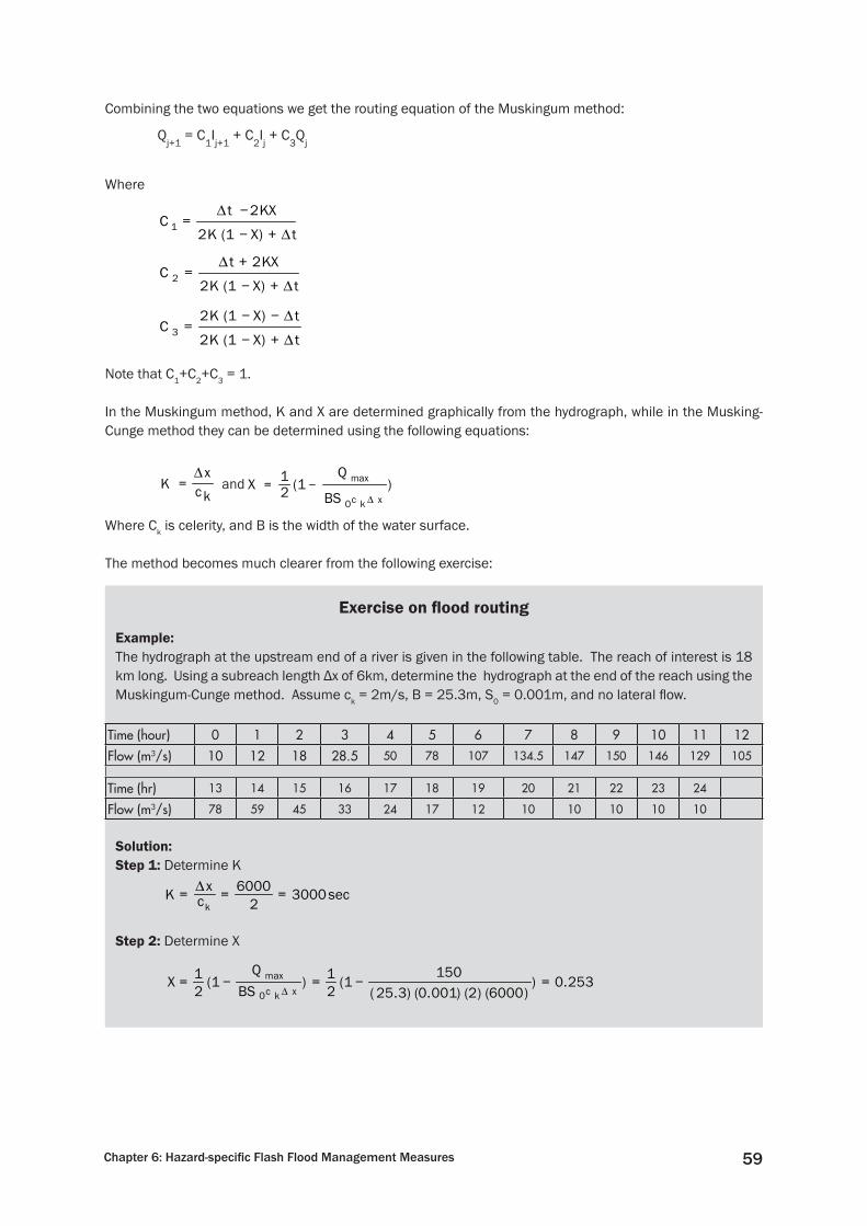
Where landslides can dam a riverBoth natural and anthropogenic factors can initiate dam-forming landslides. The most important natural processes in initiating dam-forming landslides are excessive precipitation (rainfall and snowmelt) and earthquakes (Figure 47).

Figure 47 shows that globally about 50% of dam-forming landslides are caused by rainstorms and snowmelt, about 40% by earthquakes, and only 10% by other factors. As volcanic eruptions are rare in the HKH region, the percentage of landslides causing dam formation due to rainfall, snowmelt, and earthquakes is higher.

Landslide dams form most frequently where narrow steep valleys are bordered by high rugged mountains (Table 18). This setting is common in geologically active areas where earthquakes and glacially steepened slopes occur, which is typical of the HKH region. These areas contain abundant landslide source materials, such as sheared and fractured bed materials, and experience triggering mechanisms which initiate landslides. Steep, narrow valleys require a relatively small volume of material to form dams; thus, even small mass movements present a potential for formation of landslide dams. Such dams are much less common in broad, open valleys. Most landslide dams are caused by falls, slides, and flows. Large landslide dams are often caused by complex landslides that start as slumps of slides and transform into rock or debris avalanches.

Modes of failure of landslide damsA landslide dam in its natural state differs from a constructed dam in that it is made up of a heterogeneous mass of unconsolidated or poorly consolidated material and has no proper drainage system to prevent piping

Talus

a. Fall b. Topple c. Slide

d. Spread

Original Position

Moving Mass

e. Flow

Figure 46: Types of landslides

Sour

ce: D

eoja

et a

l. 19

91


and control pore pressures. It also has no channelised spillway or other protected outlets; as a result, landslide dams commonly fail by overtopping, followed by breaching following erosion by the overflow water. In most documented cases, the breach has resulted from fluvial erosion of the landslide material, with headcutting originating at the toe of the dam and progressively moving upstream to the lake. When the headcut reaches the lake, breaching occurs. The breach commonly does not erode down to the original river level as many landslide dams contain some coarse material that armours the streambed locally. Smaller lakes can thus remain after dam failure.

Because landslide dams do not undergo systematic compaction, significant porosity and seepage through the dam can cause piping, which can lead to internal structural failure, although failure due to piping and seepage are quite rare compared to failure due to overtopping (Figure 48). In some cases piping and undermining of the dam can cause partial collapse of the dam, followed by overtopping and breaching.

A landslide dam with steep upstream and downstream faces and with high pore-water pressure is susceptible to slope failure. If the dam has a narrow cross-section or the slope failure is progressive, the crest may fail, leading to overtopping and breaching. Nearly all faces of landslide dams are at the angle of repose of the

0

10

20

30

40

50

60

Rains to rm and s no wm elt

E arthq uakes V o lc anic erup t io ns O ther

% o

f all

even

ts

Sour

ce: B

ased

on

Cost

a an

d Sc

hust

er 1

988

Figure 47: Causes of landslides that have formed dams

Table 18: Factors causing dam forming landslidesNatural Anthropogenic

High relief Deforestation

Undercutting of river banks Improper landuse

Weak geology - agriculture on steep slopes

High weathering - irrigation of steep slopes

Intensive rainfall - overgrazing

High snowmelt - quarrying

Poor sub-surface drainage Construction activities

Seismic activities


material or less; however, because they are formed dynamically, slope failures are rare. A special type of slope failure involves lateral erosion of the dam by a stream or river.

0

10

20

30

40

50

60

70

80

O v erto p p ing P ip ing S lo p e f ailure P hy s ic ally c o ntro lled

(d id not f a il)

% o

f all e

vent

s

Figure 48: Modes of failure of landslide dams

Sour

ce: B

ased

on

Cost

a an

d Sc

hust

er 1

988

Main triggers of landslides

Rainfall-induced landslidesRainfall is an important landslide trigger. There is a direct correlation between the amount of rainfall and the incidence of landslides.l Cumulative rainfall between 50-100 mm in one day and daily rainfall exceeding 50 mm can cause

small-scale and shallow debris landslides.l Cumulative two-day rainfall of about 150 mm, and daily rainfall of about 100 mm, have a tendency

to increase the number of landslides. l Cumulative two-day rainfall exceeding 250 mm, or an average intensity of more than 8 mm per hour

in one day, rapidly increases the number of large landslides.

Earthquake-induced landslidesEarthquakes can cause many large-scale, dam-forming landslides. Seismic accelerations, duration of shock, focal depth, and angle and approach of seismic waves all play a role in inducing landslides, but environmental factors such as geology and landforms play the most important role. This is why small earthquakes can sometimes induce more landslides than large earthquakes.

The type of slope and the slope angle have a great influence upon landslides. Landslides rarely occur on slopes less than 25°. The large majority of landslides occur on slopes with angles ranging from 30° to 50°.


Longevity of landslide damsLandslide-dammed lakes may last for several minutes or several thousands of years, depending on many factors, including volume, size, shape, sorting of blockage material, rates of seepage, and so on. External factors can also determine the longevity of landslide dams. For example, high stream inflow, intensive rainfall, or rockfall into the lake can cause rapid collapse of the dam.

There is very little time for action in the case of landslide dam formation. About 40% of landslide dams fail within a week of formation, and 80% fail within 6 months (Figure 49). It is clear that in the majority of cases there is not much time to mitigate the effects of dam failure unless a good local disaster management plan is in place.

Three factors govern the longevity of landslide dams: 1) rate of inflow to the impoundment; 2) size and shape of the dam; and 3) geophysical characteristics of the dam. The life of a dam can be shortened significantly due to the external factors mentioned above. The inflow rate is generally proportional to the upstream catchment area and is significantly greater during monsoon seasons. Landslide dams of predominantly soft, low-density, fine-grained, or easily liquified sediment lack resistance to erosion and are more susceptible to failure. Landslide dams comprised of larger and cohesive material are more resistant to failure. Poorly sorted materials with d15/d85 ratios greater than 5 are susceptible to internal erosion by piping (Sherard 1979).

Measures to minimise the risk of LDOFControl measures, such as the construction of spillways to drain the ponded water, have been attempted in various places around the world. Sometimes these measures have been successful in preventing an LDOF, in others overtopping has occurred before satisfactory control measures could be constructed. In some cases, the attempts themselves triggered floods that caused large-scale casualities. Here we focus on non-structural measures to mitigate LDOFs.

Landslide hazard assessmentThe first approach in LDOF mitigation is to identify places where the hazard can occur. This can be accomplished by preparing a landslide hazard map. If a landslide can occur in a narrow valley close to a stream, it could potentially cause a lake-forming dam. Additional analysis may provide an estimate of the volume of the dam, which together with the stream inflow rate can give an indication of the rate of lake level rise.

Hazard and risk mapping is done using 1) a simple qualitative method, which is based on experience and uses an applied geomorphic approach to determine parameters and their weightings, and scores and overlays of parameter maps for pre-feasibility level; 2) a statistical method score for the different parameters determined based on bi-variate and multivariate statistical analysis; 3) a deterministic method based on the properties of materials; and 4) social mapping using information derived from discussions with local people based on their experiences and feelings.

0

20

40

60

80

100

0 100 200 300 400

Age of dam at failure (days)

% o

f dam

s fa

iling

bel

ow

the

indi

cate

d ag

e

27% failures < 1 day

41% failures < 1 week

50 % failures < 10 days56 % failures < 1 month

80 % failures < 6 months86 % failures < 1 years

Figure 49: Length of time before failure of landslide dams (based on 73 case studies)

Sour

ce: B

ased

on

Cost

a an

d Sc

hust

er 1

988


The hazard may be classified as relative (assigning ratings to different factors contributing to hazard), absolute (deterministically derived, e.g., factor of safety), or monitored (actual measurement of effects, e.g., deformation along roads, rocks, and so on).

Relative hazard assessment generally follows these stepsdetermination of different factors contributing to slope instability ●

development of a rating scheme and scores for hazard probability ●

identification of elements at risk and their quantification ●

development of a rating scheme and scores for damage potential ●

construction of a hazard and risk matrix ●

mapping of hazard and risk ●

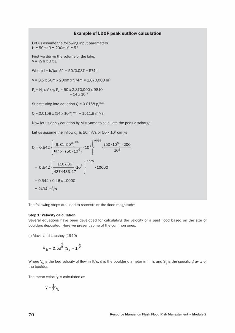
Estimation of downstream floodingInformed estimates about the magnitude of a potential flood are necessary in order to implement mitigation measures in areas downstream of the landslide-dammed lake. This can be done through techniques involving varying degrees of complexity. As, in most cases, the time between the dam formation and outburst is so short, a detailed analysis may not be possible and estimates will have to rely on simple techniques. Costa and Schuster (1988) suggested the following regression equation to estimate peak discharge of a LDOF:

Q = 0.0158Pe0.41

Where Q is peak discharge in cubic metres per second, and Pe is the potential energy in joules.

Pe is the potential energy of the lake water behind the dam prior to failure and can be calculated using the following equation:

Pe = Hd x V x g

Where Hd is the height of the dam in metres, V is the volume of the stored water, and γ is the specific weight of water (9810 Newton/m3).

Mizuyama et al. (2006) suggest the following equation for calculating peak discharge:

( )

6

33

1010

tan542.0

Bq

q

ghQ

in

in

⋅⋅

⋅⋅

=θ

0.5

0.565

Where Q is the peak discharge in m3/s; qin the inflow into the lake in cm3/s; g the gravitation acceleration (about 9.8 m/s2); h the dam height in metres; and θ the stream-bed gradient.

Figure 50 shows a schematic diagram of the input parameters and an example of calculating peak outflow is given below. The two methods give entirely different results as they include different parameters, the second method including more parameters than the first.

Sophisticated computer models are available to estimate the peak outflow of the LDOF and to route the flood along the river reach downstream of the lake. This will give the area and level of flooding, and can help in making decisions regarding relocating people or implementing structural mitigation measures.


Estimation of past floodsEstimation of past floods provides an idea of the magnitude of floods that are likely to affect a location. The slope-area method for estimating the magnitude of past floods is described above. Paleohydraulic reconstruction techniques can also provide estimates of past floods. These techniques reconstruct the velocity of the flow, depth, and width of the channel during the flood based on the size of boulders deposited by the flood. Details are given in Costa (1983). These estimates provide a basis for identifying the magnitude of a past flood and for assessing potential future hazard and risk.

h

qin

a.

b.

B

q in

Θ

Figure 50: A schematic diagram showing the parameters used in calculating peak outflow discharge: a. isometric view; and b. cross-section.


The following steps are used to reconstruct the flood magnitude:

Step 1: Velocity calculationSeveral equations have been developed for calculating the velocity of a past flood based on the size of boulders deposited. Here we present some of the common ones.

(i) Mavis and Laushey (1949)

( ) 2

194

15.0 −= gb SdV

Where Vb is the bed velocity of flow in ft/s, d is the boulder diameter in mm, and Sg is the specific gravity of the boulder.

The mean velocity is calculated as

VV b3

1_=

Example of LDOF peak outflow calculation

Let us assume the following input parametersH = 50m; B = 200m; q = 5°

First we derive the volume of the lake:V = ½ h x B x L

Where l = h/tan 5° = 50/0.087 = 574m

V = 0.5 x 50m x 200m x 574m = 2,870,000 m3

Pe = Hd x V x g, Pe = 50 x 2,870,000 x 9810 = 14 x 1011

Substituting into equation Q = 0.0158 pe0.41

Q = 0.0158 x (14 x 1011) 0.41 = 1511.9 m3/s

Now let us apply equation by Mizuyama to calculate the peak discharge.

Let us assume the inflow qin is 50 m3/s or 50 x 106 cm3/s

( )6

6565.0

36

5.03

10200)1050(

10)1050(tan5

5081.9542.0

⋅⋅⋅

⋅⋅⋅

⋅=Q

1000010

17.4374433

36.1107542.0

565.03 ⋅

⋅=

= 0.542 x 0.46 x 10000

= 2494 m3/s


(ii) Strand (1977)

21

51.0 dVb=

Where Vb is velocity of flow in ft/s and d is the boulder diameter in mm. The mean velocity of flow is derived in the same way as for Mavis and Laushey (1949).

(iii) Williams (1983)

5.0_

065.0 dV =

Where V_

is the mean velocity of flow (m/s) and d is the diameter of the boulder in mm.

Step 2: Depth CalculationThe next step is to calculate the mean depth of the flow. Again several methods are available for calculating the mean depth.

(i) Manning’s equation

5.1__)(

SnVD =

√

Where D_

is mean depth, n is the roughness coefficient, and S the slope.

(ii) Costa (1983)

In this method, a nomogram developed by Costa (1983; Figure 51) is used to derive the mean depth.

(iii) Sheild (1936)

SD fd S /)(.

_γγθ −=

Where θ is dimensionless shear stress (use 0.02), γf

= 1070 kg/m3, and γs= 2700

kg/m3.

(iv) Williams (1983)

SfD γτ/

_=

d 0.117.0=τ

Where t is shear stress (N/m2), d is diameter of boulder (mm), and g is the specific weight of water.

Step 3: Width calculationThe width is determined using an iterative method. A straight reach for cross-section (neither expanding nor contracting) is selected. The site should not be abnormally wide, narrow, steep, or flat. At least one, and preferably both, valley walls should be bedrock. The site should be close to the depositional site. Select at least two cross-sections spaced about one valley-width apart. No major tributaries should enter the main channel between the cross-sections.

10

5

1.0

0.5

0.150 100 500 1000 5,000 10,000

0.005

0.01

0.02

0.050.10

d (mm)

D (m

)

Figure 51: Graph to predict average depth ( D_

) of past flood from boulder size (d) and channel slope. The numbers beside the lines indicate the channel slopes.

Sour

ce: F

rom

Cos

ta 1

983


Once the cross-sections have been plotted, draw a line to represent the estimated top width of the cross-section (Figure 52). Using a planimeter or a digitiser, calculate the area of the cross-section and divide it by the top width of the cross-section. If the value deviates from the estimated depth from Step 2, draw a new top-width line and repeat the process until the two values agree. Now, calculate the cross-sectional area ‘A’ for the final top-width.

Step 4: Calculation of dischargeKnowing the average velocity from Step 1 and the cross-sectional area from Steps 2 and 3, a single discrete estimate of flood discharge (Q) can be made using the following equation:

AVQ .

_=

Land use regulationThe increasing hazard and risk of LDOFs are a result of unregulated use of land and investment in flood-prone areas for infrastructure development such as buildings and roads. Public buildings such as schools are being constructed even on small islands between river distributaries, and houses are encroaching on natural river channels. Figures 53 and 54 provide evidence of such practices. In this context, the most effective way to mitigate LDOFs is to avoid activities that can cause landslides, particularly in narrow valleys where landslides can result in lake-forming dams. In such areas, development activities should be located on stable ground and landslide-susceptible areas should be used for open space or for low-intensity activities such as parkland or grazing. Land use controls can prevent hazardous areas from being used for settlements or as sites for important structures. The controls may also involve relocation away from the hazardous area, particularly if alternative sites exist. Restrictions may be placed on the type and amount of building that may take place in high-risk areas. Activities that might activate a landslide should be restricted. Where the need for land is critical, expensive engineering solutions for stabilisation may be justified. Building codes and design standards are also necessary.

Financial measuresGovernments may assume responsibility for the cost of repairing damage from LDOFs as well as efforts to prevent them. Insurance programmes may reduce losses from LDOF by spreading the expenses over a larger base and including standards for site selection and construction techniques. Financial measures may be used to relocate people/activities from a landslide-prone area.

A

W

0

1

2

3

4

0 5 1 0 1 5 2 0 2 5 3 0 3 5 4 0

De

pth

(m

)

D istance (m)Figure 52: Top-width (W) and cross-section area (A) for calculation of depth by the iterative method

73

N.R

. Kha

nal,

TU, N

epal

Figure 53: Damage resulting from the 1998 LDOF in Syangja, central Nepal

74

Early warning systemsEarly warning systems (EWSs) can be an effective measure to mitigate the impacts of LDOFs, particularly in saving life and property. Depending on the situation, a variety of early warning systems can be implemented. As the lifetime of landslide dams is often quite short, a sophisticated system may not be possible. In many cases the best option is to implement a community-based EWS. This may consist of placing people at strategic locations starting from the dam site to the distance downstream up to which the LDOF can have an impact. Each location should have visual contact with the person just upstream and downstream. EWSs as part of a monitoring, warning, and response system (MWRS) have been described in Chapter 5.

6.3 Glacial Lake Outburst FloodUnderstanding the processGlaciers A glacier is a large flowing ice mass. The flow is an essential property in defining a glacier. Usually a glacier develops under conditions of low temperature caused by cold climate, although this in itself is not sufficient to create a glacier. An area in which the total depositing mass of snow exceeds the total mass of snow melting during a year is defined as an accumulation area. Thus, snow layers are piled up year after year because the annual net mass balance is positive. As a result of the overburden pressure due to weight, compression occurs in the deeper snow layers, and the density of the snow layers increases. Snow becomes impermeable to air a critical density of approximately 0.83 g/cm3. The impermeable snow is called ice. Ice has a density ranging from 0.83 to a pure ice density of 0.917 g/cm3. Snow has a density range from 0.01 g/cm3 for fresh layers just after snowfall to ice at a density of 0.83 g/cm3. Perennial snow with high density is called ‘firn’. In the glacier, the snow changes to ice below a certain depth. When the thickness of ice exceeds a certain critical depth, the ice mass starts to flow down along the slope by plastic deformation and slides along the ground driven by its own weight. The lower the altitude, the warmer the climate. Below a critical altitude, the annual mass of deposited snow melts completely, the ‘end’ of the glacier. Here, snow disappears during the hot season and may not accumulate year after year. This area with a negative annual mass balance is

Figure 54: A school located on a small island between distributaries of the Bagmati River in Kavre District, Nepal

N.R

. Kha

nal,

TU, N

epal


defined as the ablation area. A glacier is divided into two such areas, the accumulation area in the upper apart of the glacier and the ablation area in the lower part. The boundary line between them is defined as the equilibrium line, where the deposited snow mass is equal to the melting mass in a year. Ice mass in the accumulation area flows down into the ablation area and melts away. Such a dynamic mass circulation system is defined as a glacier. There are different types of glaciers, such as ice sheet, ice field, ice cap, outlet glacier, valley glacier, mountain glacier, glacieret and snowfield, ice shelf, and rock glacier.

A glacier can change in size and shape due to the influence of climate change, advancing when the climate changes to a cool summer and heavy snowfall in winter and the monsoon season. As the glacier advances, it expands and the terminus shifts to a lower altitude. A glacier retreats when the climate changes to a warm summer and less snowfall. As the glacier retreats, it shrinks and the terminus climbs up to a higher altitude. Thus, climatic change results in a glacier shifting to another equilibrium size and shape.

Formation of glacial lakesThe formation and growth of glacial lakes is closely related to deglaciation. Shrinkage of glaciers is a widespread phenomenon in the HKH region at present, closely associated with climate change. The world has experienced many episodes of glacial and inter-glacial periods, during which glaciers advanced and retreated dramatically. A globally synchronous re-advance of glaciers occurred during the so-called ‘Little Ice Age’ (LIA), which prevailed from the middle of the 16th Century to the middle of the 19th Century16. The climate has gradually warmed since the end of the LIA, accompanied by the retreat of glaciers. Glacial retreat has accelerated in recent decades, generally attributed to human-induced increase of greenhouse gasses in the atmosphere and resultant overall warming. Valley glaciers generally contain supra-glacial ponds, which grow bigger and merge with a warming climate. This process is accelerated by rapid retreat of glaciers. As glaciers retreat, they leave a large void behind, and meltwater is trapped in the depression previously occupied by glacial ice thus forming a lake. Figure 55 shows the rapid growth of Tsho Rolpa lake in Nepal as an example.

1957-59

1960-68

1975-77

1979

1983-84

1988-90

1994

1997

2002

0.61 km2

0.62 km2

0.78 km2

0.80 km2

1.02 km2

1.16 km2

1.27 km2

1.39 km2

1.65 km2

1.76 km2

0 1 2 3 km

0.23 km2

1974

1972

Figure 55: Development of Tsho Rolpa glacial lake, Nepal

16 It was initially believed that the LIA was a global phenomenon, but recent studies question this. The beginning and end of the LIA is also a matter of debate among the scientific community.


Moraine damsGlacial lakes are retained by the moraine dams created by the glacier during its advance stage. Debris falling on glaciers due to weathering of surrounding slopes and materials collected from the bottom of the glacier, are dumped loosely at the end of glaciers forming a terminal or end moraine (1 in Figure 56) and at the side of the glaciers forming lateral moraines (2 in Figure 56). These moraine dams are structurally weak and unstable, and undergo constant changes due to slope failure, slumping, and so on. This process can be aggravated; there is a potential for catastrophic failure, causing a glacial lake outburst flood (GLOF).

Causes of failure of moraine damsA moraine dam may break as the result of the action of some external trigger or by self-destruction. A huge displacement wave generated by a rockslide or snow/ice avalanche from the glacier terminus (Figure 57, bottom) or hanging glaciers (5 in Figure 56) falling into the lake, may cause the water to overtop the moraines, creating a large breach and eventually causing dam failure (Ives 1986). Earthquakes may also trigger a dam break depending upon magnitude, location, and characteristics. Self-destruction is caused by the failure of the dam slope and seepage from the natural drainage network of the dam (Figure 57, top). Richardson and Reynolds (2000) analysed 26 GLOF events in the Himalayas in the 20th Century and concluded that a majority of the moraine dam failures were triggered by overtopping by a displacement wave caused by ice avalanches into the lake from hanging or calving glaciers (Figure 58).

Impacts of GLOFsA GLOF is characterised by a sudden release of a huge amount of lake water, which in turn rushes downstream along the stream channel in the form of dangerous flood waves. These flood waves are comprised of water mixed with morainic materials and can have devastating consequences for downstream riparian communities, hydropower stations, and other infrastructure. Rushing water erodes both banks of the river and causes landslides from the steep slopes along the river channel. A moraine-dammed lake outburst results in a greater rate of water release than an ice-dammed lake burst, as in the latter case the release of water occurs

1

2

2

3

4

55

6

6

6

4

Box 1

Box 2

Figure 56: Schematic view of a typical glacial lake in the Himalayas. 1) end moraine; 2) lateral moraine; 3) glacial lake; 4) glacier terminus; 5) hanging glacier; 6) talus slope (rock fall). Details of Boxes 1 and 2 are shown in Figure 57


Figure 57: Detailed view of frontal part of the glacial lake, Box 1 in Figure 56 (top), and terminus of the parent glacier, Box 2 in Figure 56 (bottom)


over a prolonged duration, sometimes days, whereas in the former case the outburst is almost instantaneous, occurring within minutes to hours (Figure 59; Yamada 1998). The magnitude of the GLOF and the corresponding damage depend on the surface area and volume of the lake, release rate of water, and natural features of the river channel. The discharge rates of such floods are typically several thousand cubic metres per second. The peak discharge during the outburst of Zhangzangbo GLOF in 1981 was estimated to be around 16,000 m3/s (Xu 1985). The peak outflow of the Dig Tsho GLOF was estimated to be 5,610 m3/s (Shrestha et al. 2006).

Depending on the channel topography and morphology, the peak flood will attenuate along the river channel. Figure 60 shows some examples of attenuation of peak flood discharge with distance along the river channel. While the inundation caused by the GLOF is generally not extensive, it can be quite destructive due to the high velocity of the flood waves. Flood velocities during a GLOF can be as high as 10m/s, which is high

0

10

20

30

40

50

60

O v erto p p ing d ue to ic e av alanc he

S eep ag e O v erto p p ing d ue to ro c k av alanc hes

M elt ing Ic e-c o re Unkno wn

% o

f tot

al e

vent

s

Figure 58: Causes of recorded glacial lake outburst floods in the Himalayas

Very steep rising limb

Steep fallinglimb

Slow rising limb

Time (days)

Dis

char

ge(m

3 /s)

0 1 2

12

Figure 59: Outburst of moraine-dammed lake (1) and ice-dammed lake (2) (Yamada 1998)

Sour

ce: B

ased

on

Ric

hard

son

and

Reyn

olds

200

0

0

2000

4000

6000

8000

10000

12000

14000

16000

18000

0 10 20 30 40 50 60

Distance from lake (km)

Peak

dis

char

ge (m

3 /s)

Zhangzangbo

Imja (modelled)

Dig Tsho(modelled)

China-Nepalborder

Figure 60: Examples of attenuation of peak flood along the river channel

Sour

ce: X

u 19

85; S

hres

tha

et a

l. 20

06


enough to destroy bridges and settlements and wash away highways and agricultural lands. GLOFs typically contain a large amount of debris mixed with water, which increases the destructive power of the flood. During the recession of the flood, the debris settles on the valley floor, making it useless for agriculture and other uses for a long time (Figure 61).

Which glacial lakes can burst out?ICIMOD has identified more than 8,800 glacial lakes in the HKH region (Table 19; ICIMOD 2007). Most of these lakes do not pose any danger of outburst, but a small number do. These are called ‘potentially dangerous lakes’. From the study of past GLOFs in the region, it is clear that GLOF events are clustered around the eastern Himalayas in Nepal, Bhutan, and Tibet. For GLOF risk management it is important to know which lakes pose a danger of outburst. Some 20 potentially dangerous lakes were identified in Nepal and 24 in Bhutan.

Methods to determine whether a lake is potentially dangerous can range from simple desk-based to complicated methods, involving many highly specialised field investigations. A potentially dangerous lake can be identified based on the following factors.

a. b. c.

d.

Figure 61: Impacts of GLOF on the river channel of the Madi River in central Nepal: a. before; and b. after a small GLOF on 15 August 2003; c. deposition of debris in the river channel due to Dig Tsho GLOF of 1985; and d. eroded banks of Tamur River after the Nagma GLOF

Sour

ce: a

. & b

. Ast

er im

ages

; c. A

run

B. S

hres

tha;

and

d. M

ool e

t al.

2001

Table 19: Glacial lakes in the Hindu Kush-Himalayan region

River basinsGlacial lakes

Total number

Area (km2)

Pakistan

Indus Basin 2420 126.35

India

Himachal Pradesh 156 385.22

Uttaranchal 127 2.49

Tista River 266 20.2Tibet Autonomous Region of the Peoples’ Republic of China (sub-basins of Ganges) 824 85.19

Nepal Himalaya 2323 75.7

Bhutan Himalaya 2674 106.87

Total within the study area 8790 799.49Source: ICIMOD 2007


Volume and rise in lake water levelAn outburst of a relatively small lake may not have a significant impact. Lakes smaller than 0.01 km3 in volume are not considered potentially dangerous. The dynamics of the water level are also important, as increase in water level increases the hydrostatic pressure on the moraine dam and may result in the collapse of the dam.

Activity of glacial lakeThe activity of the lake is very important for analysing the potential danger. Rapidly increasing lake size indicates a high possibility of a GLOF. Similarly, a lake boundary and outlet position that is dynamic in nature also indicates a high risk.

Position of lakePotentially dangerous lakes are generally at the lower part of the ablation area of the glacier near the end moraine. The parent glacier must be sufficiently large to create a dangerous lake environment. Regular monitoring needs to be carried out for such lakes with the help of multi-temporal satellite images and field investigations.

Moraine dam conditionThe condition of the moraine damming the lake determines the lake stability. The possibility of outburst due to collapse of the moraine dam increases if:

the dam has a narrow crest area ●the dam has steep slopes ●the dam is ice cored ●the height above the valley floor is high ●there are instabilities on the slopes of the dam ●there is seepage through the moraine dam ●

Condition of parent glacier and glaciers on the peripheryThe terminus of the parent glacier in contact with the lake experiences calving due to development of thermo-karsts on the lower part of the terminus and exploitation of crevasses on the glacier. A large drop of glacial ice can cause a displacement wave sufficient to travel across the lake and cause overtopping of the moraine dam. A steep parent glacier or glacier on a side valley can cause ice avalanches into the lake. Such ice avalanches also cause displacement waves capable of overtopping moraine dams.

Physical condition of surroundingsUnstable mountain slopes with the possibility of mass movements around the lake, and snow avalanches, can cause displacement waves and overtopping of moraine dams. Smaller lakes located at higher altitudes sometimes pose a danger to a glacial lake of concern. Outbursts of such high-altitude lakes might drain into the glacial lake, causing overtopping and consequent failure of the moraine dam.

Measures to minimise the impacts of GLOFsEarly recognition of riskThe most effective way to minimise the risk of a GLOF is to understand the risk early so that appropriate measures can be taken in a timely and cost-effective manner. This involves investigation of the factors listed above. Many of these can be investigated without field studies by using remote sensing and GIS technologies. The first step is to inventory the glaciers and glacial lakes in the region. While preparing the inventory of glacial lakes, parameters that can be derived remotely can be entered as attributes. Then a logical command in the GIS software can identify potentially dangerous lakes in the area of interest.

Annex 6 describes a methodology17 for preparing an inventory of glaciers and glacial lakes and automatically identifying those that are potentially dangerous. Annex 6 is based on image processing and the GIS software 17 The annex is part of an unpublished manual developed by P.K. Mool and S.R. Bajracharya of ICIMOD.


ILWIS18 3.2 developed by the International Institute for Geo-Information Science and Earth Observation (ITC), Netherlands. Example data for conducting the exercise accompanies the Annex. Following desk-based identification of the potentially dangerous lakes, field investigations can be conducted on the short-listed lakes.

RGSL (2003) has suggested criteria for defining the GLOF hazard of glacial lakes (Table 20), and a hazard rating based on the score (Table 21). A glacial lake scoring higher than 100 is potentially dangerous and an outburst can occur at any time. Glacial lakes should be monitored regularly to establish the status of the criteria listed in Table 20. Here we present some guidelines for determining each of the criteria.

Volume of lake: The volume of the lake can be established by bathymetric survey; there are two common methods. The first is to directly measure the depth when the lake is frozen. A grid of measurement points is pre-determined and holes are bored through the ice layer, through which depth sounding is done. The measurement points are interpolated to get the total volume of the lake. Another method gaining more popularity is measurement using echo-sounders. Echo-sounders are mounted on a small boat, which travels along pre-established transects on the lake. The positions along the transects are given by an online GPS connected to the echo-sounder (e.g., Shrestha et al. 2004; Figure 62). This method can give a relatively dense measurement in a short time. The volume thus derived can be related to the surface area of the lake and after a number of measurements a volume:area relationship can be established. The surface area can be measured more frequently either by field survey or by remote sensing analysis, and the volume derived from the volume:area relationship.

Calving risk from ice cliff: The status of the parent glacier terminus has to be routinely monitored in the field. The geometry and size of the terminus can give useful information regarding the possibility of large displacement waves. A high and overhanging ice-cliff can be conducive to ice calving, potentially causing large displacement waves. A debris/ice apron in front of the ice-cliff (Figure 57, bottom) reduces the chance of generating a large displacement, even when ice calving occurs. Often ice termini have a series of crevasses (Figure 63). These crevasses are exploited during ice calving, thus monitoring crevasses and the structure of the ice cliff can be useful in predicting the size of future ice calving. The terminus and crevasses can be

Table 20: Empirical scoring system for moraine-dammed glacial lake outburst hazard (RGSL 2003)

Criteria affecting hazard/score 0 2 10 50

Volume of lake N/A Low Moderate Large

Calving risk from ice cliff N/A Low Moderate Large

Ice/rock avalanche risk N/A Low Moderate Large

Lake level relative to freeboard N/A Low Moderate Full

Seepage evident through dam None Minimal Moderate Large

Ice-cored moraine dam with/without thermokarst features None Minimal Partial >Moderate

Compound risk present None Slight Moderate Large

Supra/englacial drainage None Low Moderate Large

Table 21: Hazard rating on the basis of the empirical scoring system (RGSL 2003)

0 50 100 125 150+

Zero Minimal Moderate High Very High

An outburst can occur any time

18 An open source version, ILWIS 3.4 Open, can also be used. It is freely downloadable from <http://52north.org/index.php?option=com_projects&task=showProject&id=30&Itemid=127>


monitored by repeat photography. High-resolution satellite imagery can provide some information on the crevasses, and field surveys can provide information on the height of the ice cliff.

Ice/rock avalanche risk: Ice avalanches from hanging glaciers and rock avalanches from weathered slopes into lakes can cause large displacement waves capable of overtopping moraine dams and causing their failure. Ice and rock avalanche areas have to be monitored regularly for early detection of large avalanches. This can be done through a combination of visual inspection on the ground and high-resolution satellite imagery (Figure 64; 5 in Figure 56).

Lake level relative to freeboard: High water level and low freeboard means that even a relatively small displacement wave can overtop the moraine dam. The dynamics of the lake water level have to be observed continually. This can be done by establishing a lake water level measuring station (Figure 65). The station can have a simple level gauge monitored regularly by a gauge reader, or could be an automatic recorder with a water level pressure sensor and data logger. The water level observation can be supplemented by discharge measurements, which will give important information on the outflow of the lake.

Seepage evident through dam: Seepage through a moraine dam may indicate piping inside the dam leading to dam failure. Seepage could also be due to rapid melting of dead ice inside the moraine dam, which can lead to formation of a void inside the dam and consequently its collapse. The height of the seepage outlet and seasonal fluctuation of the seepage quantity have to be monitored. Seepage due to infiltrated precipitation is seasonal and does not pose a serious threat to the integrity of the dam.

Ice-cored moraine dam with/without thermokarst features: Thermokarst refers to voids in the moraine dam caused by rapid melting of buried ice blocks (Figure 56, Box 1). Thermokarsts reduce the structural stability of the moraine dam against the hydrostatic pressure of the lake water. Slumping and subsidence due to collapse of a thermokarst may cause overtopping of a moraine dam, leading to its collapse. Features on the moraine like slumping and subsidence have to be monitored regularly. This can be done visually or by conducting a detailed topographic survey of the area of concern. Specialised techniques such as ground penetrating radar survey or electro-resistivity survey have to be conducted for 3-dimensional mapping of the buried ice.

Supra/englacial drainage: Parent glaciers generally contain several supra-glacial lakes (Figure 56, Box 2; Figure 57, bottom; Figure 66) and englacial channels. Occasionally these ponds drain though the englacial channel into the glacial lake. Similarly, other lakes at higher altitude might suffer outbursts that might drain into the glacial lake. If the volume of the water released is significant, it might cause overtopping of the moraine dam. Supra-glacial ponds and high altitude lakes have to be monitored regularly. Satellite images

Transducer

Transducer

Echo SounderGPS AntennaOutboard

MotorInflatableBoat

GPS Antenna

Echo Sounder

a. b.

c.

Figure 62: a. Set-up for bathymetric survey; b. schematic set-up diagram, top view; c. schematic setup diagram, side view


Glacial lake

Crevasses

Glacial lake

Ice cli�

Crevasses

Figure 63: Terminus of the Trakarding glacier, the parent glacier of Tsho Rolpa glacial lake, Nepal, showing a series of crevasses in plan view and frontal view

Sour

ce: G

oogl

e Ea

rth

(top)

; Aru

n B.

Shr

esth

a (b

otto

m)

can provide multi-temporal information on the development of supra-glacial ponds and high altitude lakes in the surrounding areas.

Estimation of peak outflow discharge: Sophisticated computer models are available to estimate the peak discharge of a GLOF. Due to limited resources and expertise, it is not always possible to do a detailed modelling exercise. A simple method can also provide a reasonably good estimate of the outburst magnitude.

Costa and Schuster (1988) suggested the following equation for predicting peak outflow discharge from a GLOF: Q = 0.00013(Pe)

0.60

Where Q is peak discharge in m3/s, and Pe is potential energy in joules.

Pe is the energy of the lake water behind the dam prior to failure and can be calculated using the equation:

Pe = Hd x V x g

Popov (1991) suggested the following equation for predicting flash flood peak discharge due to glacier outburst:

Q = 0.0048V 0.896


Hanging glaciers

Lake

Hanging glaciers

Lake

Figure 64: Hanging glaciers near a glacial lake: frontal view (top) and plan view (bottom)

Sour

ce: G

oogl

e Ea

rth

(bot

tom

); Ar

un B

. Shr

esth

a (to

p)


The peak discharge depends on the volume of the glacial lake (V). The lake volume is generally not available unless a detailed bathymetric survey has been conducted. The surface area of the lake, however, can be easily derived from maps of satellite imageries. The volume can then be calculated using the following formula suggested by Huggel et al. (2002):

V = 0.104A 1.42

Peak outburst depends on the nature of the outburst, i.e., the duration of the outburst, the nature of the outburst hydrograph, and the size and geometry of the dam breach. In the simple approach, a triangular breach hydrograph is assumed and the duration of the outburst is assumed as 1000s. Huggel et al. (2002) suggest that most outbursts last between 1000 and 2000 seconds, and the peak discharge is calculated by:

tVQ 2=

Figure 65: An automatic weather station equipped with a lake water-level recorder, Lirung, Nepal

Figure 66: Parent glaciers of Imja Lake, Nepal, showing supra-glacial ponds

Glacial lake Supra-glacialponds

Sour

ce: G

oogl

e Ea

rth


Estimation of area that can be impacted by a GLOFThe hazard assessment should include a rough estimate of the area potentially affected by a lake outburst. A worst-case scenario is generally followed for delineating the area that could be affected. The runout (travel) distance of an outburst is related to the amount of debris available to be mobilised. Outburst floods with a higher content of solid material form debris flows and stop abruptly, whereas GLOFs with predominantly water attenuate more gradually.

To roughly estimate the maximum affected area, the peak discharge is used to estimate the overall slope of the outburst flood (the average slope between the starting and the end points of an outburst event). Figure 67 shows the relationship between maximum outflow discharge and critical runout slope. For instance, an outflow discharge of 100 m3/s gives a critical slope of 2.75.

Figure 68 shows the profile of a river channel. The critical slope of 2.75 means the flood will have an effect up to a distance of 20 km (point 3 in Figure 68).

GLOF risk mappingGLOF risk mapping is an important tool to understand the areas likely to be impacted by a GLOF and to understand the vulnerability of those areas, and will help in planning mitigation measures. Detailed descriptions of GLOF risk mapping can be found in Shrestha et al. (2006) and Bajracharya et al. (2007 a and b). The process involves estimating the discharge hydrograph at the outlet (breach). This can be done using dam break models or by simple calculation assuming the breach size and the lake drawdown rate. The hydrograph is routed through the river reach to find the peak discharge and flood height at the locations of interest. An inundation map is prepared by overlaying the flood height over the terrain map. Overlaying a socioeconomic vulnerability map based on the information mentioned in Chapter 4 will give the risk map of the area. See Chapter 4 for details on risk assessment.

Terrain AnalysisGLOF is a complex phenomenon involving floods, sediment transport, debris flows, landslides, and others, which cannot be accurately predicted or foreseen. Terrain analysis can be a good indicator of the magnitude of what might happen during a GLOF event. Terrain analysis is a good tool to verify the results of a hazard map. Bajracharya et al. (2007b) provides a detailed description of terrain analysis.

2.75 o 100 m 3/s

2

1

3

Elev

atio

n (m

asl)

0

1000

2000

3000

4000

5000

6000

0 5000 10000 15000 20000

Lake

Distance from the lake (metres)

5.5 o 25 m 3/s

18 o 2 m 3/s

Figure 68: Longitudinal profile of a stream and runout distances for different peak outfow discharges

?

Criti

cal s

lope

(o C)

Max discharge (m3/s)

Debris �owFlood wave

2,75

100

Figure 67: Relation between peak discharge and overall slope of runout distance of lake outburst based on data from the Alps

Sour

ce: B

ased

on

Hug

gel e

t al.

2002

; Hug

gel e

t al

. 200

4

6.1 intense rainfall flood - himaldoc -...

Documents