62 - univie.ac.at · () fix t arian v in as a subspace. w no e w shall lo ok at the tation represen...

Doc.Math. J. DMV 61

Hopf-Bifurcation in Systems with Spherical Symmetry

Part I : Invariant Tori

Christian Leis

Received: February 10, 1997

Revised: April 4, 1997

Communicated by Bernold Fiedler

Abstract.

A Hopf-bifurcation scenario with symmetries is studied. Here, apart from

the well known branches of periodic solutions, other bifurcation phenomena

have to occur as it is shown in the second part of the paper using topological

arguments. In this �rst part of the paper we prove analytically that invariant

tori with quasiperiodic motion bifurcate. The main methods used are orbit

space reduction and singular perturbation theory.

1991 Mathematics Subject Classi�cation: 58F14, 34C20, 57S15

Contents

1 Introduction 62

2 Representation of the group O(3) � S

1

on V

2

� iV

2

64

3 Restriction to Fix(Z

2

; 1) 69

3.1 Poincare-series, invariants, and equivariants . . . . . . . . . . . . . . . 69

3.2 Orbit space reduction . . . . . . . . . . . . . . . . . . . . . . . . . . . 73

3.3 Lattice of isotropy subgroups . . . . . . . . . . . . . . . . . . . . . . . 76

3.4 Critical points of the reduced vector �eld . . . . . . . . . . . . . . . . 81

3.5 Stability of the critical points of the reduced vector �eld . . . . . . . . 91

3.6 Fifth order terms . . . . . . . . . . . . . . . . . . . . . . . . . . . . . . 96

3.7 Singular perturbation theory . . . . . . . . . . . . . . . . . . . . . . . 99

3.8 Invariant tori . . . . . . . . . . . . . . . . . . . . . . . . . . . . . . . . 104

3.9 Stability of the invariant tori . . . . . . . . . . . . . . . . . . . . . . . 109

Documenta Mathematica 2 (1997) 61{113

62 Christian Leis

1 Introduction

An interesting problem in the theory of ordinary di�erential equations is the gen-

eralization of the two dimensional Hopf-bifurcation to higher dimensional systems

with symmetry. In this connection, [GoSt] and [GoStSch] investigated problems on

a vector space X that can be decomposed into a direct sum of absolutely irreducible

representations of the group O(3) of the formX = V

l

� iV

l

. Here V

l

denotes the space

of homogeneous harmonic polynomials P : R

3

! R of degree l. This is the simplest

case where purely imaginary eigenvalues (of high multiplicity) in the bifurcation

point are possible. Using Lie-group theory, the authors showed the existence of

branches of periodic solutions with certain symmetries. Here in addition to the

spatial O(3)-symmetry a temporal S

1

-symmetry occurs. This symmetry corresponds

to a time shift along the periodic solutions. In order to obtain their results, the

authors made a Lyapunov-Schmidt-reduction on the space of periodic functions.

The reduced system then has O(3) � S

1

-symmetry and solutions correspond to

periodic solutions of the original system with spatial-temporal symmetry. Under

certain transversality assumptions, periodic solutions with symmetry

�

H � O(3)� S

1

bifurcate if Dim Fix(

�

H) = 2 for the induced representation of the group O(3)� S

1

on

the space X (cf. [GoSt] resp. [GoStSch]). [Fi] has shown that it is su�cient that

�

H

is a maximal subgroup for periodic solutions with symmetry

�

H to bifurcate. Using

these methods, only the existence of periodic solutions can be investigated. Via

normal form theory (cf. [EletAl]) one gets O(3) � S

1

-equivariant polynomial vector

�elds up to every �nite order for our systems. This additional S

1

-symmetry is due to

the fact that the normal form commutes with the one parameter group e

L

T

t

which

is generated by the linearization L in the bifurcation point. For a Hopf-bifurcation

L has purely imaginary eigenvalues (of high multiplicity) and the group generated is

a rotation. [IoRo], [HaRoSt] and [MoRoSt] did analytic calculations for the normal

form up to �fth order in the case l = 2. They gave conditions for the stability of

the �ve branches of periodic solutions predicted by [GoSt] resp. [GoStSch] in terms

of coe�cients of the normal form. Quasiperiodic solutions found by [IoRo] in the

normal form up to third order can not be con�rmed in this paper. We shall show a

mechanism for quasiperiodic solutions to bifurcate in the �fth order.

Investigating the normal form due to [IoRo], one �nds a region in parameter space

where two of the branches of periodic solutions bifurcating supercritically are stable

simultaneously. Using topological methods, [Le] showed that we have the following

alternative in this region in parameter space: Either besides the known branches of

periodic solutions other invariant objects bifurcate or recurrent structure between

the di�erent invariant sets (e.g. between the di�erent group orbits of periodic

solutions and the trivial solution) exists. Actually the results of these topological

investigations were the starting point of analytical e�orts to �nd other solutions (or

recurrent structure) in this paper. In order to get our results, we shall proceed as

follows.

First the representation of the group � = O(3) � S

1

on the ten dimensional space

X = V

2

� iV

2

is introduced. The lattice of isotropy subgroups of this representation

is given according to [MoRoSt] and the results of [IoRo] are quoted. The smallest

invariant subspace containing both solutions that are stable simultaneously has

isotropy � = (Z

2

; 1).


Invariant Tori 63

Then our considerations are being restricted to this six dimensional subspace.

The normaliser of � is N(�) = O(2) � S

1

� �. This is the biggest subgroup of �

leaving Fix(�) invariant as a subspace. Now we shall look at the representation of

N(�)

�

on Fix(�).

Dealing with di�erential equations with symmetries, one has to deal with group

orbits of solutions because a solution x(t) gives rise to solutions x(t) with 2 �.

This redundancy, induced by the action of the group, will be removed by identifying

points that lie on a group orbit. I.e. one studies the orbit space that is homeomorphic

to the image of the Hilbert-map � : Fix(�) ! R

k

: z ! �

i

(z) (cf. [La2] and [Bi]).

Here k denotes the minimal number of generators of the ring of

N(�)

�

invariant poly-

nomials P : Fix(�) ! R and �

i

; i = 1; : : : ; k, is such a system of generators. Thus

the original di�erential equation is reduced to a di�erential equation on �

�

Fix(�)

�

of

the form _� = g(�); � = (�

1

; : : : ; �

k

). In order to perform this reduction for a given

equation, one, �rst of all, has to know the number of independent invariants and

equivariants for a given representation. Then one, actually, has to calculate them.

Statements on the number of independent invariants and equivariants and possible

relations between them are given by the Poincaré-series. These are formal power

series

P

1

i=0

a

i

t

i

in t. Here a

i

denotes the dimension of the vector space of homoge-

neous invariant polynomials of degree i resp. the dimension of the vector space of

homogeneous equivariant mappings of degree i. These series can be determined just

by knowledge of the representation of the group on the space.

The lattice of isotropy subgroups of the representation of

N(�)

�

on Fix(�) and the

image of the Hilbert-map are determined. This is a strati�ed space which consists of

manifolds (strata). Each stratum consists of images of points of some isotropy type

of the representation of

N(�)

�

on Fix(�). Thus it is �ow invariant with respect to the

reduced vector �eld on �

�

Fix(�)

�

.

Afterwards we shall carry out the orbit space reduction for the normal form up to

third order. The critical points of the reduced vector �eld in �

�

Fix(�)

�

are deter-

mined. As expected by inspection of the lattice of isotropy subgroups of � on V

2

� iV

2

,

we shall �nd images of periodic solutions of isotropy (O(2); 1), (D

4

;Z

2

),

^

SO(2)

2

, and

(T;Z

3

). Moreover there exists some stratum F in �

�

Fix(�)

�

. Connected via a curve

g of �xed points the �xed points having isotropy (O(2); 1) resp. (D

4

;Z

2

) in the orig-

inal system lie on F . The preimage of F consists of points having isotropy (Z

2

; 1)

in the restricted system. Perturbations that respect the symmetry will, therefore,

respect this stratum. The curve g is stable for the reduced vector �eld restricted to

F . Small perturbations of the original vector �eld in �fth order of magnitude " will,

therefore, preserve a curve. By use of singular perturbation theory (cf. [Fe]), one gets

a resulting drift on the curve. This explains the observation made by [IoRo] that the

stability of the �xed points of isotropy (O(2); 1) resp. (D

2

;Z

2

) is determined in the

�fth order.

Dependent on the relative choice of the coe�cients of the third order normal form

in the region of parameter space in question, there is a point on the curve g where

the linear stability of the curve in the direction of the principle stratum changes.

Linearization of the reduced vector �eld in this point yields a nontrivial two dimen-

sional Jordan-block to the eigenvalue zero. The second dimension results from the


64 Christian Leis

linearization along the curve. Finally the �ow on the two dimensional center manifold

in this point is determined for small ". The persistence of the curve g for small ",

knowledge of the direction of the drift, the change of stability in the direction of the

principle stratum, and the existence of a nontrivial two dimensional Jordan-block to

the eigenvalue zero are su�cient to prove for small " the bifurcation of a �xed point

of the reduced equation in the direction of the principle stratum using the implicit

function theorem. Fixed points of the reduced system on the stratum F correspond to

periodic solutions, �xed points in the principle stratum correspond to quasiperiodic

solutions in the original system.

2 Representation of the group O(3) � S

1

on V

2

� iV

2

We investigate systems of ODE's of the form

_x = f

�

�; x

�

in the ten dimensional space

X = V

2

� iV

2

:

Let V

2

be the �ve dimensional space of homogeneous harmonic polynomials

p : R

3

! R

of degree two. We have

V

2

=

2x

2

3

� (x

2

1

+ x

2

2

); x

1

x

3

; x

2

x

3

; x

2

1

� x

2

2

; x

1

x

2

�

:

Let us introduce the following coordinates (z; z),

z = (z

�2

; z

�1

; z

0

; z

1

; z

2

); z

m

2 C ; m = �2; : : : ; 2;

in the space X:

x 2 X , x =

2

X

m=�2

z

m

Y

m

:

Here

Y

0

=

q

5

16�

�

2x

2

3

� (x

2

1

+ x

2

2

)

�

;

Y

�1

=

q

15

8�

(x

1

x

3

� ix

2

x

3

) ;

Y

�2

=

q

15

32�

�

(x

2

1

� x

2

2

)� i2x

1

x

2

�

denote spherical harmonics. Moreover let

f : R�X ! X

be a smooth map that commutes with the following representation of the compact

Lie-group

� = O(3)� S

1


Invariant Tori 65

on the space X.

The group

O(3) = SO(3)�Z

c

2

with

Z

c

2

= f�Idg

acts via the natural representation absolutely irreducible on V

2

. For p 2 V

2

and 2 �

we have

p(�) = p(

�1

�) for 2 SO(3);

�Id p(�) = p(�):

This representation is a special case of the representation of the group O(3) on the

space V

l

, l � 1. For l even the subgroupZ

c

2

acts trivially in the natural representation.

On the space X the group O(3) acts diagonally. For the general representation theory

of O(3) we refer to [StiFä] and [GoStSch].

The group S

1

acts as a rotation in the coordinates

� z = e

i�

z;

� z = e

�i�

z

with � 2 S

1

.

So we have

f(�; x) = f(�; x); 8 2 �:

In their paper concerning Hopf-bifurcation with O(3)-Symmetry [GoSt] and [GoStSch]

look at systems of the form

_x = f(�; x)

with

x 2 X = V

l

� iV

l

and

f : R�X ! X

a smooth mapping. This direct sum of two absolutely irreducible representations of

the group O(3) is the simplest case allowing imaginary eigenvalues, however of high

multiplicity, in the bifurcation point. Let us assume:

� f is equivariant with respect to the diagonal representation of O(3) on X.

� f(�; 0) � 0.

� (Df)

�;0

has a pair of complex conjugate eigenvalues �(�)� i�(�) with �(0) = 0,

_�(0) 6= 0, and �(0) = ! of multiplicity (2l+1) = Dim(V

l

) with smooth functions

� and �.


66 Christian Leis

The authors now look at subgroups

�

H � �:

Here the group S

1

� � acts as a time shift on the periodic solutions. Therefore

subgroups

�

H consist of spatial and temporal symmetries. For subgroups

�

H with

DimFix(

�

H) = 2

with respect to the representation of the group � on V

l

� iV

l

, the authors prove the

existence of exactly one branch of periodic solutions with small amplitude of period

near

2�

!

and the group of symmetries

�

H. In order to do this, the authors make a

Lyapunov-Schmidt-reduction on the space of periodic functions. The reduced system

has the full O(3) � S

1

-symmetry and solutions correspond to periodic solutions with

spatial-temporal symmetries in the original system.

For l = 2 [IoRo] applied normal form theory (cf. [EletAl]) to these systems. Up

to every �nite order they got O(3) � S

1

-equivariant systems of the form described

above. This additional S

1

-symmetry up to every �nite order is due to the fact that

the normal form of f commutes with the one-parameter group e

(Df)

T

0;0

t

. Due to our

conditions on the eigenvalues, this is just a complex rotation.

The following calculations are done using the normal form up to �fth order due to

[IoRo]. The normal form up to �fth order is very lengthy and shall not be given here.

The parts important for our calculations shall be cited when necessary.

Let G be a compact Lie-group acting on a space X. The most general form of a

G-equivariant polynomial mapping g : X ! X is

g(x) =

n

X

i=1

p

i

(x) e

i

(x):

Here

p

i

: X ! R

denote G-invariant polynomials and

e

i

: X ! X

G-equivariant, polynomial mappings.

In order to determine the most general G-equivariant, polynomial mapping up to a

�xed order, one, �rst of all, has to know the number of independend invariants and

equivariants and possible relations between them. On this occasion the Poincaré-

series described in the next chapter are useful. The next problem is to �nd the

polynomials. In the case of the group O(3), using raising and lowering operators (cf.

[Sa],[Mi]), one can check whether a speci�c polynomial is invariant or not. The raising

and lowering operators are in close relationship to the in�nitesimal generators of the

Lie-algebra of the group. So the problem is to construct and check all possible poly-

nomials resp. polynomial mappings. Dealing with high order polynomials and large

dimensions of the problem, this is a very di�cult task that is only accessible via sym-

bolic algebra. At least, using the Poincaré-series, one knows when everything is found.


Invariant Tori 67

The lattice of isotropy subgroups of the representation of the group � on V

2

� iV

2

has

been determined by [MoRoSt].

(O(2); 1) (D

4

;Z

2

) (T;Z

3

)

^

SO(2)

2

^

SO(2)

1

(D

2

; 1) (Z

4

;Z

2

) (Z

2

;Z

2

) (Z

3

;Z

3

)

SO(3)� S

1

(Z

2

; 1)

1

Figure 1: Lattice of isotropy subgroups of � on V

2

� iV

2

.

The subgroups

�

H � � are given as twisted subgroups

�

H =

�

H;�(H)

�

with H � SO(3) and �(H) � S

1

. In this connection

� : H ! S

1

is a group homomorphism. Every isotropy subgroup

�

H � can be written in this

form (cf. [GoStSch]). In the case of the isotropy subgroups

^

SO(2)

1

resp.

^

SO(2)

2

we

have H = SO(2) � SO(3) and �(H) = S

1

with �(�) = � resp. �(�) = �

2

.

In [MoRoSt] the authors investigate Hamiltonian systems of the form

_v = J DH(v)

with v 2 R

10

= V

2

� iV

2

,

J =

�

0 �I

5

I

5

0

�

;

and O(3) � S

1

invariant Hamiltonian H : R

10

! R. This leads to restrictions on the

coe�cients of the normal form of the vector �eld. Like [IoRo] for the general vec-

tor �eld, [MoRoSt] analytically prove the existence of periodic solutions of isotropy


68 Christian Leis

(O(2); 1), (D

4

;Z

2

), (T;Z

3

),

^

SO(2)

1

, and

^

SO(2)

2

. These are exactly the subgroups of �

having a two dimensional �xed point space for our representation, i.e. the subgroups

for which [GoSt] and [GoStSch] predicted the bifurcation of periodic solutions using

group theoretical methods. Moreover the authors give conditions for the stability of

the di�erent branches of periodic solutions by means of regions in the parameter space

of the normal form.

In the following we shall look only at the situation where all solutions bifurcate su-

percritically. In this case there is a region in parameter space where the periodic

solutions of isotropy (O(2); 1) resp.

^

SO(2)

2

are stable simultaneously, see [IoRo]. Us-

ing topological methods, [Le] showed that in this region in parameter space either

other isolated invariant objects besides the trivial solution and the di�erent group

orbits of periodic solutions have to exist or there is recurrent structure between the

trivial solution and the di�erent group orbits of periodic solutions. Recurrent struc-

ture means that it is possible to go back via connecting orbits that connect di�erent

group orbits in the direction of the �ow, from a speci�c group orbit to this group

orbit itself.

In this paper we shall prove the existence of quasiperiodic solutions in the region in

parameter space in question. The quasiperiodic solutions given by [IoRo] using the

third order normal form cannot be con�rmed. We shall prove that the quasiperiodic

solutions bifurcate in �fth order from a curve of periodic solutions that is degenerate

up to third order.

In order to reduce the dimension of the problem, we shall restrict our calculations in

the following to the smallest invariant subspace containing the two stable solutions.

This is a subspace of isotropy (Z

2

; 1) due to the lattice of isotropy subgroups. Next

we want to �x a speci�c subgroup

O(2) � SO(3)

because it is well suited for our coordinates:

O(2) =

8

<

:

r

�

=

0

@

cos� � sin� 0

sin� cos� 0

0 0 1

1

A

; � =

0

@

1 0 0

0 �1 0

0 0 �1

1

A

; � 2 [0; 2�)

9

=

;

:

It acts (cf. [GoStSch]) in the following form on our coordinates z:

r

�

(z

�2

; z

�1

; z

0

; z

1

; z

2

) = (e

�2i�

z

�2

; e

�i�

z

�1

; z

0

; e

i�

z

1

; e

2i�

z

2

);

� (z

�2

; z

�1

; z

0

; z

1

; z

2

) = (z

2

;�z

1

; z

0

;�z

�1

; z

�2

):

Finally let

� = (Z

2

; 1)

with

Z

2

= f1; r

�

g:


Invariant Tori 69

3 Restriction to Fix(Z

2

; 1)

Lemma 3.0.1

Fix(�) = Spanf(z

�2

; 0; z

0

; 0; z

2

)g

�

=

C

3

:

Lemma 3.0.2

� =

N(�)

�

= O(2) � S

1

:

The group O(2) � S

1

acts on C

3

:

r

�

(z

�2

; z

0

; z

2

) = (e

�i�

z

�2

; z

0

; e

i�

z

2

);

�(z

�2

; z

0

; z

2

) = (z

2

; z

0

; z

�2

);

�(z

�2

; z

0

; z

2

) = (e

i�

z

�2

; e

i�

z

0

; e

i�

z

2

):

The group O(2) is generated by the rotations r

�

and the re�ection � and the group S

1

by the rotations �.

Proof: We have N

SO(3)

(Z

2

) = O(2). The representation of O(2) � S

1

on C

3

is given

by restriction of the representation of SO(3) � S

1

on Fix(�). 1

Let z = (z

�2

; z

0

; z

2

) 2 C

3

. The de�nition

�z = �z; � 2 �;

gives rise to an unitary representation of � on the space

C

3

� C

3

� f(z; z); z 2 C

3

g = R

6

:

3.1 Poincare-series, invariants, and equivariants

The number of generators of the ring of �-invariant polynomials P : R

6

! R and

of the module of �-equivariant, polynomial mappings Q : R

6

! R

6

over the ring of

invariant polynomials can be determined using Poincaré-series.

For an unitary representation T of a compact Lie-group G on a vector space V we

have

P

I

(t) =

Z

G

1

det(I � tT (g))

dg =

1

X

i=0

c

i

t

i

;

P

Eq

(t) =

Z

G

�(g)

det(I � tT (g))

dg =

1

X

i=0

d

i

t

i

:

Here c

i

; i > 0; denotes the dimension of the vector space of homogeneous invariant

polynomials of degree i and d

i

; i > 0; the dimension of the vector space of homoge-

neous, equivariant mappings of degree i. Let c

0

= d

0

= 1. The integral appearing in

the formulas is the Haar-integral associated to the compact Lie-group G (cf. [BrtD]),

�(g); g 2 G; denotes the character of g relative to the representation T . The theory

of Poincaré-series is presented in [La2].


70 Christian Leis

Lemma 3.1.1

P

I

(t) =

1 + t

4

(1� t

2

)

2

(1� t

4

)

2

;

P

Eq

(t) =

2t+ 3t

3

+ t

5

(1� t

2

)

2

(1� t

4

)

2

:

Proof: The group � = O(2) � S

1

can be written as the disjoint union of two sets in

the following form

O(2) � S

1

= SO(2)� S

1

_

[ �SO(2)� S

1

:

Therefore the integrals appearing in the formulas split in two parts.

a. �

1

= SO(2)� S

1

acts on the space C

3

� C

3

. So we get

P

1

I

(t) =

Z

�

1

1

det(I � tT (g))

dg

=

1

(2�)

2

Z

2�

�=0

Z

2�

�=0

1

det(I � tT (�; �))

d� d�:

For our representation we have

det(I � tT (�; �)) = (1� te

i(��)

)(1� te

�i�

)(1 � te

�i(�+�)

)(1� te

i(��+�)

)

(1� te

i�

)(1 � te

i(�+�

):

A transformation of variables

e

i�

! y

1

; e

i�

! y

2

leads to

P

1

I

(t) =

1

(2�i)

2

I

y

1

I

y

2

1

y

1

y

2

det(I � tT (y

1

; y

2

))

dy

1

dy

2

=

1

(2�i)

2

I

y

1

I

y

2

y

1

y

2

2

(y

2

� ty

1

)(y

2

� t)(y

1

y

2

� t)(y

1

� ty

2

)(1� ty

2

)(1� ty

1

y

2

)

dy

1

dy

2

:

Using the residue theorem twice, one gets

P

1

I

(t) =

1 + t

4

(1 � t

2

)

3

(1 � t

4

)

:

b. For the set �SO(2)� S

1

we have

det(I � tT (�; �; �)) = (1� te

�i�

)

2

(1 + te

�i�

)(1� te

i�

)

2

(1 + te

i�

):

A transformation of variables gives

P

2

I

(t) =

1

2�i

I

y

2

y

2

2

(y

2

� t)

2

(y

2

+ t)(1� ty

2

)

2

(1 + ty

2

)

dy

2

:


Invariant Tori 71

Using the residue theorem, one gets

P

2

I

(t) =

1 + t

4

(1 � t

4

)

2

(1 � t

2

)

:

c. Because of the normalization of the Haar-integral, we have

P

I

(t) =

1

2

�

P

1

I

(t) + P

2

I

(t)

�

=

1 + t

4

(1� t

2

)

2

(1� t

4

)

2

proving the �rst formula.

d. We want to calculate

P

1

Eq

(t) =

Z

�

1

�(g)

det(I � tT (g))

dg:

Here we get

�(�; �) = Tr(T (�; �))

= e

i(��+�)

+ e

i�

+ e

i(�+�)

+ e

i(��)

+ e

�i�

+ e

�i(�+�)

=

�

e

i�

+ e

�i�

� �

e

i�

+ 1 + e

�i�

�

:

This leads to

P

1

Eq

(t) =

1

(2�i)

2

I

y

1

I

y

2

y

2

(1 + y

1

+ y

2

1

)(1 + y

2

2

)

(y

2

� ty

1

)(y

2

� t)(y

1

y

2

� t)(y

1

� ty

2

)(1 � ty

2

)(1 � ty

1

y

2

)

dy

1

dy

2

= 2

3t+ 3t

3

(1� t

2

)

3

(1� t

4

)

:

e. For the set �SO(2)� S

1

one correspondingly gets

�(�; �; �) = e

i�

+ e

�i�

:

This leads to

P

2

Eq

(t) =

1

2�i

I

y

2

y

2

(1 + y

2

2

)

(y

2

� t)

2

(y

2

+ t)(1� ty

2

)

2

(1 + ty

2

)

dy

2

= 2

t

(1� t

2

)

2

(1� t

4

)

:

f. We therefore have

~

P

Eq

(t) =

1

2

�

P

1

Eq

(t) + P

2

Eq

(t)

�

= 2

2t+ 3t

3

+ t

5

(1� t

2

)

2

(1� t

4

)

2

:


72 Christian Leis

Doing this, we used the diagonal representation of � on C

3

� C

3

. But we are

interested in the subspace f(z; z); z 2 C

3

g � C

3

� C

3

only. Therefore the number

of equivariants given by the formula is twice as big as it should be counting also

equivariants with one component being zero. 1

The Poincaré-series can be interpreted in the following way.

Lemma 3.1.2 The polynomials

�

1

= jz

0

j

2

;

�

2

= jz

�2

j

2

+ jz

2

j

2

;

�

3

= jz

�2

j

2

jz

2

j

2

;

�

4

=

1

2

�

z

0

2

z

�2

z

2

+ z

2

0

z

�2

z

2

�

;

�

5

=

i

2

�

z

0

2

z

�2

z

2

� z

2

0

z

�2

z

2

�

are a minimal set of generators of the ring of invariant polynomials.

P : R

6

! R:

The only relation between them is

�

2

4

+ �

2

5

= �

2

1

�

3

:

Proof: One easily sees that the given polynomials �

1

; : : : ; �

5

are invariant, and

just meet the given relation. Therefore the Poincaré-series of these polynomials is

identical to the one calculated. Because of this there are no additional generators

and relations. 1

Introducing polar coordinates in the following form

z

j

= r

j

e

i�

j

; j 2 f�2; 0; 2g;

and de�ning

� = 2�

0

� �

�2

� �

2

;

one gets

�

4

= r

2

0

r

�2

r

2

cos �

and

�

5

= r

2

0

r

�2

r

2

sin �:

Consequently the invariants �

4

and �

5

represent phase relations between the di�erent

coordinates.

Lemma 3.1.3 Let � : R

6

! R be an invariant polynomial for the representation of �

on R

6

.

Then

p(z; z) = r

z;z

�(z; z)

is a �-equivariant polynomial mapping for this representation.


Invariant Tori 73

Proof: We have

p(�(z; z)) = r

�(z;z)

�(z; z) = r

z;z

�(z; z)�

�1

= �p(z; z):

The last equality is correct because the representation is unitary. 1

Lemma 3.1.4 The independent, �-equivariant, polynomial mappings

Q : R

6

! R

6

up to �fth order are

e

1

=

0

@

0

z

0

0

1

A

; e

2

=

0

@

z

�2

0

z

2

1

A

; e

3

=

0

@

z

�2

jz

2

j

2

0

z

2

jz

�2

j

2

1

A

;

e

4

=

1

2

0

@

z

2

0

z

2

2z

�2

z

2

z

0

z

2

0

z

�2

1

A

; e

5

= �

i

2

0

@

z

2

0

z

2

�2z

�2

z

2

z

0

z

2

0

z

�2

1

A

:

Here e

i

; i = 1; : : : ; 5; always denote the �rst component of the equivariant. The second

is given by complex conjugation of the �rst one.

Proof: Using the previous lemma, one knows that the mappings e

j

= r

z;z

�

j

; j =

1; : : : ; 5; are equivariant. Power series expansion of P

Eq

(t) leads to

P

Eq

(t) = 2t+ 7t

3

+ 17t

5

+ O(t

7

):

There are 2; 7 resp. 18 di�erent possibilities to construct equivariant mappings of

degree 1; 3 resp. 5 from invariant polynomials �

1

; : : : ; �

5

and equivariant mappings

e

1

; : : : ; e

5

by multiplication of invariants with an equivariant. In the �fth order one

gets the relation

e

1

(�

4

� i�

5

) =

1

2

�

1

(e

4

� ie

5

):

All other combinations can't be generated this way. Therefore the Poincaré-series

belonging to �

1

; : : : ; �

5

and e

1

; : : : ; e

5

is identical to the calculated one up to �fth

order. Because of this there are no further generators or relations up to �fth order.

1

3.2 Orbit space reduction

The most general O(2) � S

1

-equivariant Hopf-bifurcation problem on R

6

up to third

order has the form

_z = (� + i!)(e

1

+ e

2

) + a

1

�

1

e

1

+ a

2

�

1

e

2

+ a

3

�

2

e

1

+ a

4

�

2

e

2

+ a

5

e

3

+ a

6

e

4

+ a

7

e

5

;

a

j

2 C ; j = 1; : : : ; 7; �; ! 2 R, and z = (z

�2

; z

0

; z

2

):

We want to study bifurcation problems on R

6

resulting from a SO(3)�S

1

-equivariant


74 Christian Leis

problem on V

2

�iV

2

. This gives the following restrictions for the coe�cients a

1

; : : : ; a

7

:

_z = (�+ i!) (e

1

+ e

2

) +

a�

1

2

b�

r

3

2

c

!

�

1

e

1

+

a�

r

8

3

c

!

�

1

e

2

+

a�

r

8

3

c

!

�

2

e

1

+ a�

2

e

2

�

�

b+

p

6c

�

e

3

+

�b+

r

2

3

c

!

e

4

+0e

5

: (3.2.1)

Here a; b; c 2 C denote the corresponding coe�cients from the normal form of [IoRo].

This is obtained by comparison of the normal form of [IoRo] restricted to the subspace

with the general equation. De�ne coe�cients �; �; 2 C :

� = a�

1

2

b�

q

3

2

c; a = ;

� = a�

q

8

3

c; b = �2�+

3

2

� +

1

2

;

= a; c =

q

3

8

( � �):

Then the vector �eld has the form

_z = (� + i!)(e

1

+ e

2

) + ��

1

e

1

+ �(�

1

e

2

+ �

2

e

1

) + �

2

e

2

+2(�� )e

3

+ 2(�� )e

4

=

�

(� + i!) + ��

1

+ ��

2

�

e

1

+

�

(�+ i!) + ��

1

+ �

2

�

e

2

+2(�� )e

3

+ 2(�� )e

4

(3.2.2)

with �; ! 2 R.

Let _x = f(x) be a di�erential equation on a vector space X. Let the mapping f

be equivariant with respect to the representation of the compact Lie-group G on X.

Since

_

(gx) = g _x = gf(x) = f(gx); 8g 2 G;

gx(t); g 2 G; is a solution if x(t) is a solution. This means one has to deal with group

orbits Gx of solutions. Let G

x

denote the isotropy of a point x. Then we have

G

G

x

�

=

Gx:

Here

G

G

x

and Gx are compact manifolds and we have (cf. [Di])

DimGx = DimG�DimG

x

:

In order to get rid of the redundancy in our system induced by the group G, one

studies the orbit space

X

G

. Here points lying on a group orbit are identi�ed:

x ' y () x = gy with x; y 2 X and g 2 G:

The orbit space is homeomorphic to the image of the Hilbert-map �(X)

� : X ! R

k

x ! (�

i

(x))


Invariant Tori 75

(cf. [La2], [Bi]). Here k denotes the minimal number of generators of the ring of G-

invariant polynomials P : X ! R and �

i

; i = 1; : : : ; k; is such a system of generators.

The original di�erential equation is reduced to a di�erential equation on �(X) of the

form

_� = g(�) with � = (�

1

; : : : ; �

k

):

The reduced equation can be calculated as follows:

_�

i

= r

x

�

i

_x = r

x

�

i

f(x); i = 1; : : : ; k:

The advantage of this reduction lies in the fact that in general the dimension of the

reduced problem is smaller than the original one. Furthermore symmetry induced

periodic solutions in the original system correspond to �xed points in the reduced

system and can be dealt with more easily analytically. The disadvantage is that the

orbit space in general is no vector space but a strati�ed space.

In our case the di�erential equation up to third order (Equation (3.2.2)) is given in

the form

_z =

5

X

j=1

q

j

e

j

:

Here

q

j

: R

6

! C ; j = 1; : : : ; 5;

are invariant polynomials. So one gets

_�

i

= r

z

�

i

_z +r

z

�

i

_

z

= e

i

_z + e

i

_

z

= 2Re (e

i

_z)

= 2Re

0

@

5

X

j=1

q

j

e

i

e

j

1

A

:

The products e

i

e

j

; i � j 2 f1; : : : ; 5g; are

e

1

e

1

= �

1

e

2

e

2

= �

2

e

1

e

2

= 0 e

2

e

3

= 2�

3

e

1

e

3

= 0 e

2

e

4

= �

4

+ i�

5

e

1

e

4

= �

4

� i�

5

e

2

e

5

= �i�

4

+ �

5

e

1

e

5

= i�

4

+ �

5

e

3

e

3

= �

2

�

3

e

4

e

4

=

1

4

�

2

1

�

2

+ �

1

�

3

e

5

e

5

=

1

4

�

2

1

�

2

+ �

1

�

3

:

e

3

e

4

=

1

2

�

2

(�

4

+ i�

5

) e

4

e

5

= �

i

4

�

2

1

�

2

+ i�

1

�

3

e

3

e

5

=

1

2

�

2

(�i�

4

+ �

5

):

For i > j 2 f1; : : : ; 5g we have

e

i

e

j

= e

j

e

i

:

So the following lemma is proved.


76 Christian Leis

Lemma 3.2.1 The Vector Field (3.2.2) yields the following reduced vector �eld on the

orbit space

_�

1

= 2(� + �

r

�

1

+ �

r

�

2

)�

1

+ 4

�

(� � �)

r

�

4

+ (�� )

i

�

5

�

_�

2

= 2(� + �

r

�

1

+

r

�

2

)�

2

+ 8(�� )

r

�

3

+ 4

�

(�� )

r

�

4

� (�� )

i

�

5

�

_�

3

= 4(� + �

r

�

1

+ �

r

�

2

)�

3

+ 2�

2

�

(�� )

r

�

4

� (�� )

i

�

5

�

_�

4

= 2

�

2�+ (�+ �)

r

(�

1

+ �

2

)

�

�

4

+ 2(�� )

i

(��

1

+ �

2

)�

5

+(� � �)

r

�

1

(�

1

�

2

+ 4�

3

)

_�

5

= 2

�

2�+ (�+ �)

r

(�

1

+ �

2

)

�

�

5

+ 2(�� )

i

(�

1

� �

2

)�

4

+(� � �)

i

�

1

(��

1

�

2

+ 4�

3

):

Here �

r

; �

r

;

r

resp. �

i

; �

i

;

i

denote the real resp. imaginary parts of �; �; .

3.3 Lattice of isotropy subgroups

All isotropy subgroups G O(2) � S

1

can be written as twisted subgroups in the

form

G = H

�

= f(h;�(h)) 2 O(2) � S

1

jh 2 Hg

(cf. [GoSt], [GoStSch]). Here H � O(2) denotes a closed subgroup of O(2) and

� : O(2) ! S

1

is a group homomorphism. For a closed subgroup H � O(2) let

H

0

=

g

�1

h

�1

gh j g; h 2 H

�

denote the commutator of H and

H

ab

=

H

H

0

the abelianisation of H. Since �(H) � S

1

is abelian, the possible twist typs �(H) of

H can be concluded from the abelianisation H

ab

. One gets the following table.

H H

0

H

ab

�(H)

O(2) SO(2) Z

2

1;Z

2

SO(2) 1 SO(2) 1; S

1

D

n

Z

n

2

; n even

Z

n

; n odd

Z

2

�Z

2

; n even

Z

2

; n odd

1;Z

2

Z

n

1 Z

n

1;Z

d

; djn


Invariant Tori 77

(1; 1)

(Z

2

; 1) (Z

2

;Z

2

)

(O(2); 1) (D

2

;Z

2

)

^

SO(2)

O(2) � S

1

Figure 2: Lattice of isotropy subgroups of O(2)� S

1

on R

6

Lemma 3.3.1 For our representation of the group O(2)�S

1

on the space R

6

one gets

the following lattice of isotropy subgroups.

The following table contains generating elements, representatives and the dimension

of the associated �xed point space for every group H

�

.

H

�

generators representative DimFix(H

�

)

O(2) � S

1

O(2)� S

1

(0; 0; 0) 0

(O(2); 1) (O(2); 1) (0; z

0

; 0) 2

^

SO(2)

(�; �); � 2 S

1

�

(z

�2

; 0; 0) 2

(D

2

;Z

2

) h(�; 1); (�; �)i (z

2

; 0; z

2

) 2

(Z

2

;Z

2

) h(�; �)i (z

�2

; 0; z

2

) 4

(Z

2

; 1) h(�; 1)i (z

2

; z

0

; z

2

) 4

(1; 1) f(1; 1)g (z

�2

; z

0

; z

2

) 6

Proof: The dimension of the �xed point space of a potential isotropy subgroup

H

�

� O(2) � S

1

is given by the trace formula (cf. [GoSt], [GoStSch])

DimFixH

�

=

Z

H

�

Tr(h; �(h)) dh:


78 Christian Leis

The values of Tr(h; �(h)); h 2 O(2); �(h) 2 S

1

; are known by Section 3.1. Since we

use the diagonal representation of the group O(2)� S

1

on C

3

� C

3

� R

6

the formula

yields the real dimension of the �xed point space.

a. Let �(H) = 1. Then

DimFix (O(2); 1) =

1

2

�

1

2�

Z

2�

�=0

2(1 + 2 cos �) d� +

Z

2�

�=0

2 d�

�

= 2;

DimFix (SO(2); 1) =

1

2�

Z

2�

�=0

2(1 + 2 cos�) d� = 2;

DimFix (D

n

; 1) =

1

2n

0

@

n

X

j=1

2

�

1 + 2 cos

2�

n

j

�

+

n

X

j=1

2

1

A

=

�

4 n = 1;

2 n � 2;

DimFix (Z

n

; 1) =

1

n

n

X

j=1

2

�

1 + 2 cos

2�

n

j

�

= 2:

The subspaces f(0; z

0

; 0)g resp. f(z

2

; z

0

; z

2

)g have isotropy (O(2); 1) resp. (Z

2

; 1)

and, consequently, (O(2); 1) resp. (Z

2

; 1) are isotropy subgroups with two resp. four

dimensional �xed point spaces. LetZ

2

= D

1

denote theZ

2

generated by �. The other

groups with trivial twist are no isotropy subgroups.

b. Let �(H) = S

1

. Possible twists are

�

k

: SO(2) ! S

1

� ! k�

with k 2 N. Then we have

DimFix

^

SO(2)

k

=

1

2�

Z

2�

�=0

2(1 + 2 cos�) cos k� d� =

�

2 k = 1;

0 k > 1:

The subspace f(z

�2

; 0; 0)g has isotropy

^

SO(2) and, therefore,

^

SO(2) is an isotropy

group with two dimensional �xed point space.

c. Let �(H) =Z

2

. Then

DimFix (O(2);Z

2

) =

1

2

�

1

2�

Z

2�

�=0

2(1 + 2 cos �) d� �

Z

2�

�=0

2 d�

�

= 0:

In the case (D

n

;Z

2

) there are several possibilities. Let �rst n be even. Here we have

three possible twists.

To begin with let

H

�

1;n

=

��

2�

n

; �

�

; (�; 1)

�

:

Then

DimFixH

�

1;n

=

1

2n

0

@

n

X

j=1

2(�1)

j

�

1 + 2 cos

2�

n

j

�

+

n

X

j=1

2(�1)

j

1

A

=

�

2 n = 2;

0 n � 4:


Invariant Tori 79

De�ning

H

�

2;n

=

��

2�

n

; �

�

; (�; �)

�

;

we have

DimFixH

�

2;n

=

1

2n

0

@

n

X

j=1

2(�1)

j

�

1 + 2 cos

2�

n

j

�

+

n

X

j=1

2(�1)

j+1

1

A

=

�

2 n = 2;

0 n � 4:

Finally let

H

�

3;n

=

��

2�

n

; 1

�

; (�; �)

�

:

Then

DimFixH

�

3;n

=

1

2n

0

@

n

X

j=1

2

�

1 + 2 cos

2�

n

j

�

+

n

X

j=1

�2

1

A

= 0:

Setting

(D

2

;Z

2

) = h(�; �); (�; 1)i = H

�

1;2

;

we have

�

�

�

2

; 1

�

H

�

2;2

�

�

2

; 1

�

= H

�

1;2

:

Therefore both groups are conjugated.

The subspace f(z

2

; 0; z

2

)g has isotropy (D

2

;Z

2

) and, therefore, (D

2

;Z

2

) is an isotropy

group with two dimensional �xed point space.

If n is odd, then

DimFix (D

n

;Z

2

) =

1

2n

0

@

n

X

j=1

2

�

1 + 2 cos

2�

n

j

�

+

n

X

j=1

�2

1

A

=

�

2 n = 1;

0 n � 3:

(D

1

;Z

2

) = h(�; �)i is extended by H

�

2;2

and, consequently, is no isotropy group.

In the case (Z

n

;Z

2

), in particular n has to be even, we have

DimFix (Z

n

;Z

2

) =

1

n

n

X

j=1

2(�1)

j

�

1 + 2 cos

2�

n

j

�

=

�

4 n = 2;

0 n � 4:

The subspace f(z

�2

; 0; z

2

)g has isotropy (Z

2

;Z

2

) = h(�; �)i and, therefore, (Z

2

;Z

2

) is

an isotropy group with four dimensional �xed point space.

d. Finally we have to study the case (Z

n

;Z

d

) with djn and n � 2. Possible nontrivial

twists forZ

n

are

�

k

: Z

n

! S

1

2�

n

j !

2�

n

jk


80 Christian Leis

with 1 � k < n: This gives

DimFix (Z

n

;�

k

(Z

n

)) =

1

n

n

X

j=1

2

�

1 + 2 cos

2�

n

j

�

cos

2�

n

jk

=

8

<

:

4 n = 2; k = 1

2 n � 3; k 2 f1; n� 1g

0 otherwise:

Studying the representations T

k

of D

n

= h�; �i on C

2

with

T

k

(�) =

�

e

�i

2�

n

k

0

0 e

i

2�

n

k

�

and

T

k

(�) =

�

0 1

1 0

�

;

the last equality follows. The representations T

k

are irreducible for n � 3. The

representations T

1

and T

n�1

are conjugated since

�

0 1

1 0

��

e

�i

2�

n

0

0 e

i

2�

n

��

0 1

1 0

�

=

�

e

i

2�

n

0

0 e

�i

2�

n

�

:

Orthogonality relations for these representations (cf. [La2]) yield the equality.

The case (Z

2

;Z

2

) has been dealt with in part c of the proof, the other cases correspond

to conjugated twists of typ

�

k

: Z

n

! S

1

2�

n

j ! �

2�

n

j:

These are extended by the isotropy group

^

SO(2). 1

Lemma 3.3.2 For the isotropy groups H

�

� SO(3)�S

1

introduced in the �rst chapter

we have

H

�

H

�

\N(�)

�

(Z

2

; 1) (1; 1)

(Z

4

;Z

2

) (Z

2

;Z

2

)

(D

2

; 1) (Z

2

; 1)

(O(2); 1) (O(2); 1)

(D

4

;Z

2

) (D

2

;Z

2

)

^

SO(2)

2

^

SO(2)

(T;Z

3

) (Z

2

; 1):

Note that

H

�

� N (�)


Invariant Tori 81

for all isotropy groups H

�

except for the group (T;Z

3

). The group (T;Z

3

) does not

correspond to a special isotropy typ in the O(2) � S

1

-equivariant system. But the

restricted Vector Field (3.2.2) leaves the corresponding two dimensional �xed point

space lying in Fix (�) invariant.

Lemma 3.3.3

Fix (T;Z

3

) =

��

i

p

2

z

0

; z

0

;

i

p

2

z

0

�

; z

0

2 C

�

:

Proof: Using the representation of SO(3) on the space V

2

� iV

2

introduced in the �rst

chapter, one gets the following representation of the group

T = h�; � i � SO(3)

with

� =

0

@

0 0 1

1 0 0

0 1 0

1

A

on the subspace f(z

2

; z

0

; z

2

)g � R

6

:

�(z

2

; z

0

; z

2

) = (z

2

; z

0

; z

2

);

� (z

2

; z

0

; z

2

) =

�

1

2

z

2

�

1

2

r

3

2

z

0

;

r

3

2

z

2

�

1

2

z

0

;�

1

2

z

2

�

1

2

r

3

2

z

0

!

:

If an element has the form

��

i

p

2

z

0

; z

0

;

i

p

2

z

0

�

; z

0

2 C

�

;

then

�

�; e

i

2�

3

�

(z

2

; z

0

; z

2

) = (z

2

; z

0

; z

2

): 1

3.4 Critical points of the reduced vector field

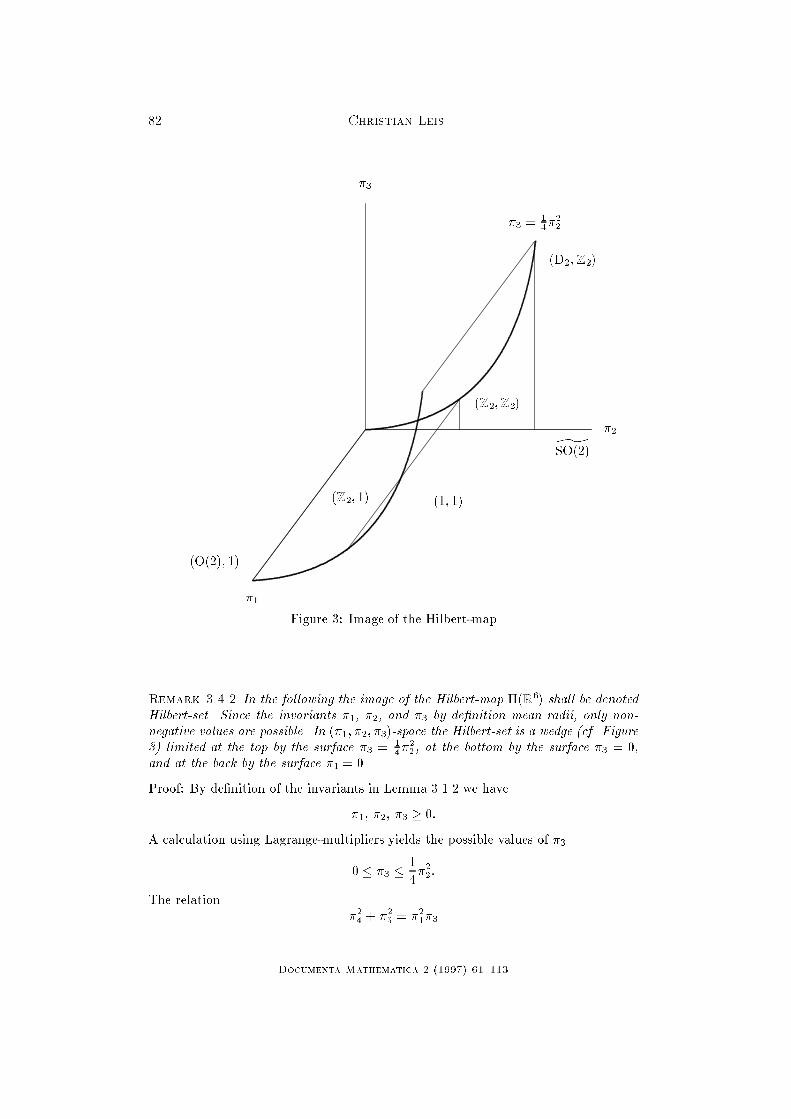
Lemma 3.4.1 The image of the Hilbert-map �(R

6

) is sketched in Figure 3.

One has to imagine circles of radius

�

2

4

+ �

2

5

= �

2

1

�

3

attached to points of the sketch. We have the following assignment

(�

1

; : : : ; �

5

) 2 �(R

6

) isotropy typ

�

1

-axis (O(2); 1)

�

2

-axis

^

SO(2)

�

1

= 0, �

3

=

1

4

�

2

2

(D

2

;Z

2

)

�

1

= 0, 0 < �

3

<

1

4

�

2

2

(Z

2

;Z

2

)

�

1

> 0, �

3

=

1

4

�

2

2

(Z

2

; 1)

�

1

> 0, 0 � �

3

<

1

4

�

2

2

(1; 1):


82 Christian Leis

�

1

�

2

�

3

�

3

=

1

4

�

2

2

(1; 1)

^

SO(2)

(D

2

;Z

2

)

(Z

2

;Z

2

)

(Z

2

; 1)

(O(2); 1)

Figure 3: Image of the Hilbert-map

Remark 3.4.2 In the following the image of the Hilbert-map �(R

6

) shall be denoted

Hilbert-set. Since the invariants �

1

, �

2

, and �

3

by de�nition mean radii, only non-

negative values are possible. In (�

1

; �

2

; �

3

)-space the Hilbert-set is a wedge (cf. Figure

3) limited at the top by the surface �

3

=

1

4

�

2

2

, at the bottom by the surface �

3

= 0,

and at the back by the surface �

1

= 0.

Proof: By de�nition of the invariants in Lemma 3.1.2 we have

�

1

; �

2

; �

3

� 0:

A calculation using Lagrange-multipliers yields the possible values of �

3

0 � �

3

�

1

4

�

2

2

:

The relation

�

2

4

+ �

2

5

= �

2

1

�

3


Invariant Tori 83

has to be satis�ed by Lemma 3.1.2. 1

Remark 3.4.3 Points with isotropy (O(2); 1) and (D

2

;Z

2

) and images of points with

isotropy (T;Z

3

) in the original system (cf. Lemma 3.4.5) under the Hilbert-map

satisfy the relation

� =

1

4

�

2

2

� �

3

= 0:

In the following we shall study the reduced vector �eld (cf. Lemma 3.2.1) on the

Hilbert-set �(R

6

).

Lemma 3.4.4 Let

� =

1

4

�

2

2

� �

3

:

Then

_

� = 4� (�+ �

r

�

1

+

r

�

2

) :

Proof: The stratum

� = 0

corresponds to points with a certain isotropy and, therefore, is �ow invariant. Thus

we have

_

� = 0 for � = 0 and there exists a relation of the form

_

� = � r(�

1

; : : : ; �

5

):

A simple calculation gives the precise relation. 1

Lemma 3.4.5 The orbit space reduction maps Fix (T;Z

3

) to the invariant curve

�

�

1

; �

1

;

1

4

�

2

1

;�

1

2

�

2

1

; 0

�

� �(R

6

); �

1

> 0;

located on the stratum � = 0.

Proof: The proof follows directly from the Lemmata 3.1.2 and 3.3.3. 1

In the following let the parameter of the Hopf-bifurcation � be positive:

� > 0:

We are only interested in supercritical bifurcations.


84 Christian Leis

The restriction of the reduced vector �eld (cf. Lemma 3.2.1) to the statum � = 0 is

_�

1

= 2(�+ �

r

�

1

+ �

r

�

2

)�

1

+ 4

�

(�� )

r

�

4

+ (�� )

i

�

5

�

(3.4.3)

_�

2

= 2(�+ �

r

�

1

+ �

r

�

2

)�

2

+ 4

�

(�� )

r

�

4

� (�� )

i

�

5

�

(3.4.4)

_�

3

=

1

2

�

2

_�

2

(3.4.5)

_�

4

= 2

�

2�+ (�+ �)

r

(�

1

+ �

2

)

�

�

4

+ 2(�� )

i

(��

1

+ �

2

)�

5

+(�� )

r

�

1

�

2

(�

1

+ �

2

) (3.4.6)

_�

5

= 2

�

2�+ (�+ �)

r

(�

1

+ �

2

)

�

�

5

+ 2(�� )

i

(�

1

� �

2

)�

4

+(�� )

i

�

1

�

2

(��

1

+ �

2

): (3.4.7)

Here �

r

; �

r

resp. �

i

; �

i

denote the real resp. imaginary parts of �; �.

Lemma 3.4.6 Let �

r

; �

r

< 0 and �

r

6= �

r

. Then the set of critical points of the

Equations 3.4.3 to 3.4.7 on the stratum � = 0 is given by a curve

g(�

1

) =

�

�

1

; �

2

= �

�

�

1

+

�

�

r

�

;

1

4

�

2

2

;

1

2

�

1

�

2

; 0

�

; 0 � �

1

� �

�

�

r

;

parametrised by �

1

and

h(�

1

) =

�

�

1

; �

1

;

1

4

�

2

1

;�

1

2

�

2

1

; 0

�

; �

1

= �

�

2�

r

:

The curve g(�

1

), 0 � �

1

� �

�

�

r

; connects a critical point with isotropy (O(2); 1),

g

�

�

�

�

r

�

=

�

�

�

�

r

; 0; 0; 0; 0

�

;

with a critical point with isotropy (D

2

;Z

2

),

g(0) =

�

0; �

2

= �

�

�

r

;

1

4

�

2

2

; 0; 0

�

:

The critical point h(�

1

); �

1

= �

�

2�

r

; lies in �(Fix (T;Z

3

)), the image of points with

isotropy (T;Z

3

) in the original system under the Hilbert-map.

Proof: By addition resp. subtraction of Equations 3.4.3 and 3.4.4 one gets the fol-

lowing equations

0 = �(�

1

+ �

2

) + �

r

(�

2

1

+ �

2

2

) + 2�

r

�

1

�

2

+ 4(�� )

r

�

4

; (3.4.8)

0 = �(�

1

� �

2

) + �

r

(�

2

1

� �

2

2

) + 4(�� )

i

�

5

: (3.4.9)

Let (�� )

i

6= 0 then

�

4

= �

�(�

1

+ �

2

) + �

r

(�

2

1

+ �

2

2

) + 2�

r

�

1

�

2

4(�� )

r

;

�

5

= �

�(�

1

� �

2

) + �

r

(�

2

1

� �

2

2

)

4(�� )

i

:


Invariant Tori 85

Inserting this in Equations 3.4.6 and 3.4.7 gives

0 = �

(�

1

+ �

2

)

�

�+ �

r

(�

1

+ �

2

)

��

� + �

r

(�

1

+ �

2

)

�

(�� )

r

;

0 = �

(�

1

� �

2

)

�

�+ �

r

(�

1

+ �

2

)

�

2(�� )

r

(�� )

i

�

2�(�� )

r

+ (�

1

+ �

2

)(�

r2

� �

r2

+ (�� )

i2

�

: (3.4.10)

Looking for nontrivial critical points, one, therefore, has to study two cases.

Let �

1

+ �

2

= �

�

�

r

. Since we assume � > 0, only the choice �

r

< 0 gives solutions

that lie in �(R

6

). By insertion one gets the curve

g(�

1

) =

�

�

1

; �

2

= �

�

�

1

+

�

�

r

�

;

1

4

�

2

2

;

1

2

�

1

�

2

; 0

�

; 0 � �

1

� �

�

�

r

;

of critical points. Lemma 3.4.1 gives the associated orbit types.

Now let �

1

+ �

2

= �

�

�

r

. Only the choice �

r

< 0 gives solutions that lie in �(R

6

) as

above. By insertion in Equation 3.4.10 one gets the condition

0 =

�

(�� )

r2

+ (� � �)

i2

�

�

2

(�+ 2�

r

�

2

)

2�

r3

(�� )

i

:

In order to get critical points, one has to choose

�

1

= �

2

= �

�

2�

r

:

By insertion one obtains the critical point

h(�

1

) =

�

�

1

; �

1

;

1

4

�

2

1

;�

1

2

�

2

1

; 0

�

; �

1

= �

�

2�

r

;

lying in �(Fix (T;Z

3

)) (cf. Lemma 3.4.5). It shall be shown that there are no other

critical points with radius

�

1

+ �

2

= �

�

�

r

:

Therefore the group orbit of periodic orbits with isotropy (T;Z

3

) in the original system

can only intersect the strati�ed space in the curve given in Lemma 3.4.5.

Now let (�� )

i

= 0. Equations 3.4.8 and 3.4.9 yield

0 = �(�

1

+ �

2

) + �

r

(�

2

1

+ �

2

2

) + 2�

r

�

1

�

2

+ 4(�� )

r

�

4

;

0 = (�

1

� �

2

)

�

� + �

r

(�

1

+ �

2

)

�

:

Consequently we have to study two cases.

Let �

1

= �

2

. Then

�

4

= �

�

�+ (�+ �)

r

�

1

�

�

1

2(�� )

r

:


86 Christian Leis

By insertion in Equation 3.4.6 one gets

0 = �

�

1

(� + 2�

r

�

1

)(� + 2�

r

�

1

)

(�� )

r

:

The choice �

1

= �

2

= �

�

2�

r

and the relation

�

2

4

+ �

2

5

= �

2

1

�

3

=

1

4

�

4

1

give the critical point

�

�

1

; �

1

;

1

4

�

2

1

;

1

2

�

2

1

; 0

�

; �

1

= �

�

2�

r

;

that lies on the curve g(�

1

).

The case �

1

= �

2

= �

�

2�

r

again yields the solution h(�

1

); �

1

= �

�

2�

r

:

Finally we have to study the case �

1

+ �

2

= �

�

�

r

. We get

�

4

= �

�

1

2�

r

(�+ �

r

�

1

)

=

1

2

�

1

�

2

:

The relation

�

2

4

+ �

2

5

=

1

4

�

2

1

�

2

2

yields �

5

= 0. So again we get the curve g(�

1

). 1

Lemma 3.4.7

�(Fix (T;Z

3

)) \ g(�

1

) = ;; 0 � �

1

� �

�

�

r

:

The critical point h(�

1

), �

1

= �

�

2�

r

, (cf. Lemma 3.4.6) that lies in �(Fix(T;Z

3

)) is

isolated in the Hilbert-set �(R

6

).

Proof: For points lying on the curve g(�

1

) we have �

1

+ �

2

= �

�

�

r

. Points in

�(Fix (T;Z

3

)) satisfy the condition �

1

= �

2

(cf. Lemma 3.4.5). For a potential

intersection this means �

1

= �

2

= �

�

2�

r

. We have

g

�

�

�

2�

r

�

=

�

�

�

2�

r

;�

�

2�

r

;

1

16

�

2

�

r2

;+

1

8

�

2

�

r2

; 0

�

whereas

�(Fix (T;Z

3

)) \

�

�

1

= �

�

2�

r

�

=

�

�

�

2�

r

;�

�

2�

r

;

1

16

�

2

�

r2

;�

1

8

�

2

�

r2

; 0

�

:

On the stratum � = 0 the critical point h(�

1

), �

1

= �

�

2�

r

, (cf. Lemma 3.4.6) that

lies on �(Fix(T;Z

3

)), therefore, is isolated. We shall show in Lemma 3.4.8 that

there are no further critical points in the Hilbert-set in the region � 6= 0 near h(�

1

),

�

1

= �

�

2�

r

. 1


Invariant Tori 87

Now we are looking for critical points of the reduced vector �eld (cf. Lemma 3.2.1)

in �(R

6

) that do not lie on the stratum � = 0. Such a critical point has to meet the

condition (cf. Lemma 3.4.4)

_

� = 4� (�+ �

r

�

1

+

r

�

2

) = 0:

Since we assumed � 6= 0, this means

�+ �

r

�

1

+

r

�

2

= 0: (3.4.11)

So we get the following equations:

0 = 2(�+ �

r

�

1

+ �

r

�

2

)�

1

+ 4

�

(�� )

r

�

4

+ (�� )

i

�

5

�

(3.4.12)

0 = 8(�� )

r

�

3

+ 4

�

(�� )

r

�

4

� (�� )

i

�

5

�

(3.4.13)

0 =

1

2

�

2

_�

2

(3.4.14)

0 = 2

�

2� + (�+ �)

r

(�

1

+ �

2

)

�

�

4

+ 2(�� )

i

(��

1

+ �

2

)�

5

+(�� )

r

�

1

(�

1

�

2

+ 4�

3

) (3.4.15)

0 = 2

�

2� + (�+ �)

r

(�

1

+ �

2

)

�

�

5

+ 2(�� )

i

(�

1

� �

2

)�

4

+(�� )

i

�

1

(��

1

�

2

+ 4�

3

) (3.4.16)

�

2

= �

� + �

r

�

1

r

: (3.4.17)

Here �

r

; �

r

;

r

resp. �

i

; �

i

again denote the real resp. imaginary parts of �; �; .

In the following we shall assume

�

r

< �

r

<

r

< 0:

In Lemma 3.5.1 we shall show that only for this choice of the coe�cients the solutions

with isotropy (O(2); 1) resp.

^

SO(2) can be stable simultaneously. Investigations using

the topological Conlex-index suggested to study this case. In the following lemma

the solution with isotropy

^

SO(2) is being described.

Lemma 3.4.8 Let �

r

< �

r

<

r

< 0. Then

�

0;�

�

r

; 0; 0; 0

�

is the only critical point of the reduced vector �eld in �(R

6

) with � 6= 0. This solution

has isotropy

^

SO(2).

Proof: First let (�� )

i

6= 0. By addition resp. subtraction of Equations 3.4.12 and

3.4.13 we get

0 = (� + �

r

�

1

+ �

r

�

2

)�

1

+ 4(�� )

r

�

4

+ 4(�� )

r

�

3

;

0 = (� + �

r

�

1

+ �

r

�

2

)�

1

+ 4(�� )

i

�

5

� 4(�� )

r

�

3

:


88 Christian Leis

Therefore we have

�

4

= �

(� + �

r

�

1

+ �

r

�

2

)�

1

+ 4(�� )

r

�

3

4(�� )

r

;

�

5

= �

(� + �

r

�

1

+ �

r

�

2

)�

1

� 4(�� )

r

�

3

4(�� )

i

:

Insertion in Equation 3.4.15 yields

(� � )

r

�

�(� � )

r

+ �

r

�

1

(� � )

r

�

(��

1

� �

r

�

2

1

+ 4

r

�

3

)

(�� )

r

r2

= 0:

Let

�

1

= �

�(�� )

r

�

r

(� � )

r

> 0:

Using Equation 3.4.17 we get

�

2

=

�(�� )

r

�

r

(� � )

r

> 0:

Together with Equation 3.4.16 this yields

0 =

(�� )

r

�

(�� )

r2

+ (�� )

i2

�

�

�

� �

2

(�� )

r2

+ 4�

r2

�

3

(� � )

r2

�

2�

r3

(�� )

r

(�� )

i

(� � )

r2

:

So we have

�

3

=

�

2

(� � �)

r2

4�

r2

(� � )

r2

=

1

4

�

2

2

:

This solution lies on the stratum � = 0.

Now let

�

3

=

�

1

(� + �

r

�

1

)

4

r

= �

1

4

�

1

�

2

:


0 = �2(�� )

i2

�

2

1

�

2

�

(�� )

i2

�

1

�

�+ (� + )

r

�

1

�

2

2

r2

�

�

1

�

�(� + � � 2 )

r

+ �

1

(�+ �)

r

(� � )

r

�

2

2

r2

:

Since all elements of the sum are nonpositive in �(R

6

) the sum can only be zero if all

elements are zero. This is only possible if �

1

= 0. This yields

�

0;�

�

r

; 0; 0; 0

�

;

the solution with isotropy

^

SO(2).


Invariant Tori 89

Second let (� � �)

i

= 0. Again by addition resp. subtraction of the Equations

3.4.12 and 3.4.13 we get

�

3

=

(�+ �

r

�

1

+ �

r

�

2

)�

1

4(�� )

r

;

�

4

= �

2(�� )

r

�

3

(�� )

r

: (3.4.18)

Furthermore we have

�

2

= �

� + �

r

�

1

r

:


0 =

�

2�+ (�+ �)

r

(�

1

+ �

2

)

�

�

5

:

In order to solve this equation, we have to look at several cases.

Let �

5

= 0. Then

�

2

4

+ �

2

5

= �

2

1

�

3

and Equation 3.4.18 yields

4(�� )

r2

(�� )

r2

�

2

3

= �

2

1

�

3

:

For �

3

6= 0 we get

�

1

= �

�(�� )

r

�

r

(� � )

r

> 0; �

2

=

�(�� )

r

�

r

(� � )

r

> 0; �

3

=

1

4

�

2

2

:

Therefore the solution lies on the stratum � = 0.

The choice �

3

= 0 and Equation 3.4.16 yield the solution

�

0;�

�

r

; 0; 0; 0

�

with isotropy

^

SO(2). For �

5

6= 0 and

0 = 2�+ (�+ �)

r

(�

1

+ �

2

)

Equation 3.4.15 gives

0 = �

1

(�

1

�

2

+ 4�

3

):

Choosing �

1

= 0 again yields the solution with isotropy

^

SO(2).

For �

1

6= 0 one gets the solution

�

1

= �

�(�+ � � 2 )

r

(�+ �)

r

(� � )

r

> 0;

�

2

=

�(� � �)

r

(�+ �)

r

(� � )

r

> 0;

�

3

=

�

2

(�� )

r

(�+ � � 2 )

r

4(�+ �)

r2

(� � )

r2

< 0

that does not lie in �(R

6

). 1


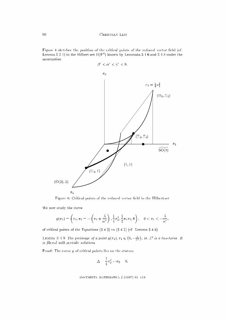
90 Christian Leis

Figure 4 sketches the position of the critical points of the reduced vector �eld (cf.

Lemma 3.2.1) in the Hilbert-set �(R

6

) known by Lemmata 3.4.6 and 3.4.8 under the

assumption

�

r

< �

r

<

r

< 0:

�

1

�

2

�

3

�

3

=

1

4

�

2

2

(1; 1)

^

SO(2)

(D

2

;Z

2

)

(Z

2

;Z

2

)

(Z

2

; 1)

(O(2); 1)

u

u

u

u

Figure 4: Critical points of the reduced vector �eld in the Hilbert-set

We now study the curve

g(�

1

) =

�

�

1

; �

2

= �

�

�

1

+

�

�

r

�

;

1

4

�

2

2

;

1

2

�

1

�

2

; 0

�

; 0 < �

1

< �

�

�

r

;

of critical points of the Equations (3.4.3) to (3.4.7) (cf. Lemma 3.4.6).

Lemma 3.4.9 The preimage of a point g(�

1

); �

1

2

�

0;�

�

�

r

�

, in R

6

is a two-torus. It

is �bered with periodic solutions.

Proof: The curve g of critical points lies on the statum

� =

1

4

�

2

2

� �

3

= 0:


Invariant Tori 91

Introducing polar coordinates in the form

z

j

= r

j

e

i�

j

; j 2 f�2; 0; 2g;

yields

r

�2

= r

2

:

The choice of

�

1

= r

2

0

2

�

0;�

�

�

r

�

and the condition

�

1

+ �

2

= �

�

�

r

determine the radii. Let

� = 2�

0

� �

�2

� �

2

:

Then the conditions for �

4

resp. �

5

yield, in polar coordinates, the phase relations

cos � = 1; sin � = 0

and, thus,

� = 0 mod2�:

So one angle is determined, two are still available, the preimage is a 2-torus. Points

on the surface � = 0 have the (conjugated) isotropy (Z

2

; 1). Therefore it is possible

just to look at points of the form (z

2

; z

0

; z

2

) in order to determine the resulting �ow

on the preimage of a point on the curve of �xed points. Thus we have the additional

condition

�

�2

= �

2

:

Using � = 0mod2�, one sees that

�

0

= �

2

mod�:

Inserting this into the di�erential equation yields

_

�

0

= !

0

= ! + �

i

�

r

2

0

+ 2r

2

2

�

:

Thus the 2�torus is �bered with periodic solutions of period near

2�

!

. 1

3.5 Stability of the critical points of the reduced vector field

In Lemmata 3.4.6 and 3.4.8 we have shown that in the case of supercritical bifurcation

(� > 0) the coe�cients �

r

; �

r

;

r

have to be negative in order that the corresponding

solutions lie in the image of the Hilbert-map �(R

6

). The following lemma gives a

condition on the choice of the coe�cients relative to each other.


92 Christian Leis

Lemma 3.5.1 Only by choosing the coe�cients

�

r

< �

r

<

r

< 0; �

r

2

�

1

4

(� + 3 )

r

;

r

�

;

the critical points with isotropy (O(2); 1) resp.

^

SO(2) of the reduced vector �eld (cf.

Lemma 3.2.1) can be stable simultaneously. The stability of the solution with isotropy

(O(2); 1) is determined by higher order terms because of the existence of a curve of

critical points (cf. Lemma 3.4.6).

Proof: The calculations of [IoRo] yield (using our parameters) up to third order the

following conditions for the stability of the periodic solutions with isotropy (O(2); 1)

resp.

^

SO(2) in the original, ten dimensional system:

isotropy nontrivial Floquet-exponents

(O(2); 1) �2� < 0;�

2�

�

r

(�� )

r

< 0;�

2�

�

r

(�4�+ � + 3 )

r

< 0

^

SO(2) �2� < 0;�

2�

r

(�� ); cc;

�

r

( � �); cc;

3�

2

r

( � �); cc:

Here cc denotes the complex conjugate of the preceding number.

So we get the conditions

�

r

< �

r

<

r

< 0

and

�

r

+ 3

r

< 4�

r

:

The ansatz

�

r

= t �

r

+ (1� t)

r

; t 2 (0; 1);

yields

(� � )

r

(1� 4t) < 0

and, therefore, we have

t 2

�

0;

1

4

�

:

This means

�

r

2

�

1

4

(� + 3 )

r

;

r

�

:

Especially

(�� )

r

(� � )

r

2

�

0;

1

4

�

: 1


Invariant Tori 93

Now we want to determine the linearization of the reduced vector �eld (cf. Lemma

3.2.1) along the curve g(�

1

) of critical points (cf. Lemma 3.4.6). For the general

linearization L one gets

L =

0

B

B

B

B

@

2�+ 4�

1

�

r

+ 2�

2

�

r

2�

2

�

r

4�

3

�

r

2�

4

(�+ �)

r

� 2�

5

(�� )

i

+ (2�

1

�

2

+ 4�

3

)(�� )

r

2�

5

(�+ �)

r

+ 2�

4

(�� )

i

+ (�2�

1

�

2

+ 4�

3

)(�� )

i

2�

1

�

r

2� + 2�

1

�

r

+ 4�

2

r

4�

3

�

r

+ 2

�

�

4

(�� )

r

� �

5

(�� )

i

�

2�

4

(�+ �)

r

+ 2�

5

(�� )

i

+ �

2

1

(�� )

r

2�

5

(�+ �)

r

� 2�

4

(�� )

i

� �

2

1

(�� )

i

0 4(�� )

r

4(�� )

i

8(�� )

r

4(�� )

r

�4(�� )

i

4(�+ �

r

�

1

+ �

r

�

2

) 2�

2

(�� )

r

�2�

2

(�� )

i

4�

1

(�� )

r

4�+ 2(�

1

+ �

2

)(�+ �)

r

2(��

1

+ �

2

)(�� )

i

4�

1

(�� )

i

2(�

1

� �

2

)(�� )

i

4�+ 2(�

1

+ �

2

)(�+ �)

r

1

C

C

C

C

A

:

We are interested in the eigenvalues of L along the curve g(�

1

) with reference to

�(R

6

) � R

5

. Thus we have to determine the tangent space at points of the curve in

�(R

6

). It is given by the relation

�

2

4

+ �

2

5

= �

2

1

�

3

:

The curve itself lies on the stratum

� =

1

4

�

2

2

� �

3

= 0:

So we get the following lemma.

Lemma 3.5.2 The tangent space at the stratum � = 0 along the curve

g(�

1

); 0 < �

1

< �

�

�

r

;

is spanned by the vectors

t

1

=

�

1;�1;�

1

2

�

2

;

1

2

(�

2

� �

1

); 0

�

;

t

2

=

�

�

1

; �

2

;

1

2

�

2

2

; �

1

�

2

; 0

�

;

t

3

=

�

2�

r

(� � �)

i

;�2�

r

(�� )

i

;��

2

�

r

(�� )

i

; �

r

(�

2

� �

1

)(�� )

i

;

��

r

(�

1

+ �

2

)(� � �)

r

) :

The vectors t

1

; t

2

; t

3

are eigenvectors of L to the eigenvalues

ew

1

= 0;

ew

2

= �2� = 2�

r

(�

1

+ �

2

);

ew

3

=

2(�� )

r

�

�

r

= �2(� � �)

r

(�

1

+ �

2

):


94 Christian Leis

The curve g(�

1

); 0 < �

1

< �

�

�

r

; is stable on the stratum � = 0.

Proof: The relations �

2

4

+ �

2

5

= �

2

1

�

3

and � = 0 yield the following vectors normal to

the tangent space at the surface � = 0 in �(R

6

) � R

5

:

n

1

=

�

�2�

1

�

3

; 0;��

2

1

; 2�

4

; 2�

5

�

;

n

2

=

�

0;

1

2

�

2

;�1; 0; 0

�

:

The orthogonal complement to Span(n

1

; n

2

) is spanned by the vectors t

1

; t

2

; t

3

. A

simple calculation shows that these vectors are eigenvectors to the given eigenvalues.

The eigenvector t

1

points along the curve of critical points. Therefore the associated

eigenvalue is zero. By de�nition of the curve g(�

1

) we have

�

1

+ �

2

= �

�

�

r

:

Therefore the curve g(�

1

); 0 < �

1

< �

�

�

r

; is stable on the stratum � = 0. 1

Now we want to determine the linearization of the reduced vector �eld along the

curve g(�

1

) of �xed points in the direction of the principal stratum. We shall show

that there exists a point ~�

1

on the curve g(�

1

) in which the stability of the curve

changes from stable to unstable in the direction of the principal stratum. In this

point the linearization L of the vector �eld of the reduced equation has a nontrivial

two dimensional Jordan-block with respect to the eigenvalue zero.

Let

t = (0; 1; 0; 0;0):

Then n

1

t = 0 and n

2

t 6= 0 for �

2

6= 0. Thus the vectors t

1

; t

2

; t

3

; t span the tangent

space at the Hilbert-set �(R

6

) along the curve g(�

1

); 0 < �

1

< �

�

�

r

: One gets

L t = a t

1

+ b t

2

+ c t

3

+ d t

with

a = �2�

1

(�� )

r2

+ (�� )

i2

(�� )

r

;

b = 2�

r

;

c = �

1

(�� )

i

�

r

(�� )

r

;

d = 4

�(�� )

r

+ �

1

�

r

(� � )

r

�

r

:

Restricted to the tangent space at the curve g(�

1

); 0 < �

1

< �

�

�

r

; according to our

choice of the vectors t

1

; t

2

; t

3

; t, L has the form

~

L:

~

L =

0

B

B

@

0 0 0 a

0 �2� 0 b

0 0

2(��)

r

�

�

r

c

0 0 0 d

1

C

C

A

:


Invariant Tori 95

Especially the fourth eigenvalue is

ew

4

= d

= 4

�(�� )

r

+ �

1

�

r

(� � )

r

�

r

= �4

�

�

1

(�� )

r

+ �

2

(�� )

r

�

:

For

~�

1

= �

�(�� )

r

�

r

(� � )

r

we have ew

4

(~�

1

) = 0: Choosing the coe�cients according to Lemma 3.5.1 yields

0 < ~�

1

< �

�

4�

r

:

The point g(~�

1

) is exactly the intersection point of the curve g(�

1

); 0 � �

1

� �

�

�

r

;

with the surface �+ �

r

�

1

+

r

�

2

= 0 (cf. Lemma 3.4.4). Only on this surface we can

have critical points of the reduced vector �eld (cf. Lemma 3.2.1) outside the stratum

� = 0 (cf. Lemma 3.4.6).

For

h(~�

1

) =

0

B

B

B

B

B

B

B

B

B

B

B

B

B

B

B

@

�

(�� )

r

�

�

(��)

r2

�(��)

i2

�

(��)

r2

(�� )

r

(�� )

r

�

�

(��)

r2

�(��)

i2

�

(��)

r2

(�� )

r

�

2

�

(��)

r3

�(�� )

r

(��)

i2

�

2�

r

(��)

r

(�� )

r2

�

(�� )

r

�

2

�

2(��)

r3

+(�2�+�+ )

r

(��)

i2

�

2�

r

(��)

r2

(�� )

r2

(�� )

r

(��)

i

�

2

2�

r

(��)

r

(�� )

r

1

C

C

C

C

C

C

C

C

C

C

C

C

C

C

C

A

we have

h(~�

1

) = �

r

t

2

(~�

1

)�

(�� )

i

~�

1

2(�� )

r2

t

3

(~�

1

) + �t:

Consequently, h(~�

1

) 2 Span

�

t

1

(~�

1

); t

2

(~�

1

); t

3

(~�

1

); t

�

; and one sees that Lh(~�

1

) =

j t

1

(~�

1

) with

j =

2�

2

(�� )

r

�

(�� )

r2

+ (�� )

i2

�

�

r

(�� )

r

(� � )

r

< 0:

So we have shown the following lemma.

Lemma 3.5.3 In the point g(~�

1

), ~�

1

= �

�(�� )

r

�

r

(�� )

r

, the linearization L of the vector

�eld of the reduced equation (cf. Lemma 3.2.1) has a nontrivial, two dimensional

Jordan-block with respect to the eigenvalue zero.

Up to now we have studied the reduced vector �eld resulting from the normal

form up to third order (cf. [IoRo]). It has been shown in this section that this vector

�eld is degenerate. In the next section we shall use �fth order terms to investigate

this degeneracy.


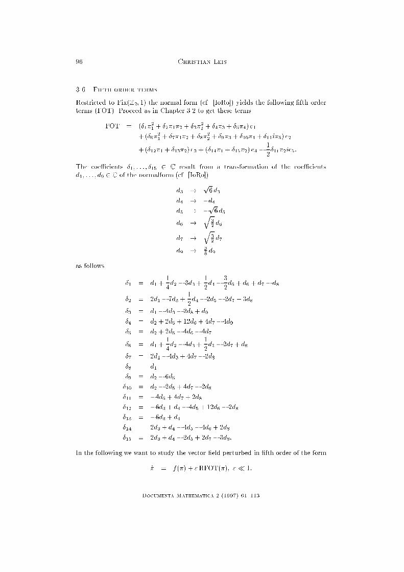
96 Christian Leis

3.6 Fifth order terms

Restricted to Fix(Z

2

; 1) the normal form (cf. [IoRo]) yields the following �fth order

terms (FOT). Proceed as in Chapter 3.2 to get these terms.

FOT = (�

1

�

2

1

+ �

2

�

1

�

2

+ �

3

�

2

2

+ �

4

�

3

+ �

5

�

4

) e

1

+(�

6

�

2

1

+ �

7

�

1

�

2

+ �

8

�

2

2

+ �

9

�

3

+ �

10

�

4

+ �

11

i�

5

) e

2

+(�

12

�

1

+ �

13

�

2

) e

3

+ (�

14

�

1

+ �

15

�

2

) e

4

�

1

2

�

11

�

2

ie

5

:

The coe�cients �

1

; : : : ; �

15

2 C result from a transformation of the coe�cients

d

1

; : : : ; d

9

2 C of the normalform (cf. [IoRo])

d

3

!

p

6d

3

d

4

! �d

4

d

5

! �

p

6 d

5

d

6

!

q

3

2

d

6

d

7

!

q

3

2

d

7

d

9

!

3

8

d

9

as follows

�

1

= d

1

+

1

4

d

2

� 3d

3

+

1

2

d

4

�

3

2

d

5

+ d

6

+ d

7

� d

8

�

2

= 2d

1

� 7d

3

+

1

2

d

4

� 2d

5

� 2d

7

+ 3d

8

�

3

= d

1

� 4d

3

� 2d

8

+ d

9

�

4

= d

2

+ 2d

5

+ 12d

6

+ 4d

7

� 4d

9

�

5

= d

2

+ 2d

5

� 4d

6

� 4d

7

�

6

= d

1

+

1

4

d

2

� 4d

3

+

1

2

d

5

� 2d

7

+ d

8

�

7

= 2d

1

� 4d

3

+ 4d

7

� 2d

8

�

8

= d

1

�

9

= d

2

� 6d

5

�

10

= d

2

� 2d

5

+ 4d

7

� 2d

8

�

11

= �4d

5

+ 4d

7

+ 2d

8

�

12

= �6d

3

+ d

4

� 4d

5

+ 12d

6

� 2d

8

�

13

= �6d

3

+ d

4

�

14

= 2d

3

+ d

4

� 4d

5

� 4d

6

+ 2d

8

�

15

= 2d

3

+ d

4

� 2d

5

+ 2d

7

� 3d

8

:

In the following we want to study the vector �eld perturbed in �fth order of the form

_� = f(�) + "RFOT(�); "� 1:


Invariant Tori 97

By reduction of the �fth order terms (FOT) to the orbit space one gets the pertur-

bation RFOT (reduced �fth order terms) with components RFOT1; : : : ;RFOT5.

RFOT1 = 2�

1

(�

r

1

�

2

1

+ �

r

2

�

1

�

2

+ �

r

3

�

2

2

+ �

r

4

�

3

) + �

4

�

2(�

5

+ �

14

)

r

�

1

+(�

11

+ 2�

15

)

r

�

2

�

+ �

5

�

2�

i

14

�

1

+ (�

11

+ 2�

15

)

i

�

2

�

RFOT2 = 4�

r

12

�

1

�

3

+ 2�

2

�

�

r

6

�

2

1

+ �

r

7

�

1

�

2

+ �

r

8

�

2

2

+ (�

9

+ 2�

13

)

r

�

3

�

+�

4

�

2�

r

14

�

1

+ (2�

10

� �

11

+ 2�

15

)

r

�

2

�

� �

5

�

2�

i

14

�

1

+(�

11

+ 2�

15

)

i

�

2

�

RFOT3 = 2�

3

�

2�

r

6

�

2

1

+ (2�

7

+ �

12

)

r

�

1

�

2

+ (2�

8

+ �

13

)

r

�

2

2

+ 2�

r

9

�

3

�

+�

4

�

�

2

�

�

r

14

�

1

�

�

1

2

�

11

� �

15

�

r

�

2

�

+ 4�

r

10

�

3

�

��

5

�

2

�

i

14

�

1

�

�

1

2

�

11

� �

15

�

i

�

2

!

+ 4�

i

11

�

3

!

RFOT4 = 2�

4

�

(�

1

+ �

6

)

r

�

2

1

+

�

�

2

+ �

7

+

1

2

�

12

�

r

�

1

�

2

+

�

�

3

+ �

8

+

1

2

�

13

�

r

�

2

2

+ (�

4

+ �

9

)

r

�

3

+ (�

5

+ �

10

)

r

�

4

�

�2�

5

�

(�

1

� �

6

)

i

�

2

1

+

�

�

2

� �

7

�

1

2

�

12

�

i

�

1

�

2

+

�

�

3

� �

8

�

1

2

�

13

�

i

�

2

2

+ (�

4

� �

9

)

i

�

3

� �

r

11

�

5

�

�2�

4

�

5

(�

5

� �

10

+ �

11

)

i

+ �

1

�

1

2

�

r

14

�

2

1

�

2

�

�

1

4

�

11

�

1

2

�

15

�

r

�

1

�

2

2

+2�

r

14

�

1

�

3

+ (�

11

+ 2�

15

)

r

�

2

�

3

�

RFOT5 = 2�

4

�

(�

1

� �

6

)

i

�

2

1

+

�

�

2

� �

7

�

1

2

�

12

�

i

�

1

�

2

+

�

�

3

� �

8

�

1

2

�

13

�

i

�

2

2

+(�

4

� �

9

)

i

�

3

+ (�

5

� �

10

)

i

�

4

�

+2�

5

�

(�

1

+ �

6

)

r

�

2

1

+

�

�

2

+ �

7

+

1

2

�

12

�

r

�

1

�

2

+

�

�

3

+ �

8

+

1

2

�

13

�

r

�

2

2

+ (�

4

+ �

9

)

r

�

3

� �

i

11

�

5

�

+2�

4

�

5

(�

5

+ �

10

� �

11

)

r

+ �

1

�

�

1

2

�

i

14

�

2

1

�

2

+

�

1

4

�

11

�

1

2

�

15

�

i

�

1

�

2

2

+2�

i

14

�

1

�

3

+ (�

11

+ 2�

15

)

i

�

2

�

3

�

:


98 Christian Leis

Lemma 3.6.1 Restriction to the stratum � = 0 yields

�RFOT1 = 2�

1

�

�

r

1

�

2

1

+ �

r

2

�

1

�

2

+

�

�

3

+

1

4

�

4

�

r

�

2

2

�

+�

4

�

2(�

5

+ �

14

)

r

�

1

+ (�

11

+ 2�

15

)

r

�

2

�

+�

5

�

2�

i

14

�

1

+ (�

11

+ 2�

15

)

i

�

2

�

�RFOT2 = 2�

2

�

�

r

6

�

2

1

+

�

�

7

+

1

2

�

12

�

r

�

1

�

2

+

�

�

8

+

1

4

�

9

+

1

2

�

13

�

r

�

2

2

�

+�

4

�

2�

r

14

�

1

+ (2�

10

� �

11

+ 2�

15

)

r

�

2

�

��

5

�

2�

i

14

�

1

+ (�

11

+ 2�

15

)

i

�

2

�

�RFOT3 =

1

2

�

2

�RFOT2

�RFOT4 = 2�

4

�

(�

1

+ �

6

)

r

�

2

1

+

�

�

2

+ �

7

+

1

2

�

12

�

r

�

1

�

2

+

�

�

3

+

1

4

�

4

+ �

8

+

1

4

�

9

+

1

2

�

13

�

r

�

2

2

+ (�

5

+ �

10

)

r

�

4

�

�2�

5

�

(�

1

� �

6

)

i

�

2

1

+

�

�

2

� �

7

�

1

2

�

12

�

i

�

1

�

2

+

�

�

3

+

1

4

�

4

� �

8

�

1

4

�

9

�

1

2

�

13

�

i

�

2

2

� �

r

11

�

5

�

�2�

4

�

5

(�

5

� �

10

+ �

11

)

i

+ �

1

�

2

�

1

2

�

r

14

�

2

1

�

�

1

4

�

11

�

1

2

�

14

�

1

2

�

15

�

r

�

1

�

2

+

�

1

4

�

11

+

1

2

�

15

�

r

�

2

2

�

�RFOT5 = 2�

4

�

(�

1

� �

6

)

i

�

2

1

+

�

�

2

� �

7

�

1

2

�

12

�

i

�

1

�

2

+

�

�

3

+

1

4

�

4

� �

8

�

1

4

�

9

�

1

2

�

13

�

i

�

2

2

+ (�

5

� �

10

)

i

�

4

�

+2�

5

�

(�

1

+ �

6

)

r

�

2

1

+

�

�

2

+ �

7

+

1

2

�

12

�

r

�

1

�

2

+

�

�

3

+

1

4

�

4

+ �

8

+

1

4

�

9

+

1

2

�

13

�

r

�

2

2

� �

i

11

�

5

�

+2�

4

�

5

(�

5

+ �

10

� �

11

)

r

+ �

1

�

2

�

�

1

2

�

i

14

�

2

1

+

�

1

4

�

11

+

1

2

�

14

�

1

2

�

15

�

i

�

1

�

2

+

�

1

4

�

11

+

1

2

�

15

�

i

�

2

2

�

:

Here �RFOT1, : : : , �RFOT5 denote the components of the reduced �fth order terms

(RFOT) restricted to the statum � = 0.


Invariant Tori 99

3.7 Singular perturbation theory

For the moment we want to restrict our considerations to the stratum � = 0. The

curve g(�

1

); 0 � �

1

� �

�

�

r

; of critical points of the reduced vector �eld _� = f(�) (cf.

Equations 3.4.3 to 3.4.7) is located on this stratum (cf. Lemma 3.4.6). According to

Lemma 3.5.2 this curve is asymptotically stable for our choice of the coe�cients

�

r

< �

r

<

r

< 0:

Now we want to study the perturbed vector �eld (cf. Lemma 3.6.1)

_� = f

"

(�) = f(�) + "�RFOT(�); "� 1: (3.7.19)

We have the following propostion.

Proposition 3.7.1 For the perturbed Vector Field 3.7.19 and 0 < j"j < "

0

there per-

sists an invariant curve g

"

near g on the stratum � = 0. This curve g

"

is parametrised

over �

1

. The vector �eld on g

"

has the form

r(�

1

) = 2

�

1

�

2

�

1

+ �

2

�

16�

2

1

+ 16

�

�

r

�

1

+ 3

�

2

�

r2

�

d

with

0 < �

1

< �

�

�

r

; �

1

+ �

2

= �

�

�

r

;

d =

�

(d

6

+ d

7

� d

8

)

r

+

(�� )

i

(�� )

r

(d

6

+ d

7

� d

8

)

i

�

:

Proof: In Lemma 3.5.2 we showed that the curve g(�

1

); 0 < �

1

< �

�

�

r

, is normally

hyperbolic. Thus an invariant curve g

"

near g persists under small perturbations.

The curve g

"

will no longer consist of critical points but there will be a resulting �ow

on g

"

. This �ow is determined in the lowest order by projection of the perturbation

onto the curve g.

Let

E =

�

g(�

1

) j 0 < �

1

< �

�

�

r

�

be the curve of critical points of the vector �eld f

0

(�) on the stratum

F =

�

� 2 �(R

6

) j�(�) = 0

:

For a point � 2 E let

Tf

0

(�) : T

�

F ! T

�

F

denote the linearization of f

0

in �. By construcion T

�

E lies in the kernel of Tf

0

(�).

So a linear map

Qf

0

(�) :

T

�

F

T

�

E

!

T

�

F

T

�

E


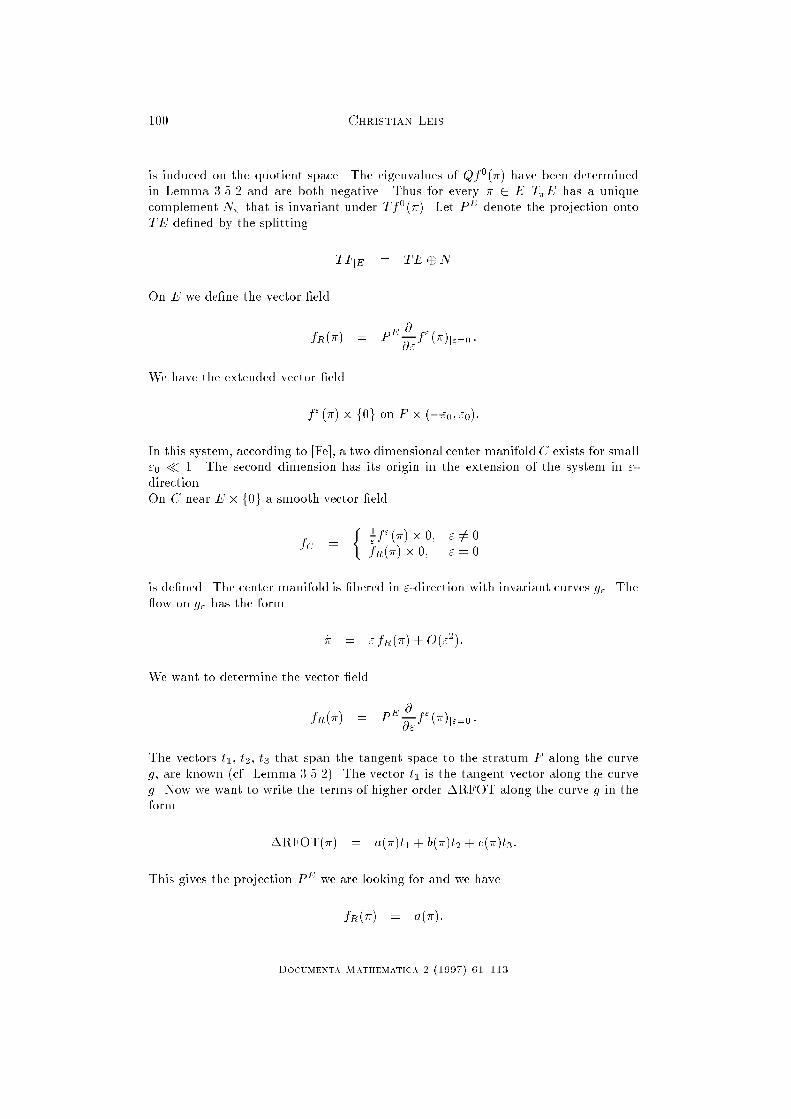
100 Christian Leis

is induced on the quotient space. The eigenvalues of Qf

0

(�) have been determined

in Lemma 3.5.2 and are both negative. Thus for every � 2 E T

�

E has a unique

complement N

�

that is invariant under Tf

0

(�). Let P

E

denote the projection onto

TE de�ned by the splitting

TF

jE

= TE �N

On E we de�ne the vector �eld

f

R

(�) = P

E

@

@"

f

"

(�)

j"=0

:

We have the extended vector �eld

f

"

(�)� f0g on F � (�"

0

; "

0

):

In this system, according to [Fe], a two dimensional center manifoldC exists for small

"

0

� 1. The second dimension has its origin in the extension of the system in "-

direction.

On C near E � f0g a smooth vector �eld

f

C

=

�

1

"

f

"

(�)� 0; " 6= 0

f

R

(�) � 0; " = 0

is de�ned. The center manifold is �bered in "-direction with invariant curves g

"

. The

�ow on g

"

has the form

_� = " f

R

(�) + O("

2

):

We want to determine the vector �eld

f

R

(�) = P

E

@

@"

f

"

(�)

j"=0

:

The vectors t

1

; t

2

; t

3

that span the tangent space to the stratum F along the curve

g, are known (cf. Lemma 3.5.2). The vector t

1

is the tangent vector along the curve

g. Now we want to write the terms of higher order �RFOT along the curve g in the

form

�RFOT(�) = a(�)t

1

+ b(�)t

2

+ c(�)t

3

:

This gives the projection P

E

we are looking for and we have

f

R

(�) = a(�):


Invariant Tori 101

As the restriction of the vector �eld

@

@"

f

"

(�)

j"=0

along the curve g one gets

r

1

= �

1

�

2�

r

1

�

2

1

+ (2�

2

+ �

5

+ �

14

)

r

�

1

�

2

+

�

2�

3

+

1

2

�

4

+

1

2

�

11

+ �

15

�

r

�

2

2

�

r

2

= �

2

�

(2�

6

+ �

14

)

r

�

2

1

+

�

2�

7

+ �

10

�

1

2

�

11

+ �

12

+ �

15

�

r

�

1

�

2

+

�

2�

8

+

1

2

�

9

+ �

13

�

r

�

2

2

�

r

3

=

1

2

�

2

r

2

r

4

= �

1

�

2

��

�

1

+ �

6

+

1

2

�

14

�

r

�

2

1

+

�

�

2

+

1

2

�

5

+ �

7

+

1

2

�

10

�

1

4

�

11

+

1

2

�

12

+

1

2

�

14

+

1

2

�

15

�

r

�

1

�

2

+

�

�

3

+

1

4

�

4

+ �

8

+

1

4

�

9

+

1

4

�

11

+

1

2

�

13

+

1

2

�

15

�

r

�

2

2

�

r

5

= �

1

�

2

��

�

1

� �

6

�

1

2

�

14

�

i

�

2

1

+

�

�

2

+

1

2

�

5

� �

7

�

1

2

�

10

+

1

4

�

11

�

1

2

�

12

+

1

2

�

14

�

1

2

�

15

�

i

�

1

�

2

+

�

�

3

+

1

4

�

4

� �

8

�

1

4

�

9

+

1

4

�

11

�

1

2

�

13

+

1

2

�

15

�

i

�

2

2

�

:

We always have

�

1

+ �

2

= �

�

�

r

and get the following equations

r

1

= a + b�

1

+ 2c�

r

(�� )

i

(3.7.20)

r

2

= �a + b�

2

� 2c�

r

(�� )

i

(3.7.21)

r

4

=

1

2

a(�

2

� �

1

) + b�

1

�

2

+ c�

r

(�

2

� �

1

)(�� )

i

(3.7.22)

r

5

= �c�

r

(�

1

+ �

2

)(�� )

r

: (3.7.23)

Thus

c = �

r

5

�

r

(�

1

+ �

2

)(� � �)

r

;

r

1

+ r

2

= b(�

1

+ �

2

)

and

r

1

� r

2

= 2a+ b(�

1

� �

2

) + 4c�

r

(�� )

i

:


102 Christian Leis

Finally we get

b =

r

1

+ r

2

�

1

+ �

2

and

a =

1

2

(r

1

� r

2

) �

1

2

b(�

1

� �

2

) � 2c�

r

(�� )

i

=

r

1

�

2

� r

2

�

1

�

1

+ �

2

� 2c�

r

(�� )

i

:

Insertion of r

1

; r

2

; c and retranslation of the coe�cients �

1

; : : : ; �

15

into the coe�cients

d

1

; : : : ; d

9

�nishes the proof. 1

In the following let

d 6= 0:

Proposition 3.7.2 On the invariant curve g

"

(cf. Propostion 3.7.1) for the per-

turbed Vector Field 3.7.19 exactly two critical points persist for 0 < j"j < ~"

0

< "

0

. In

the entire ten dimensional system these critical points have isotropy (O(2); 1) resp.

(D

4

;Z

2

). The latter corresponds to the isotropy (D

2

;Z

2

) in the reduced system. Their

stability in R

6

is determined by the sign of

d =

�

(d

6

+ d

7

� d

8

)

r

+

(�� )

i

(�� )

r

(d

6

+ d

7

� d

8

)

i

�

:

Especially a connection between the group orbits of solutions with isotropy (O(2); 1)

resp. (D

4

;Z

2

) persists for small " in R

6

.

The position of the critical points, their isotropy in the entire system, and the direction

of the resulting �ow on g

"

is given in Figure 5.

Proof: On the curve g

"

(�

1

); 0 < �

1

< �

�

�

r

, near g there are two critical points of the

Fenichel vector �eld r(�

1

) (cf. Proposition 3.7.1) with

�

1

2

�

�

�

4�

r

;�

3�

4�

r

�

:

Linearization of the vector �eld r(�

1

) in these critical points yields

�

1

dr

d�

1

�

�

4�

r

�3d

�

2

�

r2

�

3�

4�

r

3d

�

2

�

r2

;

and, thus, they are hyperbolic. Here d is de�ned as in Proposition 3.7.1. Therefore

these critical points persist for j"j < ~"

0

< "

0

in the perturbed Vector Field 3.7.19.

We shall show that the persisting critical points lie on the group orbits of solutions


Invariant Tori 103

with isotropy (O(2); 1) resp. (D

4

;Z

2

) with reference to the entire system.

First let

~� = �

�

4�

r

:

Using the representation of the group element

� =

0

@

0 0 1

1 0 0

0 1 0

1

A

introduced in Lemma 3.3.3 and

� 2 S

1

;

we have

� � (0; z; 0) = � (0;�z; 0) =

1

2

r

3

2

z;

1

2

z;

1

2

r

3

2

z

!

:

Points of the form (0; z; 0) with

jzj

2

= �

�

�

r

are mapped to the critical point of isotropy (O(2); 1) in the reduced system by the

Hilbert-map. Thus

�(�� (0; z; 0)) =

�

�

1

= �

�

4�

r

; �

2

= �

�

�

1

+

�

�

r

�

; �

3

=

1

4

�

2

2

;

�

4

=

1

2

�

1

�

2

; �

5

= 0

�

:

Therefore

�

�

� � (0; z; 0)

�

= g(~�):

Second let

~� = �

3�

4�

r

:

Correspondingly the Hilbert-map maps points of the form (z; 0; z) with

jzj

2

= �

�

2�

r

to the critical point of isotropy (D

2

;Z

2

) in the reduced system. With r

�

2 O(2) we

have

r

�

� (z; 0; z) = r

�

�

1

2

z;

r

3

2

z;�

1

2

z

!

=

1

2

z;

r

3

2

z;

1

2

z

!

:


104 Christian Leis

Thus

�(r

�

� (z; 0; z)) =

�

�

1

= �

3�

4�

r

; �

2

= �

�

�

1

+

�

�

r

�

; �

3

=

1

4

�

2

2

;

�

4

=

1

2

�

1

�

2

; �

5

= 0

�

= g(~�):

Since the perturbation respects the symmetry, the critical points persisting for small

" on the curve have the same isotropies.

Besides these two critical points there are no critical points on g

"

for small " > 0.

Since the two critical points are hyperbolic, in a neighbourhood of these points no

further critical points exist by the implicit function theorem. If there were critical

points (x

n

; "

n

) in the remaining part of g

"

, for a sequence ("

n

)! 0 the accumulation

point (�x; 0) would have to be a critical point of the resulting vector �eld in contra-

diction to Proposition 3.7.1. 1

Figure 5 shows the resulting �ow on the invariant curve g

"

(�

1

); 0 < �

1

< �

�

�

r

; in a

schematic way for d > 0 and small " > 0. Choosing d < 0 will change the direction of

the arrows. The isotropies of the solutions in the entire ten dimensional system are

indicated in the sketch.

For " = 0 (i.e. g

"

= g) g(0) resp. g(�

�

�

r

) are �xed points of isotropy (D

2

;Z

2

) resp.

(O(2); 1) (cf. Lemma 3.4.6). The curve itself consists of �xed points.

e e

�

�

�

r

�

3�

4�

r

�

�

4�

r

0

(O(2); 1) (O(2); 1)(D

4

;Z

2

) (D

4

;Z

2

)

Figure 5: Resulting �ow on g

"

3.8 Invariant tori

In this section we want to show that for small " > 0 a �xed point bifurcates from the

critical point ~�

1

in the direction of the principal stratum. The critical point ~�

1

lies on

the curve g on the stratum � = 0. According to Lemma 3.5.3 the linearization of the

vector �eld of the reduced equation (cf. Lemma 3.2.1) has a nontrivial Jordan-block

to the eigenvalue zero in the point

g(~�

1

); ~�

1

= �

�(� � )

r

�

r

(� � )

r

:

The position of this point on the invariant curve

g(�

1

); 0 < �

1

< �

�

�

r

;


Invariant Tori 105

depends on the relative choice of the coe�cients

�

r

< �

r

<

r

< 0; �

r

2

�

1

4

(�

r

+ 3

r

);

r

�

;

according to Figure 6. Making the ansatz

�

r

= t �

r

+ (1� t)

r

; t 2

�

0;

1

4

�

;

this follows as in the proof of Lemma 3.5.1. Thus

~�

1

= �

�(�� )

r

�

r

(� � )

r

= �

�

�

r

t; t 2

�

0;

1

4

�

:

e e

�

�

�

r

�

3�

4�

r

�

�

4�

r

0

(O(2); 1) (O(2); 1)(D

4

;Z

2

) (D

4

;Z

2

)

Figure 6: Possible region of the point ~�

1

We want to determine the form of the resulting vector �eld on the local two di-

mensional center manifold W

c

loc

near the point g(~�

1

). The center manifold W

c

loc

is

tangential to Span (t

1

; h) (cf. Lemma 3.5.3) and intersects the stratum � = 0 in

a part of the invariant curve g(�

1

) near g(~�

1

). Let t

1

be the tangent vector in the

direction of the curve g(�

1

) and h be the hauptvector associated to the Jordan-block

of the linearization. By de�nition of the vectors t

1

; t; h in Lemma 3.5.3 h points in

the direction of the principal stratum.

We introduce x-coordinates in the direction of (�t

1

) along the invariant curve g(�

1

)

and y-coordinates in the direction of (�h) with origin in g(~�

1

). Therefore the vector

�eld on W

c

loc

has the form

_x = �y +H(x; y) (3.8.24)

_y = y G(x; y):

We are only interested in the region y � 0 that describes a part of the Hilbert-set

�(R

6

) according to our choice of the coordinates. The (�y)-term in the x-equation

models the Jordan-block, the minus sign follows from the equation

Lh = j t

1

with j < 0 according to Lemma 3.5.3. The y-term in the y-equation describes the

�ow invariance of the curve y = 0, i.e. of the stratum � = 0.


106 Christian Leis

The function H(x; y) has the following properties

H(x; y) = O(x

2

; xy; y

2

);

H(x; 0) � 0;

@H

@x

(x; 0) � 0:

The last two properties are due to the fact that points of the form (x; 0) are critical

points of the system 3.8.24 by construction. The linearization of the Vector Field

3.8.24 in such a point (x; 0) yields

A =

0

@

0 �1 +

@H

@y

(x; 0)

0 G(x; 0)

1

A

:

Consequently the eigenvalues are zero in the direction of the curve of �xed points and

G(x; 0) in the direction of the principal stratum. This eigenvalue has been calculated

in Lemma 3.5.3, and has the form

e

4

= 4

�(�� )

r

+ �

1

�

r

(� � )

r

�

r

:

Therefore in our coordinates we have

G(x; 0) = a x+ O(x

2

)

with a > 0. The invariant curve changes the stability in the direction of the principal

stratum in the �rst order from stable to unstable in the point (0; 0) (transversality

condition).

Now let's look at the extended system

_� = f(�) + "RFOT(�) (3.8.25)

_" = 0:

Here near the point

(g(~�

1

); 0)

there exists a local center manifold. This manifold is �bered in "-direction with two

dimensional invariant manifolds W

c

loc;"

. For " = 0 the manifold W

c

loc;0

, tangential

to Span ft

1

; hg, intersects the stratum � = 0 in a part of the curve g near g(~�

1

)

transversally. This property is preserved for small

" < " < ~"

:

On the two dimensional center manifoldsW

c

loc;"

again we introduce, now "-dependent,

coordinates x

"

in the direction of g

"

and y

"

in the direction of the principal stratum.

We shall continue writing x resp. y for x

"

resp. y

"

.

Now let ~�

1

be tuned in such a way such that the Fenichel-drift in g

"

(~�

1

), j"j < ", is

not zero. Then the �ow on the corresponding center manifoldW

c

loc;"

has the form

_x = �y + " +H(x; y; ") (3.8.26)

_y = y G(x; y; "):


Invariant Tori 107

The sign of " depends on the direction of the resulting Fenichel-drift. We want

to assume the solution of isotropy (O(2); 1) to be stable. Therefore according to

Proposition 3.7.2 we have to choose d > 0 and the resulting Fenichel-drift has the

form indicated in Figure 5. For the choice of parameters

�

r

< �

r

<

r

< 0; �

r

2

�

1

4

(� + 3 )

r

;

r

�

;

we have

~�

1

2

�

0;�

�

4�

r

�

and, thus, we have to choose " < 0.

The functions G(x; y; ") resp. H(x; y; ") have the following properties

G(x; y; ") = O(x; y; ");

G(x; y; 0) = G(x; y)

resp.

H(x; y; ") = O(x

2

; xy; y

2

; "x; "y; "

2

);

H(x; y; 0) = H(x; y):

Proposition 3.8.1 Let

�

r

< �

r

<

r

< 0; �

r

2

�

1

4

(� + 3 )

r

;

r

�

:

Then there exists " > 0 and a unique curve

�

x("); y(") � 0

�

; �" < " � 0;

of critical points of the �ow on the center manifold W

c

loc;"

\�(R

6

) with

�

x(0); y(0)

�

= (0; 0):

The critical points are saddles.

Proof: We are looking for critical points of the Vector Field 3.8.26. Therefore we �rst

solve the equation

P (x; y; ") = �y + "+H(x; y; ") = 0:

We have

P (0; 0; 0) = 0

and

@P

@y

(0; 0; 0) = �1


108 Christian Leis

since H(x; y; ") is of second order. Using the implicit function theorem, locally

near (x; ") = (0; 0) one gets a unique surface y = y(x; ") with y(0; 0) = 0 and

P (x; y(x; "); ") = 0. Furthermore

y(x; ") = "+ O(x

2

; x"; "

2

)

and

@y

@x

(0; 0) = 0:

Now we want to solve the equation

G(x; y(x; "); ") = 0:

We have

G(0; 0; 0) = 0

and

@G

@x

(0; 0; 0) = a > 0

because of the transversality property of G and the condition

@y

@x

(0; 0) = 0. Therefore,

again by the implicit function theorem, there exists a unique curve

(x("); y(")); 0 � j"j < "; " � 0;

of critical points of the Vector Field 3.8.26. Furthermore

x = O("):

Thus the curve y(") has the form

y(") = " +O("

2

):

The sign of y(") is determined by the sign of " for small ". Here we have " < 0 and,

therefore, y(") < 0. Consequently the curve lies in the Hilbert-set �(R

6

).

The linear stability of the critical point (x("); y(")); �" < " � 0; is to be determined.

The linearization of the Vector Field 3.8.26 in the point (x("); y(")) yields

D =

0

@

@H

@x

(x("); y("); ") �1 +

@H

@y

(x("); y("); ")

y(")

@G

@x

(x("); y("); ") G(x("); y("); ") + y(")

@G

@y

(x("); y("); ")

1

A

=

�

O(") �1 + O(")

" a(") + O("

2

) O(")

�

:

We have

@G

@x

(0; 0; 0) = a > 0. Thus

@G

@x

(x("); y("); ") = a(") > 0


Invariant Tori 109

with a(0) = a for small ". So we get two eigenvalues of D of the following form

�

1;2

= O(")�

p

O("

2

) � " a(")

with " < 0 and a(") > 0. For small " the

p

�"-term is dominating, the critical point

is a saddle. 1

The bifurcating critical point lies in the principal stratum. The preimages are two

2-tori. Since there are no additional, symmetry given phase relations (cf. Lemma

3.4.9) in general we have quasiperiodic solutions.

3.9 Stability of the invariant tori

We want to know the stability of the group orbit of the quasiperiodic solutions (cf.

Proposition 3.8.1) in the entire ten dimensional system. This information is useful

for calculating the Conley-index of this group orbit (cf. [Le]). We shall determine the

Floquet-exponents of the periodic solutions that correspond to the critical points on

the curve

g(�

1

); 0 < �

1

< �

�

�

r

:

According to our choice of the coe�cients only the interval

0 < �

1

< �

�

4�

r

is of interest. Here, in dependence on the relative choice of the coe�cients, critical

points of the reduced system bifurcate (cf. Proposition 3.8.1).

The periodic solutions are rotating waves. In a rotating coordinate system one gets

a static problem which is accessible more easily. We make the ansatz

z

0

= (r

0

+ �

0

) e

i(!

0

t+�

0

)

z

�2

= (r

2

+ �

�2

) e

i(!

0

t+�

�2

)

z

�1

= y

�1

e

i!

0

t

with

!

0

= ! + �

i

�

r

2

0

+ 2r

2

2

�

and

r

2

0

+ 2r

2

2

= �

�

�

r

:

In the lowest order one gets the following systems which decouple for symmetry rea-

sons:

d

dt

0

B

B

@

y

1

y

1

y

�1

y

�1

1

C

C

A

=

0

B

B

@

s t t s

t s s t

t s s t

s t t s

1

C

C

A

0

B

B

@

y

1

y

1

y

�1

y

�1

1

C

C

A


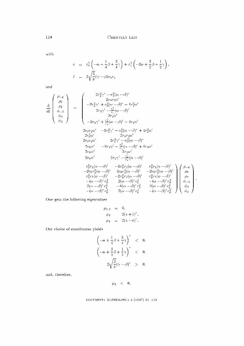
110 Christian Leis

with

s = r

2

0

�

��+

1

4

� +

3

4

�

+ r

2

2

�

�2�+

3

2

� +

1

2

�

;

t = 2

r

3

8

( � �)r

0

r

2

and

d

dt

0

B

B

B

B

B

B

@

�

�2

�

0

�

2

�

�2

�

0

�

2

1

C

C

C

C

C

C

A

=

0

B

B

B

B

B

B

B

@

2r

2

2

r

� r

2

0

(� � �)

r

2r

0

r

2

�

r

�2r

2

2

r

+ r

2

0

(�� )

r

+ 4r

2

2

�

r

2r

2

i

�

r

2

0

r

2

(�� )

i

2r

2

�

i

�2r

2

i

+

r

2

0

r

2

(�� )

i

+ 4r

2

�

i

2r

0

r

2

�

r

�2r

2

2

r

+ r

2

0

(�� )

r

+ 4r

2

2

�

r

2r

2

0

�

r

2r

0

r

2

�

r

2r

0

r

2

�

r

2r

2

2

r

� r

2

0

(�� )

r

2r

0

�

i

�2r

2

i

+

r

2

0

r

2

(�� )

i

+ 4r

2

�

i

2r

0

�

i

2r

2

�

i

2r

0

�

i

2r

2

i

�

r

2

0

r

2

(�� )

i

r

2

0

r

2

(�� )

i

�2r

2

0

r

2

(�� )

i

r

2

0

r

2

(�� )

i

�2r

0

r

2

2

(�� )

i

4r

0

r

2

2

(�� )

i

�2r

0

r

2

2

(�� )

i

r

2

0

r

2

(�� )

i

�2r

2

0

r

2

(�� )

i

r

2

0

r

2

(�� )

i

�(�� )

r

r

2

0

2(�� )

r

r

2

0

�(�� )

r

r

2

0

2(�� )

r

r

2

2

�4(�� )

r

r

2

2

2(�� )

r

r

2

2

�(�� )

r

r

2

0

2(�� )

r

r

2

0

�(�� )

r

r

2

0

1

C

C

C

C

C

C

A

0

B

B

B

B

B

B

@

�

�2

�

0

�

2

�

�2

�

0

�

2

1

C

C

C

C

C

C

A

:

One gets the following eigenvalues

�

1;2

= 0;

�

3

= 2(s + t)

r

;

�

4

= 2(s � t)

r

:

Our choice of coordinates yields

�

��+

1

4

� +

3

4

�

r

< 0;

�

��+

3

4

� +

1

4

�

r

< 0;

2

r

3

8

( � �)

r

> 0;

and, therefore,

�

4

< 0:


Invariant Tori 111

Finally we want to show

�

3

< 0:

By insertion on gets

�

3

= 2

( � �)

r

1

2

r

2

0

+ 2

r

3

8

r

0

r

�

�

2�

r

�

r

2

0

2

!

�

�

2�

r

�

�2�+

3

2

� +

1

2

�

r

!

:

The ansatz

r

2

0

= �t

�

�

r

; t 2

�

0;

1

4

�

;

yields

�

3

= �2

�

�

r

( � �)

r

1

2

t+ 2

r

3

8

r

t(1� t)

2

!

+

1

2

�

�2�+

3

2

� +

1

2

�

r

!

:

In the admissible region we have

�

3

< 0:

The eigenvalues of the second system are (cf. Lemmata 3.5.2 and 3.5.3),

�

1;2;3

= 0;

�

4

= �2� < 0;

�

5

= 2

�

�

r

(� � �)

r

< 0;

�

6

= �2

�

r

2

0

(�� )

r

+ 2r

2

2

(�� )

r

�

:

Therefore in the bifurcation point

~�

1

= �

�(�� )

r

�

r

(� � )

r

there are six trivial and four negative Floquet-exponents. In the entire system the

solution has isotropy (D

2

; 1) in the bifurcation point. Thus the group orbit is four

dimensional. Therefore four trivial exponents are symmetry given. The sign of the

Floquet-exponents of the periodic solution corresponds to the sign of the eigenvalues of

the associated �xed point in the strati�ed space. Dealing with �xed point bifurcation

in the strati�ed space the group orbit of the bifurcating solution inherits the stability

of the bifurcation point. The double zero eigenvalue at the bifurcation point splits

into one positive and one negative eigenvalue (cf. Proposition 3.8.1). Therefore the

bifurcating �xed point is hyperbolic. In the entire system the bifurcating �xed point

has isotropy (Z

2

; 1).

The following lemma is shown.

Lemma 3.9.1 The bifurcating group orbit (cf. Proposition 3.8.1) has the unstable

dimension one.


112 Christian Leis

References

[Bi] Bierstone E., Lifting isotopies from orbit spaces, Topology 14 (1975),

245�252.

[BrtD] Bröcker Th. and T. tom Dieck, Representations of Compact Lie Groups,

GTM, Springer, 1985.

[ChLaMe] Chossat P., R. Lauterbach and I. Melbourne, Steady-State Bifurcation

with O(3)-Symmetry, Arch. Rat. Mech. Anal. 113 (1990), 313�376.

[Co] Conley Ch., Isolated Invariant Sets and the Morse Index, Conf. Board

Math. Sci. 38, AMS, 1978.

[Di] Dieudonné J., Grundzüge der modernen Analysis 3, Vieweg, 1975.

[EletAl] Elphick C., E. Tirapegui, M.E. Brachet, P. Coullet and G. Iooss, A simple

global characterisation for normal forms of singular vector �elds, Physica

D 29 (1987), 95�127.

[Fe] Fenichel N., Geometric Singular Pertubation Theory for Ordinary Di�er-

ential Equations, J. Di�. Eqns. 31 (1979), 53�89.

[Fi] Fiedler B., Global Bifurcations of Periodic Solutions with Symmetry, Lec-

ture Notes in Math. 1309, Springer, 1988.

[FiMi] Fiedler B. and K. Mischaikow, Dynamics of Bifurcations for Variational

Problems with O(3) Equivariance: A Conley Index Approach, Arch. Rat.

Mech. Anal. 119 (1992), 145�196.

[HaRoSt] Haaf H., M. Roberts and I. Stewart, A Hopf bifurcation with symmetry,

ZAMP 43 (1992), 793�826.

[IoRo] Iooss G. and M. Rossi, Hopf bifurcation in the presence of spherical sym-

metry: Analytical Results, SIAM J. Math. Anal. 20 No 3 (1989), 511�532.

[GoSt] Golubitsky M. and I. Stewart, Hopf Bifurcation in the Presence of Sym-

metry, Arch. Rat. Mech. Anal. 87 No 2 (1985), 107�165.

[GoStSch] Golubitsky M., I. Stewart and D. Schae�er, Singularities and Groups in

Bifurcation Theory II, Appl. Math. Sci. 69, Springer, 1988.

[La1] Lauterbach R., Bifurcation with O(3)-symmetry, Habilitationsschrift, Uni-

versität Augsburg, 1988.

[La2] Lauterbach R., Äquivariante Dynamische Systeme, Skript, FU-Berlin,

1995.

[Le] Leis Ch., Hopf-Bifurcation in Systems with Spherical Symmetry Part II :

Connecting Orbits, to appear in J. reine angew. Math.

[Mi] Miller W., Symmetry groups and their application, Acad. Press., 1972.


Invariant Tori 113

[MoRoSt] Montaldi J., M. Roberts and I. Stewart, Stability of nonlinear normal

modes of symmetric Hamiltonian systems, Nonlinearity 3 (1990), 731�

722.

[Sa] Sattinger D.H., Group Theoretic Methods in Bifurcation Theory, Lecture

Notes in Math. 762, Springer, 1979.

[StiFä] Stiefel E. and A. Fässler, Gruppentheoretische Methoden und ihre An-

wendung, Teubner, 1979.

Christian Leis

FU-Berlin

Institut für Mathematik

Arnimallee 2-6

14195 Berlin, Germany

E-Mail: leismath.fu-berlin.de


114

Documenta Mathematica 2 (1997)

62 - univie.ac.at · () fix t arian v in as a subspace. w no e w shall lo ok at the tation represen...

Documents