689 ' # '5& *#6 & 7cdn.intechopen.com/pdfs-wm/33344.pdf · the atmosphere of the...

3,350+OPEN ACCESS BOOKS

108,000+INTERNATIONAL

AUTHORS AND EDITORS115+ MILLION

DOWNLOADS

BOOKSDELIVERED TO

151 COUNTRIES

AUTHORS AMONG

TOP 1%MOST CITED SCIENTIST

12.2%AUTHORS AND EDITORS

FROM TOP 500 UNIVERSITIES

Selection of our books indexed in theBook Citation Index in Web of Science™

Core Collection (BKCI)

Chapter from the book Solar RadiationDownloaded from: http://www.intechopen.com/books/solar-radiation

PUBLISHED BY

World's largest Science,Technology & Medicine

Open Access book publisher

Interested in publishing with IntechOpen?Contact us at [email protected]

http://www.intechopen.com/books/solar-radiation

mailto:[email protected]

1. Introduction

High altitude astronomical sites are a scarce commodity with increasing demand. A thinatmosphere can make a substantial difference in the performance of scientific researchinstruments like millimeter-wave telescopes or water Cerenkov observatories. In our planetreaching above an altitude of 4000 m involves confronting highly adverse meteorologicalconditions. Sierra Negra, the site of the Large Millimeter Telescope (LMT) is exceptional inbeing one of the highest astronomical sites available with endurable weather conditions.

One of the most important considerations to characterize a ground-based astronomicalobservatory is cloud cover. Given a site, statistics of daytime cloud cover indicate the usableportion of the time for optical and near-infrared observations and bring key information forthe potentiality of that site for millimeter and sub-millimeter astronomy. The relationshipbetween diurnal and nocturnal cloudiness is strongly dependent on the location of the site (1).For several astronomical sites it has been reported (1) that the day versus night variation ofthe cloud cover is less than 5 %. Therefore, daytime cloud cover statistics is a useful indicatorof nighttime cloud conditions.

We developed a model for the radiation that allowed us to estimate the fraction of time whenthe sky is clear of clouds. It consists of the computation of histograms of solar radiation valuesmeasured at the site and corrected for the zenithal angle of the Sun.

The model was applied to estimate the daytime clear fraction for Sierra Negra (2). Theresults obtained are consistent with values reported by other authors using satellite data(1). The same method was applied to estimate the cloud cover of San Pedro Mártir -anotherastronomical site (3) . The estimations of the time when the sky is clear of clouds obtainedare also consistent with those reported by the same authors (1). The consistency of our results

A New Method to Estimate the Temporal Fraction of Cloud Cover

Esperanza Carrasco1, Alberto Carramiñana1, Remy Avila2, Leonardo J. Sánchez3 and Irene Cruz-González3

1Instituto Nacional de Astrofísica, Óptica y Electrónica, Puebla

2Centro de Física Aplicada y Tecnología Avanzada Universidad Nacional Autónoma de México,

Santiago de Querétaro 3Instituto de Astronomía,

Universidad Nacional Autónoma de México, México D.F.

México

4

www.intechopen.com

2 Solar radiation

with those obtained applying different and classical techniques shows the great potential ofthe method developed to estimate cloud cover from in situ measurements.

In this chapter our model will be explained. In §2 the main characteristics of solar radiationthrough the terrestrial atmosphere are discussed; in §3 our method to estimate the temporalfraction of cloud cover is described using radiation data of the astronomical sites Sierra Negraand San Pedro Mártir. In §4 a brief summary is presented.

2. Solar radiation through the terrestrial atmosphere

2.1 The Sun

The Sun provides energy to the Earth at an average rate of s⊙ = 1367 W/m2. This valuerelates directly to the solar luminosity, L⊙ = 3.84(4) × 1027Watts, as observed at an averagedistance of one astronomical unit, s⊙ = L⊙/

(

4πd2⊕)

, with d⊕ = 1 UA ≃ 1.496 × 1011 m.The value of s⊙ is stable enough to be often referred as the Solar constant. Variations of thesolar flux arise from intrinsic variations in the solar luminosity and seasonal variations of thedistance between the Earth and the Sun. The eccentricity of the orbit of the Earth around theSun, ε⊕ = 0.0167, translates into minimum and maximum distances of d⊕/(1 ± ε), and hencea yearly modulation (∝ ε2

⊕) of ±3.3% in the solar flux over the year. Given a location on theEarth, this modulation is smaller than seasonal variations due to the changes of the apparenttrajectory of the Sun in the sky, originated by the inclination of the Earth spin axis relative tothe ecliptic. Intrinsic variations of the solar flux due to changes in luminosity, some tentativelyrelated to the 11-year solar activity cycle, are very low, of the order of 0.1%.

The solar radiation is distributed along the infrared to ultraviolet regions of theelectromagnetic spectrum. This distribution is shown in terms of apparent magnitudes mν instandard spectral bands, from the ultraviolet (U) to the infrared (IHJK), in Table 1 and plottedin Fig. 1. The conversion into energy flux Fν is made through the standard formula:

Fν = F0ν 10−0.4mν . (1)

A comparison of the solar spectrum with a blackbody spectrum can be made defining threetemperature measures: the effective temperature; the color temperature; and the brightnesstemperature:

• the effective temperature Te is given by the integrated flux F and the angular size of theradiation source, F = σT4

e δθ2, with δθ the apparent radius and σ the Stefan Boltzmannconstant. For the Sun Te ≃ 5770 K, which corresponds to a maximum emission at awavelength λ ≃ 0.5 µm.

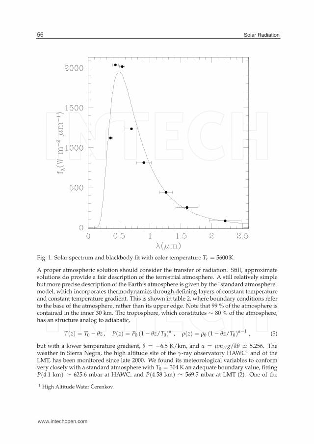
• the color temperature is calculated through the best blackbody fit of the spectrum. Fig. 1shows a blackbody fit to Fν of the form Aν3/(eν/νc − 1), with best fit parameters

A = 1.166 × 10−9erg cm−2s−1, and νc = 1.167 × 1014 Hz , (2)

which result in a color temperature Tcol ≃ 5600 K. As observed in the plot, a blackbody isa fair fit of the spectral distribution of the solar flux.

• the third temperature indicator of solar conditions is the brightness temperature, definedmonocromatically by Iν = Bν(Tb). It is nearest to the effective temperature in the I band,λ = 0.9 µm.

54 Solar Radiation

www.intechopen.com

A New Method to Estimate the Temporal Fraction of Cloud Cover 3

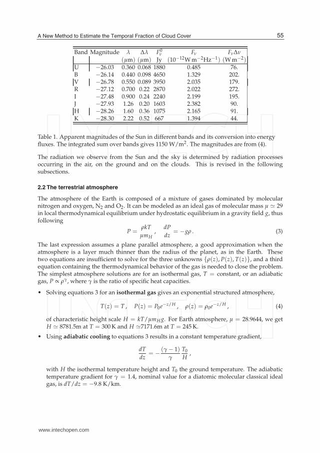
Band Magnitude λ ∆λ F0ν Fν Fν∆ν

(µm) (µm) Jy (10−12W m−2Hz−1) (W m−2)U −26.03 0.360 0.068 1880 0.485 76.B −26.14 0.440 0.098 4650 1.329 202.V −26.78 0.550 0.089 3950 2.035 179.R −27.12 0.700 0.22 2870 2.022 272.I −27.48 0.900 0.24 2240 2.199 195.J −27.93 1.26 0.20 1603 2.382 90.H −28.26 1.60 0.36 1075 2.165 91.K −28.30 2.22 0.52 667 1.394 44.

Table 1. Apparent magnitudes of the Sun in different bands and its conversion into energyfluxes. The integrated sum over bands gives 1150 W/m2. The magnitudes are from (4).

The radiation we observe from the Sun and the sky is determined by radiation processesoccurring in the air, on the ground and on the clouds. This is revised in the followingsubsections.

2.2 The terrestrial atmosphere

The atmosphere of the Earth is composed of a mixture of gases dominated by molecularnitrogen and oxygen, N2 and O2. It can be modeled as an ideal gas of molecular mass µ ≃ 29in local thermodynamical equilibrium under hydrostatic equilibrium in a gravity field g, thusfollowing

P =ρkT

µmH,

dP

dz= −gρ . (3)

The last expression assumes a plane parallel atmosphere, a good approximation when theatmosphere is a layer much thinner than the radius of the planet, as in the Earth. Thesetwo equations are insufficient to solve for the three unknowns {ρ(z), P(z), T(z)}, and a thirdequation containing the thermodynamical behavior of the gas is needed to close the problem.The simplest atmosphere solutions are for an isothermal gas, T = constant, or an adiabaticgas, P ∝ ργ, where γ is the ratio of specific heat capacities.

• Solving equations 3 for an isothermal gas gives an exponential structured atmosphere,

T(z) = T , P(z) = P0e−z/H , ρ(z) = ρ0e−z/H , (4)

of characteristic height scale H = kT/µmH g. For Earth atmosphere, µ = 28.9644, we getH ≃ 8781.5m at T = 300 K and H ≃7171.6m at T = 245 K.

• Using adiabatic cooling to equations 3 results in a constant temperature gradient,

dT

dz= − (γ − 1)

γ

T0

H,

with H the isothermal temperature height and T0 the ground temperature. The adiabatictemperature gradient for γ = 1.4, nominal value for a diatomic molecular classical idealgas, is dT/dz = −9.8 K/km.

55A New Method to Estimate the Temporal Fraction of Cloud Cover

www.intechopen.com

4 Solar radiation

Fig. 1. Solar spectrum and blackbody fit with color temperature Tc = 5600 K.

A proper atmospheric solution should consider the transfer of radiation. Still, approximatesolutions do provide a fair description of the terrestrial atmosphere. A still relatively simplebut more precise description of the Earth’s atmosphere is given by the "standard atmosphere"model, which incorporates thermodynamics through defining layers of constant temperatureand constant temperature gradient. This is shown in table 2, where boundary conditions referto the base of the atmosphere, rather than its upper edge. Note that 99 % of the atmosphere iscontained in the inner 30 km. The troposphere, which constitutes ∼ 80 % of the atmosphere,has an structure analog to adiabatic,

T(z) = T0 − θz , P(z) = P0 (1 − θz/T0)α , ρ(z) = ρ0 (1 − θz/T0)

α−1 , (5)

but with a lower temperature gradient, θ = −6.5 K/km, and α = µmH g/kθ ≃ 5.256. Theweather in Sierra Negra, the high altitude site of the γ-ray observatory HAWC1 and of theLMT, has been monitored since late 2000. We found its meteorological variables to conformvery closely with a standard atmosphere with T0 = 304 K an adequate boundary value, fittingP(4.1 km) ≃ 625.6 mbar at HAWC, and P(4.58 km) ≃ 569.5 mbar at LMT (2). One of the

1 High Altitude Water Cerenkov.

56 Solar Radiation

www.intechopen.com


Capa zg0 z0 dT/dz T0 P0

(km) (km) K/km ◦C PaTroposphere 0 0.000 −6.5 +15.0 101 325Tropopause 11 11.019 0.0 −56.5 22 632Stratosphere (I) 20 20.063 +1.0 −56.5 5 475Stratosphere (II) 32 32.162 +2.8 −44.5 868Stratopause 47 47.350 0.0 −2.5 111Mesosphere (I) 51 51.413 −2.8 −2.5 67Mesosfera (II) 71 71.802 −2.0 −58.5 4Mesopause 84.852 86.000 −− −86.2 0.37

Table 2. Layers defining the International Standard Atmosphere. zg0 y z0 are the geopotentialand geometric heights, respectively, at the base of the layer.

ongoing projects at the Sierra Negra site is the simultaneous measurements of meteorologicalvariables, and hence their gradients, in these two locations.

2.3 The transfer of solar radiation through the atmosphere

One of the most important features of the terrestrial atmosphere is its transparency to visiblelight, while being opaque to infrared radiation. As a consequence, most of the solar radiationreaches the ground, where it is thermalized and re-emitted as infrared radiation, which istrapped by atmospheric molecules, raising Earth’s temperature above its direct equilibriumtemperature. This is the basic scenario of our atmosphere; in practice this is complicatedby scattering due to small particles suspended in the air, the presence of clouds, the localproperties of the ground and the sea, and the non static conditions in the atmosphere (winds)and the sea (currents).

In the absence of an atmosphere, the temperature on a location where the Sun is observedwith an angle θ⊙ would be given by the equilibrium condition

(1 − a)s⊙ cos θ⊙ = πσT4, (6)

where a represent the albedo, or fraction of the radiation reflected by the surface, and the factorπ results from integrating the re-emitted radiation (∝ cos θ) over half a sphere. For an albedo

a = 0.3, the temperature is T ≃ 270 cos θ1/4⊙ K. The radiation emitted by the ground will be

emitted in the infrared, at wavelengths of the order of 10 µm. The resulting simplification isthat radiation in the atmosphere can be treated in terms of two separated components, one inthe visible (λ ≃ 0.5 µm) and the other in the infrared (λ ≃ 10 µm).

A refinement of the previous calculation can be made assuming a grey atmosphere, wherethe term grey indicates the assumption that its radiation properties are independent of thewavelength, at least on a given spectral window. If we now assume the atmosphere absorbs10 % of the visible light and 80 % of the infrared radiation originated on the ground, we inferthat just above 60 % of the solar radiation is trapped by the atmosphere, which acquires atemperature Ta given by the energy density of the radiation captured,

u = aT4a = ηs⊙/c ⇒ T ≃ 245 K, (7)


www.intechopen.com

6 Solar radiation

with η = 0.604 and c the speed of light. As seen in the previous subsection the atmosphere isnot an homogeneous layer, although most of it can be described as in local thermodynamicalequilibrium, with the temperature scale T(z) defined in table 2. The implicit assumptionis that radiation absorption and emission rates are nearly equal locally. Although theyare less abundant than N2 and O2, molecules like water (H2O), carbon dioxide (CO2) andmethane (CH4) play important roles in atmospheric radiation transfer processes. Theirmolecular spectra are rich in electronic, vibrational and rotational transitions. The vibrationalcomponents are important in the infrared while the rotational transitions dominate inmicrowaves.

Relevant to this work are the optical properties of the atmosphere. On the one hand,processes occurring in transparent air and on the other hand, the brightness of clouds.Aerosol particles suspended in the air scatter light, with preferential selection of shorterwavelengths. This process is described in terms of Rayleigh scattering, for which the cross

section can be roughly written as σ ≈ 5.3 × 10−31 m−2 (λ/532 nm)−4. The integration ofthe hydrostatic equilibrium equation (3) shows that the column density of the atmosphereis given by N = P/µmH g ≃ 2.1 × 1029 m3, and a probability N σ ≈ 0.1 of absorbing a532 nm photon in one atmosphere, assuming (wrongly) that the density of aerosol particles isproportional to that of air everywhere in the atmosphere. Taking as a benchmark λ = 0.5 nm,where the solar emission is maximum, the visible emission of the atmosphere downwardsdue to scattering amounts to 5 % of the solar flux distributed over an effective solid angleof π steradians, equivalent to 4.3 mag/arcsec2. This means that even if the direct solarradiation were obstructed, an omnidirectional detector of visible radiation would measurea flux ∼ 0.05s⊙. The fact that Rayleigh scattering is a process whose importance increases atshort wavelengths is well known to be the origin of the blue color of diurnal sky.

The most common situation in which direct solar radiation is obstructed is cloudy weather.In cloudy conditions solar light is scatter and reflected by water particles suspended in theclouds. Without entering in details, one can see that a sizable fraction of solar radiationscattered by the clouds does reach the ground. This amount does depend on the actualconditions, but will add to the 5 % grossly estimated to arise from blue sky itself. The resultsof the studies presented below put the integrated emission of cloudy skies at about 20 % ofs⊙.

3. A method to estimate the temporal fraction of cloud cover

3.1 Introduction

In this section a new method to estimate the temporal fraction of cloud cover, based in solarradiation measurements in situ, will be described. The data are compared with the radiationexpected given the coordinates of the site and hence the position of the Sun in the sky. Itwill be illustrated by using real solar radiation data obtained at two astronomical sites: SierraNegra and San Pedro Mártir (SPM), both in Mexico. First, a brief introduction to the sites andthe data sets will be presented. In the next section the solar modulation is explained. In thefollowing two sections the results obtained for Sierra Negra and the statistics of clear timeare described. In the two subsequent sections an additional example of the method appliedto SPM and the statistics of clear time are discussed. In this case, the model proved to besensitive enough to determine the presence of other atmospheric phenomena.

58 Solar Radiation

www.intechopen.com


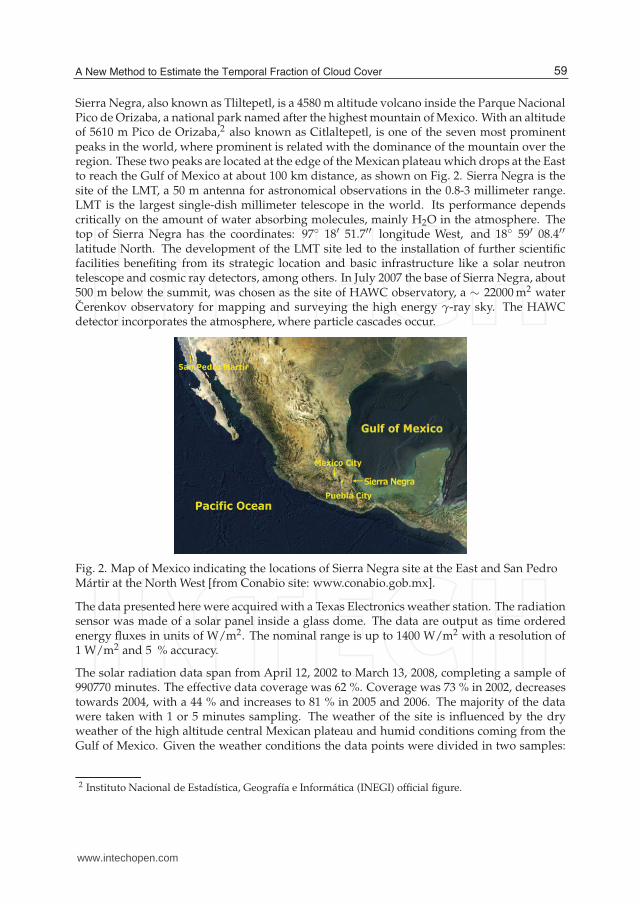
Sierra Negra, also known as Tliltepetl, is a 4580 m altitude volcano inside the Parque NacionalPico de Orizaba, a national park named after the highest mountain of Mexico. With an altitudeof 5610 m Pico de Orizaba,2 also known as Citlaltepetl, is one of the seven most prominentpeaks in the world, where prominent is related with the dominance of the mountain over theregion. These two peaks are located at the edge of the Mexican plateau which drops at the Eastto reach the Gulf of Mexico at about 100 km distance, as shown on Fig. 2. Sierra Negra is thesite of the LMT, a 50 m antenna for astronomical observations in the 0.8-3 millimeter range.LMT is the largest single-dish millimeter telescope in the world. Its performance dependscritically on the amount of water absorbing molecules, mainly H2O in the atmosphere. Thetop of Sierra Negra has the coordinates: 97◦ 18′ 51.7′′ longitude West, and 18◦ 59′ 08.4′′

latitude North. The development of the LMT site led to the installation of further scientificfacilities benefiting from its strategic location and basic infrastructure like a solar neutrontelescope and cosmic ray detectors, among others. In July 2007 the base of Sierra Negra, about500 m below the summit, was chosen as the site of HAWC observatory, a ∼ 22000 m2 waterCerenkov observatory for mapping and surveying the high energy γ-ray sky. The HAWCdetector incorporates the atmosphere, where particle cascades occur.

Fig. 2. Map of Mexico indicating the locations of Sierra Negra site at the East and San PedroMártir at the North West [from Conabio site: www.conabio.gob.mx].

The data presented here were acquired with a Texas Electronics weather station. The radiationsensor was made of a solar panel inside a glass dome. The data are output as time orderedenergy fluxes in units of W/m2. The nominal range is up to 1400 W/m2 with a resolution of1 W/m2 and 5 % accuracy.

The solar radiation data span from April 12, 2002 to March 13, 2008, completing a sample of990770 minutes. The effective data coverage was 62 %. Coverage was 73 % in 2002, decreasestowards 2004, with a 44 % and increases to 81 % in 2005 and 2006. The majority of the datawere taken with 1 or 5 minutes sampling. The weather of the site is influenced by the dryweather of the high altitude central Mexican plateau and humid conditions coming from theGulf of Mexico. Given the weather conditions the data points were divided in two samples:

2 Instituto Nacional de Estadística, Geografía e Informática (INEGI) official figure.


www.intechopen.com

8 Solar radiation

the dry season is the 181 day period from November 1st to April 30; the wet season goes fromMay 1st to October 31st, covering 184 days.

The SPM observatory is located at 31◦02′39′′ latitude North , 115◦27′49′′ longitude West andat an altitude of 2830 m, inside the Parque Nacional Sierra de San Pedro Mártir. SPM is∼65 km E of the Pacific Coast and ∼55 km W to the Gulf of California, as shown in Fig.2. The largest telescope at the site is an optical 2.1-m Ritchey-Chrétien, operational since 1981.Astroclimatological characterization studies at SPM are reviewed in (5). Other aspects of thesite characterization have been reported by several authors e.g. (7; 8). Nevertheless, the firststudy on the radiation data measured in situ was done by Carrasco and collaborators (3). Thedata were recorded by the Thirty Meter Telescope (TMT) site-testing team from 2004 to 2008.See (9) for an overview of the TMT project and its main results.

The data presented here consist of records of solar radiation energy fluxes in units of Wm−2

acquired with an Monitor automatic weather station (9). The sensor has a spectral responsebetween 400 and 950 nm with an accuracy of 5 %, according to the vendor. The data spanfrom 2005 January 12 to 2008 August 8, with a sampling time of 2 minutes and a 67 % effectivecoverage of the 3.6 year sample; data exist for 973 out of 1316 days. The complete samplecontains 596580 min out of 899520 possible; coverage was 59 % for 2005 and increased to 78 %towards the end of the campaign, in 2008.

3.2 Solar modulation

The method to estimate the temporal fraction of cloud coverage is based on computing theratio between the expected amount of radiation and that observed. We safely assume that, atleast under clear conditions, radiation directly received from the Sun is dominant. This is aterm of the form s⊙ cos θ⊙, where θ⊙ is the zenith angle of the Sun as observed from the siteunder study. The modulation term is removed by simply dividing by cos θ⊙. To compute thelocal zenith angle as a function of time, consider a coordinate system centered on Earth withthe z axis oriented perpendicular to the ecliptic. By definition, the position of the Sun in thissystem is restricted to the x − y plane, and is given by d⊕ r⊙, with the direction to the Sungiven by the unitary vector

r⊙ = −x cos (ωat)− y sin (ωat) , (8)

where ωa = 2π/year is the angular frequency associated to the yearly modulation. Given alocation on Earth of geographical latitude b, the zenith is in the direction given by the unitaryvector

n = −ze sin b + (xe cos(ωst) + ye sin(ωst)) cos b, (9)

where ωs = ωa + ωd = 2π/yr + 2π/day, and

xe = x , ye = y cos ı − z sin ı , ze = y sin ı + z cos ı, (10)

with ı the inclination angle of the Earth axis relative to the z, the unitary vector normal to theecliptic plane. With these relations in hand, it follows that the zenith angle of the Sun is givenby cos θ⊙ = −n · r⊙. Equations 8 and 9 assume t = 0 corresponds to the time of equinox,rather than the beginning of the civil year.

These equations were used to generate solar zenith angles for all years covered by the data.Before the actual data analysis, we verified the proper functioning of the related software, both

60 Solar Radiation

www.intechopen.com


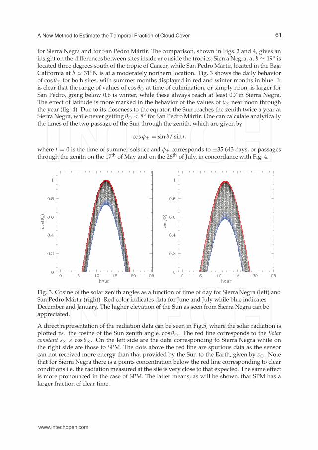
for Sierra Negra and for San Pedro Mártir. The comparison, shown in Figs. 3 and 4, gives aninsight on the differences between sites inside or ouside the tropics: Sierra Negra, at b ≃ 19◦ islocated three degrees south of the tropic of Cancer, while San Pedro Mártir, located in the BajaCalifornia at b ≃ 31◦N is at a moderately northern location. Fig. 3 shows the daily behaviorof cos θ⊙ for both sites, with summer months displayed in red and winter months in blue. Itis clear that the range of values of cos θ⊙ at time of culmination, or simply noon, is larger forSan Pedro, going below 0.6 is winter, while these always reach at least 0.7 in Sierra Negra.The effect of latitude is more marked in the behavior of the values of θ⊙ near noon throughthe year (fig. 4). Due to its closeness to the equator, the Sun reaches the zenith twice a year atSierra Negra, while never getting θ⊙ < 8◦ for San Pedro Mártir. One can calculate analyticallythe times of the two passage of the Sun through the zenith, which are given by

cos φ± = sin b/ sin ı,

where t = 0 is the time of summer solstice and φ± corresponds to ±35.643 days, or passagesthrough the zenitn on the 17th of May and on the 26th of July, in concordance with Fig. 4.

Fig. 3. Cosine of the solar zenith angles as a function of time of day for Sierra Negra (left) andSan Pedro Mártir (right). Red color indicates data for June and July while blue indicatesDecember and January. The higher elevation of the Sun as seen from Sierra Negra can beappreciated.

A direct representation of the radiation data can be seen in Fig.5, where the solar radiation isplotted vs. the cosine of the Sun zenith angle, cos θ⊙. The red line corresponds to the Solarconstant s⊙ × cos θ⊙. On the left side are the data corresponding to Sierra Negra while onthe right side are those to SPM. The dots above the red line are spurious data as the sensorcan not received more energy than that provided by the Sun to the Earth, given by s⊙. Notethat for Sierra Negra there is a points concentration below the red line corresponding to clearconditions i.e. the radiation measured at the site is very close to that expected. The same effectis more pronounced in the case of SPM. The latter means, as will be shown, that SPM has alarger fraction of clear time.


www.intechopen.com

10 Solar radiation

Fig. 4. Minimum zenith angle for the Sun as seen from Sierra Negra (left) and San PedroMártir (right). Data shown are for four 10 minute windows at or close to the local time ofculmination, or solar noon. The Sun reaches the zenith (θ⊙ = 0◦) twice a year in SierraNegra, while ranging from 55◦ to 7◦ at San Pedro.

Fig. 5. Solar power versus cos θ⊙ global and per year. The red line corresponds tos⊙ × cos θ⊙. Left: for Sierra Negra. Right: for San Pedro Mártir

3.3 The histogram of ψ(t) for Sierra Negra

The radiation flux at ground level is considered, to first approximation, to be given by theSolar constant s⊙, modulated by the zenith angle of the Sun and a time variable attenuationfactor ψ(t). Knowing the position of the Sun at the site as a function of time, we can estimate

62 Solar Radiation

www.intechopen.com


the variable ψ, given as

ψ(t) =F(t)

s⊙ cos θ⊙. (11)

where F(t) is the radiation measured at the site and θ⊙ is the zenith angle of the Sun. ψ(t) isa time variable factor, nominally below unity, which accounts for the instrumental response(presumed constant), the atmospheric extinction on site and the effects of the cloud coverage.

Knowing the site latitude, the modulation factor cos θ⊙ was computed as a function of day,month and local time, minute per minute to study the behavior of the variable ψ and to obtainits distribution. The term z is referred as the airmass, defined as z = sec θ⊙; thus z < 2 isequivalent to θ⊙ < 60◦ . Most astronomical observations are carry out at this airmass interval.

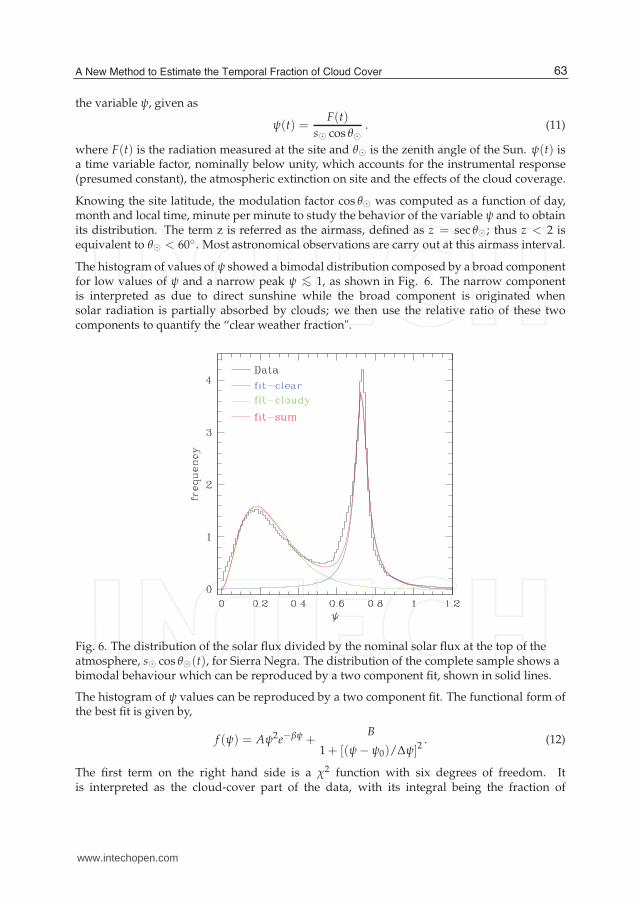
The histogram of values of ψ showed a bimodal distribution composed by a broad componentfor low values of ψ and a narrow peak ψ <∼ 1, as shown in Fig. 6. The narrow componentis interpreted as due to direct sunshine while the broad component is originated whensolar radiation is partially absorbed by clouds; we then use the relative ratio of these twocomponents to quantify the “clear weather fraction".

Fig. 6. The distribution of the solar flux divided by the nominal solar flux at the top of theatmosphere, s⊙ cos θ⊙(t), for Sierra Negra. The distribution of the complete sample shows abimodal behaviour which can be reproduced by a two component fit, shown in solid lines.

The histogram of ψ values can be reproduced by a two component fit. The functional form ofthe best fit is given by,

f (ψ) = Aψ2e−βψ +B

1 + [(ψ − ψ0)/∆ψ]2. (12)

The first term on the right hand side is a χ2 function with six degrees of freedom. Itis interpreted as the cloud-cover part of the data, with its integral being the fraction of


www.intechopen.com

12 Solar radiation

cloud-covered time. The second term, a Lorentzian function with centre ψ0 and width ∆ψ,represents the cloud-clear part of the data. A and B provide the normalization and relativeweights of both components; β is related to the width and centre of the broad peak. Inthe appendix the details of the calculation of the fit parameters, including the errors, arediscussed.

In Fig. 6 the distribution of ψ for the whole data set is shown in black with the doublecomponent fit in red. The first component of the fit corresponding to the cloud cover partof the data is shown in blue while the second one, corresponding to the clear part of the datais shown in green. This bimodal distribution, with a first maximum at around ψ ∼ 0.2 and anarrow peak at ψ ∼ 0.75, has a minimum around ψ ∼ 0.55.

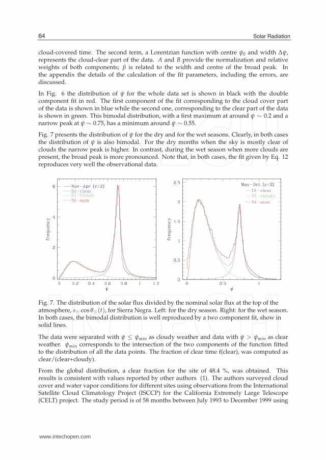
Fig. 7 presents the distribution of ψ for the dry and for the wet seasons. Clearly, in both casesthe distribution of ψ is also bimodal. For the dry months when the sky is mostly clear ofclouds the narrow peak is higher. In contrast, during the wet season when more clouds arepresent, the broad peak is more pronounced. Note that, in both cases, the fit given by Eq. 12reproduces very well the observational data.

Fig. 7. The distribution of the solar flux divided by the nominal solar flux at the top of theatmosphere, s⊙ cos θ⊙(t), for Sierra Negra. Left: for the dry season. Right: for the wet season.In both cases, the bimodal distribution is well reproduced by a two component fit, show insolid lines.

The data were separated with ψ ≤ ψmin as cloudy weather and data with ψ > ψmin as clearweather. ψmin corresponds to the intersection of the two components of the function fittedto the distribution of all the data points. The fraction of clear time f(clear), was computed asclear/(clear+cloudy).

From the global distribution, a clear fraction for the site of 48.4 %, was obtained. Thisresults is consistent with values reported by other authors (1). The authors surveyed cloudcover and water vapor conditions for different sites using observations from the InternationalSatellite Cloud Climatology Project (ISCCP) for the California Extremely Large Telescope(CELT) project. The study period is of 58 months between July 1993 to December 1999 using

64 Solar Radiation

www.intechopen.com


a methodology that had been tested and successfully applied in previous studies. For SierraNegra they measured a clear fraction for nighttime of 47 %. They conclude that the day versusnight variation of cloud cover is less than 5 %, being clearer at night. Therefore, the resultsobtained with the method presented here are consistent within 6.4 % with those obtained viaa totally independent technique.

3.4 Statistics of clear time for Sierra Negra

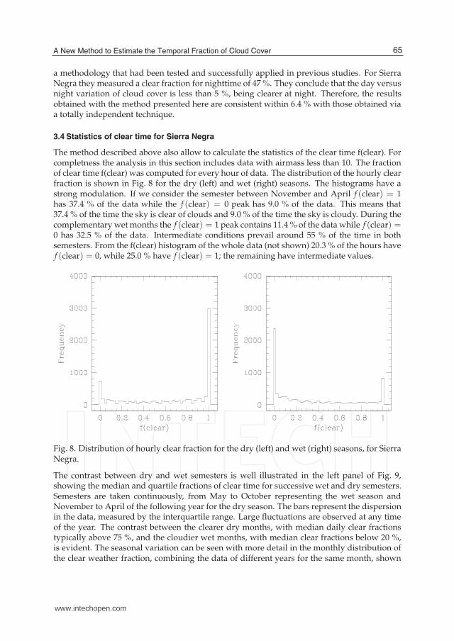
The method described above also allow to calculate the statistics of the clear time f(clear). Forcompletness the analysis in this section includes data with airmass less than 10. The fractionof clear time f(clear) was computed for every hour of data. The distribution of the hourly clearfraction is shown in Fig. 8 for the dry (left) and wet (right) seasons. The histograms have astrong modulation. If we consider the semester between November and April f (clear) = 1has 37.4 % of the data while the f (clear) = 0 peak has 9.0 % of the data. This means that37.4 % of the time the sky is clear of clouds and 9.0 % of the time the sky is cloudy. During thecomplementary wet months the f (clear) = 1 peak contains 11.4 % of the data while f (clear) =0 has 32.5 % of the data. Intermediate conditions prevail around 55 % of the time in bothsemesters. From the f(clear) histogram of the whole data (not shown) 20.3 % of the hours havef (clear) = 0, while 25.0 % have f (clear) = 1; the remaining have intermediate values.

Fig. 8. Distribution of hourly clear fraction for the dry (left) and wet (right) seasons, for SierraNegra.

The contrast between dry and wet semesters is well illustrated in the left panel of Fig. 9,showing the median and quartile fractions of clear time for successive wet and dry semesters.Semesters are taken continuously, from May to October representing the wet season andNovember to April of the following year for the dry season. The bars represent the dispersionin the data, measured by the interquartile range. Large fluctuations are observed at any timeof the year. The contrast between the clearer dry months, with median daily clear fractionstypically above 75 %, and the cloudier wet months, with median clear fractions below 20 %,is evident. The seasonal variation can be seen with more detail in the monthly distribution ofthe clear weather fraction, combining the data of different years for the same month, shown


www.intechopen.com

14 Solar radiation

Fig. 9. Left: clear fractions for the different seasons. Points are at median; bars go from 1st to3rd quartile. Wet season (open dots) is the yearly interval from May to October; dry season(full dots) is from November to April of the following year. Right: the median and quartilevalues of the fraction of clear weather for the different months of the year.

Fig. 10. Left: median and quartile values of the fraction of clear weather fclear, for each hourof day. The lower and upper panels are for wet (MJJASO) and dry (NDJFMA) semesters,respectively. Right: a grey level plot showing the median fraction of clear time f(clear), foreach month and hour of day. Squares are drawn when more than 10 h of data are available;crosses indicate less than 10 h of data.

on the right side of the same figure. The skies are clear, f(clear)> 80 %, between Decemberand March, fair in April and November, f(clear)∼ 60 %, and poor between May and October,

66 Solar Radiation

www.intechopen.com


f(clear)< 30 %. The fluctuations in the data are such that clear fractions above 55 % can befound 25 % of the time, even in the worst observing months.

Fig. 10 (left) shows the median and quartile clear fractions as function of hour of day for thewet/dry subsets. The interquartile range practically covers the (0-1) interval at most times.We note that good conditions are more common in the mornings of the dry semesters, whilethe worst conditions prevail in the afternoon of the wet season, dominated by Monsoon rainstorms. The trend in our results for daytime is consistent with that obtained by applyingdifferent methods (1). By analysing the clear fraction during day and nighttime these authorsfound that the clear fraction is highest before noon, has a minimum in the afternoon andincreases during nighttime.

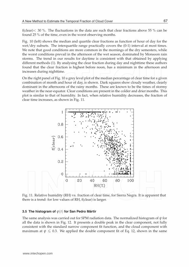
On the right panel of Fig. 10 a grey level plot of the median percentage of clear time for a givencombination of month and hour of day, is shown. Dark squares show cloudy weather, clearlydominant in the afternoons of the rainy months. These are known to be the times of stormyweather in the near-equator. Clear conditions are present in the colder and drier months. Thisplot is similar to that of humidity. In fact, when relative humidity decreases, the fraction ofclear time increases, as shown in Fig. 11.

Fig. 11. Relative humidity (RH) vs. fraction of clear time, for Sierra Negra. It is apparent thatthere is a trend: for low values of RH, f(clear) is larger.

3.5 The histogram of ψ(t) for San Pedro Mártir

The same analysis was carried out for SPM radiation data. The normalized histogram of ψ forall the data is shown in Fig. 12. It presents a double peak in the clear component, not fullyconsistent with the standard narrow component fit function, and the cloud component withmaximum at ψ <∼ 0.3. We applied the double component fit of Eq. 12, shown in the same


www.intechopen.com

16 Solar radiation

figure. The fit for the clear component is drawn in blue, for the cloud component in green andfor the sum in red. The coefficients of the fit and associated errors are presented in Table 3.Fit errors were obtained through a bootstrap analysis using 10000 samples. The fit agreeswith the data within the statistics, except in the wings of the clear peak. Still, the Lorentzianfunction proved to fit much better the data than a Gaussian. The fit can be better appreciatedin a logarithm version shown on the right side of the same figure.

Fig. 12. Left: the normalized observed distribution of ψ for all the data and the correspondingfits for SPM. The blue line is the fit to clear weather; the green one to cloudy weather and thered line to the sum. Right : the logarithm of the normalized observed distribution of ψ and ofthe corresponding fits.

Parameter Global Bootstrap errors relative

z < 2 error (10−3)A 40.8 40.766 ±0.612 15.0β 7.19 7.175 ±0.044 6.2B 6.03 6.035 ±0.055 9.1ψ0 0.815 0.8151 ±0.0002 0.3∆ψ 0.063 0.0629 ±0.0005 7.5f(clear) 0.824 0.8238 ±0.0009 1.1f(cloud) 0.176 0.1762 ±0.0009 5.0

Table 3. Parameters of the fit shown in red Fig. 12.

We considered data with ψ ≤ ψmin, where ψmin = 0.58, as cloudy weather and data withψ > ψmin as clear weather. The value ψmin = 0.58 corresponds to the intersection of thetwo components of the function fitted to the distribution of all data points. As mentioned,the fraction of clear time f(clear), was computed as clear/(clear+cloudy). From the globalhistogram we obtained for SPM a clear fraction for the site of 82.4 %. The errors in thedetermination of f(clear) and f(cloud), were also obtained by generating 10000 bootstrapsamples; they are shown in Table 3.

68 Solar Radiation

www.intechopen.com


The 82.4 % of clear fraction obtained from the global distribution shown in Fig. 12 is similarto that reported using satellite data (1). These authors estimated that the usable fractions ofnightime at SPM was 81 %. Their definition of usable time includes conditions with highcirrus. For the case of SPM, they conclude that the day versus night variation of cloud coveris less than 5 %, being clearer at night. Therefore, the results presented here are consistentwithin 6.4 % with those reported in the literature (1).

Another estimation of the useful observing time at SPM by Tapia (10) reports a 20 yr statisticsof the fractional number of nights with totally clear, partially clear and mostly cloudy based inthe observing log file of the 2.1m telescope night assistants. The author reports a total fractionof useful observing time of 80.8 % and compares his results with those from other authors (1);he concludes that the monthly results from both studies agree within 5 % while for the yearlyfraction, the discrepancies are lower than 2.5 %. Therefore, our results in this case, are alsoconsistent with those obtained with completely different techniques.

Futhermore, when analyzing the fits per month we realized that the Lorentzian fits for theclear weather peak were better than that of the complete dataset: to study the seasonalvariation of ψ we created histograms and the corresponding fits per month. Consider thehistogram and corresponding fit for July and November shown Fig. 13. It can be appreciatedthat the fits reproduce the distribution of ψ very well. The narrow clear component isconsistent with prevailing clear sky conditions, for which the solar radiation reaches the sitewith only the attenuation of the atmosphere. The coefficients of the fits presented in Fig. 13,according to the functional form of f (ψ), Eq. 12, are shown in Table 4. The fits can be bettervalued in the logarithm displays of Fig. 13, presented in Fig. 14. The fits to the complete data(red line), to clear weather (blue line) and to cloudy weather (green line) are indicated.

Fig. 13. The observed distribution of ψ and the two component fit for July (left) andNovember (right). Comparing both plots a shift in the centre of the narrow component isclearly appreciated.

We studied the position of the centre of the peak corresponding to the clear fraction as afunction of the month of each observed year. We found that for every year there is a cyclic


www.intechopen.com

18 Solar radiation

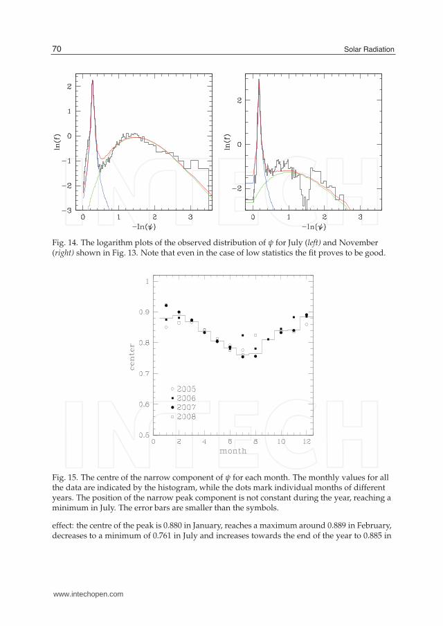
Fig. 14. The logarithm plots of the observed distribution of ψ for July (left) and November(right) shown in Fig. 13. Note that even in the case of low statistics the fit proves to be good.

Fig. 15. The centre of the narrow component of ψ for each month. The monthly values for allthe data are indicated by the histogram, while the dots mark individual months of differentyears. The position of the narrow peak component is not constant during the year, reaching aminimum in July. The error bars are smaller than the symbols.

effect: the centre of the peak is 0.880 in January, reaches a maximum around 0.889 in February,decreases to a minimum of 0.761 in July and increases towards the end of the year to 0.885 in

70 Solar Radiation

www.intechopen.com


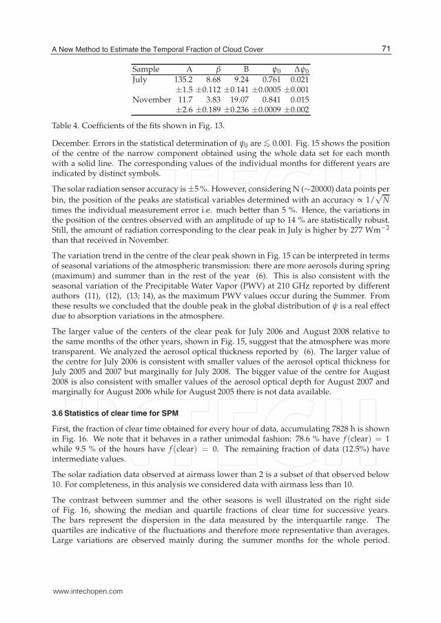
Sample A β B ψ0 ∆ψ0

July 135.2 8.68 9.24 0.761 0.021±1.5 ±0.112 ±0.141 ±0.0005 ±0.001

November 11.7 3.83 19.07 0.841 0.015±2.6 ±0.189 ±0.236 ±0.0009 ±0.002

Table 4. Coefficients of the fits shown in Fig. 13.

December. Errors in the statistical determination of ψ0 are <∼ 0.001. Fig. 15 shows the positionof the centre of the narrow component obtained using the whole data set for each monthwith a solid line. The corresponding values of the individual months for different years areindicated by distinct symbols.

The solar radiation sensor accuracy is ±5 %. However, considering N (∼20000) data points per

bin, the position of the peaks are statistical variables determined with an accuracy ∝ 1/√

Ntimes the individual measurement error i.e. much better than 5 %. Hence, the variations inthe position of the centres observed with an amplitude of up to 14 % are statistically robust.Still, the amount of radiation corresponding to the clear peak in July is higher by 277 Wm−2

than that received in November.

The variation trend in the centre of the clear peak shown in Fig. 15 can be interpreted in termsof seasonal variations of the atmospheric transmission: there are more aerosols during spring(maximum) and summer than in the rest of the year (6). This is also consistent with theseasonal variation of the Precipitable Water Vapor (PWV) at 210 GHz reported by differentauthors (11), (12), (13; 14), as the maximum PWV values occur during the Summer. Fromthese results we concluded that the double peak in the global distribution of ψ is a real effectdue to absorption variations in the atmosphere.

The larger value of the centers of the clear peak for July 2006 and August 2008 relative tothe same months of the other years, shown in Fig. 15, suggest that the atmosphere was moretransparent. We analyzed the aerosol optical thickness reported by (6). The larger value ofthe centre for July 2006 is consistent with smaller values of the aerosol optical thickness forJuly 2005 and 2007 but marginally for July 2008. The bigger value of the centre for August2008 is also consistent with smaller values of the aerosol optical depth for August 2007 andmarginally for August 2006 while for August 2005 there is not data available.

3.6 Statistics of clear time for SPM

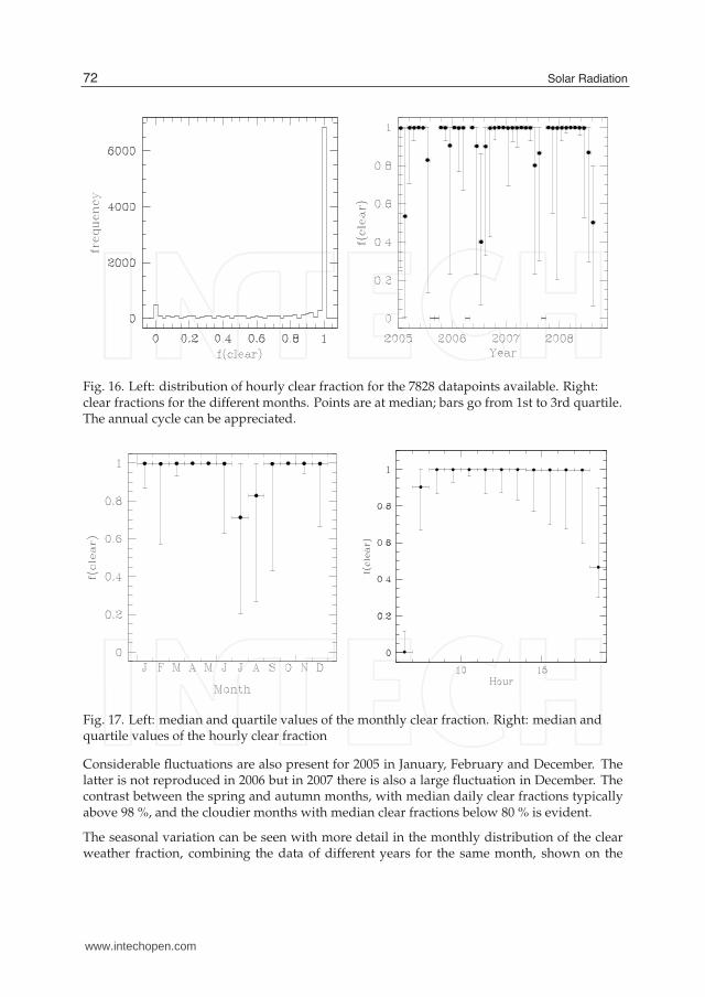
First, the fraction of clear time obtained for every hour of data, accumulating 7828 h is shownin Fig. 16. We note that it behaves in a rather unimodal fashion: 78.6 % have f (clear) = 1while 9.5 % of the hours have f (clear) = 0. The remaining fraction of data (12.5%) haveintermediate values.

The solar radiation data observed at airmass lower than 2 is a subset of that observed below10. For completeness, in this analysis we considered data with airmass less than 10.

The contrast between summer and the other seasons is well illustrated on the right sideof Fig. 16, showing the median and quartile fractions of clear time for successive years.The bars represent the dispersion in the data measured by the interquartile range. Thequartiles are indicative of the fluctuations and therefore more representative than averages.Large variations are observed mainly during the summer months for the whole period.


www.intechopen.com

20 Solar radiation

Fig. 16. Left: distribution of hourly clear fraction for the 7828 datapoints available. Right:clear fractions for the different months. Points are at median; bars go from 1st to 3rd quartile.The annual cycle can be appreciated.

Fig. 17. Left: median and quartile values of the monthly clear fraction. Right: median andquartile values of the hourly clear fraction

Considerable fluctuations are also present for 2005 in January, February and December. Thelatter is not reproduced in 2006 but in 2007 there is also a large fluctuation in December. Thecontrast between the spring and autumn months, with median daily clear fractions typicallyabove 98 %, and the cloudier months with median clear fractions below 80 % is evident.

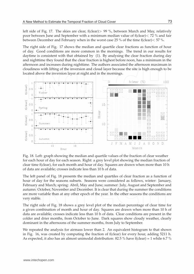
The seasonal variation can be seen with more detail in the monthly distribution of the clearweather fraction, combining the data of different years for the same month, shown on the

72 Solar Radiation

www.intechopen.com


left side of Fig. 17. The skies are clear, f(clear)> 99 %, between March and May, relativelypoor between June and September with a minimum median value of f(clear)< 72 % and fairbetween December and February when in the worst case 25 % of the time f(clear)< 57 %.

The right side of Fig. 17 shows the median and quartile clear fractions as function of hourof day. Good conditions are more common in the mornings. The trend in our results fordaytime is consistent with that obtained by (1). By analysing the clear fraction during dayand nighttime they found that the clear fraction is highest before noon, has a minimum in theafternoon and increases during nighttime. The authors associated the afternoon maximum incloudiness with lifting of the inversion and cloud layer because the site is high enough to belocated above the inversion layer at night and in the mornings.

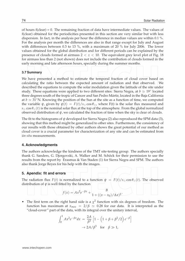
Fig. 18. Left: graph showing the median and quartile values of the fraction of clear weatherfor each hour of day for each season. Right: a grey level plot showing the median fraction ofclear time f(clear), for each month and hour of day. Squares are drawn when more than 10 hof data are available; crosses indicate less than 10 h of data.

The left panel of Fig. 18 presents the median and quartiles of clear fraction as a function ofhour of day for the seasons subsets. Seasons were considered as follows, winter: January,February and March; spring: Abril, May and June; summer: July, August and September andautumn: October, November and December. It is clear that during the summer the conditionsare more variable than at any other epoch of the year. In the other seasons the conditions arevery stable.

The right side of Fig. 18 shows a grey level plot of the median percentage of clear time fora given combination of month and hour of day. Squares are drawn when more than 10 h ofdata are available; crosses indicate less than 10 h of data. Clear conditions are present in thecolder and drier months, from October to June. Dark squares show cloudy weather, clearlydominant in the afternoons of the summer months, from July to September.

We repeated the analysis for airmass lower than 2. An equivalent histogram to that shownin Fig. 16, was created by computing the fraction of f(clear) for every hour, adding 5211 h.As expected, it also has an almost unimodal distribution: 82.5 % have f(clear) = 1 while 6.7 %


www.intechopen.com

22 Solar radiation

of hours f(clear) = 0. The remaining fraction of data have intermediate values. The values off(clear) obtained for the periodicities presented in this section are very similar but with lessdispersion. In fact, in the analysis per hour the difference in median values are within 0.1 %.For the analysis per month the differences are also in that range except for July and Augustwith differences between 0.3 to 13 %, with a maximum of 20 % for July 2006. The lowervalues obtained for the global distribution and for different periods can be explained by thepresence of clouds formed at airmass 2 < z < 10. The equivalent grey level plot of Fig. 18for airmass less than 2 (not shown) does not include the contribution of clouds formed in theearly morning and late afternoon hours, specially during the summer months.

3.7 Summary

We have presented a method to estimate the temporal fraction of cloud cover based oncalculating the ratio between the expected amount of radiation and that observed. Wedescribed the equations to compute the solar modulation given the latitude of the site understudy. These equations were applied to two different sites: Sierra Negra, at b ≃ 19◦ locatedthree degrees south of the tropic of Cancer and San Pedro Mártir, located in the Baja Californiaat b ≃ 31◦N. Knowing the position of the Sun at the site as a function of time, we computedthe variable ψ, given by ψ(t) = F(t)/s⊙ cos θ⊙, where F(t) is the solar flux measured ands⊙ cos θ⊙(t) is the nominal solar flux at the top of the atmosphere. From the global normalizedobserved distribution of ψ, we calculated the fraction of time when the sky is clear of clouds.

The fit to the histograms of ψ developed for Sierra Negra (2) also reproduced the SPM data (3),showing that this method might be generalized to other sites. Furthermore, the consistency ofour results with those obtained by other authors shows the great potential of our method ascloud cover is a crucial parameter for characterization of any site and can be estimated fromiin situ measurements.

4. Acknowledgments

The authors acknowledge the kindness of the TMT site-testing group. The authors speciallythank G. Sanders, G. Djorgovski, A. Walker and M. Schöck for their permission to use theresults from the report by Erasmus & Van Staden (1) for Sierra Negra and SPM. The authorsalso thank Jorge Reyes for his help with the images.

5. Apendix: fit and errors

The radiation flux F(t) is normalized to a function ψ = F(t)/s⊙ cos θ⊙(t). The observeddistribution of ψ is well fitted by the function

f (x) = Ax2e−βx +B

1 + ((x − x0)/∆x)2.

• The first term on the right hand side is a χ2 function with six degrees of freedom. Thefunction has maximum at xmax = 2/β ≃ 0.28 for our data. It is interpreted as the“cloud-cover” part of the data, with its integral over the unitary interval,

∫ 1

0Ax2e−βxdx =

2A

β3

[

1 −(

1 + β + β2/2)

e−β]

→ 2A/β3 for β ≫ 1,

74 Solar Radiation

www.intechopen.com


the fraction of “cloud-covered” time. For the SPM(z < 2) sample we have A = 40.8, β =

7.19 and 2A/β3[

1 −(

1 + β + β2/2)

e−β]

= 0.2195(0.974) = 0.2139. The correct unitary

normalization is for

A∗ =β3/2

1 − (1 + β + β2/2)e−β= 189.74.

• The second term, a Lorentzian function of center x0 and width ∆x, represents the“cloud-clear” part of the data. The fitting function is normalized around x0 such that

∫ x0+η1∆x

x0−η0∆x

B dx

1 + (x − x0/∆x)2= B∆x (arctan(η1) + arctan(η0))

→ Bπ∆x for η0,1 ≫ 1,

the term B∆x(arctan(η1) + arctan(η0)) represents the “clear” fraction. For the SPM(z < 2)data B = 6.03, x0 = 0.8151, ∆x = 0.063, I take η0 = x0/∆x = 12.938 and η1 = (1 −x0)/∆x = 2.935 so arctan η1 + arctan η0 = 0.8709π and the correct normalization factorshould be B∗ = 5.801.

The fit requires determining the five parameters through residual minimization. Thedetermination of {β, x0, ∆x}, determining the shape of the distribution, is numerical; that ofA, B is analytical through solving

⟨

yx2e−βx⟩

= A

⟨

(

x2e−βx)2

⟩

+ B

⟨

x2e−βx

1 + ((x − x0)/∆x)2

⟩

⟨

y

1 + ((x − x0)/∆x)2

⟩

= A

⟨

x2e−βx

1 + ((x − x0)/∆x)2

⟩

+ B

⟨

(

1

1 + ((x − x0)/∆x)2

)2⟩

Strictly speaking, we should have A = (1 − w)A∗ and B = wB∗ with w defining the "clearfraction".

Error determination can, in principle, be done with the process of residual minimization,through a parabolic fit to the function describing the figure of merit. Given the nature ofthe fitting functions this is not practical; we proceeded through a bootstrap analysis of the(z < 2) sample containing N ≃ 180, 000 points, obtaining the results shown in tables 3 and 4.To determine the errors in subsamples of size Ns we assume errors scale as

√N/Ns.

6. References

[1] Erasmus A, & Van Staden C. A., 2002, “A satellite survey of cloud cover and water vaporin the western USA and Northen Mexico. A study conducted for the CELT project.”,internal report

[2] Carrasco, E., Carramiñana, A., Avila, A., Guitérrez, C., Avilés, J.L., Reyes, J., Meza, J. &Yam, O., ( 2009), MNRAS, 398, 407

[3] Carrasco, E., Carramiñana, A., Sánchez, L. J., Avila, R. & Cruz-González, I., (2012),MNRAS, 420, 1273-1280

[4] http://mips.as.arizona.edu/∼cnaw/sun.html[5] Tapia M., Hiriart D., Richer M. & Cruz-González, I.,(2007), Rev. Mex. AA (SC), 31, 47[6] Araiza M.R. & Cruz-González I., (2011) Rev. Mex. AA 47, 409


www.intechopen.com

24 Solar radiation

[7] Cruz-González I., Avila R. & Tapia M., eds, (2003), Rev. Mex. AA (SC), 19.[8] Cruz-González I., Echevarría J. & Hiriart D., eds, (2007), Rev. Mex. AA (SC), 31[9] Schöck M. et al., (2009), Publ. Astr. Soc. Pac., 121, 384

[10] Tapia M., (2003), Rev. Mex. AA (SC), 19, 75[11] Hiriart D. et al., (1997), Rev. Mex. AA, 33, 59[12] Hiriart D. et al., (2003), Rev. Mex. AA (SC), 19, 90[13] Otárola A. et al., (2009), Rev. Mex. AA, 45, 161[14] Otárola A. et al., (2010), Publ. Astr. Soc. Pac., 122, 470

76 Solar Radiation

www.intechopen.com

Solar RadiationEdited by Prof. Elisha B. Babatunde

ISBN 978-953-51-0384-4Hard cover, 484 pagesPublisher InTechPublished online 21, March, 2012Published in print edition March, 2012

InTech EuropeUniversity Campus STeP Ri Slavka Krautzeka 83/A 51000 Rijeka, Croatia Phone: +385 (51) 770 447 Fax: +385 (51) 686 166www.intechopen.com

InTech ChinaUnit 405, Office Block, Hotel Equatorial Shanghai No.65, Yan An Road (West), Shanghai, 200040, China

Phone: +86-21-62489820 Fax: +86-21-62489821

The book contains fundamentals of solar radiation, its ecological impacts, applications, especially inagriculture, architecture, thermal and electric energy. Chapters are written by numerous experienced scientistsin the field from various parts of the world. Apart from chapter one which is the introductory chapter of thebook, that gives a general topic insight of the book, there are 24 more chapters that cover various fields ofsolar radiation. These fields include: Measurements and Analysis of Solar Radiation, Agricultural Application /Bio-effect, Architectural Application, Electricity Generation Application and Thermal Energy Application. Thisbook aims to provide a clear scientific insight on Solar Radiation to scientist and students.

How to referenceIn order to correctly reference this scholarly work, feel free to copy and paste the following:

Esperanza Carrasco, Alberto Carramiñana, Remy Avila, Leonardo J. Sánchez and Irene Cruz-González(2012). A New Method to Estimate the Temporal Fraction of Cloud Cover, Solar Radiation, Prof. Elisha B.Babatunde (Ed.), ISBN: 978-953-51-0384-4, InTech, Available from: http://www.intechopen.com/books/solar-radiation/a-new-method-to-estimate-the-temporal-fraction-of-cloud-cover

689 ' # '5& *#6 & 7cdn.intechopen.com/pdfs-wm/33344.pdf · the atmosphere of the...

Documents