6D Frictional Contact for Rigid BodiesC. Bouchard

McGill University, CanadaM. Nesme

LJK Inria, FranceM. Tournier

RIKEN BSI, BTCC, JapanB. Wang

Shenzhen VisuCA Key Lab, SIAT, China

F. FaureLJK Inria, UJF, France

P. G. Kry∗

McGill University, Canada

ABSTRACT

We present a new approach to modeling contact between rigid ob-jects that augments an individual Coulomb friction point-contactmodel with rolling and spinning friction constraints. Starting fromthe intersection volume, we compute a contact normal from the vol-ume gradient. We compute a contact position from the first momentof the intersection volume, and approximate the extent of the con-tact patch from the second moment of the intersection volume. Byincorporating knowledge of the contact patch into a point contactCoulomb friction formulation, we produce a 6D constraint that pro-vides appropriate limits on torques to accommodate displacementof the center of pressure within the contact patch, while also pro-viding a rotational torque due to dry friction to resist spinning. Acollection of examples demonstrate the power and benefits of thissimple formulation.

Index Terms: Computer Graphics [I.3.5]: Computational Geom-etry and Object Modeling—Physically based modeling

1 INTRODUCTION

Most contact models assume that the contact geometry is a point.While this is sufficient to compute repulsion and friction forces,it does not include enough information to produce resistance torolling or spinning. The rotational behavior of contact only emergesfrom the simultaneous computation of contact forces at multiplepoints.

For an ideal point contact between tangent surfaces, force com-putation typically uses a normal in the direction of the penetrationdepth. When contact surfaces are modeled using multiple contactpoints between pairs of geometric primitives, such as points, trian-gles, and edges, the number of point contacts between two objectscan be large. This results in costly solves, possibly involving sin-gular systems of equations. Additionally, due to the discretizationof time and geometry, the set of contact points can dramaticallychange from one moment to the next. This is especially true whensimulating contact between rigid objects.

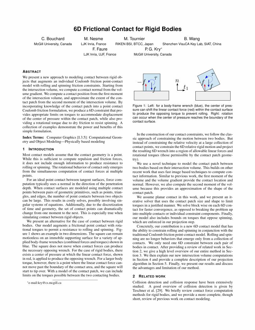
We present an alternative for the case of contact between rigidbodies. Our model augments a frictional point contact with rota-tional torques to permit a resistance to rolling and spinning. Fig-ure 1 shows an example in two dimensions. The square can remainmotionless on an immobile supporting surface for a variety of ap-plied body-frame wrenches (combined forces and torques) shown inblue. The square does not move when contact forces can producethe necessary opposing wrench. For the case of rigid bodies, thereexists a center of pressure at which the linear contact force, shownin red, is applied to produce the opposing wrench. For a larger bodytorque, however, there is a point where the linear contact force can-not move past the boundary of the contact area, and the square willstart to tip over. With a model of the contact patch, we can includelimits on the torques possible between the two contacting bodies.

∗e-mail:kry@cs.mcgill.ca

Figure 1: Left: for a body-frame wrench (blue), the center of pres-sure can shift the linear contact force (red) within the contact surfaceto produce the opposing torque to prevent rolling. Right: rotationcan occur when the center of pressure reaches the boundary of thecontact surface.

In the construction of our contact constraints, we follow the clas-sic approach of constraining the motion between two bodies. Butinstead of constraining the relative velocity at a large collection ofcontact points, we constrain the 6D relative rigid motion and projectthe resulting 6D wrench into a region of allowable linear forces androtational torques (those permissible by the contact patch geome-try).

We use a novel technique to model the contact patch betweentwo bodies based on their intersection volume. This builds on otherrecent work that uses fast image based techniques to compute con-tact information. Similar to previous work, the first moment of thevolume and the volume gradient provide the contact location andnormal. However, we also compute the second moment of the vol-ume because this provides an approximation of the shape of thecontact patch.

We assume planar contact in this work, and we present an it-erative solver that uses the contact patch size and shape to limittorques in a justified manner. We solve block wise on each 6D con-tact for faster convergence, as opposed to breaking the problem upinto multiple contacts or individual constraint components. Finally,our model also includes bounds on torques that oppose spinning,which are enforced in our projection step.

Concretely, our contribution is a new 6D contact model that hasthe ability to constrain rolling and spinning in conjunction with thetraditional Coulomb friction point-contact model. Rolling and spin-ning are no longer behaviors that emerge only from a collection ofcontacts. We only need one 6D constraint between each pair ofbodies in contact. After providing a review of related work in Sec-tion 2, we give a high level overview of our entire method in Sec-tion 3. We then explain our new intersection volume computationsin Section 4 and provide a complete description of our projectionalgorithm in Section 5. Finally, we present our results and discussthe advantages and limitation of our method.

2 RELATED WORK

Collision detection and collision response have been extensivelystudied. A good overview of collision detection is given byTeschner et al. [29]. We briefly review contact force computationmethods for rigid bodies, and we provide a more complete, thoughshort, review of previous work on contact modeling.

Baraff [2] proposes a pivoting method to compute contact forceswith friction. Stewart and Trinkle [26] turn the problem into an LCPusing a linearization of the friction cone. Furthermore, they resolvethe Painleve paradox by using a velocity level formulation. Kauf-man et al. present a staggered projection approach [15], which isapplicable to both rigid and deformable objects. In slightly earlierwork, Kaufman et al. [14] present a fast approximation of frictionaldynamics, which models friction in the 6D rigid body configura-tion space. While our work shares the idea of treating the frictionconstraint in 6D, our projection step is very different, and our con-straints are between pairs of bodies as opposed to treating contactwith several bodies simultaneously. The specific case of a singlesix degree of freedom rigid body colliding with obstacles, withoutfriction, has also been studied in haptics [22].

Since solving a single contact between two rigid bodies is rel-atively easy [11, 19], iterative methods that process each contactindependently of the others are popular [4, 21]. The slow con-vergence of the sequential approach has been addressed throughsweeping [10], parallelization [30], shock propagation [7], andKrylov methods [12, 24]. Our method is similarly based on an it-erative solver. We process contacts independently and exploit pro-jection simplifications that follow the work of Hahn [11]. We alsotake inspiration from work by Tasora and Anitescu on iterative conecomplementarity projections [28].

Most of the previous work on contact modeling has focused onreducing the number of contact points for faster force computation.O’Sullivan and Dingliana [23] interrupt collision detection duringthe traversal of a sphere tree, and use clustered spheres as contactsurfaces. In the case of deep penetrations, Erleben [6] prunes allthe contacts but the deepest. Additional contact filtering techniqueshave been proposed for fast interactive simulations and sound syn-thesis applicatoins [20, 32].

Kaufman et al. [16] avoid multiple redundant contact constraintsby producing representative contact samples using a sophisticatedcombination of geometrical primitives and hierarchies. It is alsopossible to build a hierarchy of bounding volumes and carefullyorder the nodes at initialization time so that a good coverage of thecontact surface can be obtained using a small subset of points [3,9].Other reduced or specialized contact models include that of Kry andPai [17], which deals with spinning, rolling, and sliding for pointcontact between smooth surfaces through generalized coordinates.

Volume-based contact considers intersection volume rather thanpenetration depth. The corresponding penalty force can be effi-ciently computed using layered depth images in three orthogonaldirections [8]. Allard et al. [1] build upon this technique with aconstraint based formulation for frictional contact, which uses avoxelization of the intersection volume to resolve the constraintsat any selected resolution. Wang et al. [31] demonstrate an adaptiveimage-based technique using ray casting to compute very accurateintersection volumes, allowing for improved simulations of contact.Our computation of intersection volume information is similar, ex-cept that we also compute the second moment of the volume as anapproximation of the contact patch shape.

Jain and Liu [13] show that physics based character control canbe improved through the use of a soft contact model, for instance,during grasping. Having the ability to control the torque at a contactpoint in a physically justified manner related to the contact patch isimportant, and similarly a feature of our contact model too. Otherrecent work has modeled soft contact in haptic simulation with ag-gregate volume contact constraints [27]. This shares similaritieswith our method in that these aggregate constraints resist rollingand spinning in a manner consistent with the contact patch geome-try. In contrast with our work, their model focuses on contact withdeformable fingers, while we work with rigid bodies.

3 6D CONTACT METHOD OVERVIEW

We parameterize the six degrees of freedom of rigid objects with aposition and a quaternion, and we describe the velocity of a rigidbody using a six component vector containing the linear and angu-lar velocity. As in other multi-body simulators, we refer to the con-straints between bodies as joints. That is, we can view unilateralcontact constraints as a type of joint, just as we can use bilateralconstraints to form mechanisms (for instance, using rotary jointsand spherical joints).

Each joint is represented by a set of scalar constraints on the rel-ative motion of the objects. Using six independent constraints pro-duces a rigid joint. At each time step, the object velocities are up-dated based on the mass and external forces, generating constraintviolations. The violations are then iteratively reduced by loopingover the joints to compute constraint forces and velocity correc-tions until the overall residual falls under a given threshold, or amaximum number of iterations is reached. At each joint, a Schurcomplement equation is solved, specifically,

JM−1JTλ =−e (1)

where em×1 is the vector of constraint violations, m is the numberof scalar constraints in the joint, the vector of Lagrange multipliersλ m×1 contains the constraint forces necessary to cancel the viola-tions, the Jacobian matrix Jm×12 relates the two object velocities tothe constraint violation, and M−1

12×12 is the inverse block-diagonalmass matrix. Given the solution for the Lagrange multipliers, theobject velocities are incremented by JT λ , which locally cancelsthe residual. But this also modifies the other joint constraint viola-tions, requiring multiple iterations across the blocks correspondingto each joint. This block Gauss-Seidel method is known to convergein practical cases, but not always very fast when there are multipleredundant contacts between objects. Thus, it is attractive to treat allcontact between a pair of objects using a unified 6D constraint in asingle block.

Our method projects contact wrenches onto a feasible manifoldthat depends on the properties of the contact. Given that every in-teraction between two bodies is represented as a single unified 6Dcontact, we need to differentiate between different behaviors de-pending on the situation. That is, we use a rigid joint in Equation 1,but then take care to ensure that the objects in contact can producesliding, separation, rolling, and spinning. This is done by impos-ing limits on the different constraint forces, for instance, limitingfriction forces depending on the friction coefficient, and limitingtorques depending on the shape of the contact patch. We discusseach of these below.

3.1 Feasible frictional forcesFollowing the joint analogy, a point contact can initially be viewedas a spherical joint where the three translations are only partiallyconstrained so as to allow for separation or frictional sliding. Givenan intersection volume between two objects, we initially model thecontact as a spherical joint at the middle of the intersection volume.We use the intersection gradient as the contact normal, and withtwo orthogonal vectors in the tangent plane, we form a coordinateframe (n,u,w) in which we express the residual relative velocitybetween the two contacting bodies. The force computed by solvingEquation 1 cancels all relative velocity and brings this residual tozero.

The force along the normal should only be repulsive, and itshould be zero if the objects move away from each other (contact isa unilateral constraint with complementarity conditions, also calledSignorini conditions). We use a variant of the cone complemen-tarity approach. If the solution of Equation 1 for the current blockdoes not lie in the friction cone, we restrict the solution space of anew Schur complement equation to the current solution projected

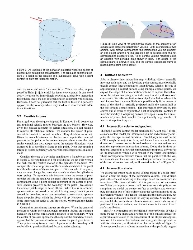
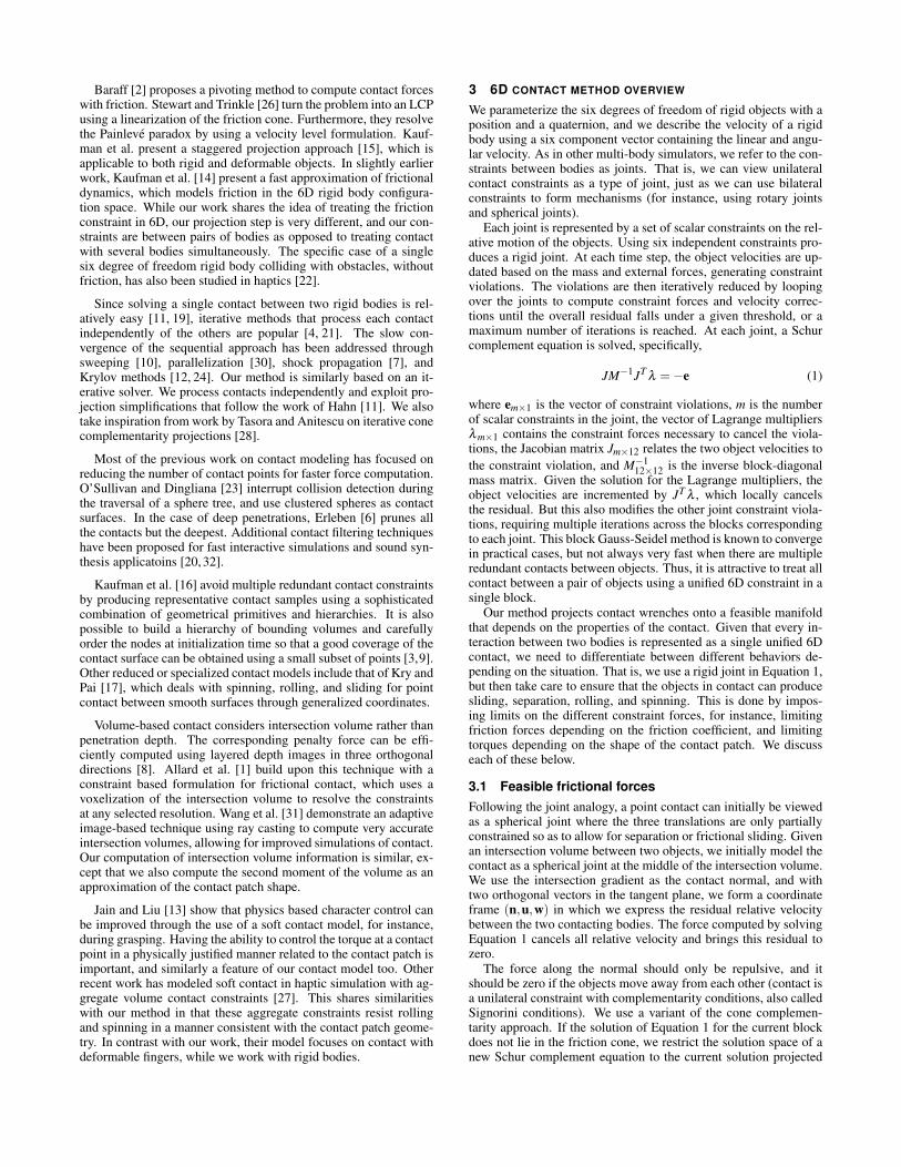
Figure 2: An example of the behavior expected when the center ofpressure d is outside the contact patch. The projected center of pres-sure p is used as the location of a subsequent solve with a pointcontact to allow for rotational motion.

onto the cone, and solve for a new force. This extra solve, as pro-posed by Hahn [11], is useful for faster convergence. It can avoidcostly iterations by immediately providing a plausible interactionforce that respects the non-interpenetration constraint while sliding.However, it does not guarantee that the friction force will perfectlyoppose the slip velocity, which may need to be resolved with addi-tional iterations.

3.2 Feasible torques

For a rigid joint, the torque computed in Equation 1 will counteractany rotational relative motion between the two bodies. However,given the contact geometry of certain situations, it is not realisticto remove all rotational motion. We monitor the center of pres-sure of the contact to evaluate whether rolling should occur or not.Given the wrench between two bodies, we compute the center ofpressure as the point on the contact tangent plane where the con-straint wrench has zero torque about the tangent directions whenexpressed in a coordinate frame at this point. Note that spinningtorque is treated separately and we will come back to this in a mo-ment.

Consider the case of a cylinder standing on a flat table as shownin Figure 2. Solving Equation 1 for a rigid joint, we get a 6D wrenchthat will zero the relative motion of the cylinder to the table. Wecompute the center of pressure of the wrench and check if the pointis within the extent of the contact patch. If it is outside of the patch,then we must change the constraint wrench to allow the cylinder tostart tipping. To reproduce this behavior when the center of pres-sure lies outside the patch, we do a new solve with a modified Schurcomplement using a point contact constraint at the center of pres-sure location projected to the boundary of the patch. We assumethe contact patch shape to be an ellipse. When this is an accurateapproximation, we avoid the need of having many contact pointsaround the boundary, as we can instead use a projection to approx-imate the point about which the object will tip. However, there aresome important subtleties to this projection. We present the detailsin Section 5.

Constraints on spinning torques are simpler. When the center ofpressure is within the contact patch, spinning torques are clampedbased on the normal force and the distance to the boundary. Whenthe center of pressure approaches the edge of the boundary, we rec-ognize that the pressure distribution across the patch goes to zero.Thus, points away from a center of pressure at the boundary willnot be able to provide frictional forces to resist spinning.

Figure 3: Side view of the geometrical model of the contact for anexaggerated large interpenetration volume. Left: intersection of twoobjects, with arrows representing the intersection volume gradienton one object, and the normal direction set to be parallel to the netcorresponding pressure force. Right: contact volume modeled usingan ellipsoid with principal axes shown in blue. The ellipse in thecontact plane is shown in red, and the contact coordinate frame isplaced at the point in the center.

4 CONTACT GEOMETRY

After a discrete-time integration step, colliding objects generallyintersect each other and the idealized point contact model typicallyused in contact force computation is not directly suitable. Instead ofapproximating a contact surface using multiple contact points, weexploit the shape of the intersection volume to capture the behav-ior of the interaction using a unified contact model with rotationalconstraints. We take inspiration from biped simulation, where it iswell known that static equilibrium is possible only if the center ofmass of the biped is vertically projected inside the convex hull ofthe foot-ground contact points. The information provided by thisconvex hull is easier to exploit than a set of independent contacts toinfer the stability. Computing convex envelopes is easy for a smallnumber of points, but complex for a potentially large number ofintersection points in space.

4.1 Intersection volume and gradientThe mono-volume contact model discussed by Allard et al. [1] cre-ates one contact model per intersection volume and efficiently com-putes the average normal direction. Parallel rays are cast on theGPU through the object surfaces, and for each ray, a simple one-dimensional intersection test is used to detect crossings and to com-pute the approximate intersection volume. Doing this in three or-thogonal directions allows the computation of the partial derivativesof the intersection volume with respect to the vertex coordinates.These correspond to pressure forces that are parallel with the ver-tex normals, and their net sum on each object defines the directionof the overall contact normal, as illustrated in the left of Figure 3.

4.2 Intersection shapeWe extend the image-based mono-volume model to collect infor-mation about the shape of the intersection volume. The difficultpart is the efficient modeling of the shape based on ray-surface in-tersections. The points identified in this process are too numerousto efficiently compute a convex hull. We thus use a simplifying as-sumption: we model the contact surface as a ellipse, and we com-pute the major axis of this ellipse using the second moment of theintersection volume. This tensor is much like the inertia tensor, butin this case it does not account for varying density. Since the raysare parallel, the intersection volumes associated with each ray are apartition of the total volume, and the net tensor is the sum of eachray’s contribution.

This 3×3 symmetric positive definite tensor provides us with abasic model of the shape and orientation of the contact surface. Itseigenvalues are related to the dimensions of the ellipsoidal approx-imation of the intersection volume, and its eigenvectors provide uswith its orientation, as illustrated in blue in the right of Figure 3.As we approach a zero volume intersection with a perfectly tangent

contact between flat surfaces, one eigenvector will be parallel tothe normal and the corresponding eigenvalue will be equal to thesum of the other two (see Appendix A). The two other directionsprovide us with an ellipse-shaped model of the contact area. In thegeneral case, after a time integration step, the contact volume is nei-ther zero nor flat and the ellipsoid may not be perfectly aligned withthe normal. In this case, we project the ellipsoid to a flat ellipse inthe tangent plane defined by the contact normal. Note that it is al-ways the linear component of the intersection volume gradient thatwe use as the normal.

5 CONTACT FORCE AND TORQUE

We use a rigid joint with six scalar constraints to compute the firstguess of the contact wrench. This is equivalent to assuming a stick-ing contact with no relative rolling or spinning motion. We solveEquation 1 with six scalar constraints expressed in the coordinateframe at the center of the intersection volume (as described in Sec-tion 3.1). The result is a wrench that contains both a 3D force and a3D torque. Given this solution, we may need to further modify theforce and torque to satisfy our contact constraints.

5.1 Schur complement and adjoint matrices

Equation 1 represents the constraint of one contact at the center ofthe patch. During the projection process, we need to move the con-straints into another reference frame by reformulating the constraintequation. To do so, we compute the adjoint matrix, which is usedto transform the wrenches and velocities from one reference frameto another. For example, the adjoint that transforms velocity from aworld frame to a contact frame is written

Adcw =

[Rc

w p Rcw

0 Rcw

](2)

where Rcw is the rotation matrix, p is the translation, and ˆ de-

notes the cross product operator. To transform velocities from oneframe to another we multiply by the adjoint, whereas to transformwrenches, we use the inverse transpose of Adc

w . Note that when us-ing the adjoint defined above, the wrench and velocity vectors havetheir linear quantities in the top three components, and rotationalquantities in the bottom three.

Given the Schur complement block for a contact expressed incoordinates of the world frame, we can easily produce an equivalentconstraint problem in different coordinates by multiplying on bothsides. That is,

Adcw JM−1JT Adc T

w λ c =− Adcw e (3)

is equivalent to Equation 1, except that the solution is now ex-pressed in a contact reference frame. Writing the problem or thesolution in different frames is useful as we can easily monitor im-portant quantities, such as tangential sliding, or make simple modi-fications to the system, for instance, to remove a rolling constraint.

5.2 Cone projection

The contact force is decomposed into a repulsion force fn parallelto the normal and a tangential force ft in the tangent plane. It isprojected to the Coulomb cone centered on the normal, as presentedin Section 3.1. If the force is outside the Coulomb cone, we rewriteEquation 1 by constraining the linear component of the spatial forceto be in the direction of the Coulomb cone projection while keepingthe non-rolling assumptions of a rigid contact. We can write this as

RJM−1JT Qλ′ =−Re, (4)

where

Q =

[q 00 I

]∈ R6×4 , (5)

R =

[eT

1 00 I

]∈ R4×6, eT

1 = [1 0 0] . (6)

Here, I is a 3×3 identity matrix, and the column vector q in Equa-tion 5 is the direction of the force projected onto the cone. Aftersolving Equation 4, the wrench is recomputed as Qλ ′. Solving fornew values of torques is essential, as there is coupling between theforce and torque parts of the wrench.

An intuitive example that can be used to illustrate this is a spherelanding on an incline plane with zero friction. The sphere is ex-pected to land and slide without rolling. The initial force computedis directly opposing the gravity, and the computed torque opposesthe moment produced by this force. Given that there is no fric-tion, the cone of permissible forces is a ray in the normal direc-tion, and the linear force obtained by resolving the system will bealong the normal. But the wrench we initially computed included atorque that opposed the moment produced by the non-normal force(that is, the force was not pointing toward the center of mass of thesphere). If we were to keep the torque and only project the force,we would get a net moment around the center of the sphere, and thesphere will begin to roll. Since the center of the contact patch andthe center of mass of the sphere form a line parallel to the normal,the new solution will not produce any moment and the computedtorque will be zero. This observation is particularly important aswe use the torque to compute the location of the center of pressureas explained below.

5.3 Rolling torque and center of pressureIdentifying the center of pressure of a contact wrench is importantto determine if two objects will exhibit rolling behavior. The adjointinverse transpose can let us express wrenches in different coordi-nate frames, but we can also build intuition by looking at a simplerequation. Given a force f and a torque τc expressed at a point c, theequivalent wrench expressed at point p has the same linear force,and has the torque

τp = τc +(p− c)× f. (7)

We decompose the contact torque τ into a normal componentτn opposed to spinning, and a tangential component τt opposed torolling. The center of pressure (COP) is the point in the contactplane where the equivalent wrench has zero tangential torque. Wecan think of this as the location of the repulsion force. Given therolling torque τt = (τu,τw)

T in the contact frame, the COP is lo-cated at d = 1

fn(τw,−τu)

T , as illustrated in Figure 4.

5.4 Center of pressure projectionIf the COP lies inside the contact area modeled by the ellipticalcontact patch, the rolling torque is feasible and we leave it unmod-ified. Otherwise, it corresponds to a pressure distribution whichcan not be positive everywhere in the contact area, which violatesthe Signorini conditions. We thus clamp it to the closest edge, forexample, point p in Figure 4, and the resulting rolling torque be-comes fn× (p− c). This can be done with an iterative root findingalgorithm. A good solution can be found in 4 to 5 iterations.

We use a Euclidean distance metric in the projection, and ob-serve good behavior in practice. Nevertheless, for frictionless con-tact, we note that the projection should instead use a mass weightedmetric that takes into account the inertia of the two objects in con-tact. However, for frictional contact, there does not exist a simplemetric that will allow us to use projection to predict the center ofpressure location. Instead, we choose the simple Euclidean projec-tion and allow errors to be resolved through multiple iterations in

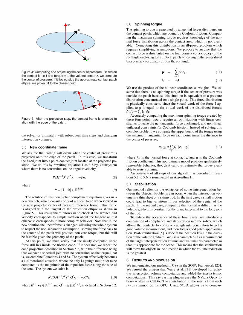
Figure 4: Computing and projecting the center of pressure. Based onthe contact force f and torque τ at the volume center c, we computethe center of pressure. If it lies outside the approximate contact patchellipse, we project it to the closest point.

Figure 5: After the projection step, the contact frame is oriented toalign with the edge of the patch.

the solver, or ultimately with subsequent time steps and changingintersection volumes.

5.5 New coordinate frame

We assume that rolling will occur when the center of pressure isprojected onto the edge of the patch. In this case, we transformthe fixed joint into a point-contact joint located at the projected po-sition. We do this by rewriting Equation 1 as a 3-by-3 subsystemwhere there is no constraints on the angular velocity,

PJM−1JT PTλ =−Pe, (8)

whereP =

[I 0

]∈ R3×6. (9)

The solution of this new Schur complement equation gives us anew wrench, which consists only of a linear force when viewed inthe new projected center of pressure reference frame. This frameis aligned with the tangent of the projection ellipse as shown inFigure 5. This realignment allows us to check if the wrench andvelocity corresponds to simple rotation about the tangent or if itotherwise corresponds to more complex behavior. Note that in thenew solution the linear force is changed, allowing the whole systemto respect the non-separation assumption. Moving the force back tothe center of the patch will produce non-zero torque, but this willbe feasible given the geometry of the patch.

At this point, we must verify that the newly computed linearforce still lies inside the friction cone. If it does not, we repeat thecone projection described in Section 5.2, with the difference beingthat we have a spherical joint with no constraints on the torque (thatis, we combine Equations 4 and 8). The system effectively becomesa 1-dimensional equation, where the only Lagrange multiplier to becomputed is the magnitude of the repulsion force along the side ofthe cone. The system we solve is

R′PJM−1JT PT Q′λ =−RPe, (10)

where R′ = e1 ∈R1×3 and Q′ = q∈R3×1, as defined in Section 5.2.

5.6 Spinning torqueThe spinning torque is generated by tangential forces distributed onthe contact patch, which are bound by Coulomb friction. Comput-ing the maximum spinning torque requires knowledge of the nor-mal force distribution across the contact area, which is not avail-able. Computing this distribution is an ill-posed problem whichrequires simplifying assumptions. We propose to assume that thecontact force is distributed on the four corners (c1,c2,c3,c4) of therectangle enclosing the elliptical patch according to the generalizedbarycentric coordinates of p in the rectangle,

p =4

∑i=1

wici, (11)

fi = wif. (12)

We use the product of the bilinear coordinates as weights. We as-sume that there is no spinning torque if the center of pressure wasoutside the patch because this situation is equivalent to a pressuredistribution concentrated on a single point. This force distributionis physically consistent, since the virtual work of the force f ap-plied to p is equal to the virtual work of the distributed forces:f ·dp = ∑i fi ·dci.

Accurately computing the maximum spinning torque created bythese four points would require an optimization with linear con-straints to leave the net tangential force unchanged, and non-linearunilateral constraints for Coulomb friction. Instead of solving thiscomplex problem, we compute the upper bound of the torque usingthe maximum tangential force on each point times the distance tothe center of pressure,

τp ≤ µ ∑i

fni‖ci−p‖ (13)

where fni is the normal force at contact ci and µ is the Coulombfriction coefficient. This approximate model provides qualitativelyreasonable behavior, though it can over estimate the torque avail-able to resist spinning.

An overview of all steps of our algorithm as described in Sec-tions 5.1 to 5.6 is summarized in Algorithm 1.

5.7 StabilizationOur method relies on the existence of some interpenetration be-tween the objects. Problems can occur when the intersection vol-ume is a thin sheet or a skinny rod. In the first case, a small motioncould lead to big variations in our selection of the center of thepatch. In the second case, computing the normal is difficult as thevolume gradient is constant for the plane tangential to the long axisof the rod.

To reduce the occurrence of these limit cases, we introduce acombination of compliance and stabilization into the solver, whichallows the contacts to conserve enough interpenetration to get agood volume measurement, and therefore a good patch approxima-tion. Post-stabilization [5] is done at the position level in the direc-tion of the volume gradient. We use a parameter e as a measurementof the target interpenetration volume and we tune this parameter sothat it is appropriate for the scene. This means that the stabilizationwill move the objects in the direction in which the volume reductionis the greatest.

6 RESULTS AND DISCUSSION

We implemented our method in C++ in the SOFA Framework [25].We reused the plug-in that Wang et al. [31] developed for adap-tive intersection volume computation and added the inertia tensorcomputations. This ray casting plug-in uses the NVidia Optix li-brary written in CUDA. The contribution to the inertia from eachray is summed on the GPU. Using SOFA allows us to compare

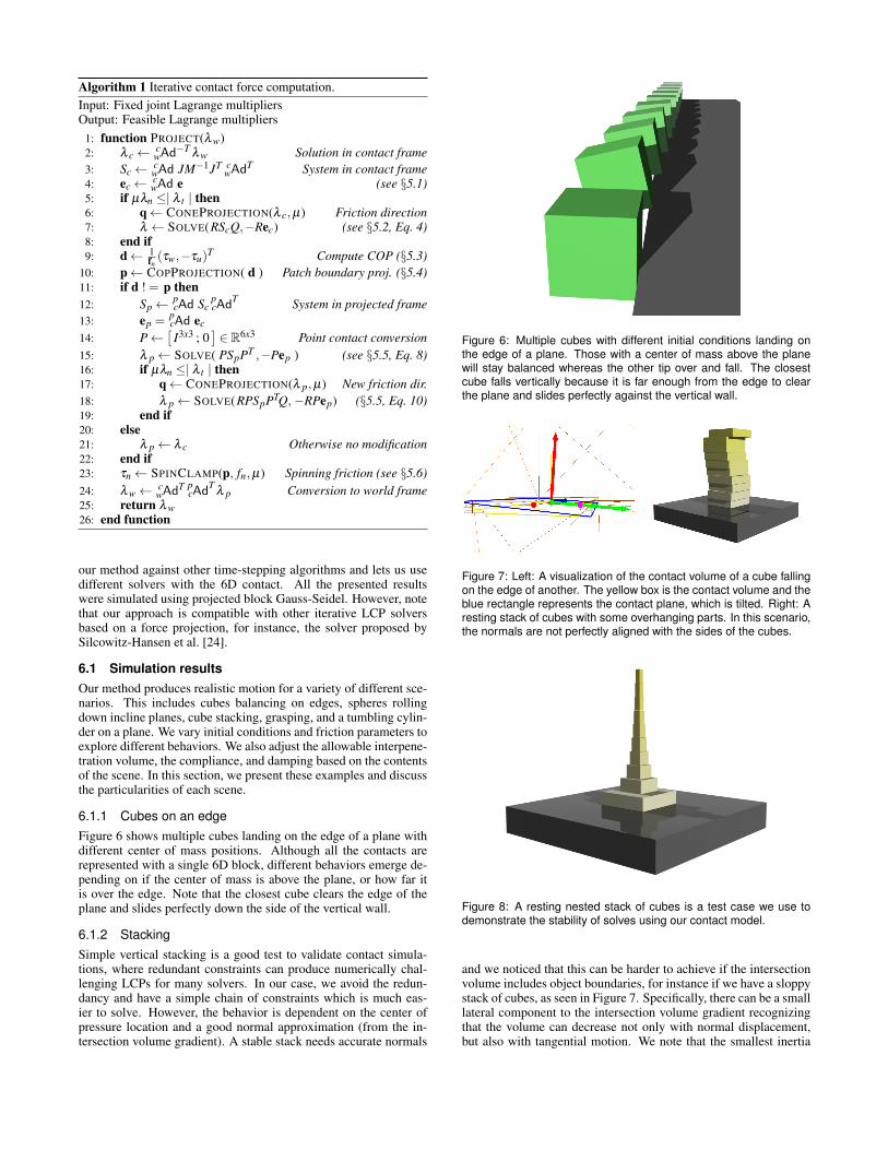
Algorithm 1 Iterative contact force computation.Input: Fixed joint Lagrange multipliersOutput: Feasible Lagrange multipliers

1: function PROJECT(λ w)2: λ c← Adc −T

w λ w Solution in contact frame3: Sc← Adc

w JM−1JT Adc Tw System in contact frame

4: ec← Adcw e (see §5.1)

5: if µλn ≤| λ t | then6: q← CONEPROJECTION(λ c,µ) Friction direction7: λ ← SOLVE(RScQ,−Rec) (see §5.2, Eq. 4)8: end if9: d← 1

fn(τw,−τu)

T Compute COP (§5.3)10: p← COPPROJECTION( d ) Patch boundary proj. (§5.4)11: if d ! = p then12: Sp← Adp

c Sc Adp Tc System in projected frame

13: ep = Adpc ec

14: P←[

I3x3 ; 0]∈ R6x3 Point contact conversion

15: λ p← SOLVE( PSpPT ,−Pep ) (see §5.5, Eq. 8)16: if µλn ≤| λ t | then17: q← CONEPROJECTION(λ p,µ) New friction dir.18: λ p← SOLVE(RPSpPTQ,−RPep) (§5.5, Eq. 10)19: end if20: else21: λ p← λ c Otherwise no modification22: end if23: τn← SPINCLAMP(p, fn,µ) Spinning friction (see §5.6)24: λ w← Adc T

w Adp Tc λ p Conversion to world frame

25: return λ w26: end function

our method against other time-stepping algorithms and lets us usedifferent solvers with the 6D contact. All the presented resultswere simulated using projected block Gauss-Seidel. However, notethat our approach is compatible with other iterative LCP solversbased on a force projection, for instance, the solver proposed bySilcowitz-Hansen et al. [24].

6.1 Simulation resultsOur method produces realistic motion for a variety of different sce-narios. This includes cubes balancing on edges, spheres rollingdown incline planes, cube stacking, grasping, and a tumbling cylin-der on a plane. We vary initial conditions and friction parameters toexplore different behaviors. We also adjust the allowable interpene-tration volume, the compliance, and damping based on the contentsof the scene. In this section, we present these examples and discussthe particularities of each scene.

6.1.1 Cubes on an edgeFigure 6 shows multiple cubes landing on the edge of a plane withdifferent center of mass positions. Although all the contacts arerepresented with a single 6D block, different behaviors emerge de-pending on if the center of mass is above the plane, or how far itis over the edge. Note that the closest cube clears the edge of theplane and slides perfectly down the side of the vertical wall.

6.1.2 StackingSimple vertical stacking is a good test to validate contact simula-tions, where redundant constraints can produce numerically chal-lenging LCPs for many solvers. In our case, we avoid the redun-dancy and have a simple chain of constraints which is much eas-ier to solve. However, the behavior is dependent on the center ofpressure location and a good normal approximation (from the in-tersection volume gradient). A stable stack needs accurate normals

Figure 6: Multiple cubes with different initial conditions landing onthe edge of a plane. Those with a center of mass above the planewill stay balanced whereas the other tip over and fall. The closestcube falls vertically because it is far enough from the edge to clearthe plane and slides perfectly against the vertical wall.

Figure 7: Left: A visualization of the contact volume of a cube fallingon the edge of another. The yellow box is the contact volume and theblue rectangle represents the contact plane, which is tilted. Right: Aresting stack of cubes with some overhanging parts. In this scenario,the normals are not perfectly aligned with the sides of the cubes.

Figure 8: A resting nested stack of cubes is a test case we use todemonstrate the stability of solves using our contact model.

and we noticed that this can be harder to achieve if the intersectionvolume includes object boundaries, for instance if we have a sloppystack of cubes, as seen in Figure 7. Specifically, there can be a smalllateral component to the intersection volume gradient recognizingthat the volume can decrease not only with normal displacement,but also with tangential motion. We note that the smallest inertia

direction corresponds to what we would consider the true normal tothe surface, but the intersection gradient is typically close enoughso as not to cause problems provided there is some friction in thesystem. Thus, the stack in Figure 8, specifically avoids this issuethrough the use of a tapered stack shape. In contrast, we exploredlow friction settings with a cube dropped from a small height nearthe edge of another. While the intersection volume and gradient(i.e., the contact normal) depend on the relative velocity and timestep, for this test we observe sliding artifacts only when the frictioncoefficient is below 0.031 (see left of Figure 7 and the supplemen-tary video).

In the future, we could use a heuristic to choose between thevolume gradient and the smallest inertia direction for our normal,or use a blended combination of the two.

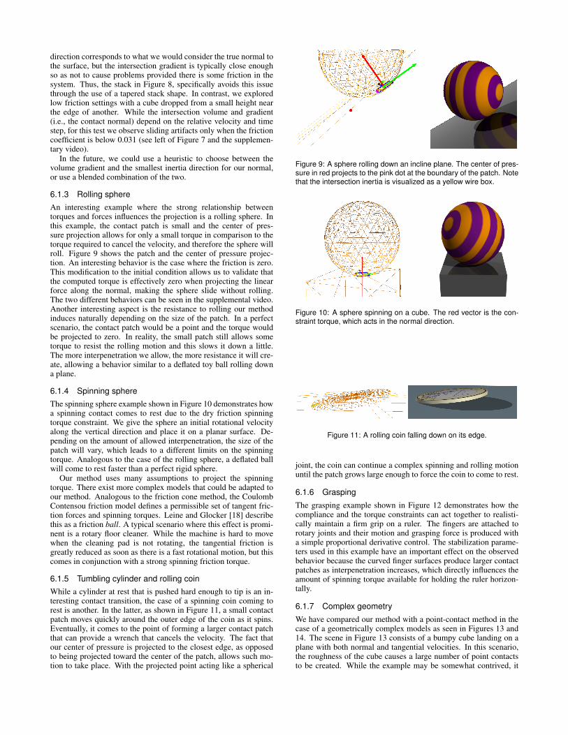
6.1.3 Rolling sphereAn interesting example where the strong relationship betweentorques and forces influences the projection is a rolling sphere. Inthis example, the contact patch is small and the center of pres-sure projection allows for only a small torque in comparison to thetorque required to cancel the velocity, and therefore the sphere willroll. Figure 9 shows the patch and the center of pressure projec-tion. An interesting behavior is the case where the friction is zero.This modification to the initial condition allows us to validate thatthe computed torque is effectively zero when projecting the linearforce along the normal, making the sphere slide without rolling.The two different behaviors can be seen in the supplemental video.Another interesting aspect is the resistance to rolling our methodinduces naturally depending on the size of the patch. In a perfectscenario, the contact patch would be a point and the torque wouldbe projected to zero. In reality, the small patch still allows sometorque to resist the rolling motion and this slows it down a little.The more interpenetration we allow, the more resistance it will cre-ate, allowing a behavior similar to a deflated toy ball rolling downa plane.

6.1.4 Spinning sphereThe spinning sphere example shown in Figure 10 demonstrates howa spinning contact comes to rest due to the dry friction spinningtorque constraint. We give the sphere an initial rotational velocityalong the vertical direction and place it on a planar surface. De-pending on the amount of allowed interpenetration, the size of thepatch will vary, which leads to a different limits on the spinningtorque. Analogous to the case of the rolling sphere, a deflated ballwill come to rest faster than a perfect rigid sphere.

Our method uses many assumptions to project the spinningtorque. There exist more complex models that could be adapted toour method. Analogous to the friction cone method, the CoulombContensou friction model defines a permissible set of tangent fric-tion forces and spinning torques. Leine and Glocker [18] describethis as a friction ball. A typical scenario where this effect is promi-nent is a rotary floor cleaner. While the machine is hard to movewhen the cleaning pad is not rotating, the tangential friction isgreatly reduced as soon as there is a fast rotational motion, but thiscomes in conjunction with a strong spinning friction torque.

6.1.5 Tumbling cylinder and rolling coinWhile a cylinder at rest that is pushed hard enough to tip is an in-teresting contact transition, the case of a spinning coin coming torest is another. In the latter, as shown in Figure 11, a small contactpatch moves quickly around the outer edge of the coin as it spins.Eventually, it comes to the point of forming a larger contact patchthat can provide a wrench that cancels the velocity. The fact thatour center of pressure is projected to the closest edge, as opposedto being projected toward the center of the patch, allows such mo-tion to take place. With the projected point acting like a spherical

Figure 9: A sphere rolling down an incline plane. The center of pres-sure in red projects to the pink dot at the boundary of the patch. Notethat the intersection inertia is visualized as a yellow wire box.

Figure 10: A sphere spinning on a cube. The red vector is the con-straint torque, which acts in the normal direction.

Figure 11: A rolling coin falling down on its edge.

joint, the coin can continue a complex spinning and rolling motionuntil the patch grows large enough to force the coin to come to rest.

6.1.6 Grasping

The grasping example shown in Figure 12 demonstrates how thecompliance and the torque constraints can act together to realisti-cally maintain a firm grip on a ruler. The fingers are attached torotary joints and their motion and grasping force is produced witha simple proportional derivative control. The stabilization parame-ters used in this example have an important effect on the observedbehavior because the curved finger surfaces produce larger contactpatches as interpenetration increases, which directly influences theamount of spinning torque available for holding the ruler horizon-tally.

6.1.7 Complex geometry

We have compared our method with a point-contact method in thecase of a geometrically complex models as seen in Figures 13 and14. The scene in Figure 13 consists of a bumpy cube landing on aplane with both normal and tangential velocities. In this scenario,the roughness of the cube causes a large number of point contactsto be created. While the example may be somewhat contrived, it

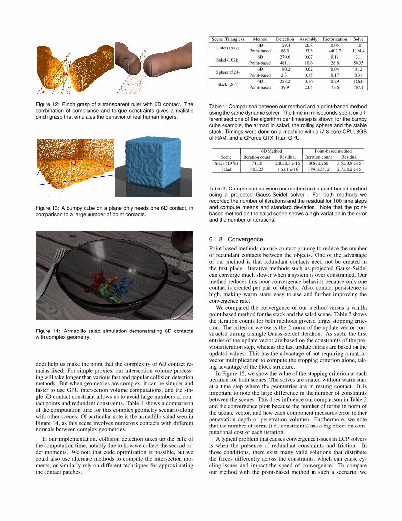
Figure 12: Pinch grasp of a transparent ruler with 6D contact. Thecombination of compliance and torque constraints gives a realisticpinch grasp that emulates the behavior of real human fingers.

Figure 13: A bumpy cube on a plane only needs one 6D contact, incomparison to a large number of point contacts.

Figure 14: Armadillo salad simulation demonstrating 6D contactswith complex geometry.

does help us make the point that the complexity of 6D contact re-mains fixed. For simple proxies, our intersection volume process-ing will take longer than various fast and popular collision detectionmethods. But when geometries are complex, it can be simpler andfaster to use GPU intersection volume computations, and the sin-gle 6D contact constraint allows us to avoid large numbers of con-tact points and redundant constraints. Table 1 shows a comparisonof the computation time for this complex geometry scenario alongwith other scenes. Of particular note is the armadillo salad seen inFigure 14, as this scene involves numerous contacts with differentnormals between complex geometries.

In our implementation, collision detection takes up the bulk ofthe computation time, notably due to how we collect the second or-der moments. We note that code optimization is possible, but wecould also use alternate methods to compute the intersection mo-ments, or similarly rely on different techniques for approximatingthe contact patches.

Scene (Triangles) Method Detection Assembly Factorization Solve

Cube (197k)6D 129.4 26.8 0.05 1.0

Point-based 86.3 93.3 4402.7 1194.4

Salad (102k)6D 270.6 0.07 0.11 3.1

Point-based 481.1 10.6 28.8 50.35

Sphere (524)6D 180.2 0.02 0.04 0.12

Point-based 2.31 0.15 0.17 0.31

Stack (264)6D 228.2 0.16 0.29 186.0

Point-based 39.9 2.04 7.36 407.1

Table 1: Comparison between our method and a point-based methodusing the same dynamic solver. The time in milliseconds spent on dif-ferent sections of the algorithm per timestep is shown for the bumpycube example, the armadillo salad, the rolling sphere and the stablestack. Timings were done on a machine with a i7 8-core CPU, 8GBof RAM, and a GForce GTX Titan GPU.

6D Method Point-based methodScene Iteration count Residual Iteration count Residual

Stack (197k) 74±0 2.8±0.3 e-16 3087±260 3.5±0.8 e-15Salad 40±23 1.6±1 e-16 1796±3512 2.7±8.2 e-15

Table 2: Comparison between our method and a point-based methodusing a projected Gauss-Seidel solver. For both methods werecorded the number of iterations and the residual for 100 time stepsand compute means and standard deviation. Note that the point-based method on the salad scene shows a high variation in the errorand the number of iterations.

6.1.8 ConvergencePoint-based methods can use contact pruning to reduce the numberof redundant contacts between the objects. One of the advantageof our method is that redundant contacts need not be created inthe first place. Iterative methods such as projected Gauss-Seidelcan converge much slower when a system is over constrained. Ourmethod reduces this poor convergence behavior because only onecontact is created per pair of objects. Also, contact persistence ishigh, making warm starts easy to use and further improving theconvergence rate.

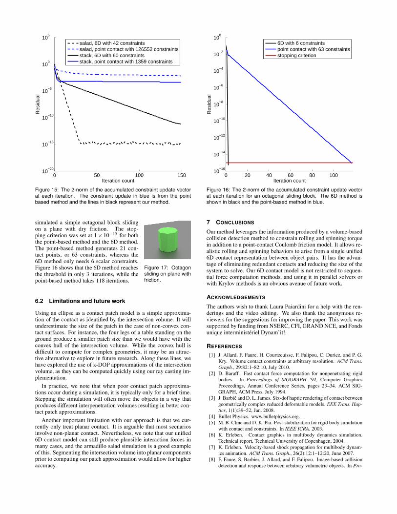
We compared the convergence of our method versus a vanillapoint-based method for the stack and the salad scene. Table 2 showsthe iteration counts for both methods given a target stopping crite-rion. The criterion we use is the 2-norm of the update vector con-structed during a single Gauss-Seidel iteration. As such, the firstentries of the update vector are based on the constraints of the pre-vious iteration step, whereas the last update entries are based on theupdated values. This has the advantage of not requiring a matrix-vector multiplication to compute the stopping criterion alone, tak-ing advantage of the block structure.

In Figure 15, we show the value of the stopping criterion at eachiteration for both scenes. The solves are started without warm startat a time step where the geometries are in resting contact. It isimportant to note the large difference in the number of constraintsbetween the scenes. This does influence our comparison in Table 2and the convergence plots because the number of terms in norm ofthe update vector, and how each component measures error (eitherpenetration depth or penetration volume). Furthermore, we notethat the number of terms (i.e., constraints) has a big effect on com-putational cost of each iteration.

A typical problem that causes convergence issues in LCP solversis when the presence of redundant constraints and friction. Inthose conditions, there exist many valid solutions that distributethe forces differently across the constraints, which can cause cy-cling issues and impact the speed of convergence. To compareour method with the point-based method in such a scenario, we

0 50 100 15010

−20

10−15

10−10

10−5

100

105

Iteration count

Res

idua

l

salad, 6D with 42 constraintssalad, point contact with 126552 constraintsstack, 6D with 60 constraintsstack, point contact with 1359 constraints

Figure 15: The 2-norm of the accumulated constraint update vectorat each iteration. The constraint update in blue is from the pointbased method and the lines in black represent our method.

0 20 40 60 80 10010

−16

10−14

10−12

10−10

10−8

10−6

10−4

10−2

100

Iteration count

Res

idua

l

6D with 6 constraintspoint contact with 63 constraintsstopping criterion

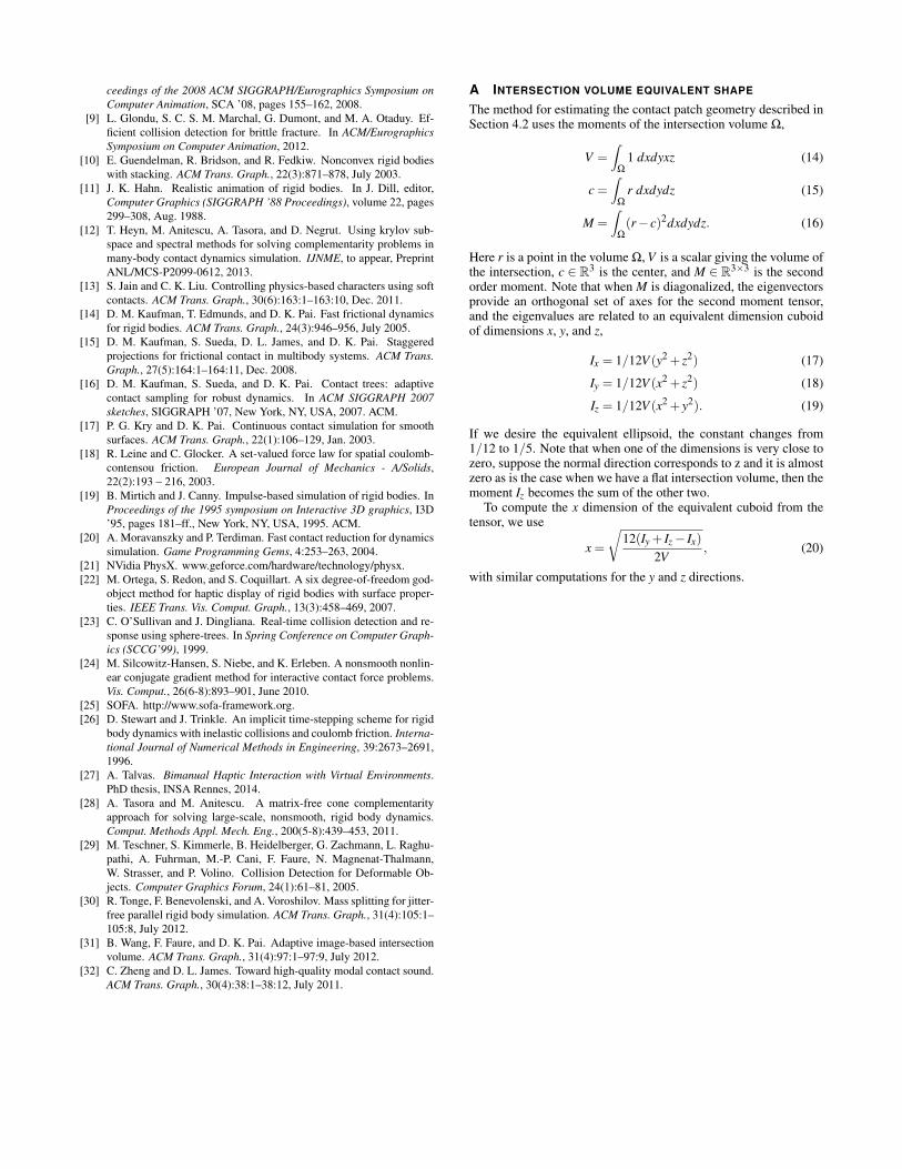
Figure 16: The 2-norm of the accumulated constraint update vectorat each iteration for an octagonal sliding block. The 6D method isshown in black and the point-based method in blue.

Figure 17: Octagonsliding on plane withfriction.

simulated a simple octagonal block slidingon a plane with dry friction. The stop-ping criterion was set at 1× 10−15 for boththe point-based method and the 6D method.The point-based method generates 21 con-tact points, or 63 constraints, whereas the6D method only needs 6 scalar constraints.Figure 16 shows that the 6D method reachesthe threshold in only 3 iterations, while thepoint-based method takes 118 iterations.

6.2 Limitations and future work

Using an ellipse as a contact patch model is a simple approxima-tion of the contact as identified by the intersection volume. It willunderestimate the size of the patch in the case of non-convex con-tact surfaces. For instance, the four legs of a table standing on theground produce a smaller patch size than we would have with theconvex hull of the intersection volume. While the convex hull isdifficult to compute for complex geometries, it may be an attrac-tive alternative to explore in future research. Along these lines, wehave explored the use of k-DOP approximations of the intersectionvolume, as they can be computed quickly using our ray casting im-plementation.

In practice, we note that when poor contact patch approxima-tions occur during a simulation, it is typically only for a brief time.Stepping the simulation will often move the objects in a way thatproduces different interpenetration volumes resulting in better con-tact patch approximations.

Another important limitation with our approach is that we cur-rently only treat planar contact. It is arguable that most scenariosinvolve non-planar contact. Nevertheless, we note that our unified6D contact model can still produce plausible interaction forces inmany cases, and the armadillo salad simulation is a good exampleof this. Segmenting the intersection volume into planar componentsprior to computing our patch approximation would allow for higheraccuracy.

7 CONCLUSIONS

Our method leverages the information produced by a volume-basedcollision detection method to constrain rolling and spinning torquein addition to a point-contact Coulomb friction model. It allows re-alistic rolling and spinning behaviors to arise from a single unified6D contact representation between object pairs. It has the advan-tage of eliminating redundant contacts and reducing the size of thesystem to solve. Our 6D contact model is not restricted to sequen-tial force computation methods, and using it in parallel solvers orwith Krylov methods is an obvious avenue of future work.

ACKNOWLEDGEMENTS

The authors wish to thank Laura Paiardini for a help with the ren-derings and the video editing. We also thank the anonymous re-viewers for the suggestions for improving the paper. This work wassupported by funding from NSERC, CFI, GRAND NCE, and Fondsunique interministeriel Dynam’it!.

REFERENCES

[1] J. Allard, F. Faure, H. Courtecuisse, F. Falipou, C. Duriez, and P. G.Kry. Volume contact constraints at arbitrary resolution. ACM Trans.Graph., 29:82:1–82:10, July 2010.

[2] D. Baraff. Fast contact force computation for nonpenetrating rigidbodies. In Proceedings of SIGGRAPH ’94, Computer GraphicsProceedings, Annual Conference Series, pages 23–34. ACM SIG-GRAPH, ACM Press, July 1994.

[3] J. Barbic and D. L. James. Six-dof haptic rendering of contact betweengeometrically complex reduced deformable models. EEE Trans. Hap-tics, 1(1):39–52, Jan. 2008.

[4] Bullet Physics. www.bulletphysics.org.[5] M. B. Cline and D. K. Pai. Post-stabilization for rigid body simulation

with contact and constraints. In IEEE ICRA, 2003.[6] K. Erleben. Contact graphics in multibody dynamics simulation.

Technical report, Technical University of Copenhagen, 2004.[7] K. Erleben. Velocity-based shock propagation for multibody dynam-

ics animation. ACM Trans. Graph., 26(2):12:1–12:20, June 2007.[8] F. Faure, S. Barbier, J. Allard, and F. Falipou. Image-based collision

detection and response between arbitrary volumetric objects. In Pro-

ceedings of the 2008 ACM SIGGRAPH/Eurographics Symposium onComputer Animation, SCA ’08, pages 155–162, 2008.

[9] L. Glondu, S. C. S. M. Marchal, G. Dumont, and M. A. Otaduy. Ef-ficient collision detection for brittle fracture. In ACM/EurographicsSymposium on Computer Animation, 2012.

[10] E. Guendelman, R. Bridson, and R. Fedkiw. Nonconvex rigid bodieswith stacking. ACM Trans. Graph., 22(3):871–878, July 2003.

[11] J. K. Hahn. Realistic animation of rigid bodies. In J. Dill, editor,Computer Graphics (SIGGRAPH ’88 Proceedings), volume 22, pages299–308, Aug. 1988.

[12] T. Heyn, M. Anitescu, A. Tasora, and D. Negrut. Using krylov sub-space and spectral methods for solving complementarity problems inmany-body contact dynamics simulation. IJNME, to appear, PreprintANL/MCS-P2099-0612, 2013.

[13] S. Jain and C. K. Liu. Controlling physics-based characters using softcontacts. ACM Trans. Graph., 30(6):163:1–163:10, Dec. 2011.

[14] D. M. Kaufman, T. Edmunds, and D. K. Pai. Fast frictional dynamicsfor rigid bodies. ACM Trans. Graph., 24(3):946–956, July 2005.

[15] D. M. Kaufman, S. Sueda, D. L. James, and D. K. Pai. Staggeredprojections for frictional contact in multibody systems. ACM Trans.Graph., 27(5):164:1–164:11, Dec. 2008.

[16] D. M. Kaufman, S. Sueda, and D. K. Pai. Contact trees: adaptivecontact sampling for robust dynamics. In ACM SIGGRAPH 2007sketches, SIGGRAPH ’07, New York, NY, USA, 2007. ACM.

[17] P. G. Kry and D. K. Pai. Continuous contact simulation for smoothsurfaces. ACM Trans. Graph., 22(1):106–129, Jan. 2003.

[18] R. Leine and C. Glocker. A set-valued force law for spatial coulomb-contensou friction. European Journal of Mechanics - A/Solids,22(2):193 – 216, 2003.

[19] B. Mirtich and J. Canny. Impulse-based simulation of rigid bodies. InProceedings of the 1995 symposium on Interactive 3D graphics, I3D’95, pages 181–ff., New York, NY, USA, 1995. ACM.

[20] A. Moravanszky and P. Terdiman. Fast contact reduction for dynamicssimulation. Game Programming Gems, 4:253–263, 2004.

[21] NVidia PhysX. www.geforce.com/hardware/technology/physx.[22] M. Ortega, S. Redon, and S. Coquillart. A six degree-of-freedom god-

object method for haptic display of rigid bodies with surface proper-ties. IEEE Trans. Vis. Comput. Graph., 13(3):458–469, 2007.

[23] C. O’Sullivan and J. Dingliana. Real-time collision detection and re-sponse using sphere-trees. In Spring Conference on Computer Graph-ics (SCCG’99), 1999.

[24] M. Silcowitz-Hansen, S. Niebe, and K. Erleben. A nonsmooth nonlin-ear conjugate gradient method for interactive contact force problems.Vis. Comput., 26(6-8):893–901, June 2010.

[25] SOFA. http://www.sofa-framework.org.[26] D. Stewart and J. Trinkle. An implicit time-stepping scheme for rigid

body dynamics with inelastic collisions and coulomb friction. Interna-tional Journal of Numerical Methods in Engineering, 39:2673–2691,1996.

[27] A. Talvas. Bimanual Haptic Interaction with Virtual Environments.PhD thesis, INSA Rennes, 2014.

[28] A. Tasora and M. Anitescu. A matrix-free cone complementarityapproach for solving large-scale, nonsmooth, rigid body dynamics.Comput. Methods Appl. Mech. Eng., 200(5-8):439–453, 2011.

[29] M. Teschner, S. Kimmerle, B. Heidelberger, G. Zachmann, L. Raghu-pathi, A. Fuhrman, M.-P. Cani, F. Faure, N. Magnenat-Thalmann,W. Strasser, and P. Volino. Collision Detection for Deformable Ob-jects. Computer Graphics Forum, 24(1):61–81, 2005.

[30] R. Tonge, F. Benevolenski, and A. Voroshilov. Mass splitting for jitter-free parallel rigid body simulation. ACM Trans. Graph., 31(4):105:1–105:8, July 2012.

[31] B. Wang, F. Faure, and D. K. Pai. Adaptive image-based intersectionvolume. ACM Trans. Graph., 31(4):97:1–97:9, July 2012.

[32] C. Zheng and D. L. James. Toward high-quality modal contact sound.ACM Trans. Graph., 30(4):38:1–38:12, July 2011.

A INTERSECTION VOLUME EQUIVALENT SHAPE

The method for estimating the contact patch geometry described inSection 4.2 uses the moments of the intersection volume Ω,

V =∫

Ω

1 dxdyxz (14)

c =∫

Ω

r dxdydz (15)

M =∫

Ω

(r− c)2dxdydz. (16)

Here r is a point in the volume Ω, V is a scalar giving the volume ofthe intersection, c ∈ R3 is the center, and M ∈ R3×3 is the secondorder moment. Note that when M is diagonalized, the eigenvectorsprovide an orthogonal set of axes for the second moment tensor,and the eigenvalues are related to an equivalent dimension cuboidof dimensions x, y, and z,

Ix = 1/12V (y2 + z2) (17)

Iy = 1/12V (x2 + z2) (18)

Iz = 1/12V (x2 + y2). (19)

If we desire the equivalent ellipsoid, the constant changes from1/12 to 1/5. Note that when one of the dimensions is very close tozero, suppose the normal direction corresponds to z and it is almostzero as is the case when we have a flat intersection volume, then themoment Iz becomes the sum of the other two.

To compute the x dimension of the equivalent cuboid from thetensor, we use

x =

√12(Iy + Iz− Ix)

2V, (20)

with similar computations for the y and z directions.