7-6

Chapter 5

5.1 .) ~ "

(i60) ; s" (-i-:/3

-i:13).

f2 = 1 SO/ll = 13.64

b) T2 is 3ri,2 (see (5-5))

c) HO :~. ~ (7,11)

a =- .05 so F2,2(.05~ - 19.00

Since T2 _ 13.64 (;' 3FZ,2(.05) = 3(19) =57; do not reject H1l at

the a - .05 1 eve1

5.3 a) TZ ;.

n

(n-1)!.J.g1 (:j-~O)(:j-~O)'!

n ,- - (n-1) = 3(~4) - 3 = 13:64! r (x.-i)(xJ.-i)'! .j=l -J - - -

b) li - (I Jïi (~j-~)(~j-~) 'I 'r =

- I j~i (~r~~H~j-~o)' i/

Wil ks i 1 ambda '" A2/n = A1/Z = '.0325 - .1803

(44)2244 =.0325

5.5 HO:~' = (.'5'5,;60); TZ = 1.17

a -.05; FZ ,40( .05) ;. 3.23

Since TZ '" 1.17 (; 2~~) F2,40( .05) =- 2.05(3.23) = 6.62,

we do not reject HO at the a" .05 level. The r,esult is ~onsistent

with the 9Si confidence ellipse for ~ pi~tured in Figure 5.1 since

\11 = (.'55,.60) is inside the ellipse.-

77

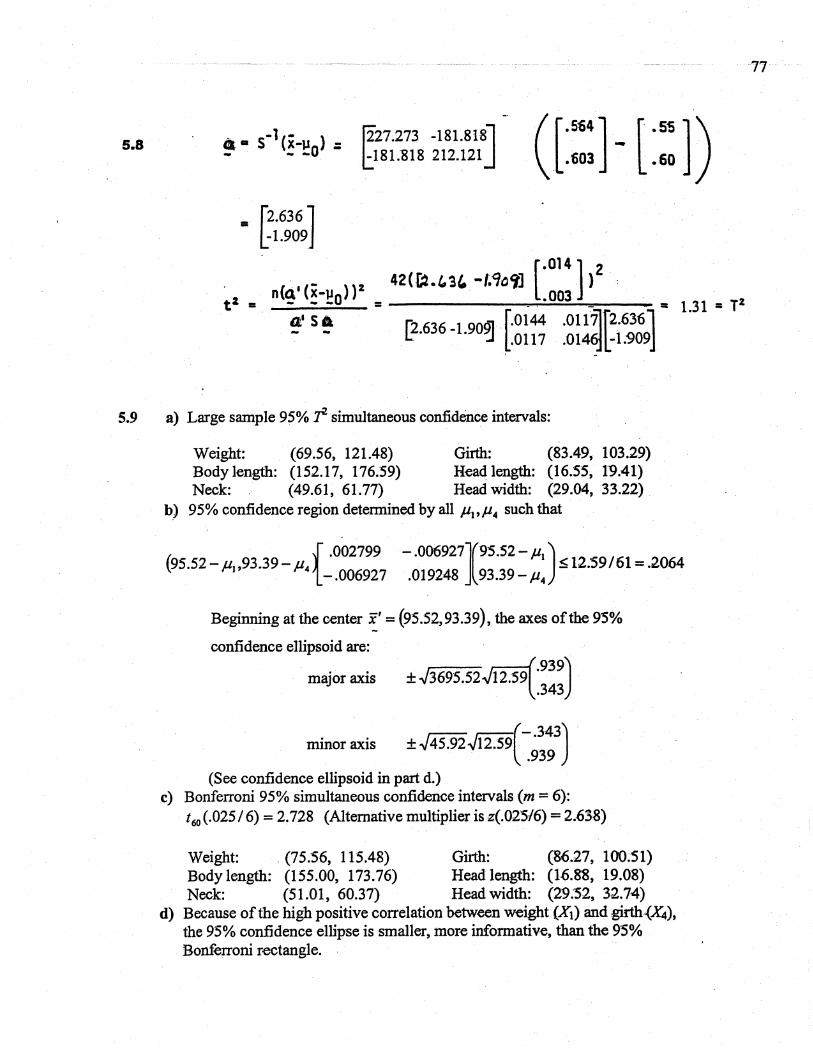
5.8-1(- )el CI S X-\1 .:- - -0 f227.273 -181.8181

t18L818 212.121 J((.Sti4 J -( .5'5 J )

.603 .60

= (2.636 J-1.909

tZ = n(~'(~-~O))Z =a' SA- -

(.014) 242(~.£,'3L. -1.9a'"J . )

.003

r2.636 -1 9091 .(.0144 .01 i71f2.63611. ':J .0117 .0146jL-i.909j

= 1.31 = TZ

5.9 a) Large sample 95% T simultaeous confdence intervals:

Weight: (69.56, 121.48) Girt: (83.49, 103.29)Body lengt: (152.17, 176.59) Head leng: (16.55, 19.41)

Neck: (49.61, 61.77) Head width: (29.04, 33.22)b) 95% confidence region determined by all Pi,P4 such that

L,002799 - .006927J(9S.52 -Pi)(95.52 - ,up93.39 -,u4 ~ 12.59/61 = .2064- .006927 .019248 93.39 - P4

Beginng at the center x' = (95.52,93.39), the axes of the 95%

confidence ellpsoid are:

major axis :t .J3695.52.Ji 2.5 9(' 939).343

:t .J45.92.J12.59(- .343).939

(See confidence ellpsoid in par d.)c) Bonferroni 95% simultaneous confidence intervals (m = 6):

160 (.025 / 6) = 2.728 (Alternative multiplier is z(.025/6) = 2.638)

. ,minor axis

Weight: . (75.56, 115.48) Gii1h: (86.27, 100.51)Body lengt: (155.00, 173.76) Head length: (16.~, 19.0g)Neck: (51.01, 60.37) Head width: (29.52, 32.74)

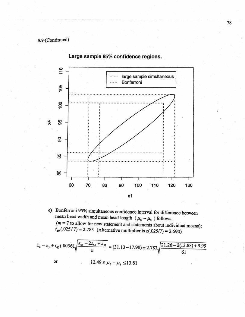
d) Because ofthe high positive correlation between weight (Xi) and girt~X4),the 95% confidence ellpse is smaller, more informative, than the 95%Bonferroni rectangle.

5.9 ,Continued)

0....

LO0..

00..

"' LO)( C'

0C'

LOCD

0CD

78

Large sample 95% confidence regions.

large sample simultaneousBonferroni

-- --- -~ -------- - - - - ---- - ----

- - - - - - - - - - - - - - - - -.

II .. . . . .. .. . . . . .'. .. . . . .. . ... . . . . . . . . . -' . . . . . . . . . . . . "l . . . . . . ~I I :: i :, : :i ,60 70 80 100 110 120 13090

x1

e) Bonferroni 95% simultaneous confidence interval for difference betweenmean head width and mean head lengt (,u6 - tls ) follows.

(m = 7 to allow for new statement and statements about individual means):t60 (.025/7) = 2.783 (Alternative multiplier is z(.025/7) = 2.690)

- (0036) S66 - 2sS6 + sss = (31.13 -17.98) +_ 2.78~~2i.26 -2(13.88) + 9.95x6 -xs :tt60 . Jn 61or 12.49:: tl6 -,us:: 13.81

79

5.10 a) 95% T simultanous confidence intervals:

Lngt: (13D.65, 155.93) Lngt4: (160.33, 185.95)

Lngt3: (127.00, 191.58) Lngt5: (155.37, 198.91)

b) 95% T- simultaneous intervals for change in lengt (ALngt):

~Lngth2-3: (-21.24, 53.24)~Lngt-4: (-22.70, 50.42)~Lngth4-5: (-20.69, 28.69)

c) 95% confidenceregon determined by all tl2-3,tl4-S such that

. ( i.Oll024 .009386J(16 - ,u2-3)16-tl2_3,4-tl4_s . ~72.96/7=10.42.009386 .025135 4 - ,u4-S

where ,u2-3 is the mean increase in length from year 2 to 3, and tl4-S isthe mean increase in length from year 4 to 5.

Beginnng at the center x' = (16,4), the axes of the 95% confidence

ellpsoid are:

maior axis.~~.895)

:tv157.8 72.96.- .447

( 447):t .J33.53.J72.96 .

.895

(See confidence ellpsoid in par e.)

mior axis

d) Bonferroni 95% simultaneous confdence intervals (m = 7):

Lngt: (137.37, 149.21)

Lngth3: (144.18, 174.40)

..6Lngth2-3: (-1.43, 33.43)

i1Lngt3-4: (-3.25, 30.97)

Lngt4: (167.14, 179.14)Lngth5: (166.95, 187.33)

i1Lngth4-5: (-7.55, 15.55)

-5.10 (Continued)

'80

e) The Bonferroni 95% confidence rectangle is much smaller and moreinformative than the 95% confidence ellpse.

0C\

0., ,.Iv::

0

0,.I

0C\

I

95% confidence regions.

o"l

oC" ...... .......... ....................................................

simultaneous T"2Bonferroni

III

I

IIII

II. I--~--------- ----------------~; I I: I I: I I; I I; I I; I I

.. . , . .~. . ... .. , ... , , . , . . . J. . . . . .. . .. , . . . , , . . . . , . . , , , . , .. . . .: i: I: I-20 o 20

J.2-3

40

81

5.11 a) E' =- (5.1856, 16.0700)

S = (176.0042 . 287.2412J;287.2412 527.8493

-1 ( .0508S =-.0276

~ .0276 J

.0169

Eigenvalues and eigenvectors of S:

,t = 688.759A

.42 = 15.094

,

£1 = (.49,.87),

i. = (.87,-.49)

§i 16Fp,n_p(.10) =: 7 F2.7(.10) = T (3.26) = 7.45~--Confidence Region

45

40

~L.

V)'ON)(

15 I 20 25 30 35 40 45

x1 ( C r )

35

-10 -,! '

I -10 J

b) 90% T intervals for the full data set:

Cr: (-6.88, 17.25) Sr: (-4.83, 36.97)

(.30, 1 OJ' is a plausible value for i..r-

82

5.11 (Continued)

c) Q-Q pJotsfor the margial distributions of

both varables

oi .

30

020

10

.o. ......-l. -UL .0.5 0.0 os 1.0 1.5

nomscor

Since r = 0.627 we rejec the hypothesis of normty for ths varable at a = 0.01

80

7I

eo

50

u; 40

30

20

10

0 .-1.

.

. .. ... .

-1.0 .0.5 0.0 0.5 1.0 1.5

nomsrSr

Since r= 0.818 we rejec the hypothesis of normty for this varable at a = 0.01

d) With data point (40.53, 73.68) removed,

ii = (.7675, 8.8688); r .3786S =b .03031.0303 J

69.8598.

-1 (2.7518S ·- .0406

-.0406 J

. 0149

1. F (.10)= 7(62t F" 6(.10) '" 164 (3.4'6) ~. 8.07-T p1n-p 'I90% r intervals: Cr: (.15, 1.9) Sc: (.47, 17.27)

83

5.12 Initial estimates are

( 4 i - - (0.5 0.0 0.5 i

'ß - 6, ~ - 2.0 0.0 .2 1.5The first revised estimates are

( 4.0833 i -( 0.6042 0.1667 0.8125 i

'ß = 6.0000 , E = 2.500 0.0.2.2500 1.9375

5.13 The X2distribution with 3 degrees of freeom.

5.14 Length of one-at-a time t-interval / Length of Bonferroni interval = tn_i(a/2)/tn_i(a/2m).

n 215 0.8546

25 0.8632

-50 0.8691

100 0.8718

00 0.8745

m4

0.74890.7644D.77490.7799"0.7847

10

0.64490.66780.68360.69110.6983

5.15

(0).

E(Xij) = (l)Pi + (0)(1 - Pi) = Pi.Var(Xij) = (1 - pi)2pi +(0 - p¡)2(1 - Pi) = Pi(1 - Pi)

(b). COV(Xij, Xkj) = E(XijXik) - E(Xij)E(Xkj) = 0 - PiPIi =-PiPk.

5.16

(6). Using Pj:: vx3.(0.05)VPj(1 - pj)ln, the 95 % confidence intervals for Pi, P2, 11, P4, Psare(0.221, 0.370),(0.258, 0.412), (0.098, 0.217), (0.029, 0.112),\0.084, .a.198) respectively.(b). Using Pi - ßi :l Vx3.(0.05)V(pi(1 - ßi) + ßi(1 - ßi) - 2ßiPi) In, the 95 % confdenceinterval for Pi - P2 is (-0.118, 0.0394), There is no significant difference in two proportions.

5.17

ßi = 0.585, ßi = 0.310, P3 = 0.105. Using Pj:l vx'5(O.-D5)VPj(1 - Pi)fn, the 95 %.confidence

intervals for Pi, P2, 11 are "(0.488, 0.682), (0.219, 0.401), ('0.044, 0.lô6), respectively.

84

5.18

\lo). Hotellng's T2 = 223.31. The critical point for the statistic (0: = 0.05) is 8.33. We rejectHo : fl = (500,50,30)'. That is, The group of students represented by scores are significantlydifferent from average college students.

(b). The lengths of three axes are 23.730,2.473, 1.183. And directions of corresponding ax..are

( 0.994 )

0.103 .,0.038

.(c). Data look fairly normaL.

( -0.104 )

0.995 ,0.006 ( -0.037 )

-0.010 .0.999

. . 35700 70 ~ -

. ..I- I"

-30 .

I' 60 r .60 I'

-i .I ~

.Lf M-

;C50 J x 25 -/ .

500i -.

40J -

..."1i 20 .i

o.--

400-

3015

-2 -1 0 1 2 -2 -1 0 1 2 .2 -1 0 1 2

NORMA SCORE NORMA SCORE NORMAL SCORE

700

600

. I... . ....

..- .'1...e : .._-, ..

. ..~..... .a. .I . ...0. . . ...- . , .

;c50' .

400

30 40 50 60 70

X2

700

.. .

70 0 . . .0I . . ..

. . 01 10

. . .60 :. .. 0

0 . ....! I.oi ..

N . 0 050 . o.x . .- .. ..40 i . .

. ..

30

15 20 2S 30 35

X3

60

... .a.. ..t : .. . ... . . .. . .. . . .. .. . .... i .: I... .. . .-... . ... .. .-.: :.o ..

x500

400.

o

15 20 2S 30 35

X3

5.19 a) The summary statistics are:

-x __ (18£0. 50Jn = 30,~354 .13

and s = (124055.17361621 .03

361"621 .031

348"6330.9'0 J

85

wher~ S has e i g~nva 1 ues and e; g~nv ect~rs

Å1 = 3407292

Å2 = 82748

e~ = (.105740, .994394)_1

!2 = (.994394,-.1 0574~)

Then, since 1 p(;:~) .Fp n_p(a) = 3~ 2~i) F2 2St .tl5) = .2306,, n, 'a 95% confidence region for ~- is given by the set of \1. -

(124055.17 3'61~21.03J' ~1(1860.5tl-~lJ(1860.'50-\11' 8354.13-~2) . .

361621 .03 348633tl. 90 83~4 .13-~2

. ~ .2306

The half lengths of the axes of this ellipse are 1.2300 Ir = 886.4 and

l. 2306 .~ = 138 ~ 1. Th~refore the ell ipse has the form-------_. --_...__.. . ...... --_..- .._._.. ".-----------_.- ------_._-

-~Ì"

'12,000 , :

-,

; /,. 10000 ; ,

, :j f

, '.:

, i

: ,.; I

; ;i

,

!,

; i /' . "Ji-- 'v..i ¡

,, ,

:, : , ¡ ,

,!

; , ; : ! ; ~ I: i :: ,~~.So . I

,

I i : ! !! :-

, '- , - -ß~5'4.13

i. i

:- : i

I;

! I,

l.1 :

; . I , i I l~ ... J I: : : ; i

,

; , ,11

: :,

, i : ! !

. i J i I, ,

ii .1

: ;. 1

::

';fJ"w: ;

, ,,

i : : :i

~E.

:¿--

,

I i , I1 , '. . IOQ" 2,.aoø. ' . 3öOO ' '. l.øo.ft Xl

86

b) Since ~O = (2000, 10000)' does not fall within the 9Siconfidence

ellipse, we would reJect the hypothesis HO:~ = ~O at the 5% level.

Thus, the data analyz~d are not consistent with these values.

c) The Q-Q plots for both stiffness and bending strength (see below)

show that the marginal normal ity is not seri ously viol ated. Ai so;

the correlation coefficients for the test of normal ity are .989 and

.990 respectively so that we fail to reject even at the ii signifi-

cance level. Finally, the scatter diagram (see below) does not indi-

cate departure from bivariate normality. So, the bivariate normal

distribution is a plausible probability model for these data.

Q-Q Plot-Bend i n9 StrengthX2

12000. . *

I.

!

* * *

10000.**

*****. ._-*

...._--------- -.- --

8000 .**

..2--..' ..*****

*- _.. .,-------***" ._-"- . -._--_._--

* * *

..._--- -_._-

6000. - ...... * ._--.._.._....... _. ------_.._---

4000. :i,

-2.0l

0.0 2.0-1.'0 1.~ 3.0

t:rr.e 1 at; on .989

Xi2800.

2400 .

::ooo.

1600 . ***** *

*

1200. **

800. .._----------- ._-- ..---"..

-2.0_ ____, ._-_ _=J.!.9..._

. _.._ . ..Correlation .. -.990 .

Q-Q Plot-Stiffness

* ****

*..

***2*2

****

* *

*

87

."__0"" ._____. .._--_ -_._---"

I

0.0.....-._.. ---~------I--:.

2.0_......-_.. ._.__....__.- ~.-

,.

1.0 ._ _ _ _.._~ .9.___

2400 ;. .

2000.

1600.

1200. . *

800.I

4000 .

Sea tter 01 agram

** .

*

* ** *

* ** * *** *. '.._-.- . ........_... .. . ...

*

*

***

*

***

'88

-_.. . -...._....~.. ..-

- -------- - ...-* .

--- ----_..-

*

**.....-_.._-- -_..__...

*

-- ---.- -._----

..._-_..__....- _.. ......._. .. ,...__. ---------

I

80ÖO.. - - 10000._._-~- .. .-:-6000.._-.. -- ---- . _._........--

.__.,.. .1---0- -~r.12000. X2.. . i 4000 .

89

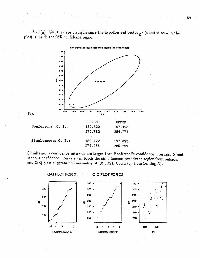
5.20 (6). Yes, they are plausible since the hypothesized vector eo (denoted as . in theplot) is inside the "95% confidence region. .

96li S1mullJeouB Cooldence Region for Wean Veclor

(11).

i i I

ii.ii.i .~

ii i

ii."¥ i.o

i ..i"

i' .

i, i

Uii' . ... 110 II .

Bonferroni C. i.:

Simultaneous C. i.:

'ii ,., ... 1'. ,.. "7 ...iiu.

LOWER UPPER189 .822 197 . 423274.782 284.774

189.422 197 .823274. 25S 285.299

Simultaneous confidence intervals are larger than Bonferroni's confidence intervals. Simul-taneous confidence intervals wil touch the simultaneous confidence region from outside.(c). Q~Q plots suggests non-normality of (Xii X2). Could try tra.nsforming XI.

Q-Q PLOT FOR X1

210 - .--..

200....

)(...

190---

.180 . ..

.2 -1 0 2

NORMAL SCORE

Q-Q PLOT FOR X2

310

. ..300 .

..290

.Jr

N 280x ./270 ..

260 .-..

250

-2 -1 0 2

NOMA SC-QRE

310. ..

300

29 . .. : - . ..280

..N .. . .x

270 . '.

260

250

ISO 20X1

90

5.21

HOTELLING T SQUARE - 9 .~218P-VALUE 0.3616

T2 INTERVAL BONFERRONIN MEAN STDEV TO TOxl 2S 0.84380 0.11402 .742 .946 .778 .909x2 25 0.81832 0.10685 .723 .914 .757 .880x3 25 1.79268 0.28347 1.540 2.046 1. 629 1. 95"6x4 25 1.73484 0.26360 1. 499 1. 970 1. 583 1. 887x5 25 0.70440 0.10756 .608 .800 .642 .766x6 25 0.69384 0.10295 .602 .786 .635 .753

The Bonferroni intervals use t ( .00417 ) - 2.88 and

the T2 intevals use the constant 4.465.

5.22

la). After eliminating outliers, the approximation to normality is improved.

91

a-a PLOT FOR X1 a-a PL-DT FOR X2 a-a PLOT FOR X3

30 18

2S 15 111

..'. 14 ..20 .

.. 12 .,.~ 10 ..X .. x 10 ,.'--15 .' ...C/ ,. - 8 ....10 _.. 5 -

6 0a: . . .' .W 5 . .. 4.

.. -2 -I 0 2 -2 .1 0 2 -2 -1 0 2l-:: NOMA SCRE NOMA SCORE NORMA SCORE0::l-~ 18 18

15 18 16. 14 . . 14.

12'. 12 ø. .~ 10 .. . . M

10 I. .X 10 , .. x ..l o .. .' 8 . o . 8 ...

5 ..8 6.. ..4 4

5 10 is 20 25 30 5 10 15 20 25 30 S 10 1S

Xi X1 X2

a-a PLOT FOR X1 a-a PLOT FOR X2 a-a PLOT FOR X3

14 . . 1818

16

CJ 14 . . 1214 .... ..

o. 10a: 12 ..12 ...

X..

~ 8 . '" ..W 10 ..- .. x 10 .""- 6 _.. .... 8. - 8 .... . 4 .l- . 66 . ..:: . 2 4 .4a -2 -1 0 2 .2 .1 0 2 -2 -I 0 2

l- NORMA SCRE NOM4 SCORE NOMA SCRE::a::l-~ iI ,.14

111 ILL1214. . 1410

12 .. . 12~ 8 . '"

:. .'" I... X 10 . . x 10 . .

. .II . . .

8 . ... . .4 . 6 II2

. . .4 4

4 II 8 10 14 4 8 8 10 14 2 4 6 8 10 14

XI X1 X2

l. Outliers remov.edi~

Bonferroni c. i.:

Simul taneous C. i.:

92

LOWER UPPER9.63 12.875.24 9.678.82 12.34

9.25 13.244.72 10.198.41 12.76

Simultaneous confidence intervals are larger than ßonferroni's confidence intervals.

(b) Full data set:

Bonferroni C. I.:

Simultaneous C. I.:

Lower9.795.788.65

Upper15.3310.5512.44

9.165.238.21

15.9611.0912.87

93

5.23 a) The data appear to be multivanate normal as shown by the "straightness" ofthe Q-Q plòts and chi-square plot below.

..140 -

.. 140 .. .. .. .- ..c . or .'t . 0) .CD 130 - . :i .x . Ul .t'lU 130 .:2 .

ID ......

120 - ..120

-1 i . I i

-2 -1 0 1 2 -2 -1 0 2NScMB NScBHi- = .97'6

~= .994

... . . .55 - .

110 - ... .. -s: . .c .- . C)C) . :i 50 - .-i . UlUl 100 - .lU .lU . Zm

.....

...45 -90 - ..

-T .1 I I , '. I ! i-2 -1 0 1 2 -2 -1 0 2NScBL NScNHr;= .995i. = .992

.10 - ..

.. .

d¿) .5 _. . .

.........

........

o - . ...I i

¡"U 5 10

.fe,4l.( -.5)/30)

5.23 (Continued)

94

b) Bonferroni 95% simultaneous confidence intervals (m = p = 4):t29 (.05/8) = 2.663

MaxBrt:BasHgth:BasLngth:NasHgt:

(128.87, 133.87)

(131.42, 135.78)

(96.32, 102.02)

(49.17, 51.89)

95% T simultaneous confidence intervals:

4(29) F (.05) = 3.49626 4.26

MaxBrt:BasHgt:BasLngt:NasHgth:

(128.08, 134.66)

(130.73, 136.47)

(95.43, 102.91)

(48.75, 52.31)

The Bonferroni intervals are slightly shorter than the T intervals.

9S

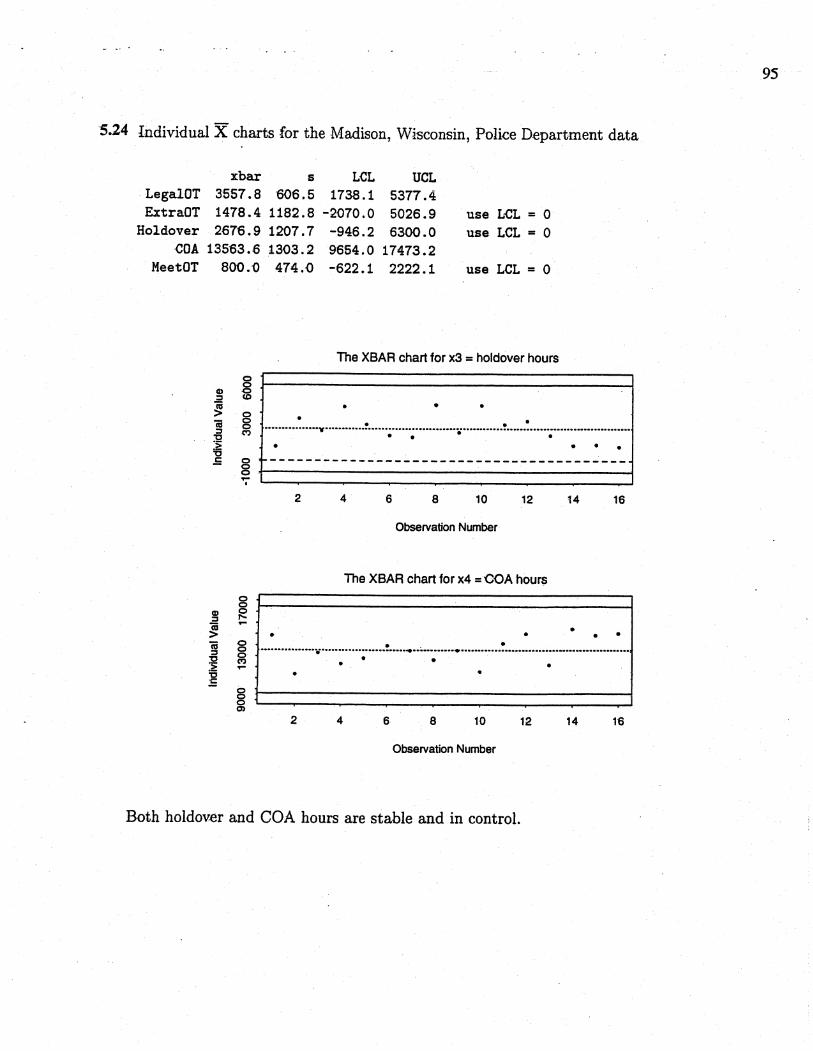
5.24 Individual X charts for the Madison, Wisconsin, Police Department data

xbar s LeL UCLLegalOT 3557.8 ô06.5 1738. 1 5377.4ExtraOT 1478.4 1182.8 -2.070.0 5026.9 use L-CL = 0

Holdover 2676.9 1207.7 -946 . 2 6300 . 0 use LCL = 0COA 13563.6 1303.2 9654.0 17473.2

MeetOT 800.0 474.0 -622. 1 2222 . 1 use LCL=O

00ai .0:: CD

ii;: 0ii 00:: (""C":;

'e.5 0.00..

.

00ai 0:: ,.ii ..;:ii .00:: a"C ("":; ..'e.5 000

Q)

The XBAR chart for x3 = holdover hours

. . .. .. ....a................y........................;..........;..........................__......................;................................

. . . .- - - - - - - - - - - - - - - - - - - - - - - - - - - - - - - - - - - - - - - -

2 4 6 8 10 12 14 16

Observation Number

The XBAR chart for x4 = COA hours

. .. . .. .............................................................--;........................................................................................

. .. .. .

2 4 6 8 10 1412 16

Observation Number

Both holdover and COA hours are stable and in control.

96

5.25 Quality ellpse and T2 chart for the holdover and COA overtime hours.

All points ar.e in control. The quality control 95% ellpse is

1.37x 10-6(X3 - 2677)2 + 1.18 x 10-6(X4 - 13564)2+1.80 X 1O-6(x3 - 2677)(X4 - 13564) =5.99.

The quality control 95% ellipse for

holdover hours and COA hours000r-..

000co..

.00 .0It ....

0 .in 0:i 0 .'I0 ..J: . .+c( .0 0u 00t' ... .

0 .00C\..

000T-T-

-1000 0 1000 3000 5000

Holdover Hours

a:r-

The 95% Tsq chart for holdover hours and COA hours

UCL = 5.991ci .................. '''..n..... ............ ........ ..... ...... .._...... ..... ..............._.._...........__.in

i:t! 'It'C\

o

97

5.26 T2 chart using the data on Xl = legal appearances overtime hours, X2 - extraordinary

event overtime hours, and X3 = holdover overtime hours. All points are in control.

The 99% Tsq chart based on x1, x2 and x3

o..................................................................................................................................................

.

CD

C'

~ co

vN

o

5.27 The 95% prediction ellpse for X3 = holdover hours and X4 = COA hours is

1.37x 10-6(x3 - 2677)2 + 1.18 x 1O-6(x4 - 13564)2

+1.80x 1O-6(x3 - 2677)(X4 - 13564) = 8.51.

The 95% control ellpse for future holdover hours

and COA hours

oooo..

000co.. .

...!!

0 .0j 0 .0 v:z .. . .+c( .0()

000N..

-1000 0 1000 3000 5000

Holdover Hours

98

5.28 (a)

x=

-.506-.207"-.062-.032

.698

-.065

s=

.0626 .0616

.0616 .0924

.0474 .0268

.0083 -.0008

.0197 .0228

.0031 .0155

.0474 .0083 .0197 .0031

.0268 -.0008 .0228 .0155

.1446 .0078 .0211 -.0049

.0078 .1086 .0221 .0066

.0211 .0221 .3428 .0146

-.0049 .0066 .0146 .0366

The fl char follows.

(b) Multivariate observations 20, 33,36,39 and 40 exceed the upper control limit.

The individual variables that contribute significantly to the out of control datapoints are indicated in the table below.

Point Variable P-ValueGrea ter Than UCL 20 Xl O. 0000

X2 0.00.01X3 0.0000X4 0.0105X5 0.0210X6 0.0032

33 X4 .0.0088X6 O. 0000

36 Xl o . 0000X2 \) .0000X3 \). OO.QO

X4 0.034339 X2 0.0198

X4 0.0001X5 0.0054X6 o . 000'0

40 XL 0.0000X2 O. 0088X3 0.0114X4 0.0-013

99

2 472' 2 29(6) .5.29 T = 12. . Since T = 12.472 c: -- F6,24 (.05) = 7.25(2.51) = 18.2 , we do not

reject H 0 : ¡. = 0 at the 5% leveL.

5.30 (a) Large sample 95% Bonferroni intervals for the indicated means follow.Multiplier is t49 (.05/2(6)):: z(.0042) = 2.635

Petroleum: .766:t 2.635(.9251,J) = .766:t .345 -7 (.421, 1.111)

Natural Gas: .508:t 2.635(.753/.J) = .508:t .282 -7 (.226, .790)

Coal: .438:t2.635(.4141.J) = .438:t.155 -7 (.283, .593)

Nuclear: .161:t 2.635(.207/.J) = .161 :t.076 -7 (.085, .237)

Total: 1.873:t 2.635(1.978/.J) = 1.873 :t.738 -7 (1.135, 2.611)

Petroleum - Natural Gas: .258:t2.635(.392/.J) = .258:t.146 -- (.112, .404)

(b) Large sample 95% simultaneous r intervals for the indicated means follow.

Multiplier is ~%;(.05) = .J9.49 = 3.081

Petroleum: .766:t3.081(.9251.J) = .766:t.404 -- (.362, 1.170)

Natural Gas: .508:t3.081(.753/.J) = .508:t.330 -- (.178, .838)

Coal: .438:t3.081(.414/.J) = .438:t.182 -- (.256, .620)

Nuclear: .161:t3.081(.207/.J) =.161:t.089 -- (.072, .250)

Total: 1.873:t 3.081(1.978/.J) = 1.873:t .863 -- (1.010, 2.736)

Petroleum - Natural Gas: .258:t 3.081(.392/.J) = .258:t .171-- (.087, .429)

Since the multiplier, 3.081, for the 95% simultaneous r intervals is larger thanthe multiplier, 2.635, for the Bonferroni intervals and everything else for a giveninterval is the same, the r intervals wil be wider than the Bonferroni intervals.

100

5.31 (a) The power transformation ~ = 0 (i.e. logarthm) makes the duration

observations more nearly normaL. The power transformation t = -0.5

(i.e. reciprocal of square root) makes the man/machine time observationsmore nearly normaL. (See Exercise 4.41.) For the transformed observations,

say Yi = In Xi' Y2 = 1/'¡ where Xl is duration and X2 is man/machine time,

- = p.171JY l .240 s = r .1513 -.0058J

l- .0058 .0018S-i - r 7.524 23.905J

l23.905 624.527

The eigenvalues for S are Â. = .15153, Â. = .00160 with corresponding, ,eigenvectors ei = (.99925 - .03866), e2 = (.03866 .99925l Beginning atcenter y, the axes of the 95% confidence ellpsoid are

maior axis: IT 2(24):! v Â. F2 23 (.05) ei = :t.208el25(23) .

. .mInor axis: r: 2(24):tvÂ. F223(.OS)e2 =:t.021e2

25(23) .

The ratio of the lengths of the major and minor axes, .416/.042 = 9.9, indicatesthe confidence ellpse is elongated in the ei direction.

(b) t24 (.05/2(2)) = 2.391, so the 95% confidence intervals for the two componentmeans (of the transformed observations) are:

Yi :tt24(.0125)¡; = 2.171:t2.391.J.1513 = 2.171:t.930 ~ (1.241, 3.101)

Y2 :tt24 (.0125)'¡ =.240:t2.391.J.0018 =.240:t.101 ~ (.139, .341)